Neural Video Depth Stabilizer

Abstract

Video depth estimation aims to infer temporally consistent depth. Some methods achieve temporal consistency by finetuning a single-image depth model during test time using geometry and re-projection constraints, which is inefficient and not robust. An alternative approach is to learn how to enforce temporal consistency from data, but this requires well-designed models and sufficient video depth data. To address these challenges, we propose a plug-and-play framework called Neural Video Depth Stabilizer (NVDS) that stabilizes inconsistent depth estimations and can be applied to different single-image depth models without extra effort. We also introduce a large-scale dataset, Video Depth in the Wild (VDW), which consists of 14,203 videos with over two million frames, making it the largest natural-scene video depth dataset to our knowledge. We evaluate our method on the VDW dataset as well as two public benchmarks and demonstrate significant improvements in consistency, accuracy, and efficiency compared to previous approaches. Our work serves as a solid baseline and provides a data foundation for learning-based video depth models. We will release our dataset and code for future research.

1 Introduction

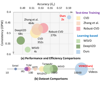
Figure 1: (a) Performance and efficiency comparisons. Circle area represents inference time. Smaller circles mean faster speed. The X-axis represents $\delta_{1}$ on Sintel [4] dataset for spatial accuracy. The Y-axis represents consistent metric $OPW$. Lower $OPW$ means better temporal consistency. Our framework outperforms prior arts by large margins. (b) Dataset comparisons. Larger circles mean larger amounts of frames. We present VDW dataset, the largest video depth dataset in the wild with diverse scenes.

Monocular video depth estimation is a prerequisite for various video applications, e.g., bokeh rendering [25, 47, 24], 2D-to-3D video conversion [12], and novel view synthesis [16, 17]. An ideal video depth model should output depth results with both spatial accuracy and temporal consistency. Although the spatial accuracy has been greatly improved by recent advances in single-image depth models [27, 28, 39, 45, 15] and datasets [18, 42, 41], how to obtain temporal consistency, i.e., removing flickers in the predicted depth sequences, is still an open question. The prevailing video depth approaches [23, 13, 48] require test-time training (TTT). During inference, a single-image depth model is finetuned on the testing video with geometry constraints and pose estimation. These TTT-based methods have two main issues: limited robustness and heavy computation overhead. Due to the heavy reliance on camera poses, e.g., CVD [23] shows erroneous predictions and robust-CVD [13] produces obvious artifacts for many videos when camera poses [29, 13] are inaccurate. Moreover, test-time training is extremely time-consuming. CVD [23] takes $40$ minutes for $244$ frames on four NVIDIA Tesla M40 GPUs.

This motivates us to build a learning-based model that learns to enforce temporal consistency from video depth data. However, like all the deep-learning models, learning-based paradigm requires proper model design and sufficient training data. Previous learning-based methods [34, 40, 46, 5] show worse performance than the TTT-based ones. Video depth data is also limited in scale and diversity.

To address the two aforementioned challenges, we first propose a flexible learning-based framework termed Neural Video Depth Stabilizer (NVDS), which can be directly applied to different single-image depth models. NVDS contains a depth predictor and a stabilization network. The depth predictor can be any off-the-shelf single-image depth model. Different from the previous learning-based methods [5, 40, 46, 34] that function as stand-alone models, NVDS is a plug-and-play refiner for different depth predictors. Specifically, the stabilization network processes initial flickering disparity estimated by the depth predictor and outputs temporally consistent results. Therefore, our framework can benefit from the cutting-edge depth models without extra effort. As for the design of stabilization network, inspired by attention [35] in other video tasks [14, 22, 1, 33], we adopt a cross-attention module in our framework. Each frame can attend relevant information from adjacent frames for temporal consistency. We also design a bidirectional inference strategy to further improve the consistency. As shown in Fig. 1(a), our NVDS outperforms the previous approaches in terms of consistency, accuracy, and efficiency significantly.

Moreover, we collect a large-scale natural-scene video depth dataset, Video Depth in the Wild (VDW), to support the training of robust learning-based models. Current video depth datasets are mostly closed-domain [9, 32, 31, 7, 37]. A few in-the-wild datasets [4, 38, 36] are still limited in quantity, diversity, and quality, e.g., Sintel [4] only contains $23$ animated videos. In contrast, our VDW dataset contains $14@203$ stereo videos of over $200$ hours and $2.23M$ frames from four different data sources, including movies, animations, documentaries, and web videos. We adopt a rigorous data annotation pipeline to obtain high-quality disparity ground truth for these data. As shown in Fig. 1(b), to the best of our knowledge, VDW is the largest in-the-wild video depth dataset with diverse scenes.

We conduct evaluations on the VDW and two public benchmarks: Sintel [4] and NYUDV2 [31]. Our method achieves state-of-the-art in both the accuracy and the consistency. We also fit three different depth predictors [27, 28, 45] into our framework and evaluate them on NYUDV2 [31]. The results demonstrate the flexibility and effectiveness of our plug-and-play manner. Our main contributions can be summarized as follows:

• We propose a plug-and-play and bidirectional learning-based framework termed Neural Video Depth Stabilizer (NVDS), which can be directly adapted to different single-image depth predictors to remove flickers.

• We propose VDW dataset, which is currently the largest video depth dataset in the wild with the most diverse video scenes.

2 Related Work

Consistent Video Depth Estimation. In addition to predicting spatial-accurate depth, the core task of consistent video depth estimation is to achieve temporal consistency, i.e., removing the flickering effects between consecutive frames. Current video depth estimation approaches can be categorized into test-time training (TTT) ones and learning-based ones. TTT-based methods train an off-the-shelf single-image depth estimation model on testing videos during inference with geometry [23, 13, 48] and pose [30, 29, 13] constraints. The test-time training can be time-consuming. For example, as illustrated by CVD [23], their method takes $40$ minutes on $4$ NVIDIA Tesla M40 GPUs to process a video of $244$ frames. Besides, TTT-based approaches are not robust on in-the-wild videos as they heavily rely on camera poses, which are not reliable for natural scenes. In contrast, the learning-based approaches train video depth models on video depth datasets by spatial and temporal supervision. ST-CLSTM [46] adopts long short-term memory (LSTM) to model temporal relations. FMNet [40] restores the depth of masked frames by the unmasked ones with convolutional self-attention [22]. Cao et al. adopt a spatial-temporal propagation network trained by knowledge distillation [10, 21]. However, those methods are independent and cannot refine the results from single-image depth models for consistency. Their performance on consistency and accuracy is also limited. For example, as shown by [40], ST-CLSTM [14] only exploits sub-sequences of several frames and produces obvious flickers in the outputs. In this paper, we propose a novel framework called Neural Video Depth Stabilizer (NVDS), which can be directly adapted to any off-the-shelf single-image depth models in a plug-and-play manner.

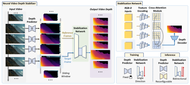
Figure 2: Overview of the neural video depth stabilizer. Our framework consists of a depth predictor and a stabilization network. The depth predictor can be any single-image depth model which produces initial flickering disparity maps. Then, the stabilization network refines the flickering disparity maps into temporally consistent ones. The stabilization network functions in a sliding window manner: the frame to be predicted fetches information from adjacent frames for stabilization. During inference, our NVDS framework can be directly adapted to any off-the-shelf depth predictors in a plug-and-play manner. We also devise bidirectional inference to further improve consistency.

Video Depth Datasets According to the scenes of samples, existing video depth datasets can be categorized into closed-domain datasets and natural-scene datasets. Closed-domain datasets only contain samples in certain scenes, e.g., indoor scenes [31, 7, 37], office scenes [32], and autonomous driving [9]. To enhance the diversity of samples, natural-scene datasets are proposed, which use computer-rendered videos [4, 38] or crawl stereoscopic videos from YouTube [36]. However, the scene diversity and scale of these datasets are still very limited for training robust video depth estimation models that can predict consistent depth in the wild. For instance, WSVD [36], which shares a few similar data annotation steps with the proposed VDW dataset, only contains $533$ YouTube videos with varied quality and insufficient diversity. Sintel [4] only contains $23$ animated videos. To better train and benchmark video depth models, we propose our VDW dataset with $14203$ videos from $4$ different data sources. To the best of our knowledge, our VDW dataset is currently the largest video depth dataset in the wild with the most diverse scenes.

3 Neural Video Depth Stabilizer

As shown in Fig. 2, the proposed Neural Video Depth Stabilizer (NVDS) consists of a depth predictor and a stabilization network. The depth predictor predicts the initial flickering disparity for each frame. The stabilization network converts the disparity maps into temporally consistent ones. Our NVDS framework can coordinate with any off-the-shelf single-image depth models as depth predictors. We also devise a bidirectional inference strategy to further enhance the temporal consistency during testing.

3.1 Stabilization Network

The stabilization network takes RGB frames along with initial disparity maps as inputs. A backbone [43] encodes the input sequences into depth-aware features. The next step is to build inter-frame correlations. We use a cross-attention module to refine the depth-aware features with temporal information from relevant frames. Finally, the refined features are fed into a decoder which restores disparity maps with temporal consistency.

Depth-aware Feature Encoding. Stabilization network works in a sliding-window manner: each frame refers to a few previous frames, which are denoted as reference frames, to stabilize the depth. We denote the frame to be predicted as the target frame. Each sliding window consists of four frames.

Due to the varied scale and shift of disparity maps produced by different depth predictors, the initial disparity maps within a sliding window $\mathbf{F}=\left\{F_{1},F_{2},F_{3},F_{4}\right\}$ should be normalized into $F_{i}^{norm}$:

$$F_{i}^{norm}=\frac{F_{i}-\min\left(\mathbf{F}\right)}{\max\left(\mathbf{F}\right)-\min\left(\mathbf{F}\right)}\,,i\in\left\{1,2,3,4\right\}.$$ (1)

Then, the normalized disparity maps are concatenated with the RGB frames to form a RGB-D sequence. We use a transformer backbone [43] to encode the RGB-D sequence into depth-aware feature maps.

Cross-attention Module. With the depth-aware features, the subsequent phase entails the establishment of inter-frame correlations. We leverage a cross-attention module to build temporal and spatial dependencies across pertinent video frames. Specifically, in the cross-attention module, the target frame selectively attends the relevant features in the reference frames to facilitate depth stabilization. Pixels in the target frame feature maps serve as the query in the cross-attention operation [35], while the keys and values are generated from the reference frames.

Computational cost can become prohibitively high when employing cross-attention for each position in depth-aware features. Hence, we utilize a patch merging strategy [8] to down-sample the target feature map. Besides, we also restrict the cross-attention into a local window, whereby each token in the target features can only attend a local window in the reference frames. Let $T$ denote the depth-aware feature of the target frame, while $R_{1},R_{2}$ and $R_{3}$ represent the features for the three reference frames. $T$ is partitioned into $7\times 7$ patches with no overlaps; each patch is merged into one token $\mathbf{t}\in\mathbb{R}^{c}$ , where $c$ is the dimension. For each $\mathbf{t}$, we conduct a local window pooling on $R_{1},R_{2},$ and $R_{3}$ and stack the pooling results into $R_{p}\in\mathbb{R}^{c\times 3}$. Then, the cross-attention is computed as:

$$\mathbf{t}^{\prime}=\mathrm{softmax}\frac{W_{q}\mathbf{t}\left(W_{k}R_{p}\right)^{T}}{\sqrt{c}}W_{v}R_{p}\,,$$ (2)

where $W_{q}$, $W_{k}$, and $W_{v}$ are learnable linear projections. The cross-attention layer is incorporated into a standard transformer block [35] with residual connection and multi-layer perceptron (MLP). We denote the resulting target feature map refined by the cross-attention module as $T_{tem}$.

Ultimately, a depth decoder with feature fusion modules [19, 20] integrates the depth-aware feature of the target frame ($T$) with the cross-attention refined feature $T_{tem}$, and predicts the consistent disparity map for target frame.

3.2 Training the Stabilization Network

In the training phase, only the stabilization network is optimized. The depth predictor is the freezed pre-trained DPT-L [27]. For the stabilization network, we apply spatial and temporal loss that supervises the depth accuracy and temporal consistency respectively. The training loss can be formulated by:

$$\mathcal{L}=\mathcal{L}_{s}(n-1)+\mathcal{L}_{s}(n)+\lambda\mathcal{L}_{t}(n,n-1)\,,$$ (3)

where $\mathcal{L}_{s}(n-1)$ and $\mathcal{L}_{s}(n)$ denote the spatial loss of frame $n-1$ and $n$ respectively. $\mathcal{L}_{t}(n,n-1)$ denotes the temporal loss between frame $n-1$ and $n$.

We adopt the widely-used affinity invariant loss and gradient matching loss [28, 27] as the spatial loss $\mathcal{L}_{s}$. As for the temporal loss, we adopt the optical flow based warping loss [5, 40] to supervise temporal consistency:

$$\begin{gathered}\mathcal{L}_{t}(n,n-1)=\frac{1}{M}\sum_{j=1}^{M}O^{(j)}_{n\Rightarrow n-1}||D^{(j)}_{n}-\hat{D}^{(j)}_{n-1}||_{1}\,,\end{gathered}$$ (4)

where $\hat{D}_{n-1}$ is the predicted disparity $D_{n-1}$ warped by the optical flow $FL_{n\Rightarrow n-1}$. In our implementation, we adopt the GMFlow [44] for optical flow. $O_{n\Rightarrow n-1}$ is the mask calculated as [5, 40] and $M$ denotes pixel numbers. See supplementary for more details on loss functions.

3.3 Bidirectional Inference

Expanding the temporal receptive range can be beneficial for consistency, e.g., adding more former or latter reference frames. However, directly training the stabilization network with bidirectional reference frames will introduce large training burdens. To remedy this, we only train the stabilization network with the former three reference frames. To further enlarge the temporal receptive field and enhance consistency, we introduce a bidirectional inference strategy.

Unlike the training phase, during inference, both the former and latter frames will be used as the reference frames. An additional sliding window is added, where the reference frames are the subsequent three frames of the target. Let us define the stabilizing process as a function $\mathcal{S}(V_{t},\mathbf{V}_{r})$, where $V_{t}$ and $\mathbf{V}_{r}$ denotes the target RGB-D frame and the reference frames set. When denoting the RGB-D sequence as $\{V_{j}|\,j\in{1,2,\cdots,N}\}$, $N$ represents frame numbers of a certain video, using this additional sliding window for stabilization can be formulated as:

$$D^{post}_{n}=\mathcal{S}(V_{n},\{V_{n+1},V_{n+2},V_{n+3}\})\,,$$ (5)

where $V_{n}$ denotes the target frame. Likewise, using the original sliding window for stabilization can be denoted by:

$$D^{pre}_{n}=\mathcal{S}(V_{n},\{V_{n-1},V_{n-2},V_{n-3}\})\,.$$ (6)

We ensemble the bidirectional results for a larger temporal receptive field as:

$$D^{bi}_{n}=\frac{(D^{pre}_{n}+D^{post}_{n})}{2}\,.$$ (7)

$D^{bi}_{n}$ denotes the final disparity prediction of the $n^{th}$ frame (target frame). This bidirectional manner can further improve the temporal consistency as demonstrated in Sec. 5.4.

Note that, the cross-attention module is shared by the two sliding windows for inference. Besides, the initial disparity maps and depth-aware features are pre-computed. Hence, the bidirectional inference only increases the inference time by $30\%$ compared with single-direction inference and brings no extra computation for the training process.

In addition to bidirectional inference, the depth predictor can be reconfigurable during inference. For example, simply using a more advanced model NeWCRFs [45] as the depth predictor can obtain performance gain without extra training, as shown in Table 5. As the depth accuracy can be inherited from state-of-the-art depth predictor, our neural video depth stabilizer (NVDS) framework can focus on the learning of depth stabilization and combine the depth accuracy with temporal consistency.

3.4 Implementation Details

Model Architecture. We use the DPT-L [27], Midas-v2 [28], and NeWCRFs [45] as the single-image depth predictors during inference, while only the disparity maps from DPT-L are used during training. Midas-v2 [28] is the same depth model as TTT-based methods [23, 13, 48] for fair comparisons. Mit-b5 [43] is adopted as the backbone to encode depth-aware features. For each target frame, we use three reference frames with inter-frame intervals $l=1$.

Training Recipe. All frames are resized so that the shorter side equals $384$, and then randomly cropped to $384\times 384$ for training. In each epoch, we randomly sample $72@000$ input sequences. Note that the sampled frames in each epoch does not overlap. We use Adam optimizer to train the model for $30$ epochs with a batchsize of $9$. The initial learning rate is set to $6e-5$ and decreases by $1e-5$ for every five epochs. When finetuning our model on NYUDV2 [31], we use a learning rate of $1e-5$ for only one epoch. In all experiments, the temporal loss weight $\lambda$ is set to $0.2$.

Type	Dataset	Videos	Frames($k$)	Indoor	Ourdoor	Dynamic	Resolution
Closed	NYUDV2 [31]	$464$	$407$	$\usym{2714}$	$\usym{2717}$	$\usym{2717}$	$640\times 480$
	KITTI [9]	$156$	$94$	$\usym{2717}$	$\usym{2714}$	$\usym{2714}$	$1224\times 370$
Domains	TUM [32]	$80$	$128$	$\usym{2714}$	$\usym{2717}$	$\usym{2714}$	$640\times 480$
	IRS [37]	$76$	$103$	$\usym{2714}$	$\usym{2717}$	$\usym{2717}$	$960\times 540$
	ScanNet [7]	$1@513$	$2@500$	$\usym{2714}$	$\usym{2717}$	$\usym{2717}$	$640\times 480$
Natural	Midas [28]	$\usym{2717}$	$75$	$\usym{2714}$	$\usym{2714}$	$\usym{2714}$	$1880\times 800$
	Sintel [4]	$23$	$1$	$\usym{2714}$	$\usym{2714}$	$\usym{2714}$	$1024\times 436$
Scenes	TartanAir [38]	$1@037$	$1@000$	$\usym{2714}$	$\usym{2714}$	$\usym{2717}$	$640\times 480$
	WSVD [36]	$553$	$1@500$	$\usym{2714}$	$\usym{2714}$	$\usym{2714}$	$\sim 720p$
	Ours	$14@203$	$2@237$	$\usym{2714}$	$\usym{2714}$	$\usym{2714}$	$1880\times 800$

Table 1: Comparisons of video depth datasets. The 3D Movies dataset of Midas [28] is not released and only contains 75k images but not videos. TartanAir [38] only has some limited dynamic scenes (e.g., fish in the ocean sequence). However, most videos in TartanAir [38] lack major dynamic objects (e.g., pedestrians). For example, models trained on TartanAir cannot predict satisfactory results in scenes with moving people as such scenes are rare. Our VDW dataset shows advantages in diversity and quantity.

4 VDW Dataset

As mentioned in Sec. 1, current video depth datasets are limited in both diversity and volume. To compensate for the data shortage and boost the performance of learning-based video depth models, we elaborate a large-scale natural-scene dataset, Video Depth in the Wild (VDW). To our best knowledge, our VDW dataset is currently the largest video depth dataset with the most diverse video scenes.

Dataset Construction. We collect stereo videos from four data sources: movies, animations, documentaries, and web videos. A total of $60$ movies, animations, and documentaries in Blu-ray format are collected. We also crawl $739$ web stereo videos from YouTube with the keywords such as “stereoscopic” and “stereo”. To balance the realism and diversity, only $24$ movies, animations, and documentaries are retained. For instance, “Seven Wonders of the Solar System” is removed as it contains many virtual scenes. The disparity ground truth is generated with two main steps: sky segmentation and optical flow estimation. A model ensemble manner is adopted to remove errors and noises in the sky masks, which can improve the quality of the ground truth and the performance of the trained models, especially on sky regions as shown in Fig. 5. A state-of-the-art optical flow model GMFlow [44] is used to generate the disparity ground truth. Finally, a rigorous data cleaning procedure is conducted to filter the videos that are not qualified for our dataset. Fig. 3 shows some examples of our VDW dataset.

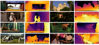
Figure 3: Examples of our VDW dataset. Four rows are from web videos, documentaries, animations, and movies, respectively. Sky regions and invalid pixels are masked out.

Figure 4: Objects presented in our VDW dataset. We conduct semantic segmentation with Mask2Former [6] trained on ADE20k [49]. Refer to our supplementary for more detailed construction process and data statistics.

Type	Method	Time($s$)	VDW			Sintel					NYUDV2
			$\delta_{1}\uparrow$	$Rel\downarrow$	$OPW\downarrow$		$\delta_{1}\uparrow$	$Rel\downarrow$	$OPW\downarrow$		$\delta_{1}\uparrow$	$Rel\downarrow$	$OPW\downarrow$
Single	Midas [28]	$0.76$	$0.651$	$0.288$	$0.676$		$0.485$	$0.410$	$0.843$		$0.910$	$0.095$	$0.862$
Image	DPT [27]	$0.97$	$\underline{0.730}$	$\underline{0.215}$	$0.470$		0.597	$\underline{0.339}$	$0.612$		$0.928$	$0.084$	$0.811$
Test-time	CVD [23]	$352.58$	$-$	$-$	$-$		$0.518$	$0.406$	$0.497$		$-$	$-$	$-$
Training	Robust-CVD [13]	$270.28$	$0.676$	$0.261$	$0.279$		$0.521$	$0.422$	$0.475$		$0.886$	$0.103$	$0.394$
	Zhang et al. [48]	$464.83$	$-$	$-$	$-$		$0.522$	$0.342$	$0.481$		$-$	$-$	$-$
Learning	ST-CLSTM [46]	$0.58$	$0.477$	$0.521$	$0.448$		$0.351$	$0.517$	$0.585$		$0.833$	$0.131$	$0.645$
Based	Cao et al. [5]	$-$	$-$	$-$	$-$		$-$	$-$	$-$		$0.835$	$0.131$	$-$
	FMNet [40]	$3.87$	$0.472$	$0.514$	$0.402$		$0.357$	$0.513$	$0.521$		$0.832$	$0.134$	$0.387$
	DeepV2D [34]	$68.71$	$0.546$	$0.528$	$0.427$		$0.486$	$0.526$	$0.534$		$0.924$	$0.082$	$0.402$
	WSVD [36]	$4.25$	$0.637$	$0.314$	$0.462$		$0.501$	$0.439$	$0.577$		$0.768$	$0.164$	$0.683$
	Ours(Midas)	$1.55$	$0.700$	$0.240$	$\underline{0.180}$		$0.532$	$0.374$	$\underline{0.469}$		$\underline{0.941}$	$\underline{0.076}$	$\underline{0.373}$
	Ours(DPT)	$1.73$	0.742	0.208	0.147		$\underline{0.591}$	0.335	0.424		0.950	0.072	0.364

Table 2: Comparisons with the state-of-the-art approaches. We report the total time of processing eight $640\times 480$ frames by different methods on one NVIDIA RTX A6000 GPU. Best performance is in boldface. Second best is underlined.

Dataset Statistics. VDW dataset contains $14@203$ videos with a total of $2@237@320$ frames. The total data collection and processing time takes over six months and about $4@000$ man-hours. To verify the diversity of scenes and entities in our dataset, we conduct semantic segmentation by Mask2Former [6] trained on ADE20k [49]. All the $150$ categories are covered in our dataset, and each category can be found in at least $50$ videos. Fig. 4 shows the word cloud of the 150 categories. We randomly choose $90$ videos with $12@622$ frames as the test set. The testing videos adopt different data sources from the training data, i.e., different movies, web videos, or animations. Our VDW not only alleviates the data shortage for learning-based approaches, but also serves as a comprehensive benchmark for video depth.

Comparisons with Other Datasets. As shown in Table 1, the proposed VDW dataset has significantly larger numbers of video scenes. Compared with the closed-domain datasets [31, 9, 7, 32, 37], the videos of VDW are not restricted to a certain scene, which is more helpful to train a robust video depth model. For the natural-scene datasets, our dataset has more than ten times the number of videos as the previous largest dataset WSVD [36]. Although WSVD [36] has $1.5M$ frames, the scenes (video numbers) are limited. Midas [28] also proposes their 3D Movies dataset with in-the-wild images and disparity. Compared with the 3D Movies dataset of Midas [28], VDW differs in two main aspects: (1) accessibility; and (2) dataset scale and format. Their 3D Movies dataset [28] is not released and only contains $75k$ images. In contrast, VDW contains 14,203 videos with $2.237M$ frames. It is also worth noticing that our VDW dataset has higher resolution and a rigorous data annotation and cleaning pipeline. We only collect videos with resolutions over $1080p$ and crop all our videos to $1880\times 800$ to remove black bars and subtitles. See supplementary for more statistics and construction process.

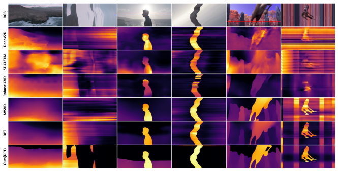
Figure 5: Qualitative comparisons. DeepV2D [34] and Robust-CVD [13] show obvious artifacts in those videos. We draw the scanline slice over time; fewer zigzagging pattern means better consistency. Compared with the other video depth methods, our NVDS is more robust on natural scenes and achieves better spatial accuracy and temporal consistency.

5 Experiments

To prove the effectiveness of our framework Neural Video Depth Stabilizer (NVDS), we conduct experiments on $3$ different datasets, which contain videos for real-world and synthetic, static and dynamic, indoor and outdoor.

5.1 Datasets and Evaluation Protocol

VDW Dataset. We use the proposed VDW as the training data for its diversity and quantity on natural scenes. We also evaluate the previous video depth approaches on the test split of VDW, serving as a new video depth benchmark.

Sintel Dataset. Following [13, 48], we use the final version of Sintel [4] to demonstrate the generalization ability of our NVDS. We conduct zero-shot evaluations on Sintel [4]. All learning-based methods are not finetuned on Sintel dataset.

NYUDV2 Dataset. Except for natural scenes, a closed-domain NYUDV2 [31] is adopted for evaluation. We pretrain the stabilization network on VDW and finetune the model on NYUDV2 [31] dataset. Besides, we also test our NVDS on DAVIS [26] for qualitative comparisons.

Evaluation Metrics. We evaluate both the depth accuracy and temporal consistency of different methods. For the temporal consistency metric, we adopt the optical flow based warping metric ($OPW$) following FMNet [40], which can be computed as:

$$OPW=\frac{1}{N-1}\sum_{n=2}^{N}\mathcal{L}^{t}(n,n-1)\,.$$ (8)

We report the average $OPW$ of all the videos in the testing sets. As for the depth metrics, we adopt the commonly-applied $Rel$ and $\delta_{i}(i=1,2,3)$.

Method	$\delta_{1}\uparrow$	$\delta_{2}\uparrow$	$\delta_{3}\uparrow$	$Rel\downarrow$	$OPW\downarrow$
SC-DepthV1 [3]	$0.813$	$0.952$	$0.987$	$0.143$	$0.465$
SC-DepthV2 [2]	$0.820$	$0.956$	$0.989$	$0.138$	$0.474$
ST-CLSTM [46]	$0.833$	$0.965$	$0.991$	$0.131$	$0.645$
Cao et al. [5]	$0.835$	$0.965$	$0.990$	$0.131$	$-$
FMNet [40]	$0.832$	$0.968$	$0.992$	$0.134$	$0.387$
DeepV2D [34]	$0.924$	$0.982$	$0.994$	$0.082$	$0.402$
Ours-scratch(DPT)	0.931	0.988	0.997	0.081	0.372

Table 3: Comparisons of the learning-based approaches on NYUDV2 [31] dataset. All the compared methods use NYUDV2 [31] as the training and evaluation data. Our neural video depth stabilizer trained from scratch also achieves better performance than all the other methods.

5.2 Comparisons with Other Video Depth Methods

Comparisons with the TTT-based methods. First focus on the test-time training (TTT) approaches [23, 13, 48]. As shown in Table 2, our learning-based framework outperforms TTT-based approaches by large margins in terms of inference speed, accuracy and consistency. Our NVDS shows at least $6.6\%$ and $7.6\%$ improvements for $\delta_{1}$ and $OPW$ than Robust-CVD [13] on VDW, Sintel [4], and NYUDV2 [31]. Our learning-based approach is over one hundred times faster than Robust-CVD [13]. Our strong performance demonstrates that learning-based frameworks are capable of attaining great performance with much higher efficiency than TTT-based methods [23, 13, 48].

It is also worth-noticing that the TTT-based approaches are not robust for natural scenes. CVD [23] and Zhang et al. [48] fail on some videos on VDW and Sintel [4] dataset due to erroneous pose estimation results. Hence, some of their results are not reported in Table 2. Refer to supplementary for more details. Although Robust-CVD [13] can produce results for all testing videos by jointly optimizing the camera poses and depth, it is still not robust for many videos and produces obvious artifacts as shown in Fig. 5.

Comparisons with the learning-based methods. The proposed neural video depth stabilizer also attains better accuracy and consistency than previous learning-based approaches [46, 40, 5, 36] on all the three datasets, including natural scenes and closed domain. As shown in Table 2, on our VDW and Sintel with natural scenes, the proposed NVDS shows obvious advantages: improving $\delta_{1}$ and $OPW$ by over $9\%$ and $18.6\%$ compared with previous learning-based methods. Note that, our NVDS can benefit from stronger single-image models and obtain better performance, which will be discussed in Table 5.

To better compare NVDS with previous learning-based method, we only use NYUDV2 [31] as training and evaluation data for comparisons. As shown in Table 3, the proposed NVDS improves the FMNet [40] by $9.9\%$ and $3.8\%$ in terms of $\delta_{1}$ and $OPW$ . We also achieve better performance than DeepV2D [34], which is the previous state-of-the-art structure-from-motion-based methods but can only deal with completely static scenes. The results demonstrate that using our architecture alone can also obtain better video depth performance.

Dataset	$\delta_{1}\uparrow$	$OPW\downarrow$
NYUDV2	$0.527$	$0.435$
IRS+TartanAir	$0.542$	$0.489$
VDW(Ours)	0.591	0.424

(a) Different Training Data

Setting	$\delta_{1}\uparrow$	$OPW\downarrow$
Scratch(DPT)	$0.931$	$0.372$
Pretrain(Midas)	$0.941$	$0.373$
Pretrain(DPT)	0.950	0.364

(b) Pretraining and Finetuning

Table 4: Influence of different training data. (a) Training with different datasets. We conduct zero-shot evaluations on Sintel [4] with different training data for our NVDS. (b) Pretraining and finetuning. Pretraining on our VDW can further improve the results on the closed-domain NYUDV2 [31], compared with training from scratch.

	Initial			Ours
	$\delta_{1}\uparrow$	$Rel\downarrow$	$OPW\downarrow$		$\delta_{1}\uparrow$	$Rel\downarrow$	$OPW\downarrow$
Midas [28]	$0.910$	$0.095$	$0.862$		$0.941$	$0.076$	$0.373$
DPT [27]	$0.928$	$0.084$	$0.811$		$0.950$	$0.072$	$0.364$
NeWCRFs [45]	0.937	0.072	0.645		0.957	0.068	0.326

Table 5: Comparisons of different depth predictors on the NYUDV2 [31] dataset. Our framework is compatible with different depth predictors in a plug-and-play manner.

Qualitative Comparisons. We show some qualitative comparisons on natural-scene videos in Fig. 5. We draw the scanline slice over time. Fewer zigzagging pattern means better consistency. The initial estimation of DPT [27] in the sixth row contains flickers and blurs, which are eliminated with the proposed NVDS, as shown in the last row. Although the TTT-based Robust-CVD [13] shows competitive performances on the indoor NYUDV2 [31] dataset, it is not robust on the natural scenes. As can be observed in the fourth row, Robust-CVD produces obvious artifacts due to erroneous pose estimation.

One can also observe that we produce much sharper estimation at the edges, especially on the skylines, which can be down to our rigorous annotation pipeline for VDW, e.g., the ensemble strategy for sky segmentation.

Influence of Training Data. The quality and diversity of data can greatly influence the learning-based video depth models. Our VDW dataset offers hundreds of times more data and scenes compared to previous works, which can be used to train robust learning-based models in the wild. To better show the difference, we compare our dataset with the existing datasets under zero-shot cross-dataset setting. As shown in Table 4 (a), we train our NVDS with existing video depth datasets [31, 37, 38] and evaluate the model on Sintel [4] dataset. With both quantity and diversity, using VDW as the training data yields the best accuracy and consistency. Our VDW dataset is far more diverse for training robust video depth models, compared with large closed-domain dataset NYUDV2 [31] or synthetic natural-scene dataset like IRS [37] and TartanAir [38].

Moreover, although the proposed VDW is designed for natural scenes, it can also boost the performance on closed domains by serving as pretraining data. As in Table 4 (b), the VDW-pretrained model outperforms the model that is trained from scratch, even with weaker single-image model (Midas [28]). This suggests that VDW can also benefit some closed-domain scenarios.

Method	$\delta_{1}\uparrow$	$OPW\downarrow$
DPT [27]	$0.730$	$0.470$
Pre-window	$0.741$	$0.165$
Post-window	$0.741$	$0.174$
Bidirectional	0.742	0.147

(a) DPT Initialization

Method	$\delta_{1}\uparrow$	$OPW\downarrow$
Midas [28]	$0.651$	$0.676$
Pre-window	$0.700$	$0.207$
Post-window	$0.699$	$0.218$
Bidirectional	0.700	0.180

(b) Midas Initialization

Table 6: Ablation of bidirectional inference on VDW. Bidirectional inference with larger temporal receptive fields can further improve the consistency.

	DPT-L [27]	NeWCRFs [45]	Midas-v2 [28]	Stabilization Network
FLOPs ($G$)	$1011.32$	$550.47$	$415.24$	$254.53$
Params ($M$)	$341.26$	$270.33$	$104.18$	$88.31$

Table 7: Comparisons of FlOPs and model parameters. We evaluate the efficiency of our stabilization network and different depth predictors [28, 27, 45]. The FlOPs are evaluated on a $384\times 384$ video with four frames.

5.3 Model Efficiency Comparisons

To evaluate the efficiency, we compare the inference time on a $640\times 480$ video with eight frames. The inference is conducted on one NVIDIA RTX A6000 GPU. As shown in Table 2, the proposed NVDS reduces the inference time by hundreds of times compared to the TTT-based approaches CVD [23], Robust-CVD [13], and Zhang et al. [48]. The learning-based method DeepV2D [34] alternately estimates depth and camera poses, which is time-consuming. WSVD [36] is also slow because they need to compute optical flow [11] between consecutive frames while inference.

We also evaluate the efficiency of the proposed stabilization network and different depth predictors. Model parameters and FLOPs are reported in Table 7. The FlOPs are evaluated on a $384\times 384$ video with four frames. Our stabilization network only introduces limited computation overhead compared with the depth predictors [28, 27, 45].

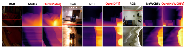
Figure 6: Visual results on NYUDV2 [31] dataset. We compare NVDS with three different depth predictors [28, 27, 45].

5.4 Ablation Studies

Here we verify the effectiveness of the proposed method. We first ablate the plug-and-play manner with different single-image depth models. Besides, We also discuss the bidirectional inference, the temporal loss, the reference frames, and baselines without the stabilization network.

Plug-and-play Manner. As shown in Table 5, we directly adapt our NVDS to three different state-of-the-art single-image depth models DPT [27], Midas [28], and NeWCRFs [45]. For NeWCRFs [45], we adopt their official checkpoint on NYUDV2 [31]. By post-processing their initial flickering disparity maps, our NVDS achieves better temporal consistency and spatial accuracy. With higher initial depth accuracy, the spatial performance of our NVDS is also improved. The experiment demonstrates the effectiveness of our plug-and-play manner. Visual comparisons with those three depth predictors are shown in Fig. 6. Depth maps and scanline slice prove our accuracy and consistency.

Method	$\delta_{1}\uparrow$	$OPW\downarrow$
DPT [27]	$0.621$	$0.492$
$w/o\;\mathcal{L}^{t}$	0.627	$0.303$
$w/\;\mathcal{L}^{t}$	$0.625$	0.216

(a) Temporal Loss

Method	$\delta_{1}\uparrow$	$OPW\downarrow$
$l=1$	0.625	0.216
$l=3$	$0.618$	$0.219$
$l=5$	$0.621$	$0.246$

(b) Inter-frame Intervals

Table 8: Temporal loss and inter-frame intervals l. We randomly split $100$ videos for training and $10$ videos for testing from our VDW dataset in these two experiments.

Bidirectional Inference. As shown in Table 6, whether using DPT [27] or Midas[28] as the single-image depth predictor, our NVDS can already enforce the temporal consistency with previous or post sliding window of target frame. The bidirectional inference can further improve the consistency with larger bidirectional temporal receptive fields.

Temporal Loss. As in Table 8 (a), without the temporal loss as explicit supervision, our stabilization network can enforce temporal consistency. Adding the temporal loss can further remove flickers and improve temporal consistency.

Reference Frame Intervals. We denote the inter-frame intervals as $l$. As shown in Table 8 (b), $l=1$ attains the best performance in our experiments.

Reference Frame Numbers. As shown in Table 9 (b), using three reference frames ($n$=3) for a target frame achieves the best results. More reference frames ($n$=4) increase computational costs but bring no improvement, which can be caused by the temporal redundancy of videos.

Baselines without Stabilization Network. With DPT as the depth predictor, we train and evaluate two baselines without the stabilization network on the same subset as Table 8. We use the same temporal window as NVDS. The first baseline (Single-frame) can only process each frame independently. Temporal window and loss $\mathcal{L}_{t}$ are used for consistency. The second baseline (Multi-frame) uses neighboring frames concatenated by channels to predict depth of the target frame. Training and inference strategies are kept the same as NVDS. As shown in the Table 9 (a), temporal flickers cannot be solved by simply adding temporal windows and training loss on those baselines. Proper designs are needed for inter-frame correlations. Our stabilization network improves consistency ($OPW$) significantly.

DPT w/	Single-frame	Multi-frame	Ours
$\delta_{1}\uparrow$	$0.615$	$0.608$	0.625
$OPW\downarrow$	$0.488$	$0.471$	0.216

(a) $W/o$ Stabilization Network

	n=1	n=2	n=3	n=4
$\delta_{1}\uparrow$	$0.618$	$0.622$	0.625	$0.625$
$OPW\downarrow$	$0.272$	$0.233$	0.216	$0.224$

(b) Reference Frame Numbers

Table 9: Baselines without NVDS stabilization network and reference frames numbers n. The experiment is conducted on the same VDW subset as Table 8.

6 Conclusion

In this paper, we propose a Neural Video Depth Stabilizer framework and a large-scale natural-scene VDW dataset for video depth estimation. Different from previous learning-based video depth models that function as stand-alone models, our Neural Video Depth Stabilizer learns to stabilize the flickering results from the estimations of single-image depth models. In this way, Neural Video Depth Stabilizer can focus on the learning of temporal consistency, while inheriting the depth accuracy from the cutting-edge depth predictors without further tuning. We also elaborate on the VDW dataset to alleviate the data shortage. To our best knowledge, it is currently the largest video depth dataset in the wild. We hope our work can serve as a solid baseline and provide a data foundation for the learning-based video depth models.

Limitations and future work. Currently, we only offer one implementation for the NVDS framework. In future work, we will consider using more mechanisms in the stabilization network and adding more implementations for different applications, e.g., the lightweight models.

Acknowledgments. This work was funded by Adobe Research. Meanwhile, our work is also supported under the RIE2020 Industry Alignment Fund - Industry Collaboration Projects (lAF-ICP) Funding Initiative, as well as cash and in-kind contribution from the industry partner(s).

References

- [1] Anurag Arnab, Mostafa Dehghani, Georg Heigold, Chen Sun, Mario Lučić, and Cordelia Schmid. Vivit: A video vision transformer. In Proceedings of the IEEE/CVF International Conference on Computer Vision (ICCV), pages 6836–6846, 2021.
- [2] Jia-Wang Bian, Huangying Zhan, Naiyan Wang, Tat-Jun Chin, Chunhua Shen, and Ian Reid. Auto-rectify network for unsupervised indoor depth estimation. IEEE transactions on pattern analysis and machine intelligence, 44(12):9802–9813, 2022.
- [3] Jia-Wang Bian, Huangying Zhan, Naiyan Wang, Zhichao Li, Le Zhang, Chunhua Shen, Ming-Ming Cheng, and Ian Reid. Unsupervised scale-consistent depth learning from video. International Journal of Computer Vision (IJCV), 2021.
- [4] Daniel J Butler, Jonas Wulff, Garrett B Stanley, and Michael J Black. A naturalistic open source movie for optical flow evaluation. In European Conference on Computer Vision (ECCV), pages 611–625. Springer, 2012.
- [5] Yuanzhouhan Cao, Yidong Li, Haokui Zhang, Chao Ren, and Yifan Liu. Learning structure affinity for video depth estimation. In Proceedings of the 29th ACM International Conference on Multimedia, pages 190–198, 2021.
- [6] Bowen Cheng, Ishan Misra, Alexander G Schwing, Alexander Kirillov, and Rohit Girdhar. Masked-attention mask transformer for universal image segmentation. In Proceedings of the IEEE/CVF Conference on Computer Vision and Pattern Recognition (CVPR), pages 1290–1299, 2022.
- [7] Angela Dai, Angel X Chang, Manolis Savva, Maciej Halber, Thomas Funkhouser, and Matthias Nießner. Scannet: Richly-annotated 3d reconstructions of indoor scenes. In Proceedings of the IEEE/CVF Conference on Computer Vision and Pattern Recognition (CVPR), pages 5828–5839, 2017.
- [8] Alexey Dosovitskiy, Lucas Beyer, Alexander Kolesnikov, Dirk Weissenborn, Xiaohua Zhai, Thomas Unterthiner, Mostafa Dehghani, Matthias Minderer, Georg Heigold, Sylvain Gelly, et al. An image is worth 16x16 words: Transformers for image recognition at scale. In International Conference on Learning Representations, 2020.
- [9] Andreas Geiger, Philip Lenz, Christoph Stiller, and Raquel Urtasun. Vision meets robotics: The kitti dataset. The International Journal of Robotics Research, 32(11):1231–1237, 2013.
- [10] Geoffrey Hinton, Oriol Vinyals, Jeff Dean, et al. Distilling the knowledge in a neural network. arXiv preprint arXiv:1503.02531, 2(7), 2015.
- [11] Eddy Ilg, Nikolaus Mayer, Tonmoy Saikia, Margret Keuper, Alexey Dosovitskiy, and Thomas Brox. Flownet 2.0: Evolution of optical flow estimation with deep networks. In Proceedings of the IEEE/CVF Conference on Computer Vision and Pattern Recognition (CVPR), pages 2462–2470, 2017.
- [12] Kevin Karsch, Ce Liu, and Sing Bing Kang. Depth transfer: Depth extraction from video using non-parametric sampling. IEEE transactions on pattern analysis and machine intelligence, 36(11):2144–2158, 2014.
- [13] Johannes Kopf, Xuejian Rong, and Jia-Bin Huang. Robust consistent video depth estimation. In Proceedings of the IEEE/CVF Conference on Computer Vision and Pattern Recognition (CVPR), pages 1611–1621, 2021.
- [14] Jiangtong Li, Wentao Wang, Junjie Chen, Li Niu, Jianlou Si, Chen Qian, and Liqing Zhang. Video semantic segmentation via sparse temporal transformer. In Proceedings of the 29th ACM International Conference on Multimedia, MM ’21, page 59–68, New York, NY, USA, 2021. Association for Computing Machinery.
- [15] Jiaqi Li, Yiran Wang, Zihao Huang, Jinghong Zheng, Ke Xian, Zhiguo Cao, and Jianming Zhang. Diffusion-augmented depth prediction with sparse annotations. arXiv preprint arXiv:2308.02283, 2023.
- [16] Xingyi Li, Zhiguo Cao, Huiqiang Sun, Jianming Zhang, Ke Xian, and Guosheng Lin. 3d cinemagraphy from a single image. In Proceedings of the IEEE/CVF Conference on Computer Vision and Pattern Recognition (CVPR), pages 4595–4605, June 2023.
- [17] Xingyi Li, Chaoyi Hong, Yiran Wang, Zhiguo Cao, Ke Xian, and Guosheng Lin. Symmnerf: Learning to explore symmetry prior for single-view view synthesis. In Proceedings of the Asian Conference on Computer Vision (ACCV), pages 1726–1742, December 2022.
- [18] Zhengqi Li and Noah Snavely. Megadepth: Learning single-view depth prediction from internet photos. In Proceedings of the IEEE/CVF Conference on Computer Vision and Pattern Recognition (CVPR), June 2018.
- [19] Guosheng Lin, Anton Milan, Chunhua Shen, and Ian Reid. Refinenet: Multi-path refinement networks for high-resolution semantic segmentation. In Proceedings of the IEEE/CVF Conference on Computer Vision and Pattern Recognition (CVPR), pages 1925–1934, 2017.
- [20] Tsung-Yi Lin, Piotr Dollár, Ross Girshick, Kaiming He, Bharath Hariharan, and Serge Belongie. Feature pyramid networks for object detection. In Proceedings of the IEEE/CVF Conference on Computer Vision and Pattern Recognition (CVPR), pages 2117–2125, 2017.
- [21] Yifan Liu, Ke Chen, Chris Liu, Zengchang Qin, Zhenbo Luo, and Jingdong Wang. Structured knowledge distillation for semantic segmentation. In Proceedings of the IEEE/CVF Conference on Computer Vision and Pattern Recognition (CVPR), pages 2604–2613, 2019.
- [22] Zhouyong Liu, Shun Luo, Wubin Li, Jingben Lu, Yufan Wu, Shilei Sun, Chunguo Li, and Luxi Yang. Convtransformer: A convolutional transformer network for video frame synthesis. arXiv preprint arXiv:2011.10185, 2020.
- [23] Xuan Luo, Jia-Bin Huang, Richard Szeliski, Kevin Matzen, and Johannes Kopf. Consistent video depth estimation. ACM Transactions on Graphics (ToG), 39(4):71–1, 2020.
- [24] Xianrui Luo, Juewen Peng, Ke Xian, Zijin Wu, and Zhiguo Cao. Defocus to focus: Photo-realistic bokeh rendering by fusing defocus and radiance priors. Information Fusion, 89:320–335, 2023.
- [25] Juewen Peng, Zhiguo Cao, Xianrui Luo, Hao Lu, Ke Xian, and Jianming Zhang. Bokehme: When neural rendering meets classical rendering. In Proceedings of the IEEE/CVF Conference on Computer Vision and Pattern Recognition (CVPR), pages 16283–16292, 2022.
- [26] Jordi Pont-Tuset, Federico Perazzi, Sergi Caelles, Pablo Arbeláez, Alexander Sorkine-Hornung, and Luc Van Gool. The 2017 davis challenge on video object segmentation. arXiv preprint arXiv:1704.00675, 2017.
- [27] René Ranftl, Alexey Bochkovskiy, and Vladlen Koltun. Vision transformers for dense prediction. In Proceedings of the IEEE/CVF International Conference on Computer Vision (ICCV), pages 12179–12188, 2021.
- [28] René Ranftl, Katrin Lasinger, David Hafner, Konrad Schindler, and Vladlen Koltun. Towards robust monocular depth estimation: Mixing datasets for zero-shot cross-dataset transfer. IEEE transactions on pattern analysis and machine intelligence, 44(03):1623–1637, 2020.
- [29] Johannes Lutz Schönberger and Jan-Michael Frahm. Structure-from-motion revisited. In Proceedings of the IEEE/CVF Conference on Computer Vision and Pattern Recognition (CVPR), pages 4104–4113, 2016.
- [30] Johannes Lutz Schönberger, Enliang Zheng, Marc Pollefeys, and Jan-Michael Frahm. Pixelwise view selection for unstructured multi-view stereo. In European Conference on Computer Vision (ECCV), volume 9907, pages 501–518, 2016.
- [31] Nathan Silberman, Derek Hoiem, Pushmeet Kohli, and Rob Fergus. Indoor segmentation and support inference from rgbd images. In European Conference on Computer Vision (ECCV), pages 746–760. Springer, 2012.
- [32] Jürgen Sturm, Nikolas Engelhard, Felix Endres, Wolfram Burgard, and Daniel Cremers. A benchmark for the evaluation of rgb-d slam systems. In IEEE/RSJ International Conference on Intelligent Robots and Systems (IROS), pages 573–580. IEEE, 2012.
- [33] Guolei Sun, Yun Liu, Henghui Ding, Thomas Probst, and Luc Van Gool. Coarse-to-fine feature mining for video semantic segmentation. In Proceedings of the IEEE/CVF Conference on Computer Vision and Pattern Recognition (CVPR), pages 3126–3137, 2022.
- [34] Zachary Teed and Jia Deng. Deepv2d: Video to depth with differentiable structure from motion. In International Conference on Learning Representations, 2019.
- [35] Ashish Vaswani, Noam Shazeer, Niki Parmar, Jakob Uszkoreit, Llion Jones, Aidan N Gomez, Łukasz Kaiser, and Illia Polosukhin. Attention is all you need. In Advances in neural information processing systems, volume 30, 2017.
- [36] Chaoyang Wang, Simon Lucey, Federico Perazzi, and Oliver Wang. Web stereo video supervision for depth prediction from dynamic scenes. In IEEE International Conference on 3D Vision, pages 348–357. IEEE, 2019.
- [37] Qiang Wang, Shizhen Zheng, Qingsong Yan, Fei Deng, Kaiyong Zhao, and Xiaowen Chu. Irs: A large naturalistic indoor robotics stereo dataset to train deep models for disparity and surface normal estimation. In IEEE International Conference on Multimedia and Expo (ICME), pages 1–6. IEEE Computer Society, 2021.
- [38] Wenshan Wang, Delong Zhu, Xiangwei Wang, Yaoyu Hu, Yuheng Qiu, Chen Wang, Yafei Hu, Ashish Kapoor, and Sebastian Scherer. Tartanair: A dataset to push the limits of visual slam. In IEEE/RSJ International Conference on Intelligent Robots and Systems (IROS), pages 4909–4916. IEEE, 2020.
- [39] Yiran Wang, Xingyi Li, Min Shi, Ke Xian, and Zhiguo Cao. Knowledge distillation for fast and accurate monocular depth estimation on mobile devices. In Proceedings of the IEEE/CVF Conference on Computer Vision and Pattern Recognition (CVPR) Workshops, pages 2457–2465, June 2021.
- [40] Yiran Wang, Zhiyu Pan, Xingyi Li, Zhiguo Cao, Ke Xian, and Jianming Zhang. Less is more: Consistent video depth estimation with masked frames modeling. In Proceedings of the 30th ACM International Conference on Multimedia, MM ’22, page 6347–6358, New York, NY, USA, 2022. Association for Computing Machinery.
- [41] Ke Xian, Chunhua Shen, Zhiguo Cao, Hao Lu, Yang Xiao, Ruibo Li, and Zhenbo Luo. Monocular relative depth perception with web stereo data supervision. In Proceedings of the IEEE/CVF Conference on Computer Vision and Pattern Recognition (CVPR), pages 311–320, 2018.
- [42] Ke Xian, Jianming Zhang, Oliver Wang, Long Mai, Zhe Lin, and Zhiguo Cao. Structure-guided ranking loss for single image depth prediction. In Proceedings of the IEEE/CVF Conference on Computer Vision and Pattern Recognition (CVPR), pages 608–617, 2020.
- [43] Enze Xie, Wenhai Wang, Zhiding Yu, Anima Anandkumar, Jose M Alvarez, and Ping Luo. Segformer: Simple and efficient design for semantic segmentation with transformers. Advances in neural information processing systems, 34:12077–12090, 2021.
- [44] Haofei Xu, Jing Zhang, Jianfei Cai, Hamid Rezatofighi, and Dacheng Tao. Gmflow: Learning optical flow via global matching. In Proceedings of the IEEE/CVF Conference on Computer Vision and Pattern Recognition (CVPR), pages 8121–8130, 2022.
- [45] Weihao Yuan, Xiaodong Gu, Zuozhuo Dai, Siyu Zhu, and Ping Tan. Newcrfs: Neural window fully-connected crfs for monocular depth estimation. In Proceedings of the IEEE/CVF Conference on Computer Vision and Pattern Recognition (CVPR), pages 3916–3925, 2022.
- [46] Haokui Zhang, Chunhua Shen, Ying Li, Yuanzhouhan Cao, Yu Liu, and Youliang Yan. Exploiting temporal consistency for real-time video depth estimation. In Proceedings of the IEEE/CVF International Conference on Computer Vision (ICCV), pages 1725–1734, 2019.
- [47] Xuaner Zhang, Kevin Matzen, Vivien Nguyen, Dillon Yao, You Zhang, and Ren Ng. Synthetic defocus and look-ahead autofocus for casual videography. ACM Transactions on Graphics (TOG), 38(4), 2019.
- [48] Zhoutong Zhang, Forrester Cole, Richard Tucker, William T Freeman, and Tali Dekel. Consistent depth of moving objects in video. ACM Transactions on Graphics (TOG), 40(4):1–12, 2021.
- [49] Bolei Zhou, Hang Zhao, Xavier Puig, Sanja Fidler, Adela Barriuso, and Antonio Torralba. Scene parsing through ade20k dataset. In Proceedings of the IEEE/CVF Conference on Computer Vision and Pattern Recognition (CVPR), pages 633–641, 2017.