Quantum Covariance Scalar Products, Thermal Correlations and Efficient Estimation of Max-Ent projections

Abstract

The maximum-entropy principle (Max-Ent) is a valuable and extensively used tool in statistical mechanics and quantum information theory. It provides a method for inferring the state of a system by utilizing a reduced set of parameters associated with measurable quantities. However, the computational cost of employing Max-Ent projections in simulations of quantum many-body systems is a significant drawback, primarily due to the computational cost of evaluating these projections. In this work, a novel approach for estimating Max-Ent projections is proposed. The approach involves replacing the expensive Max-Ent induced local geometry, represented by the Kubo-Mori-Bogoliubov (KMB) scalar product, with a less computationally demanding geometry. Specifically, a new local geometry is defined in terms of the quantum analog of the covariance scalar product for classical random variables. Relations between induced distances and projections for both products are explored. Connections with standard variational and dynamical Mean-Field approaches are discussed. The effectiveness of the approach is calibrated and illustrated by its application to the dynamic of excitations in a XX Heisenberg spin-$\frac{1}{2}$ chain model.

The field of Quantum Simulation in physics has gained significant attention in recent years Feynman (1982); Shor (1994); Nielsen and Chuang (2000) due to its profound implications for the study of efficient and reliable control of large-scale quantum many-body systems. Consequently, the development of efficient simulation techniques for quantum many-body systems has become closely intertwined with this interdisciplinary domain, as understanding the evolution and dynamical properties of such systems is crucial for effective control strategies Mansell and Bergamini (2014); Gordon et al. (2007).

Nonetheless, studying the exact dynamics of open and closed quantum many-body systems remains a fundamental challenge in quantum mechanics Nielsen and Chuang (2000); Shor (1994); Hillar and Lim (2013); Häner and Steiger (2017). The main obstacle in solving for exact dynamics lies in the coupling of the equations governing the evolution of expectation values of the observables of interest, encompassing all possible $n$-body correlations.

The dynamic of non-interacting systems, as well as the so-called Gaussian dynamics (i.e. free quantum field theories) are exceptions, as the former preserves product states, while in the latter case, any correlation is a function of the pairwise correlations, giving rise to the famous Martin-Schwinger hierarchy of $n$-body correlations Bruus et al. (2004). For this reason, non-perturbative schemes like the Mean Field Theory (MFT), in its different flavors and variants Auerbach (1994); Ring and Schuck (2005); Matera et al. (2010); Boette et al. (2015), offers (a family of) prescriptions for building approximate and analytically solvable dynamics and equilibrium states, by exploiting the features of that tractable systems.

An extension of these non-perturbative methods was proposed by Balian et al. Balian et al. (1986), based on Jaynes’s Max-Ent principle Jaynes (1957a, b); Balian (1991). The key idea is to approximate the instantaneous state of the system through its least-biased estimation, known as the Max-Ent state, conditioned on the known expectation values of a small set of ’relevant’ observables. The expectation values of other observables are, then, inferred as averages over the expectation values associated with all different states that share the same expectation values for the relevant observables. This approach approximates the evolution of the state through a constrained or restricted evolution, along a low-dimensional family of states, akin in nature to the Nakajima-Zwanzig projection technique Ignatyuk and Morozov (2019a). Unlike perturbative expansions, the accuracy of this approximation depends on the number and choice of relevant observables.

However, the main challenge with this approach lies in implementing the constraint. The restricted dynamics are obtained through an orthogonal projection using the Kubo-Mori-Bogoliubov (KMB) scalar product. Evaluating this scalar product for general states is computationally expensive, which limits the applicability of the method to cases covered by TDMFT approaches.

In this work, we delve into an alternative method for implementing the instantaneous projection, which enables the efficient solution of restricted dynamics for a wider range of sets of relevant observables. To accomplish this, we critically reexamine the key properties of the KMB scalar product and explore other scalar products that require less computationally demanding evaluations. Specifically, we focus on the quantum generalization of the covariance scalar product (cov), which exhibits similar behavior to the KMB scalar product but offers a less expensive computational procedure.

Furthermore, it is worth mentioning that the KMB scalar product plays a role in several branches of physics, including transport theory, linear response theory, Kondo problem, non-commutative probability theory, and condensed matter physics Naudts et al. (1975); Petz and Toth (1993); Tanaka (2006); Scandi and Perarnau-Llobet (2019), making the development of computable bounds and approximations a valuable tool in these areas.

The work is organized as follows. In the first section, we provide a brief review of the Max-Ent restricted dynamic formalism. Then, in Section II, we thoroughly reexamine the properties of the KMB and covariance scalar products. Section III presents a detailed comparison between the exact dynamics and the approaches discussed. Finally, in Section IV, we present the conclusions and perspectives. The appendix contains proofs of mathematical statements.

I Max-Ent Dynamics

In this section, a review of the main concepts and results of the theory of Max-Ent states Jaynes (1957a); Balian (1991) and Max-Ent restricted dynamics Balian et al. (1986) is presented.

I.1 Max-Ent Principle

The Max-Ent principle in Quantum Mechanics

Consider a quantum many-body system, with Hamiltonian ${\bf H}$ and algebra of observables ${\cal A}$ acting on a Hilbert space $\mathbb{H}$, with space of states

$${\mathcal{S}}(\mathbb{H})=\{\rho\;|\;\rho\in{\cal B}(\mathbb{H}),\;\rho\geq 0,\;\Tr\rho=1\}$$ (1)

with ${\cal B}({\mathbb{H}})$ the set of bounded operators acting on $\mathbb{H}$ Hall (2013); Nielsen and Chuang (2000). The expectation value of an observable ${\bf O}\in{\cal A}$ is, then, given by

$$\langle{\bf O}\rangle_{\rho}={\rm Tr}(\rho{\bf O}).$$ (2)

Conversely, if $B=\{{\bf Q}_{1},\ldots,{\bf Q}_{\dim(\mathbb{H})^{2}-1}\}$ is a complete set of linearly independent operators s.t. ${\cal A}_{B}\equiv{\rm span}(B)={\cal A}$, then knowledge about the system is complete. Therefore, $\rho$ is completely determined by the values of $\langle{\bf Q}_{\alpha}\rangle$ Nielsen and Chuang (2000). However, in many-body systems, the dimension of the algebra ${\cal A}$ grows geometrically with the number of components, making it unfeasible to access the expectation values of even a small fraction of the observables in ${\cal A}$. On the other hand, by choosing $B=\{{\bf Q}_{1},\ldots,{\bf Q}_{N}\}$, with $N<\dim(\mathbb{H})^{2}-1$, as an independent set of accessible observables, the information of their expectation values does not specify a single density operator but a convex subset of ${\cal S}(\mathbb{H})$:

$$\mathfrak{C}_{B}(\mu_{\alpha})=\left\{\sigma\;|\;\sigma\in{\cal S}(\mathbb{H}),\Tr\sigma{\bf Q}_{\alpha}=\mu_{\alpha},{\bf Q}_{\alpha}\in B\right\}$$ (3)

Regarding the operators ${\bf Q}\in B$, the elements in $\mathfrak{C}_{B}(\mu_{\alpha})$ are all physically and statistically equivalent. However, this is not true for all other operators. In particular, the dynamics of the state – and of its expectation values– depends on $[{\bf H},{\bf Q}]/{\bf i}$ which in general is not in ${\cal A}_{B}$.

Subsequently, a crucial question arises: when estimating the expectation value of any other observable ${\cal Q}\notin B$, which state $\sigma$ would provide the fairest and unbiased choice for $\rho$? As shown in subsequent sections of this article, this question holds particular significance in the context of the evolution of expectation values.

One possible answer, and the one which will explored in this article, lies in the Max-Ent principle Jaynes (1957a); Canosa et al. (1990). This principle states that the optimal choice is the one that maximizes the von Neumann entropy Nielsen and Chuang (2000),

$$S(\rho)=-\Tr\rho\log\rho,$$

over $\mathfrak{C}_{B}(\mu_{\alpha})$. In other words,

$$\sigma^{\star}=\operatornamewithlimits{argmax}_{\sigma\in\mathfrak{C}_{B}(\mu_{\alpha})}S(\sigma).$$ (4)

Note that, if ${\cal A}_{B}={\cal A}$ (namely, the set is equal to its closure), $\sigma^{\star}=\rho$ is the unique element in $\mathfrak{C}_{B}(\mu_{\alpha})$. On the other hand, for a generic basis $B$, $\sigma^{\star}$ represents (in some sense) an even statistical mixture of the states in $\mathfrak{C}_{B}(\mu_{\alpha})$. Due to the convexity of this set, the convexity of the von Neumann entropy, and the linearity of the map between states and expectation values, it is easy to verify that ${\cal P}_{B}(\rho)=\sigma^{*}$ defines a smooth non-linear projection map from ${\cal S}(\mathbb{H})$ onto a manifold of Max-Ent states ${\cal M}_{B}$ associated to $B$  Walet and Klein (1990); Jost (2017); Huang and Balatsky (2017), i.e.

$$\begin{split}{\cal P}_{B}:{\cal S}(\mathbb{H})&\rightarrow{\cal M}_{B},\\ &\textnormal{s.t. }{\cal P}_{B}({\cal P}_{B}(\rho))={\cal P}_{B}(\rho).\end{split}$$

Moreover, one appealing property of the Max-Ent states, and of the Max-Ent manifolds as well, is given by the following proposition,

Proposition 1.

Let $\sigma^{*}$ be the Max-Ent state associated with the observables in $B$.

$$\sigma^{\star}=\frac{e^{-{\bf K}}}{\Tr e^{-{\bf K}}},\;\;{\bf K}\in{\cal A}_{B}\equiv\textnormal{span}(B),$$ (5)

Hence, Max-Ent states are (quantum) Gibbs states for a system with an effective Hamiltonian, ${\bf K}/\beta$, given as a linear combination of the operators $\{{\bf Q}_{\alpha}\}$ with real coefficients  Kubo (1957, 1957); Canosa et al. (1990); Rossignoli et al. (1996); Haag et al. (1967). A rigorous proof of this statement is given in Section A.1. By making use of these results, ${\cal S}(\mathbb{H})$ (${\cal M}_{B}$) can be thought of as the image of the exponential map onto ${\cal A}$ (${\cal A}_{B}$), which is a real vector (sub)space. Namely,

$$\exp:{\cal A}\rightarrow{\cal S}(\mathbb{H}).$$

Moreover, the projection ${\cal P}_{B}$ naturally induces a (non-linear) smooth projection operator $\Pi_{B}:{\cal A}\rightarrow{\cal A}_{B}$, s.t.

$$\exp(-\Pi_{B}{\bf K})={\cal P}_{B}\left(\exp(-{\bf K})\right).$$ (6)

Notice that ${\cal P}_{B}$ can also be characterized in terms of the quantum relative entropy

$$S(\rho\|\sigma)={\rm Tr}\left[\rho(\log\rho-\log\sigma)\right],$$ (7)

as

$${\cal P}_{B}(\rho)=\operatornamewithlimits{argmin}_{\sigma\in{\cal M}_{B}}S(\rho\|\sigma).$$ (8)

Example.

Consider the state space of a single spin-$\frac{1}{2}$ system, which is well-known as the Bloch sphere. The full algebra of observables ${\cal A}$ is generated by ${B}={{\bf S}_{\mu=x,y,z}}$, representing the components of the spin along the Cartesian axes. If the set of accessible observables is restricted, for example, to only $B={{\bf S}_{x},{\bf S}y}$, then $\mathfrak{C}_{B}(\mu{\alpha=x,y})$ corresponds to the intersection of a straight line, parallel to the $z$-axis and containing $\rho$, with the Bloch sphere. This intersection yields the Max-Ent manifold as the intersection of the Bloch sphere with the $xy$-plane, as depicted in Fig. 1.

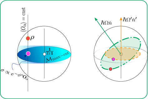
Figure 1:  Max-Ent dynamics in the Bloch’s sphere. Left: Max-Ent construction. The Max-Ent manifold ${\cal M}_{\textnormal{Max-Ent}}$ spans all the states with defined $\langle{\bf Q}_{x,y}\rangle=\langle{\bf S}_{x,y}\rangle$ mean values and maximum entropy. The state $\sigma$ is the state with maximum entropy that shares these averages with $\rho$. Right: the ideas of exact and Max-Ent dynamics are contrasted, where the latter is an approximation of the former.

Comment.

It is important to note that while $\mathfrak{C}_{B}(\mu_{\alpha})$ is generally a convex set, this is not necessarily true for ${\cal M}_{B}$ in general. In particular, if $S(\mathbb{H})$ represents the state space of a Spin-1 system and $B={{\bf S}_{x},{\bf S}_{y}}$, the states

$$\rho_{\mu=x,y}=\exp(-\ln(3){\bf S}_{\mu})/\Tr\exp(-\ln(3){\bf S}_{\mu})$$

belong to ${\cal M}_{B}$, while

$$\rho=\frac{1}{2}\rho_{x}+\frac{1}{2}\rho_{y}\propto e^{-\lambda({\bf S}_{x}+{\bf S}_{y})-\kappa\{({\bf S}_{x},{\bf S}_{y})\}-\xi{\bf S}_{z}{\bf S}_{z}}$$

with $\lambda\approx-0.526$, $\kappa\approx 0.137$, and $\xi\approx 0.125$ does not belong to ${\cal M}_{B}$, as it cannot be written in the form of Eq. 5.

I.2 Linear projections and geometry of ${\cal M}_{B}$

Evaluating ${\cal P}_{B}$ is, however, a challenging optimization problem, primarily due to the high computational cost associated with the exact evaluation of $\rho$. Nonetheless, in certain cases, our interest lies in projecting states $\rho\propto\exp(-{\bf K})$ onto the neighbourhood of a specific $\rho_{0}\propto\exp(-{\bf K}_{0})\in{\cal M}_{B}$. In such scenarios, it becomes reasonable to approximate $\Pi_{B}({\bf K})$ using a linear projector Amari and Nagaoka (2000); Walet and Klein (1990); Ignatyuk and Morozov (2019b),

$$\pi_{B}\left(\Delta{\bf K}\right)\equiv\pi_{B,{\bf K}_{0}}\left({\bf K}\right)=\left.\frac{\partial}{\partial\lambda}\Pi_{B}\left({\bf K}_{0}+\lambda\Delta{\bf K}\right)\right|_{\lambda\rightarrow 0}.$$ (9)

To explicitly construct $\pi_{B}$, observe that

$$\langle{\bf O}\rangle_{{\cal P}(\rho)}=\langle{\bf O}\rangle_{\rho},\quad\forall{\bf O}\in{\cal A}_{B}.$$ (10)

Assuming that $\rho\approx{\cal P}_{B}(\rho)\rightarrow{\bf K}\approx\Pi_{B}({\bf K})$ (i.e., the exact state of the system is in close proximity to the Max-Ent manifold), Eq. 10 can be linearized around ${\cal P}_{B}(\rho)$ using the following property:

Proposition 2.

Let $\rho_{\lambda}\propto\exp(-{\bf K}_{0}+\lambda\Delta{\bf K})$. Then,

$$\frac{\partial}{\partial\lambda}\langle{\bf O}\rangle_{\rho_{\lambda}}=({\bf O},\Delta{\bf K})_{\rho_{0}}^{\textnormal{{KMB}}},$$ (11)

with

$$({\bf Q}_{1},{\bf Q}_{2})_{\sigma}^{\textnormal{{KMB}}}=\int_{0}^{1}{\rm Tr}[\sigma^{1-\tau}{\bf Q}_{1}^{\dagger}\sigma^{\tau}{\bf Q}_{2}]d\tau.$$ (12)

the Kubo-Mori-Bogoliubov (KMB) scalar product Petz and Toth (1993) relative to $\rho_{0}$.

The proof of this proposition can be found in the work by Balian et al. (1986).

This condition allows us to characterize $\pi_{B}$ as an orthogonal projector with respect to the KMB product.

Proposition 3.

Eq. 9 is satisfied if $\pi_{B}$ is an orthogonal projection regarding $(\cdot,\cdot)^{\textnormal{KMB}}_{\rho_{0}}$, for all states $\rho_{0}\in{\cal M}_{B}$:

$$\bigg{(}{\bf Q},\pi_{B}({\bf O})\bigg{)}^{\textnormal{{KMB}}}=({\bf Q},{\bf O})^{\textnormal{{KMB}}}\;,\forall{\bf Q}\in{\cal A}_{B},{\bf O}\in{\cal A}.$$ (13)

A proof of this proposition can be found in Section A.3.

In a way, 3 implies that $\pi_{B}({\bf K})$ is the closest operator (in ${\cal M}_{B}$) to ${\bf K}$, w.r.t. the induced norm

$$||{\bf A}||_{\rho_{0}}^{\textnormal{KMB}}=\sqrt{({\bf A},{\bf A})_{\rho_{0}}^{\textnormal{KMB}}}\approx\frac{\partial}{\partial\lambda}S(e^{-{\bf K}_{0}}\|e^{-{\bf K}_{0}-\lambda{\bf A}})$$ (14)

On the other hand, it allows to write $\pi_{B}({\bf K})$ in terms of operators ${\bf Q}_{\alpha}\in B$ as a Bessel-Fourier expansion

$$\pi^{\textnormal{{KMB}}}_{B}({\bf K})=\sum_{\alpha\beta}({\cal G}^{\textnormal{{KMB}}^{-1}})^{\alpha\beta}({\bf Q}_{\alpha},{\bf K})^{\textnormal{{KMB}}}_{\sigma(t)}{\bf Q}_{\beta},$$ (15)

with

$${\cal G}_{\alpha\beta}^{\textnormal{{KMB}}}=({\bf Q}_{\alpha},{\bf Q}_{\beta})^{\textnormal{{KMB}}}_{\sigma(t)},\quad\sigma(t)\propto{\exp(-{\bf K}_{B}(t))}.$$ (16)

the Gram’s matrix of the basis of accessible observables w.r.t the KMB scalar product.

I.3 Projected dynamics and restricted dynamics

Now, let’s consider a system undergoing a closed evolution governed by the Schrödinger equation:

$${\bf i}\hbar\frac{d\rho}{dt}=[{\bf H},\rho],$$ (17)

where ${\bf H}\in{\cal A}$ represents the system’s Hamiltonian. For the present developments, it is convenient to work also with the equation for ${\bf K}(t)=-\log(\rho(t))$:

$${\bf i}\hbar\frac{d{\bf K}}{dt}=[{\bf H},{\bf K}],$$ (18)

Given that the accessible observables are limited to those in ${\cal A}_{B}={\rm span}(B)$, it is meaningful to examine the evolution of the projection:

$$\rho^{\textnormal{proj}}(t)_{B}={\cal P}_{B}(\rho(t))=\exp\big(-\Pi_{B}({\bf K}(t))\big{missing}),$$

which offers a more concise representation of the state with respect to the accessible observables. However, evaluating $\rho^{\textnormal{proj}}(t)_{B}$ necessitates solving the full Schrödinger equation 17 and subsequently computing the projection itself. This undermines the feasibility of employing a projection approximation.

Nevertheless, by assuming that $\rho(t)$ evolves in the neighborhood of ${\cal M}_{B}$, $\rho^{\textnormal{proj}}(t)_{B}$ can be approximated by a restricted evolution $\sigma(t)=\exp\big(-\tilde{{\bf K}}(t)\big{missing})$, where $\tilde{{\bf K}}(t)$ satisfies

$${\bf i}\hbar\frac{d\tilde{\bf K}}{dt}=\pi_{B}\big{(}[{\bf H},\tilde{\bf K}]\big{)},$$ (19)

representing a restricted Schrödinger evolution constrained to the Max-Ent manifold ${\cal M}_{B}$ Amari and Nagaoka (2000); Walet and Klein (1990); Ignatyuk and Morozov (2019b).

Using the orthogonal expansion Eq.15 regarding a fixed basis $B$, Eq.19 can be expressed as a set of differential equations for the expansion coefficients $\phi_{\mu}(t)$ (where $\tilde{\bf K}B(t)=\sum\mu\phi_{\mu}(t){\bf Q}_{\mu}$):

$$\sum_{\beta}{\cal G}_{\alpha\beta}^{\textnormal{{KMB}}}\frac{d\phi_{\beta}}{dt}=\sum_{\beta}{\cal H}^{\textnormal{{KMB}}}_{\alpha\beta}\phi_{\beta}(t),\$$ (20)

with

$${\cal H}_{\alpha\beta}^{\textnormal{{KMB}}}=\frac{1}{{\bf i}\hbar}({\bf Q}_{\alpha},[{\bf H},{\bf Q}_{\beta}])^{\textnormal{{KMB}}}_{\sigma(t)},$$ (21)

representing a matrix of real coefficients that govern the dynamics of the coefficients. It is important to note that both ${\cal H}_{\alpha\beta}$ and ${\cal G}_{\alpha\beta}$ are non-linear functions of the instantaneous ${\bf K}$, as $(\cdot,\cdot)_{B}^{\textnormal{KMB}}$ depends on $\exp\big(-\tilde{\bf K}_{B}(t)\big{missing})$. Consequently, Eq. 20 becomes a set of non-linear coupled equations.

Example

To illustrate how this approach works, let’s revisit the dynamics in the Bloch sphere. Consider $B={{\bf S}_{x},{\bf S}_{y}}$, and let the Hamiltonian have the form ${\bf H}=\check{n}\cdot\vec{\bf S}=\Omega{\bf S}_{z}+\omega{\bf S}_{x}$ (see Fig. 1 b). The exact dynamics describe circular trajectories around $\check{n}$ with an angular frequency of $\sqrt{\Omega^{2}+\omega^{2}}$. In this specific case, the natural projection over ${\cal M}_{B}$ (Eq. 10) coincides with the Euclidean projection onto the $x$-$y$ plane. If $\omega=0$, the projection of the exact trajectory onto ${\cal M}B$ coincides with the trajectory of the restricted dynamics. However, if $\omega\neq 0$, the restricted dynamics would still be a circular trajectory with an angular frequency of $\Omega$, while the projection of the exact dynamics would result in an elliptical trajectory with an angular frequency of $\sqrt{\Omega^{2}+\omega^{2}}$. When $|\omega/\Omega|\ll 1$, the restricted dynamics would closely approximate the projection of the exact dynamics. Furthermore, by choosing $B^{\prime}={\log\rho(0),-{\bf i}[{\bf H},\log\rho(0)]}$ instead of $B$, the dynamics would always be exact, despite $B^{\prime}$ being non-complete (although ${\cal A}{B^{\prime}}$ is closed).

Convergency

In the previous analysis, it was assumed that $\rho(t)\approx{\cal P}(\rho(t))$, in order to approximate the non-linear projector $\Pi_{B}$ by its linear approximation $\pi_{B}$. In general, along the evolution, the system develops correlations that are not contained in $B$. For example, in typical interacting many-body systems, an initially uncorrelated state develops ${\cal O}(t^{n})$ non-trivial $n$-body correlations. Then, if $B$ contains just single-particle observables, these correlations are neglected in the evolution of $\tilde{K}_{B}(t)$, while it does affect the dynamics of $\rho(t)$. Still, if these correlations do not affect the dynamics of the relevant expectation values in an appreciable manner, then $\exp\big(-\tilde{\bf K}_{B}(t)\big{missing})$ provides a good approximation to ${\cal P}(\rho(t))$, even if it does not approximate correctly $\rho(t)$. On the other hand, if the correlations do affect the dynamics of the relevant variables, it can be seen as the correlations are actually relevant observables, which can be inferred by looking at the dynamics of other observables.

This statement can be made exact by considering Hierarchical basis $B_{0}\subset B_{1}\subset B_{2}\subset\ldots\subset B_{L}\subset\ldots$ in a way that ${\bf K}(0)\in B_{0}$, and $[{\bf H},{\bf Q}]/({\bf i}\hbar)\in B_{L+1}\forall{\bf Q}\in B_{L}$. By considering $B_{L}$ as the relevant set, it is verified that $\|\pi_{B_{L}}{\bf K}(t)-{\bf K}(t)\|\propto t^{L}$.

II Computable general Max-Ent Dynamics

With the method above, in principle, it is possible to solve the projected dynamic for any choice of the physical system and set of relevant observables, involving just as many dynamical variables as the considered relevant independent observables. However, to explicitly solve the dynamics, the challenge lies in computing the self-consistent projections via the evaluation of the KMB scalar product of operators with respect to the instantaneous state $\sigma(t)$: its computation requires the construction and explicit diagonalization of the instantaneous state $\sigma(t)$ at each step of the evolution. This process can only be carried out explicitly for Gaussian and product states, and for very low-dimensional systems Vidal and Werner (2002).

One way to overcome this limitation arises from the observation that the same projector can be orthogonal regarding different scalar products. Moreover, even if two scalar products lead to different but similar orthogonal projectors, choosing a suitable basis $B$, it can be expected that the dynamic induced by the projectors will be similar. In this section, the desired requisites for a computable generalization of the KMB dynamics are discussed in depth, alongside a concrete proposal fulfilling these requisites.

II.1 Required properties.

In the upcoming sections, an alternative proposition to solve the Max-Ent projected dynamics equation Eq. 20 by replacing the KMB geometry with a mathematically similar yet computationally efficient geometry, is explored. To this end, one must, first, embark on a search for an alternative scalar product $(\cdot,\cdot)$ that can serve as a replacement for the KMB scalar product while possessing comparable metric properties. A comprehensive analysis of the mathematical properties of this scalar product can be found in Érik Amorim and Carlen (2020). Additionally, for a more extensive exploration of the broader applicability of this geometry, particularly from the perspective of operator theory, refer to the comprehensive summary provided in Balazs (2006). By pursuing this avenue, an improved approach for computing scalar products and orthogonalizing bases of observables with higher computational efficiency is desired. In order to achieve results similar to those obtained using the KMB scalar product, the proposed alternative must satisfy several significant conditions.

Reality condition.

Firstly, a suitable candidate of scalar product must meet the reality condition,

$$({\bf A},{\bf B})^{{}^{\prime}*}=({\bf A}^{\dagger},{\bf B}^{\dagger})^{\prime}=({\bf B}^{\dagger},{\bf A}^{\dagger})^{\prime}.$$ (22)

This condition ensures that $\pi_{B}({\bf Q})=\pi_{B}({\bf Q})^{\dagger}\in{\cal A}_{B}$ for any ${\bf Q}={\bf Q}^{\dagger}\in{\cal A}$ and any choice of $B$. Both the KMB scalar product and the Hilbert-Schmidt scalar product (HS), given by

$$({\bf A},{\bf B})^{\textnormal{HS}}=\Tr\mathbf{A}^{\dagger}{\bf B}$$

are real-valued scalar products Hall (2013).

Tensor-Product compatibility condition.

The HS scalar product is particularly advantageous as it is much easier to compute than the KMB scalar product when ${\bf A}^{\dagger}$ and ${\bf B}^{\dagger}$ represent $k$-body correlations. Furthermore, the HS scalar product is compatible with the tensor product operation:

$$({\bf O}_{1}\otimes{\bf O}_{2},{\bf Q}_{1}\otimes{\bf Q}_{2})_{\textnormal{HS}}=({\bf O}_{1},{\bf Q}_{1})({\bf O}_{2},{\bf Q}_{2}).$$ (23)

This property is not shared by the KMB product, even if $\sigma(t)$ is a product operator, which makes the evaluation of k-body correlation functions much harder than in the case of the HS case.

Statistical weight.

However, simple substitution of the KMB scalar product by the HS scalar product in Eq. 20 is not always a viable approach. The KMB scalar product assigns weights to operators based on their statistical significance, while the HS scalar product is unitarily invariant. As a result, two operators that are close in terms of the KMB-induced norm may appear very different according to the HS-induced norm. This discrepancy arises, for example, when the operators differ in the form $|i\rangle\langle j|$, with $|i\rangle$ and $|j\rangle$ being states with very low occupation probabilities ($\langle i|\rho|i\rangle,\langle j|\rho|j\rangle\ll 1$). For instance, in a bosonic system where $\hat{\bf n}={\bf a}^{\dagger}{\bf a}$ is the number operator and $\rho$ is a Gaussian state with $\langle n\rangle\approx 1$, $|\hat{\bf n}^{2}-\hat{\bf n}|_{\textnormal{KMB}}=2\sqrt{13}\approx 7.21$, but $|\hat{\bf n}^{2}-\hat{\bf n}|_{\textnormal{HS}}$ is unbounded.

II.2 Covariance inner product and Covariance geometry

A more suitable choice of scalar product is given by the covariance scalar product (w.r.t. a certain referene state $\sigma$),

$$({\bf O},{\bf Q})_{\sigma}^{\textnormal{(covar)}}=\rm Tr\left[\sigma\frac{\{{\bf O}^{\dagger},{\bf Q}\}}{2}\right],$$ (24)

which, for Hermitian inputs, is a real-valued scalar product.

This scalar product, up to a constant factor, reduces to the HS when $\sigma\propto\textnormal{id}_{\mathbb{H}}$. It has a simple statistical interpretation: the scalar product of an operator with the identity operator yields its expectation value,

$$({\bf id}_{\mathbb{H}},{\bf Q})_{\sigma}^{\textnormal{(covar)}}=\langle{\bf Q}\rangle_{\sigma},$$

while the scalar product between two operators with zero expectation value (i.e. orthogonal to the identity) is given by its covariance:

$$({\bf O},{\bf Q})_{\sigma}^{\textnormal{(covar)}}=\bigg{\langle}\frac{\{{\bf O},{\bf Q}\}}{2}\bigg{\rangle}_{\sigma},$$

In addition, the induced norm for an operator with zero expectation value is given by its standard deviation:

$$||{\bf Q}-\langle{\bf Q}\rangle||^{\textnormal{(covar)}}=\sqrt{\langle{\bf Q}^{2}\rangle-\langle{\bf Q}\rangle^{2}}.$$

Thus, the covariance scalar product can be regarded as the quantum analog of the covariance scalar product between classical random variables.

One notable advantage of the covariance scalar product, compared to the KMB geometry, is that it does not require diagonalizing the reference state for its computation, making it more computationally efficient. Furthermore, as it is a linear function w.r.t. the reference state, it can be efficiently computed for any separable reference state $\rho_{0}=\sum_{i}q_{i}\rho_{i}^{\otimes}$.

Moreover, althought it does not satisfy the tensor-product compatibility condition Eq. 24, for self-adjoint operators, it can be computed as the real part of the Gelfand-Naimark-Sigal (GNS) scalar product Hall (2013); Carlen and Maas (2020)

$$({\bf O},{\bf Q})_{\sigma}^{\textnormal{GNS}}={\rm Tr}[\sigma{\bf O}^{\dagger}{\bf Q}],$$

which does satisfy it. For example, by choosing $\sigma=\bigotimes_{i}\sigma_{i}$, the scalar product between ${\bf O}=\bigotimes_{i}{\bf o}_{i}$ and ${\bf q}=\bigotimes_{i}{\bf q}_{i}$ is simply given by

$$({\bf O},{\bf Q})_{\sigma}^{\textnormal{covar}}=\real\left[\prod_{i}({\bf o}_{i},{\bf q}_{i})_{\sigma_{i}}\right].$$

Apart from all these properties, COV shares with KMB a common orthogonal basis of ${\cal A}$, with the norms of each vector related by a ${\cal O}(1)$ factor (see Lemma 1 in Section A.2):

$$\big{(}|i\rangle\langle j|,|k\rangle\langle l|\big{)}_{\sigma}^{\textnormal{KMB}} = W_{ij}\times\big{(}|i\rangle\langle j|,|k\rangle\langle l|\big{)}_{\sigma}^{\textnormal{covar}},$$ (25)

$$W_{ij} = \frac{2\tanh(\log(p_{i}/p_{j})/2)}{\log(p_{i}/p_{j})}\leq 1$$ (26)

where $|i\rangle,|j\rangle,|k\rangle,|l\rangle$ are eigenvectors of $\sigma$ with eigenvalues $p_{i},p_{j},p_{k},p_{l}$ respectively. As a consequence, if $B\subset\{|i\rangle\langle j|\}$, the associated orthogonal projectors over ${\cal A}_{B}$ for $\pi\equiv\pi_{B}^{\textnormal{KMB}}$ and $\pi_{B}^{\textnormal{Covar}}$ are identical. On the other hand, in the general case, the following chain of inequalities holds

$$\|\pi^{\textnormal{KMB}}(\rho)\|^{\textnormal{KMB}} \leq \|\pi^{\rm(covar)}(\rho)\|^{\textnormal{KMB}}\leq\|\pi^{\rm(covar)}(\rho)\|^{\rm(covar)}$$ (27)

$$\leq \|\pi^{\textnormal{KMB}}(\rho)\|^{\rm(covar)}$$

which follows from Lemma 1 and the minimum distance property of the orthogonal projectors regarding the corresponding induced norm.

On the other hand, using the Parseval identity, it is straightforward to check that the distance between both projectors $\Delta_{\textnormal{KMB}}=\|\pi^{\textnormal{(covar)}}(\rho)-\pi^{\textnormal{KMB}}(\rho)\|^{KMB}$ is bounded by

$$\Delta_{\textnormal{KMB}} \leq \Delta_{\rm(covar)}$$ (28)

$$= \sqrt{(\|\pi^{\rm(covar)}(\rho)\|^{\rm(covar)})^{2}-(\|\pi^{\textnormal{KMB}}(\rho)\|^{\rm(covar)})^{2}}$$

$$\leq \|\pi^{\rm(covar)}(\rho)\|^{\rm(covar}$$

with $\Delta_{\rm(covar)}=\|\pi^{\rm(covar)}(\rho)-\pi^{\textnormal{KMB}}(\rho)\|^{\rm(covar)}$.

II.3 Connection with standard formulations of Mean Field Theory and equivalence of projections in the gaussian case

As shown in Section A.5, for some special choices of $B$, our formalism is equivalent to the (self-consistent) Time Dependent Mean Field Theory (TDMFT).

The simplest case is the one in which $\mathbb{H}=\mathbb{H}^{\otimes}$ and the basis $B$ of accessible observables is a basis of local observables

$$B=\bigsqcup_{i}B_{i},$$ (29)

with $B_{i}$ complete bases of the local algebras of operators ${\cal A}_{i}$ acting over $\mathbb{H}^{(i)}$. For this case, the formalism is equivalent to the Hartree (product-state based) mean field approach  Balian (1991); J. Uhlig et al. (1998); Bruus and Flensberg (2004); Matera et al. (2010).

In a similar way, if $\mathbb{H}=\mathbb{H}^{\textnormal{Fock}}$, and

$$B = B^{\textnormal{F}}_{1}\sqcup B^{\textnormal{F}}_{2}$$

$$B^{\textnormal{F}}_{1} = \{{\bf q}_{1},{\bf p}_{1},{\bf q}_{2},{\bf p}_{2},\ldots\}$$

$$B^{\textnormal{F}}_{2} = \{{\bf Q}\textnormal{ }|\textnormal{ }{\bf Q}=[{\bf z}_{i},{\bf z}_{j}]_{\mp}-\langle[{\bf z}_{i},{\bf z}_{j}]_{\mp}\rangle,\textnormal{ }{\bf z}_{i,j}\in{B}^{\textnormal{F}}_{1}\}$$

with ${\bf q}_{i}$, ${\bf p}_{i}$, observables s.t. $\langle{\bf p}_{i}\rangle=\langle{\bf q}_{i}\rangle=0$, satisfying canonical commutation/anti-commutation relations

$$[{\bf p}_{i},{\bf p}_{j}]_{\pm}=[{\bf q}_{i},{\bf q}_{j}]_{\pm}=0\;\;,[{\bf q}_{i},{\bf p}_{j}]_{\pm}={\bf i}\hbar\delta_{ij},$$

then our formalism is equivalent to the Time-Dependent Hartree-Fock-Bogoliubov (Gaussian-state based) Mean field theory Auerbach (1994); Ring and Schuck (2005). In both cases, the self-consistency condition – for the stationary case – is given by

$$\Pi_{\mathcal{M}_{B}}(\sigma)=\sigma\;,\;\langle{\bf H}\rangle=\langle\pi_{B}\left({\bf H}\right)\rangle.$$

In other words, for the bosonic Gaussian case, both geometries yield the exact same projection.

Possible simplifications using fixed referential mean-field states

While beyond the scope of this article, there exist further improvements that can be made to Eq. 20, besides altering the inner product. Specifically, instead of considering time-dependent scalar products w.r.t. the instantaneous state of the system, $\sigma(t)$, a single fixed and carefully chosen reference state $\sigma_{0}$ can be considered.

This proposal offers several advantages. For instance, by employing in Eq. 20 a covariance scalar product w.r.t. a fixed reference state $\sigma_{0}$, the resulting system of differential equations becomes linear. As a result, its solution becomes analytically tractable and numerically stable.

For this proposal to yield results comparable to the exact ones, the reference state $\sigma_{0}$ must exhibit a certain degree of similarity to the instantaneous states $\sigma(t)$ throughout the evolution. One way to achieve this is by considering a mean-field state as the reference state, i.e. $\sigma_{0}$ must be chosen s.t.

$$\pi^{\textnormal{MF}}(\sigma_{0})=\sigma_{0},$$

where $\pi^{\textnormal{MF}}:{\cal A}\rightarrow{\cal A}_{B}$ is the Mean-Field projector for the relevant basis of observables $B$. These ideas are discussed in depth in Section A.5. In the upcoming sections, these ideas will not be employed, and the scalar scalar product will be computed w.r.t. the instantaneous state of the system.

III Test Example

By replacing the KMB scalar product with the correlation scalar product as depicted in Eq. 16, one can derive expressions completely analogous to those presented Eq. 20 and Eq. 21, albeit w.r.t. the aforementioned alternative scalar product. Although the correlation scalar product exhibits mathematical similarity to the KMB scalar product and offers computational advantages, it remains to be seen whether it yields accurate results, when compared to both exact outcomes and those obtained through the KMB geometry. These ideas will be tested on a simple physical system, specifically the one-dimensional Heisenberg spin-$\frac{1}{2}$ chain, which will be summarized in the subsequent section. The objective is, then, to compare the exact results, obtained through numerical solutions of the Schrödinger equation Eq. 17, with those derived from the KMB geometry and the geometry induced by the correlation scalar product.

III.1 XX Heisenberg Model

As an illustrative instance of the preceding formalism, let us contemplate a spin-$\frac{1}{2}$ nearest-neighbour Heisenberg XX model on a periodic chain one-dimensional lattice composed of $N$ sites. The system is governed by a Hamiltonian, given by:

$${\bf H}=-J\bigg{(}\sum_{j=1}^{N}{\bf S}_{j}^{x}{\bf S}_{j+1}^{x}+{\bf S}_{j}^{y}{\bf S}_{j+1}^{y}\bigg{)}$$ (30)

s.t. ${\bf S}_{N+1}^{x,y,z}\equiv{\bf S}_{1}^{x,y,z}$ and where $\{{\bf S}_{j}^{x},{\bf S}_{j}^{y},{\bf S}_{j}^{z}\}$ are the usual spin-$\frac{1}{2}$ operators and where $J$ is the strength of the flip-flop term ${\bf S}_{j}^{x}{\bf S}_{j+1}^{x}+{\bf S}_{j}^{y}{\bf S}_{j+1}^{y}$. Note that the ${\bf S}_{n}^{x,y,z}$ operators act non-trivially just on the $n$-th site. This state of the system can be described using (linear combinations of) tensor products of $N$ $\mathfrak{s}\mathfrak{u}(2)$ representations, with the identity operator, added for each lattice site. Its Hilbert space is $2^{N}$-dimensional, where one possible configuration is $\ket{\uparrow_{1}\uparrow_{2}\cdots\downarrow_{N}}$. In a quantum information context, these states are known as the computational basis vectors. Moreover, both the XX and the more general, XY model can be analytically diagonalized via a Jordan-Wigner transformation Jordan and Wigner (1928); Lieb et al. (1961). However, computing time-dependent numerical correlations, which are important for understanding these model’s low-temperature behaviour -amongst other important physical features- Hansson et al. (2017); Lee (2007), requires a numerical computation, wherein the previous technological difficulties readily become apparent.

Observables and quantum numbers

Since the total magnetization ${\bf S}^{z}_{T}=\sum_{i}{\bf S}_{i}^{z}$ commutes with the Hamiltonian, all states may be labelled with an additional quantum number, indicating the total number of excitations present in a given configuration, relative to the reference state Auerbach (1994)

$$|\downarrow\downarrow\ldots\rangle\equiv|0\rangle.$$

Furthermore, the magnetization is a conserved quantity and, hence, the Schrödinger evolution preserves it, i.e. a state with $n$ excitations will evolve in time to states with exactly $n$ excitations, as well.

Consider, then, the following operator, basically a redefinition of the global magnetization,

$${\bf n}=\sum_{j=1}^{N}\bigg{(}{\bf S}^{z}_{j}+\frac{1}{2}\bigg{)}.$$ (31)

This operator, the occupation operator, measures how many flipped excitations the system contain, w.r.t to the reference state $|\downarrow\downarrow\ldots\rangle$, and is a constant of motion. In particular, consider a system with initial state $\rho_{0}$ s.t. $\langle\hat{\bf n}\rangle_{\rho_{0}}=1$, undergoing a Schrödinger evolution. Then, $\langle\hat{\bf n}\rangle_{\rho(t)}=1$ at all times.

A second quantum number of interest is the average (normalized) localization of the excitations, given by a position operator

$${\bf x}=\sum_{j=1}^{N}\bigg{(}2\frac{j-1}{N-1}-1\bigg{)}\bigg{(}{\bf S}^{z}_{j}+\frac{1}{2}\bigg{)},$$ (32)

which measures which lattice site contains the excitation. This accessible observable will be of relevance in the following section.

III.2 Numerical Exploration of the projected dynamics

Thus far, two potential alternatives for dynamics involving projections have been introduced. In the rest of this section, the projected and restricted evolutions are going to be compared. The former are derived by projecting the exact dynamics onto the Max-Ent manifold, as described in equation Eq. 15. On the other hand, the restricted evolutions are obtained by solving the equation of motion, as stated in equation Eq. 20, utilizing different types of linear projectors $\pi^{s}$ with $s=\textnormal{KMB}/\textnormal{covar}$. This also serves to gauge how well justified is the hypothesis of substituing the KMB geometry by the covariance geometry.

III.2.1 Projected Evolutions

Consider a six-site XX chain, whose Hilbert space $\mathbb{H}^{\otimes}=\otimes_{j}\mathbb{H}^{(j)}$ is 64-dimensional, high-dimensional enough for exact numerical methods to be applicable but cumbersome and computationally expensive as well. In order to quantify how well the KMB and correlation geometries perform in simulating exact results for this particular physical system, the exact dynamics will be projected, using the the KMB and covariance projectors and. Said results will be used to compare several quantities of interest. Numerical computations are computed using Quantum Toolbox in Python’s (QuTip) function master equation solver Johansson et al. (2013).

Initial Conditions

In this article, all physical quantities are in natural units, i.e. ${\hbar=1}$. This section’s discussion is restricted to a ferromagnetic XX model with coupling strength $J=1$ in the absence of a magnetic field,, with closed boundary conditions.

Next, the initial state of the system $\rho_{0}=\rho(0)$ is chosen to lie in the Max-Ent manifold and is given by

$$\begin{split}\rho(0)&\propto e^{-{\bf K}(0)},\\ &{\bf K}(0)=\beta{\bf H}+c_{1}(\hat{\bf n}-\zeta)^{2}+c_{2}(\hat{\bf x}-{\bf x}_{0})^{2},\end{split}$$ (33)

where $\beta$ is the inverse temperature. Two values of $\beta$ are of interest: $\beta=J$ and $\beta=J/10$. Here, $\rho(0)$ is a Max-Ent state regarding the observables ${\bf H},{\bf n},{\bf n}^{2},{\bf x},{\bf n}^{2}$. The other coefficients are chosen s.t. $\langle\hat{\bf n}\rangle_{\rho_{0}}\approx 1$. In the first case, $c_{1}=3\beta,c_{2}=3\beta,\zeta=1$ and $x_{0}=-.3$ have been chosen, while in the second case, $c_{1}=10\beta,c_{2}=10\beta,\zeta=1$ and $x_{0}=-.3$.

Moreover, the basis $B$ of observables of interest takes on a very particular form, in terms of iterated commutators between the $\hat{\bf H}$ and the ${\bf K}_{0}$ operators. In particular, consider

$$\begin{split}&B_{L}=B_{0}+B^{it}_{L},\\ &B_{0}=\{\textnormal{id}_{\mathbb{H}},{\bf n},{\bf n}^{2},{\bf x},{\bf x}^{2},{\bf K}_{0}\}\\ &B^{it}_{L}=\{\underbrace{[{\bf H}_{0},{\bf K}_{0}]/({\bf i}),\big{[}{\bf H}_{0},[{\bf H}_{0},{\bf K}_{0}]\big{]}/({\bf i})^{2},\cdots}_{\textnormal{a total of $L$ times}}\}\end{split}$$ (34)

For this system, it was considered the case $B=B_{4}$.

Geometric distance between projections

In this section, a comparison is presented between the geometric distance of the logarithms of the exact states and the logarithms of the states derived from the KMB- and correlation-projections. The correct distance on the Max-Ent manifold, as previously discussed, is given by the KMB-induced norm w.r.t. the instantaneous state. The logarithms of the exact states ${\bf K}(t)=-\log\rho(t)$ are obtained from (numerically) solving the (free) Schrödinger equation on the ${\bf K}$ operator, Eq. 18. Next, these ${\bf K}$-states are projected, w.r.t to the fixed basis $B$ of observables given by Eq. 34, using the KMB- and the covariance scalar products (see Eq. 15, yielding the ${\bf K}$-states labelled ${\bf K}_{\textnormal{KMB}}(t)$ and ${\bf K}_{\textnormal{corr}}(t)$, respectively. With these objects, one can compute the KMB-induced distances between:

• the exact and the KMB-projected ${\bf K}$-states,

  $${||{\bf K}_{\textnormal{exact}}-{\bf K}_{\textnormal{KMB}}||^{\textnormal{KMB}}_{\rho(t)}}.$$

• the exact and the correlation-projected ${\bf K}$-states,

  $${||{\bf K}_{\textnormal{exact}}-{\bf K}_{\textnormal{covar}}||^{\textnormal{KMB}}_{\rho(t)}},$$

• and, finally, between the KMB-projected and correlation-projected ${\bf K}$-states,

  $${||{\bf K}_{\textnormal{KMB}}-{\bf K}_{\textnormal{covar}}||^{\textnormal{KMB}}_{\rho(t)}},$$

The results pertaining to both temperatures are depicted in Fig. 2. It is evident from the data that, for short-term evolutions, all three evolutions exhibit minimal, albeit non-zero, differences. However, as the evolutions extend to longer durations, the discrepancy between the projected states and the exact states increases, eventually reaching a saturation point at around the $t/J\simeq 10$ mark. In contrast, the geometric distance between the correlation- and KMB- ${\bf K}$-states remains very small during the entirety of the simulation. In general, one notes that the projected states remain in close proximity to the exact states, albeit at a growing distance. These observations support our proposal of substituing the computationally-expensive KMB geometry by the covariance geometry.

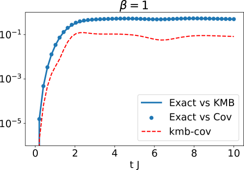
(a)

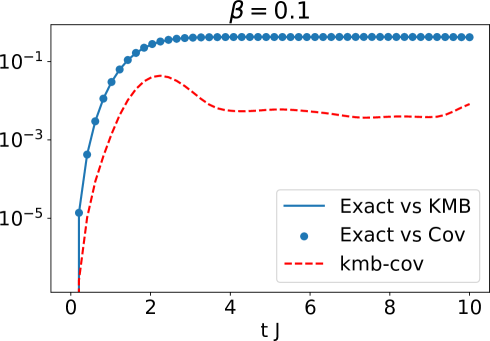
(b)

Figure 2: The figures presented herein, illustrate the KMB-induced norms between the exact logarithm of the density states and their KMB/correlation projections, in logarithmic scale, obtained from a $T<10/J$ simulation with 200 steps. It is evident from the data that, for short-term evolutions, both the KMB and correlation projected geometries exhibit remarkable similarity amongst themselves and with the exact state.

Time evolution of Expected Values

Our focus, now, shifts to examining the temporal evolution of the expected values associated with two specific operators of interest: the occupation operator ${\bf n}$ and the position operator ${\bf x}$. The aim is, now, to compute these expected values from the aforementioned three distinct frameworks: (1) the exact states $\rho(t)$, and (2) the states arising from the KMB/correlation projections, namely $\sigma_{\textnormal{KMB}}$ / $\sigma_{\textnormal{covar}}$, respectively. The states $\sigma_{\textnormal{KMB}}$ and $\sigma_{\textnormal{covar}}$ are obtained by exponentiating ${\bf K}_{\textnormal{KMB}}(t)$ and ${\bf K}_{\textnormal{covar}}(t)$, respectively, followed by normalization. Through the evaluation of the expected values of the ${\bf n}$ and ${\bf x}$ operators w.r.t these states, comparisons between the different evolutions can be made.

In Fig. 3, and Fig. 4 the time evolutions of the expected values associated with the occupation ${\bf n}$ and position ${\bf x}$ operators respectively, are depicted. These plots correspond to a simulation of $t=10/J$ of duration, employing a grid of 200 points.

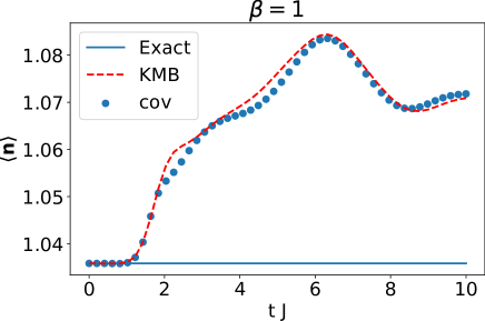
(a)

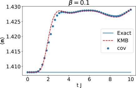
(b)

Figure 3: The figures presented depict the expected values of the occupation operator $\hat{\hat{\bf n}}$ at two distinct temperatures. It is evident from the data that, for short-term evolutions lasting less than $t/J=2$, all three frameworks yield highly similar outcomes, with discernible differences beginning to emerge thereafter.

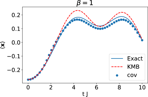
(a)

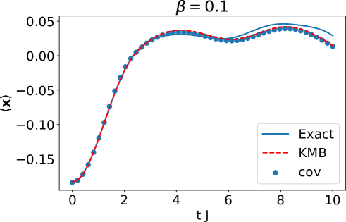
(b)

Figure 4: The figures presented illustrate the expected values of the position operator $\hat{\bf x}$ at two different temperatures, $\beta=1$ (top) and $\beta=0.1$ (bottom). Interestingly, it can be observed that all three frameworks yield remarkably similar results, with no major differences discernible among them.

From Fig. 3, it is evident that the expected values of the occupation operator remain approximately constant over time, which is consistent with it being a conserved quantity. Fluctuations on the projected evolution are due to the fluctuations in the normalization of the state. Interestingly, before the $t/J=1$ mark, all three frameworks exhibit highly similar outcomes, indicating a strong agreement between the projected and exact frameworks. However, as the simulation progresses, discrepancies between the projected and exact frameworks become more pronounced and eventually reach a saturation point around the $t/J=10$ mark. Notably, the difference between the KMB- and cov projections remains minimal, throughout the entire evolution. This finding is particularly encouraging, as it highlights the favourable performance of the correlation scalar product. Furthermore, regarding the time evolution of the expected value of the position operator, as depicted in Fig. 4, it is even more promising that all three frameworks consistently produce similar results throughout the simulation, with barely discernible differences observed among them.

Relative Entropies

Finally, we are interested in quantifying relative entropies between the exact free evolution and both kind of projections. In particular, the following relative entropies are of interest:

1. the relative entropy between the exact and the KMB-projected states, $S(\rho||\sigma_{\textnormal{KMB}})$,

2. the relative entropy between the exact and the correlation-projected states, $S(\rho||\sigma_{\textnormal{covar}})$,

3. and both types of relative entropies between the correlation- and KMB-projected states, $S(\sigma_{\textnormal{covar}}||\sigma_{\textnormal{KMB}})$ and $S(\sigma_{\textnormal{KMB}}||\sigma_{\textnormal{covar}})$.

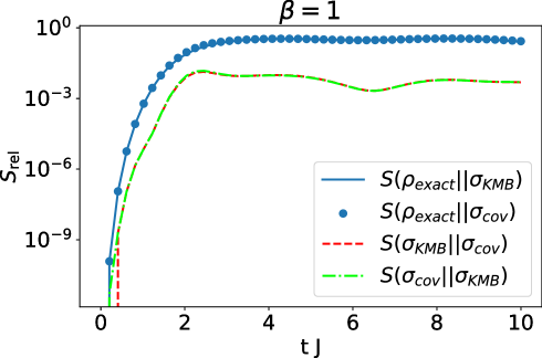
(a)

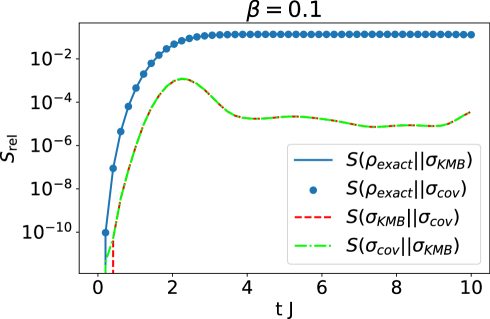
(b)

Figure 5: The figures presented herein show, in logarithmic scale, the relative entropies between exact and projected density states, for two different temperatures. Once again, for short-term evolutions, the three frameworks yield very similar results. For longer-term evolutions, the relative entropies saturates.

In Fig. 5, the evolution of the relative entropies are depicted for two different temperatures. Consistent with the findings presented in Fig. 2, it can be observed that for short-term evolutions, the relative entropies between different states exhibit very small values, indicating a high level of similarity among these states. However, for larger times, the relative entropies between the exact and projected states become more noticeable, eventually reaching a saturation point. This behavior aligns closely with the trends observed in the geometric distances between the three classes of states, as shown in Figure 2. Furthermore, it is worth noting that the relative entropies between the KMB-projected and correlation-projected states remain consistently negligible throughout the entire evolution, further underscoring the strong agreement between these two frameworks.

III.3 Projected vs Restricted dynamics

So far, the comparison was focused on the exact (free) dynamic and its KMB and cov projections over the Max-Ent manifold. Let’s compare now them against the solutions to the restricted equation of motion (see eq. 20) obtained from the KMB and cov instantaneous projections, computed by means of the orthogonal expansion Eq. 15.

Numerically solving equation Eq. 20 presents significant challenges even for not-too-high-dimensional systems due to the high computational cost associated with the KMB geometry. For this reason, it was considered a smaller chain, comprising just four sites. As before, the initial state of the system was chosen with form described in equation Eq. 33, but with parameters $\beta=5\times 10^{-1}$ and $c_{1}=2.5$, $c_{2}=5$, $\zeta=1$, and $x_{0}=0.19$, in a way that $\langle{\bf n}\rangle_{\rho_{0}}\approx 1$.

The projected and restricted evolutions were implemented using a basis of the form Eq. 34 with $L=3$.

While not addressed in depth in this article, it is worth mentioning that both the covariance-restricted and KMB-restricted evolutions could be enhanced in terms of computational efficiency by approximating the instantaneous reference state with product states by means of a mean field approximation of the instantaneous state. Additionally, the covariance scalar product enables the introduction of additional correlations using separable states as reference states. These approximations could allow us to solve much larger problems without significant overhead. However, the aim here is to compare the effect of the different choices of projections, which could be masked by these further simplifications.

Fig. 6 illustrates the KMB-induced norm between the state of the system (top) and the expectation value of the ${\bf x}$ operator (bottom) for both the exact and projected dynamics and the KMB/covariance restricted dynamics.

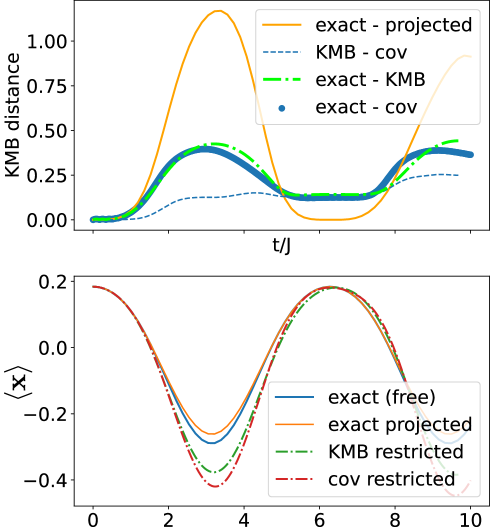
Figure 6: This figure depicts a comparison of the KMB-induced distance between the state, the projected state and the state arising from the restricted evolution and the expectation value of the ${\bf x}$ operator, according to the KMB and covariance geometries. For short-term evolutions, it is evident that all evolutions yield comparable results.

As is expected, for short times, the exact, free dynamic is asymptotically close to both the KMB projected and the restricted dynamics, disregarding the choice of the projectors. For longer times, the behavior of the restricted projections is similar among them, being sometimes closer to the exact (free) dynamic than the (linearly) projected evolution. This happens in particular when the distance between the exact state and its projection is relatively large: when this happens, the linear projection $\pi_{B}$ does not provide a good approximation to the Max-Ent projection ${\cal P}_{B}$, giving the restricted dynamics a better approximation.

Similar conclusions can also be drawn concerning the expectation value of the position operator: In this case, the projected dynamic reproduces its behavior more closely than the restricted evolutions, both in phase and amplitude. Nevertheless, the estimations from the restricted evolutions are still qualitatively good, and very similar among them.

IV Conclusions

This article introduced a quantum generalization of the covariance scalar product, originally defined for classical random variables, and compared it against the KMB scalar product in the context of estimating the Max-Ent projection for the dynamics of closed quantum systems. The covariance scalar product demonstrated a significant computational advantage over the KMB scalar product, making it a more efficient choice.

Through a case study on the one-dimensional XX Heisenberg model, it was observed that the restricted Max-Ent dynamics obtained from both the KMB and covariance-induced projections were close. Moreover, these projections were closer to each other than to the state obtained from free evolution or its Max-Ent linearized projection.

These findings suggest that while the KMB orthogonal projection represents the actual, consistent local linearization of the Max-Ent projection, the covariance orthogonal projection can yield similar results with less computational cost. To make this approach suitable for efficient quantum simulations of larger quantum systems, the next step would involve replacing the reference states with more efficient approximations of the instantaneous states. Exploring such alternatives is the focus of our upcoming work, currently in preparation.

V Acknowledgments

The authors would like to thank Joaquín Pelle for interesting discussions on the topology of quantum manifolds, Matías Bilkis for useful remarks about this work, Tomás Crosta for interesting discussions concerning the numerical aspects of our work, as well. The authors acknowledge support from CONICET of Argentina. Work supported by CONICET PIP Grant No. 11220200101877CO.

Appendix A Proofs

A.1 Proof of 1

To provide a self-contained presentation, in this section, a proof of 1, which can be found in other references (see for instance Jaynes (1957a); Balian (1991), is reproduced.

Proof.

Given that $\sigma^{\star}\in{\cal B}(\mathbb{H})$, an open set, and given that both the target function and the constraints are continuous, differentiable functions, $\sigma^{\star}$ must satisfy the stationary condition,

$$\delta\left.\bigg{(}S(\sigma)-\sum_{\alpha=0}^{N}\lambda_{\alpha}C_{\alpha}(\sigma)\bigg{)}\right|_{\sigma=\sigma^{\star}}=0,$$

where $\mu_{\alpha}$ are Lagrange multipliers, and where the $C_{\alpha}(\sigma)={\rm Tr}\sigma{\bf Q}_{\alpha}-\mu_{\alpha}=0$ are the constraints that define $\mathfrak{C}_{B}(\mu_{\alpha})$. For simplicity, ${\bf Q}_{0}={\mathbf{id}_{\mathbb{H}}}$ is included in $\mathcal{A}$, in a way that the normalization of $\sigma$ is fixed by taking $\langle{\mathbf{id}_{\mathbb{H}}}\rangle=1$. Notice again, however, that ${\bf Q}_{0}$ is not a true observable.

Using the identity

$$\langle i|\delta\log(\sigma)|j\rangle=\frac{\log(p_{i})-\log(p_{j})}{p_{i}-p_{j}}\langle i|\delta\sigma|j\rangle,$$

where $\sigma=\sum_{i}p_{i}|i\rangle\langle i|$, it follows that

$$\delta S(\sigma)=-{\rm Tr}\delta\sigma\log(\sigma)-{\rm Tr}\delta\sigma,$$

and hence,

$$\left.-{\rm Tr}\left[\delta\sigma\left(\log(\sigma)+(\lambda_{0}+1)+\sum_{\alpha=1}^{N}\lambda_{\alpha}{\bf Q}_{\alpha}\right)\right]\right|_{\sigma=\sigma^{\star}}=0$$

As a result, it follows that

$$\sigma^{\star}=e^{-{\bf K}-(\lambda_{0}+1)}=\frac{e^{-{\bf K}}}{\Tr e^{-{\bf K}}},$$

with ${\bf K}=\sum_{\alpha=1}^{N}\lambda_{\alpha}{\bf Q}_{\alpha}\in{\cal A}_{B}$ and $\lambda_{0}=\log(\Tr e^{-{\bf K}})-1$ to fix the normalization.

∎

A.2 Spectral norm and induced norm inequalities

Lemma 1.

$\|{\bf A}\|\geq||{\bf A}||^{\textnormal{covar}}_{\sigma}\geq||{\bf A}||^{\textnormal{KMB}}_{\sigma}$

Proof.

The first inequality is a direct consequence of the spectral norm definition and the spectral decomposition of $\sigma=\sum_{k}p_{k}|k\rangle\langle k|$:

$$(||{\bf A}||^{\textnormal{covar}}_{\sigma})^{2} = \Tr\sigma\textnormal{ }\frac{{\bf A}^{\dagger}{\bf A}+{\bf A}{\bf A}^{\dagger}}{2}$$

$$= \sum_{k}p_{k}\frac{\langle k|{\bf A}^{\dagger}{\bf A}|k\rangle}{2}+\sum_{k}p_{k}\frac{\langle k|{\bf A}^{\dagger}{\bf A}|k\rangle}{2}$$

$$\leq \sum_{k}p_{k}\frac{\|{\bf A}\|^{2}+\|{\bf A}^{\dagger}\|^{2}}{2}$$

$$= \sum p_{k}\|{\bf A}\|^{2}=\|{\bf A}\|^{2}$$

As to the second inequality, it is enough to show that ${\cal G}^{\textnormal{KMB}}_{\sigma}\leq{\cal G}^{\textnormal{covar}}_{\sigma}$. Also, as both matrices are diagonal in the canonical basis associated with the eigenvectors of $\sigma$, it is enough to show that

$$\bigg{(}||\textnormal{ }\ket{i}\bra{j}\textnormal{ }||^{\sigma}_{\textnormal{KMB}}\bigg{)}^{2} \leq \bigg{(}||\textnormal{ }\ket{i}\bra{j}\textnormal{ }||^{\sigma}_{\textnormal{covar}}\bigg{)}^{2}$$ (35)

or, in terms of the eigenvalues $p_{i}$ of $\sigma$,

$$\frac{(p_{i}-p_{j})/\log(p_{i}/p_{k})}{(p_{i}+p_{j})/2}\leq 1$$

Now, without lost of generality, let’s assume that $p_{i}\geq p_{j}$ and hence, $\log(p_{i}/p_{j})=x\geq 0$. Then,

$$\frac{(p_{i}-p_{j})/\log(p_{i}/p_{k})}{(p_{i}+p_{j})/2} = \frac{1-e^{-x}}{x/2(1+e^{-x})}$$

$$= \frac{\tanh(x/2)}{x/2}\leq 1$$

∎

A.3 The $\pi_{B}$ projector is an orthogonal projector w.r.t. the KMB scalar product

Proof.

From the condition Eq. 10, if follows that for any ${\bf Q}\in B$,

$${\rm Tr}\bigg{[}{\bf Q}\textnormal{ }\frac{d}{dt}\Pi_{{\cal M}_{B}}(\rho)\bigg{]}={\rm Tr}\bigg{[}{\bf Q}\textnormal{ }\Pi_{{\cal M}_{B}}\frac{d}{dt}\rho(t)\bigg{]}={\rm Tr}\bigg{[}{\bf Q}\textnormal{ }\frac{d}{dt}\rho(t)\bigg{]},$$

and, if ${\bf K}(t)=\log\rho(t)$, $\tilde{{\bf K}}(t)=\log\Pi_{{\cal M}_{B}}\rho(t)$, and using that $\rho(0)=\Pi_{\mathcal{M}_{B}}\rho(0)$,

$$\int{\rm Tr}{\bf Q}\rho(0)^{\tau}\frac{d{\bf K}}{dt}\rho(0)^{1-\tau}d\tau=\int{\rm Tr}{\bf Q}\rho(0)^{\tau}\frac{d\tilde{\bf K}}{dt}\rho(0)^{1-\tau}d\tau$$

or, in terms of the KMB scalar product,

$$\left.\bigg{(}{\bf Q},\frac{d}{dt}{\bf K}\bigg{)}_{\rho(0)}^{\textnormal{KMB}}\right|_{t=0}=\left.\bigg{(}{\bf Q},\frac{d}{dt}\tilde{\bf K}\bigg{)}_{\rho(0)}^{\textnormal{KMB}}\right|_{t=0}$$

Now, using the condition Eq. 9,

$$\left.\bigg{(}{\bf Q},\frac{d}{dt}{\bf K}\bigg{)}_{\rho(0)}^{\textnormal{KMB}}\right|_{t=0}=\left.\bigg{(}{\bf Q},\pi_{B}\textnormal{ }\frac{d}{dt}{\bf K}\bigg{)}_{\rho(0)}^{\textnormal{KMB}}\right|_{t=0},$$

which should hold for any possible evolution $\frac{d{\bf K}}{dt}=[{\bf H},{\bf K}(0)]/({\bf i}\hbar)={\bf K}^{\prime}\in{\cal A}$. As a result, Eq. 9 implies that $\pi_{B}$ is an orthogonal projection regarding the KMB scalar product. ∎

A.4 KMB and correlation scalar product in the gaussian case

If $\sigma$ is a (bosonic or fermionic) Gaussian state, it is possible to choose a basis for the quadratic forms on creation and anihilation operators, ${\bf a}_{i}$, ${\bf a}^{\dagger}_{i}$, satisfying canonical commutation (anticommutation) relations $[{\bf a}_{j},{\bf a}_{j}]_{\pm}=[{\bf a}_{i}^{\dagger},{\bf a}_{j}]_{\pm}=0$ and $[{\bf a}_{i},{\bf a}^{\dagger}_{j}]_{\pm}=\delta_{ij}$ s.t.

$$\begin{split}&\langle{\bf a}_{i}\rangle=\langle{\bf a}^{\dagger}_{i}\rangle=0,\quad\langle{\bf a}^{\dagger}_{i}{\bf a}^{\dagger}_{j}\rangle=\langle{\bf a}_{i}{\bf a}_{j}\rangle=0,\\ &\langle{\bf a}^{\dagger}_{i}{\bf a}_{j}\rangle=\delta_{ij}n_{j},\end{split}$$

with $n_{j}=({e^{\Omega_{j}}-\zeta})^{-1}$, $\zeta=\pm 1$ for the bosonic and fermionic case, respectively. With these operators thus defined, the basis $B^{\prime}=\{{\bf id}_{\mathbb{H}},{\bf a}_{i},{\bf a}_{i}^{\dagger},{\bf a}_{i}{\bf a}_{j},{\bf a}_{i}^{\dagger}{\bf a}_{j}^{\dagger},{\bf a}_{i}^{\dagger}{\bf a}_{j}-\delta_{ij}n_{i},\}$ provides an orthogonal basis w.r.t. both the KMB and correlation scalar products. These products differ only on the induced norm over the operators, as it is shown in table Table 1.

Using this property, it is straightforward to span the projector as

$$\pi({\bf O})=\sum_{{\bf Q}\in B}\frac{({\bf Q},{\bf O})^{s}}{({\bf Q},{\bf Q})^{s}}{\bf Q}$$

where $s={\rm KMB/covar}$ and where $\pi$ the orthogonal projector w.r.t the scalar product $(\cdot,\cdot)^{s}$.

	KMB	covar
${\bf id}_{\mathbb{H}}$	1	1
${\bf a}_{i}$	${1}/{\Omega_{i}}$	$n_{i}$
${\bf a}_{i}{\bf a}_{j}$	$\frac{1+n_{i}+n_{j}}{\Omega_{i}+\Omega_{j}}$	$n_{i}n_{j}+\frac{n_{i}+n_{j}+1}{2}$
${\bf a}^{\dagger}_{i}{\bf a}_{j}$	$\frac{n_{j}-n_{i}}{\Omega_{i}-\Omega_{j}}$	$n_{i}n_{j}+\frac{n_{i}+n_{j}}{2}$
${\bf a}^{\dagger}_{i}{\bf a}_{i}-n_{i}$	$n_{i}(n_{i}+1)$	$n_{i}(n_{i}+1)$
${\bf a}^{2}_{i}$	$\frac{1/2+n_{i}}{\Omega_{i}}$	$2(n_{i}+1/2)^{2}+1/2$

Table 1: Induced norms for the KMB and the correlation scalar products for the elements of the basis $B^{\prime}$. Here, $i\neq j$, and the last line just applies for bosons.

A.5 MFA and Gaussian-state-based MFT as Max-Ent dynamics

Standard mean field treatment for composite quantum systems, both in the case of product-state-based and gaussian-state based versions, can be stated in terms of Max-Ent projections. In the product-state case, the subspace ${\cal A}_{B}$ is defined by the local operators, in a way s.t. $B=\bigsqcup_{i}B_{i}$, wherein the $A_{B_{i}}$ sets define closed subalgebras of ${\cal A}$. The Max-Ent states are, then, product states $\rho=\bigotimes_{i}\rho_{i}$. Moreover, general operators ${\cal O}\in{\cal A}$ can be written as linear combinations of products of local operators, with their expectation values written in terms of products of local expectation values. In this way, for product states, the expectation value of any observable is a functional of the expectation values of an independent set of local observables.

On the other hand, for gaussian-state-based MFT (both for the bosonic and the fermionic cases), ${\cal A}_{B}$ is the sub-algebra of quadratic forms in creation and annihilation operators, making the Max-Ent states Gaussian states. Thanks to the Wick’s theorem, expectation values can be written as linear combinations of products of expectation values of operators in $B$.

In both cases, the projection $\pi^{\textnormal{MF}}:{\cal A}\rightarrow{\cal A}_{B}$ can be written as

$$\pi_{\sigma}^{\textnormal{MF}}({\bf O})=\sum_{{\bf Q}\in B}({\bf Q}-\langle{\bf Q}\rangle_{\sigma})\frac{\partial\langle{\bf O}\rangle_{\sigma}}{\partial\langle{\bf Q}\rangle_{\sigma}}+\langle{\bf O}\rangle_{\sigma},$$ (36)

with mean values evaluated regarding $\sigma\in{\cal M}_{B}$. The self-consistency equation for the stationary case can be written as

$$\sigma=\frac{\exp(-\pi_{\sigma}^{\textnormal{MF}}({\bf H}))}{\Tr\exp(-\pi_{\sigma}^{\textnormal{MF}}({\bf H}))},$$ (37)

while the time-dependent equations can be written as

$$\frac{d{\bf K}}{dt}=\pi_{\sigma}^{{\textnormal{MF}}}\left(\frac{[{\bf H},{\bf K}]}{{\bf i}\hbar}\right).$$

We claim the following,

Proposition 4.

$\pi^{\textnormal{MF}}$ represents an orthogonal projection regarding both the KMB and the correlation scalar product.

It is convenient, first, to consider some special basis of operators which simplifies the analytical evaluation of expansions and scalar products. In particular, for product state based MFT, $\sigma=\bigotimes_{i}\sigma_{i}$, we are going to use the local basis

$$B_{i}=\bigg{\{}\bigg{(}|\alpha\rangle\langle\alpha^{\prime}|-\langle\alpha^{\prime}|\alpha\rangle\frac{{\bf id}_{{(i)}}}{\Tr\mathbf{id}_{{(i)}}}\bigg{)}\otimes{\bf id}_{\overline{i}}\bigg{\}},$$

with $|\alpha\rangle$, $|\alpha^{\prime}\rangle$ orthogonal eigenvectors of $\sigma_{i}$, ${\bf id}_{i}$ the identity operator on the subsystem $i$ and ${\bf id}_{\overline{i}}$ the identity operator over subsystem complementary to $i$. However, these operators are not all hermitian. However, since ${\bf Q}\in B_{i}\Leftrightarrow{\bf Q}^{\dagger}\in B_{i}$, it is possible to build an hermitian basis by replacing ${\bf Q}$, ${\bf Q}^{\dagger}$ by their linear combinations ${\bf Q}_{\pm}=\frac{{\bf Q}\pm{\bf Q}^{\dagger}}{\sqrt{\pm 1}}$. Also, since we are interested in the connection with real-valued scalar products, most of the results can be obtained from a restriction over the complexified version of ${\cal A}$ and ${\cal A}_{B}$. The main advantage of these bases is that, regarding $\sigma$,

$$\sigma^{\tau}{\bf Q}\sigma^{-\tau}=e^{\Omega_{\bf Q}\tau}{\bf Q}$$ (38)

with $\Omega_{{\bf Q}}=-{\Omega}_{{\bf Q}^{\dagger}}\in\mathbb{R}$.

In a similar way, for gaussian state-based-MFT, we are going to consider the basis $B=B_{\rm gaussian}$ generated by the canonical raising and lowering operators ${\bf a}_{i}^{\dagger}$, ${\bf a}_{i}$ satisfying $\langle{\bf a}_{i}\rangle=\langle{\bf a}^{\dagger}_{i}\rangle=\langle{\bf a}_{i}{\bf a}_{j}\rangle=\langle{\bf a}_{i}^{\dagger}{\bf a}^{\dagger}_{j}\rangle=\langle{\bf a}_{i}^{\dagger}{\bf a}_{j}-\frac{\delta_{ij}}{e^{\Omega_{i}}-\zeta}{\bf id}_{\mathbb{H}}\rangle=0$ and their pairwise products (with $\zeta=\pm 1$ corresponds to bosonic (fermionic) statistics). This basis also generates the corresponding algebra ${\cal A}$, and satisfies Eq. 38.

Regarding these bases, it is possible to prove the following

Lemma 2.

Let $({\bf Q},{\bf O})\equiv({\bf Q},{\bf O})^{\textnormal{KMB}}$ or $({\bf Q},{\bf O})\equiv({\bf Q},{\bf O})^{\rm covar}$, and let ${\bf Q}\in B$ for $B_{\rm prod}$ or $B_{\rm sep}$ regarding the same state $\sigma$. Then, the following holds,

$$({\bf Q},{\bf O})=({\bf Q},{\bf Q})\frac{\langle{\bf Q}^{\dagger}{\bf O}\rangle_{\sigma}}{\langle{\bf Q}^{\dagger}{\bf Q}\rangle_{\sigma}}$$ (39)

Proof.

The property given in Eq. 38 verifies the following for the KMB product,

$$({\bf Q},{\bf O})_{\sigma}^{\textnormal{KMB}}=\int_{0}^{1}\Tr[\sigma^{1-\tau}{\bf Q}^{\dagger}\sigma^{\tau}{\bf O}]d\tau=\frac{e^{\Omega_{{\bf Q}}}-1}{\Omega_{{\bf Q}}}\langle{\bf Q}^{\dagger}{\bf O}\rangle_{\sigma}$$

where the first factor in the RHS does not depends on ${\bf O}$. Replacing this identity in Eq. 39 yield the equality.

In a similar way,

$$({\bf Q},{\bf O})_{\sigma}^{\rm covar} = \Tr[\sigma\{{\bf Q}^{\dagger},{\bf O}\}]/2$$

$$= \Tr[\sigma{\bf Q}^{\dagger}{\bf O}+\sigma{\bf O}{\bf Q}^{\dagger}]/2$$

$$= \Tr[\sigma{\bf Q}^{\dagger}{\bf O}+{\bf O}\sigma\sigma^{-1}{\bf Q}^{\dagger}\sigma]/2$$

$$= \Tr[\sigma{\bf Q}^{\dagger}{\bf O}+e^{\Omega_{{\bf Q}}}{\bf O}\sigma{\bf Q}^{\dagger}]/2$$

$$= \frac{e^{\Omega_{{\bf Q}}}+1}{2}\Tr[\sigma{\bf Q}^{\dagger}{\bf O}]=\frac{e^{\Omega_{{\bf Q}}}+1}{2}\langle{\bf Q}^{\dagger}{\bf O}\rangle_{\sigma}$$

∎

From the previous lemma, is easy to verify that $B_{\rm prod}$ and $B_{\rm gaussian}$ are orthogonal basis regarding the corresponding orthogonal products: the basis were chosen in a way that any pair of operators in $B$ are not correlated regarding the state $\sigma$.

To proceed with the proof of 4, we are going to need the following two lemmas:

Lemma 3.

Be $\sigma=\bigotimes_{i}\sigma_{i}$, $B=B_{\rm prod}=\sqcup B_{i}$, ${\bf Q}\in B_{i}$ and ${\bf O}\in{\cal A}$. Then,

$$\langle{\bf Q}^{\dagger}{\bf O}\rangle=\sum_{{\bf Q}^{\prime}\in B}\langle{\bf Q}^{\dagger}{\bf Q}^{\prime}\rangle\frac{\partial\langle{\bf O}\rangle}{\partial\langle{\bf Q}^{\prime}\rangle}$$

Proof.

Since any ${\bf O}\in{\bf A}$ can be expanded as a linear combination of products of operators in ${\bf B}$, and ${\bf Q}\in B_{i}$ for certain $i$, it is enough to prove the restriction to the case ${\bf O}={\bf O}_{i}{\bf O}_{\overline{i}}$, with ${\bf O}_{i}\in B_{i}$. Then,

$$\langle{\bf Q}^{\dagger}{\bf O}\rangle = \langle{\bf O}_{\overline{i}}\rangle\langle{\bf Q}^{\dagger}{\bf O}_{i}\rangle$$

$$= \frac{\partial\langle{\bf O}_{\overline{i}}\rangle\langle{\bf O}_{i}\rangle}{\partial\langle{\bf O}_{i}\rangle}\langle{\bf Q}^{\dagger}{\bf O}_{i}\rangle$$

$$= \frac{\partial\langle{\bf O}\rangle}{\partial\langle{\bf O}_{i}\rangle}\langle{\bf Q}^{\dagger}{\bf O}_{i}\rangle$$

$$= \sum_{{\bf Q}^{\prime}\in B}\frac{\partial\langle{\bf O}\rangle}{\partial\langle{\bf O}_{i}\rangle}\frac{\partial\langle{\bf O}_{i}\rangle}{\partial\langle{\bf Q}^{\prime}\rangle}\langle{\bf Q}^{\dagger}{\bf Q}^{\prime}\rangle$$

$$= \sum_{{\bf Q}^{\prime}\in B}\frac{\partial\langle{\bf O}\rangle}{\partial\langle{\bf Q}^{\prime}\rangle}\langle{\bf Q}^{\dagger}{\bf Q}^{\prime}\rangle$$

∎

Lemma 4.

Be $\sigma=\bigotimes_{i}\sigma_{i}$, $B=B_{gauss}$, ${\bf Q}\in B$ and ${\bf O}\in{\cal A}$. Then,

$$\langle{\bf Q}^{\dagger}{\bf O}\rangle=\sum_{{\bf Q}^{\prime}\in B}\langle{\bf Q}^{\dagger}{\bf Q}^{\prime}\rangle\frac{\partial\langle{\bf O}\rangle}{\partial\langle{\bf Q}^{\prime}\rangle}$$

Proof.

This case follows a similar line that the proof of Lemma 3, but based on the Wick’s theorem Wick (1950). We start by assumig that ${\bf O}={\bf z}_{1}\ldots{\bf z}_{n}$ and ${\bf Q}$ belongs to one of the following cases:

1. ${\bf Q}={\bf w}_{a}$

2. ${\bf Q}={\bf w}_{a}{\bf w}_{b}-\langle{\bf w}_{a}{\bf w}_{b}\rangle$

with ${\bf z}_{1},\ldots,{\bf z}_{n}$,${\bf w}_{a}$, ${\bf w}_{b}$ the elementary excitation operators ${\bf a}_{i}$, ${\bf a}_{i}^{\dagger}$. Let’s start by the first case.

$$\langle{\bf Q}^{\dagger}{\bf O}\rangle = \sum_{k}\langle{\bf w}_{a}^{\dagger}{\bf z}_{k}\rangle\langle{\bf z}_{1}\ldots\underline{{\bf z}_{k}}\ldots{\bf z}_{n}\rangle$$

$$= \langle{\bf Q}^{\dagger}{\bf Q}\rangle\frac{\partial\langle{\bf O}\rangle}{\partial\langle{\bf Q}\rangle}$$

$$= \sum_{{\bf Q}^{\prime}\in B}\langle{\bf Q}^{\dagger}{\bf Q}^{\prime}\rangle\frac{\partial\langle{\bf O}\rangle}{\partial\langle{\bf Q}^{\prime}\rangle}$$

with $\underline{{\bf z}_{k}}$ meaning that the factor is removed from the product. To understand the last line, we notice first that $\langle{\bf w}_{a}^{\dagger}{\bf z}_{k}\rangle=0$ except for the case in which ${\bf z}_{k}\equiv{\bf w}_{a}$. Then, only these terms contributes to the sum. On the other hand, from the Wick’s theorem, $\langle{\bf z}_{1}\ldots{\bf z}_{n}\rangle$ is a linear combination of products of the form $\langle z_{i_{1}}z_{i_{2}}\rangle\ldots\langle z_{i_{2m-1}}z_{i_{2m}}\rangle\langle{\bf z}_{2m+1}\rangle\ldots\langle{\bf z}_{i_{n}}\rangle$ with $\{i_{n}\}$ a permutation over the original indices. Removing the operator ${\bf z}_{k}$ changes each of these terms by removing the corresponding $\langle{\bf z}_{k}\rangle$ factor, or by changing a $\langle{\bf z}_{k}{\bf z}_{i_{m}}\rangle$ by a factor proportional to $\langle{\bf z}_{i_{m}}\rangle$. The second change produces vanishing factors when are evaluated over $\sigma$, while the first just produces a finite contribution is there is just one factor $\langle{\bf w}_{a}\rangle$ in the product, which happens just if $n$ is an odd number. Finally, the last line follows from $\langle{\bf Q}^{\dagger}{\bf Q}^{\prime}\rangle=0$ except for ${\bf Q}={\bf Q}^{\prime}$

In a similar way, the second case can be written as

$$\langle{\bf Q}^{\dagger}{\bf O}\rangle = \sum_{k<k^{\prime}}\langle{\bf Q}^{\dagger}{\bf z}_{i}{\bf z}_{j}\rangle\langle{\bf z}_{1}\ldots\overline{{\bf z}_{k}}\ldots\overline{{\bf z}_{k^{\prime}}}\ldots{\bf z}_{n}\rangle$$

$$= \langle{\bf Q}^{\dagger}{\bf Q}\rangle\frac{\partial\langle{\bf O}\rangle}{\partial\langle{\bf Q}\rangle}$$

$$= \sum_{{\bf Q}^{\prime}\in B}\langle{\bf Q}^{\dagger}{\bf Q}^{\prime}\rangle\frac{\partial\langle{\bf O}\rangle}{\partial\langle{\bf Q}^{\prime}\rangle}$$

∎

A.6 Proof of 4

Now we are in conditions to show the proof for 4:

Proof.

We start from the general condition for being $\pi$ an orthogonal projector regarding the scalar product $(,)$ is given by

$$\bigg{(}{\bf Q},\pi({\bf O})\bigg{)}=({\bf Q},{\bf O})$$

for any ${\bf Q}$ s.t. $\pi({\bf Q})={\bf Q}$. Replacing $\pi$ by $\pi^{\textnormal{MF}}$ and the scalar product with the KMB or the correlation scalar product, and using the result from Lemma 2, the condition reads

$$\sum_{Q^{\prime}\in B}\frac{\partial\langle{\bf O}\rangle}{\partial\langle{\bf Q}^{\prime}\rangle}\langle{\bf Q}^{\dagger}{\bf Q^{\prime}}\rangle=\langle{\bf Q}^{\dagger}{\bf O}\rangle$$ (40)

Using Lemmas 3 and 4, the RHS takes the same form than the LHS, which completes the proof.

∎

References

- Feynman (1982) R. P. Feynman, International Journal of Theoretical Physics 21, 467 (1982).
- Shor (1994) P. W. Shor, in Foundations of Computer Science, 1994 Proceedings., 35\textsuperscriptth Annual Symposium on (IEEE, 1994) pp. 124–134.
- Nielsen and Chuang (2000) M. A. Nielsen and I. L. Chuang, Quantum Computation and Quantum Information, 1st ed. (Cambridge University Press, 2000).
- Mansell and Bergamini (2014) C. W. Mansell and S. Bergamini, New Journal of Physics 16, 053045 (2014).
- Gordon et al. (2007) G. Gordon, N. Erez, and G. Kurizki, Journal of Physics B: Atomic, Molecular and Optical Physics 40, S75 (2007).
- Hillar and Lim (2013) C. J. Hillar and L.-H. Lim, Journal of The Acm 60 (2013), 10.1145/2512329.
- Häner and Steiger (2017) T. Häner and D. S. Steiger, in Proceedings of the international conference for high performance computing, networking, storage and analysis, SC ’17 (Association for Computing Machinery, New York, NY, USA, 2017).
- Bruus et al. (2004) H. Bruus, K. Flensberg, and Ø. Flensberg, Many-Body Quantum Theory in Condensed Matter Physics: An Introduction, Oxford Graduate Texts (OUP Oxford, 2004).
- Auerbach (1994) A. Auerbach, Interacting electrons and quantum magnetism (Springer-Verlag, 1994).
- Ring and Schuck (2005) P. Ring and P. Schuck, The Nuclear Many-Body Problem (Theoretical and Mathematical Physics) (Springer, 2005).
- Matera et al. (2010) J. M. Matera, R. Rossignoli, and N. Canosa, Phys. Rev. A 82, 052332 (2010), citation Key: MRC.10.
- Boette et al. (2015) A. Boette, R. Rossignoli, N. Canosa, and J. M. Matera, Phys. Rev. B 91, 064428 (2015).
- Balian et al. (1986) R. Balian, Y. Alhassid, and H. Reinhardt, Physics Reports 131, 1–146 (1986).
- Jaynes (1957a) E. T. Jaynes, Phys. Rev. 106 (1957a), 10.1103/PhysRev.106.620, phys. Rev. 108, 171 (1957).
- Jaynes (1957b) E. T. Jaynes, Phys. Rev. 108, 171 (1957b).
- Balian (1991) R. Balian, From Microphysics to Macrophysics: Methods and Applications of Statistical Physics. Vol. 1, Texts and monographs in physics (Springer-Verlag, Berlin, 1991).
- Ignatyuk and Morozov (2019a) V. V. Ignatyuk and V. G. Morozov, “Master equation for open quantum systems: Zwanzig-nakajima projection technique and the intrinsic bath dynamics,” (2019a).
- Naudts et al. (1975) J. Naudts, A. Verbeure, and R. Weder, Communications in Mathematical Physics 44, 87 (1975).
- Petz and Toth (1993) D. Petz and G. Toth, Letters in Mathematical Physics 27, 205 (1993).
- Tanaka (2006) F. Tanaka, Journal of Physics A: Mathematical and General 39, 14165 (2006).
- Scandi and Perarnau-Llobet (2019) M. Scandi and M. Perarnau-Llobet, Quantum 3, 197 (2019).
- Hall (2013) B. C. Hall, Quantum theory for mathematicians, Graduate texts in mathematics No. 267 (Springer New York, 2013).
- Note (1) This basis has dimension since the identity operator is fixed due to the constraint . Notice however that for some infinity dimensional algebras (like the bosonic algebra), in order to satisfy the closeness condition, .
- Canosa et al. (1990) N. Canosa, R. Rossignoli, and A. Plastino, Nuclear Physics A 512, 492 (1990).
- Walet and Klein (1990) N. R. Walet and A. Klein, Nuclear Physics A 510, 261 (1990).
- Jost (2017) J. Jost, Riemannian geometry and geometric analysis, Universitext (Springer International Publishing, 2017).
- Huang and Balatsky (2017) Z. Huang and A. V. Balatsky, “Complexity and geometry of quantum state manifolds,” (2017), arXiv:1711.10471 [cond-mat.stat-mech] .
- Kubo (1957) R. Kubo, Journal of the Physical Society of Japan 12, 570 (1957).
- Rossignoli et al. (1996) R. Rossignoli, N. Canosa, and J. L. Egido, Nuclear Physics A 607, 250 (1996).
- Haag et al. (1967) R. Haag, N. M. Hugenholtz, and M. Winnink, Communications in Mathematical Physics 5, 215 (1967).
- Amari and Nagaoka (2000) S. Amari and H. Nagaoka, Methods of information geometry, Translations of mathematical monographs (American Mathematical Society, 2000).
- Ignatyuk and Morozov (2019b) V. V. Ignatyuk and V. G. Morozov, “Master equation for open quantum systems: Zwanzig-Nakajima projection technique and the intrinsic bath dynamics,” (2019b).
- Vidal and Werner (2002) G. Vidal and R. F. Werner, Phys. Rev. A 65, 032314 (2002), publisher: American Physical Society.
- Érik Amorim and Carlen (2020) Érik Amorim and E. A. Carlen, “Complete positivity and self-adjointness,” (2020), arXiv:2009.05850 [math.FA] .
- Balazs (2006) P. Balazs, “Hilbert-schmidt operators and frames - classification, approximation by multipliers and algorithms,” (2006), arXiv:math/0611634 [math.FA] .
- Carlen and Maas (2020) E. A. Carlen and J. Maas, Journal of Statistical Physics 178, 319 (2020).
- J. Uhlig et al. (1998) J. Uhlig, J.C. Lemm, and A. Weiguny, The European Physical Journal A: Hadrons and Nuclei 2, 343 (1998).
- Bruus and Flensberg (2004) H. Bruus and K. Flensberg, Many-body quantum theory in condensed matter physics: An introduction, Oxford graduate texts (OUP Oxford, 2004).
- Jordan and Wigner (1928) P. Jordan and E. P. Wigner, Z. Phys 47, 14 (1928).
- Lieb et al. (1961) E. Lieb, T. Schultz, and D. Mattis, Annals of Physics 16, 407 (1961).
- Hansson et al. (2017) T. H. Hansson, M. Hermanns, S. H. Simon, and S. F. Viefers, Rev. Mod. Phys. 89, 025005 (2017).
- Lee (2007) P. A. Lee, Reports on Progress in Physics 71, 012501 (2007).
- Johansson et al. (2013) J. Johansson, P. Nation, and F. Nori, Computer Physics Communications 184 (2013), 10.1016/j.cpc.2012.11.019.
- Wick (1950) G.-C. Wick, Physical review 80, 268 (1950).