Retentive Network: A Successor to Transformer
for Large Language Models

Abstract

In this work, we propose Retentive Network (RetNet) as a foundation architecture for large language models, simultaneously achieving training parallelism, low-cost inference, and good performance. We theoretically derive the connection between recurrence and attention. Then we propose the retention mechanism for sequence modeling, which supports three computation paradigms, i.e., parallel, recurrent, and chunkwise recurrent. Specifically, the parallel representation allows for training parallelism. The recurrent representation enables low-cost $O(1)$ inference, which improves decoding throughput, latency, and GPU memory without sacrificing performance. The chunkwise recurrent representation facilitates efficient long-sequence modeling with linear complexity, where each chunk is encoded parallelly while recurrently summarizing the chunks. Experimental results on language modeling show that RetNet achieves favorable scaling results, parallel training, low-cost deployment, and efficient inference. The intriguing properties make RetNet a strong successor to Transformer for large language models. Code will be available at https://aka.ms/retnet.

Figure 1: Retentive network (RetNet) achieves low-cost inference (i.e., GPU memory, throughput, and latency), training parallelism, and favorable scaling curves compared with Transformer. Results of inference cost are reported with 8k as input length. Figure 6 shows more results on different sequence lengths.

The only way to discover the limits of the possible is to go beyond them into the impossible.

Arthur C. Clarke

1 Introduction

Figure 2: RetNet makes the “impossible triangle” possible, which achieves training parallelism, good performance, and low inference cost simultaneously.

Transformer [34] has become the de facto architecture for large language models [2], which was initially proposed to overcome the sequential training issue of recurrent models [15]. However, training parallelism of Transformers is at the cost of inefficient inference, because of the $O(N)$ complexity per step and memory-bound key-value cache [30], which renders Transformers unfriendly to deployment. The growing sequence length increases GPU memory consumption as well as latency and reduces inference speed.

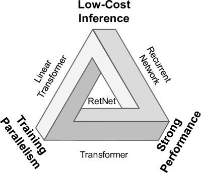
Numerous efforts have continued to develop the next-generation architecture, aiming at retaining training parallelism and competitive performance as Transformers while having efficient $O(1)$ inference. It is challenging to achieve the above goals simultaneously, i.e., the so-called “impossible triangle” as shown in Figure 2.

There have been three main strands of research. First, linearized attention [19] approximates standard attention scores $\exp({\bm{q}}\cdot{\bm{k}})$ with kernels $\phi({\bm{q}})\cdot\phi({\bm{k}})$, so that autoregressive inference can be rewritten in a recurrent form. However, the modeling capability and performance are worse than Transformers, which hinders the method’s popularity. The second strand returns to recurrent models for efficient inference while sacrificing training parallelism. As a remedy, element-wise operators [25] are used for acceleration, however, representation capacity and performance are harmed. The third line of research explores replacing attention with other mechanisms, such as S4 [11], and its variants [8, 26]. None of the previous work can break through the impossible triangle, resulting in no clear winner compared with Transformers.

In this work, we propose retentive networks (RetNet), achieving low-cost inference, efficient long-sequence modeling, Transformer-comparable performance, and parallel model training simultaneously. Specifically, we introduce a multi-scale retention mechanism to substitute multi-head attention, which has three computation paradigms, i.e., parallel, recurrent, and chunkwise recurrent representations. First, the parallel representation empowers training parallelism to utilize GPU devices fully. Second, the recurrent representation enables efficient $O(1)$ inference in terms of memory and computation. The deployment cost and latency can be significantly reduced. Moreover, the implementation is greatly simplified without key-value cache tricks. Third, the chunkwise recurrent representation can perform efficient long-sequence modeling. We parallelly encode each local block for computation speed while recurrently encoding the global blocks to save GPU memory.

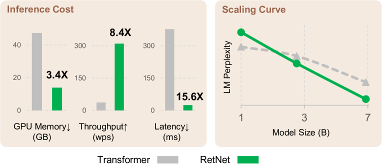
We conduct extensive experiments to compare RetNet with Transformer and its variants. Experimental results on language modeling show that RetNet is consistently competitive in terms of both scaling curves and in-context learning. Moreover, the inference cost of RetNet is length-invariant. For a 7B model and 8k sequence length, RetNet decodes 8.4$\times$ faster and saves 70% of memory than Transformers with key-value caches. During training, RetNet also achieves 25-50% memory saving and 7$\times$ acceleration than standard Transformer and an advantage towards highly-optimized FlashAttention [7]. Besides, RetNet’s inference latency is insensitive to batch size, allowing enormous throughput. The intriguing properties make RetNet a strong successor to Transformer for large language models.

2 Retentive Networks

Retentive network (RetNet) is stacked with $L$ identical blocks, which follows a similar layout (i.e., residual connection, and pre-LayerNorm) as in Transformer [34]. Each RetNet block contains two modules: a multi-scale retention (MSR) module, and a feed-forward network (FFN) module. We introduce the MSR module in the following sections. Given an input sequence $x=x_{1}\cdots x_{|x|}$, RetNet encodes the sequence in an autoregressive way. The input vectors $\{{\bm{x}}_{i}\}_{i=1}^{|x|}$ is first packed into $X^{0}=[{\bm{x}}_{1},\cdots,{\bm{x}}_{|x|}]\in\mathbb{R}^{|x|\times d_{\text{model}}}$, where $d_{\text{model}}$ is hidden dimension. Then we compute contextualized vector representations $X^{l}=\mathrm{RetNet}_{l}(X^{l-1}),l\in[1,L]$.

2.1 Retention

In this section, we introduce the retention mechanism that has a dual form of recurrence and parallelism. So we can train the models in a parallel way while recurrently conducting inference.

Given input $X\in\mathbb{R}^{|x|\times d_{\text{model}}}$, we project it to one-dimensional function $v(n)=X_{n}\cdot{\bm{w}}_{V}$. Consider a sequence modeling problem that maps $v(n)\mapsto o(n)$ through states ${\bm{s}}_{n}$. Let $v_{n},o_{n}$ denote $v(n),o(n)$ for simplicity. We formulate the mapping in a recurrent manner:

$${\bm{s}}_{n}=A{\bm{s}}_{n-1}+K_{n}^{\intercal}v_{n}, A\in\mathbb{R}^{d\times d},K_{n}\in\mathbb{R}^{1\times d}$$ (1)

$$o_{n}=Q_{n}{\bm{s}}_{n}=\sum_{m=1}^{n}Q_{n}A^{n-m}K_{m}^{\intercal}v_{m}, Q_{n}\in\mathbb{R}^{1\times d}$$

where we map $v_{n}$ to the state vector ${\bm{s}}_{n}$, and then implement a linear transform to encode sequence information recurrently.

Next, we make the projection $Q_{n},K_{n}$ content-aware:

$$Q=XW_{Q},\quad K=XW_{K}$$ (2)

where $W_{Q},W_{K}\in\mathbb{R}^{d\times d}$ are learnable matrices.

We diagonalize the matrix $A=\Lambda(\gamma e^{i\theta})\Lambda^{-1}$, where $\gamma,\theta\in\mathbb{R}^{d}$. Then we obtain $A^{n-m}=\Lambda(\gamma e^{i\theta})^{n-m}\Lambda^{-1}$. By absorbing $\Lambda$ into $W_{Q}$ and $W_{K}$, we can rewrite Equation (LABEL:eq:rnn) as:

$$o_{n} =\sum_{m=1}^{n}Q_{n}(\gamma e^{i\theta})^{n-m}K_{m}^{\intercal}v_{m}$$ (3)

$$=\sum_{m=1}^{n}(Q_{n}(\gamma e^{i\theta})^{n})(K_{m}(\gamma e^{i\theta})^{-m})^{\intercal}v_{m}$$

where $Q_{n}(\gamma e^{i\theta})^{n},K_{m}(\gamma e^{i\theta})^{-m}$ is known as xPos [29], i.e., a relative position embedding proposed for Transformer. We further simplify $\gamma$ as a scalar, Equation (3) becomes:

$$o_{n}=\sum_{m=1}^{n}\gamma^{n-m}(Q_{n}e^{in\theta})(K_{m}e^{im\theta})^{\dagger}v_{m}$$ (4)

where ^† is the conjugate transpose. The formulation is easily parallelizable within training instances.

In summary, we start with recurrent modeling as shown in Equation (LABEL:eq:rnn), and then derive its parallel formulation in Equation (4). We consider the original mapping $v(n)\mapsto o(n)$ as vectors and obtain the retention mechanism as follows.

(a) Parallel representation.

(b) Recurrent representation.

Figure 3: Dual form of RetNet. “GN” is short for GroupNorm.

The Parallel Representation of Retention

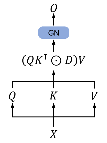
As shown in Figure 3(a), the retention layer is defined as:

$$Q=(XW_{Q})\odot\Theta, \quad K=(XW_{K})\odot\overline{\Theta},\quad V=XW_{V}$$ (5)

$$\Theta_{n}=e^{in\theta}, \quad D_{nm}=\left\{\begin{aligned} &\gamma^{n-m},&n\geq m\\ &0,&n<m\\ \end{aligned}\right.$$

$$\mathrm{Rete} \mathrm{ntion}(X)=(QK^{\intercal}\odot D)V$$

where $\overline{\Theta}$ is the complex conjugate of $\Theta$, and $D\in\mathbb{R}^{|x|\times|x|}$ combines causal masking and exponential decay along relative distance as one matrix. Similar to self-attention, the parallel representation enables us to train the models with GPUs efficiently.

The Recurrent Representation of Retention

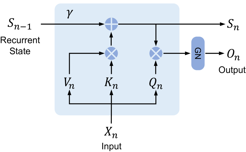
As shown in Figure 3(b), the proposed mechanism can also be written as recurrent neural networks (RNNs), which is favorable for inference. For the $n$-th timestep, we recurrently obtain the output as:

$$S_{n}=\gamma S_{n-1}+K_{n}^{\intercal}V_{n}$$ (6)

$$\mathrm{Rete}\mathrm{ntion}(X_{n})=Q_{n}S_{n},\quad n=1,\cdots,|x|$$

where $Q,K,V,\gamma$ are the same as in Equation (5).

The Chunkwise Recurrent Representation of Retention

A hybrid form of parallel representation and recurrent representation is available to accelerate training, especially for long sequences. We divide the input sequences into chunks. Within each chunk, we follow the parallel representation (Equation (5)) to conduct computation. In contrast, cross-chunk information is passed following the recurrent representation (Equation (LABEL:eq:ret:recurrent)). Specifically, let $B$ denote the chunk length. We compute the retention output of the $i$-th chunk via:

$$Q_{[i]}=Q_{Bi:B(i+1)} ,\quad K_{[i]}=K_{Bi:B(i+1)},\quad V_{[i]}=V_{Bi:B(i+1)}$$ (7)

$$R_{i} =K_{[i]}^{\intercal}(V_{[i]}\odot\zeta)+\gamma^{B}R_{i-1},\quad\zeta_{ij}=\gamma^{B-i-1}$$

$$\mathrm{Rete}\mathrm{ntion}(X_{[i]}) =\underbrace{(Q_{[i]}K^{\intercal}_{[i]}\odot D)V_{[i]}}_{\text{Inner-Chunk}}+\underbrace{(Q_{[i]}R_{i-1})\odot\xi}_{\text{Cross-Chunk}},\quad\xi_{ij}=\gamma^{i+1}$$

where ${[i]}$ indicates the $i$-th chunk, i.e., $x_{[i]}=[x_{(i-1)B+1},\cdots,x_{iB}]$.

2.2 Gated Multi-Scale Retention

We use $h=\nicefrac{{d_{\text{model}}}}{{d}}$ retention heads in each layer, where $d$ is the head dimension. The heads use different parameter matrices $W_{Q},W_{K},W_{V}\in\mathbb{R}^{d\times d}$. Moreover, multi-scale retention (MSR) assigns different $\gamma$ for each head. For simplicity, we set $\gamma$ identical among different layers and keep them fixed. In addition, we add a $\mathrm{swish}$ gate [14, 28] to increase the non-linearity of retention layers. Formally, given input $X$, we define the layer as:

$$\mathbf{\gamma} =1-2^{-5-\mathrm{arange}(0,h)}\in\mathbb{R}^{h}$$ (8)

$$\mathrm{head}_{i} =\mathrm{Retention}(X,\gamma_{i})$$

$$Y =\mathrm{GroupNorm}_{h}(\mathrm{Concat}(\mathrm{head}_{1},\cdots,\mathrm{head}_{h}))$$

$$\mathrm{MSR}(X) =(\mathrm{swish}(XW_{G})\odot Y)W_{O}$$

where $W_{G},W_{O}\in\mathbb{R}^{d_{\text{model}}\times d_{\text{model}}}$ are learnable parameters, and $\mathrm{GroupNorm}$ [35] normalizes the output of each head, following SubLN proposed in [32]. Notice that the heads use multiple $\gamma$ scales, which results in different variance statistics. So we normalize the head outputs separately.

⬇

def ParallelRetention(

q, # bsz * num_head * len * qk_dim

k, # bsz * num_head * len * qk_dim

v, # bsz * num_head * len * v_dim

decay_mask # num_head * len * len

):

retention = q @ k.transpose(-1, -2)

retention = retention * decay_mask

output = retention @ v

output = group_norm(output)

return output

⬇

def RecurrentRetention(

q, k, v, # bsz * num_head * len * qkv_dim

past_kv, # bsz * num_head * qk_dim * v_dim

decay # num_head * 1 * 1

):

current_kv = decay * past_kv + k.unsqueeze(-1) * v.unsqueeze(-2)

output = torch.sum(q.unsqueeze(-1) * current_kv, dim=-2)

output = group_norm(output)

return output, current_kv

⬇

def ChunkwiseRetention(

q, k, v, # bsz * num_head * chunk_size * qkv_dim

past_kv, # bsz * num_head * qk_dim * v_dim

decay_mask, # num_head * chunk_size * chunk_size

chunk_decay, # num_head * 1 * 1

inner_decay, # num_head * chunk_size

):

retention = q @ k.transpose(-1, -2)

retention = retention * decay_mask

inner_retention = retention @ v

cross_retention = (q @ past_kv) * inner_decay

retention = inner_retention + cross_retention

output = group_norm(retention)

current_kv = chunk_decay * past_kv + k.transpose(-1, -2) @ v

return output, current_kv

Figure 4: Pseudocode for the three computation paradigms of retention.

The pseudocode of retention is summarized in Figure 4.

Retention Score Normalization

We utilize the scale-invariant nature of $\mathrm{GroupNorm}$ to improve the numerical precision of retention layers. Specifically, multiplying a scalar value within $\mathrm{GroupNorm}$ does not affect outputs and backward gradients, i.e., $\mathrm{GroupNorm}(\alpha*\mathrm{head}_{i})=\mathrm{GroupNorm}(\mathrm{head}_{i})$. We implement three normalization factors in Equation (5). First, we normalize $QK^{\intercal}$ as $\nicefrac{{QK^{\intercal}}}{{\sqrt{d}}}$. Second, we replace $D$ with $\tilde{D}_{nm}=\nicefrac{{D_{nm}}}{{\sqrt{\sum_{i=1}^{n}D_{ni}}}}$. Third, let $R$ denote the retention scores $R=QK^{\intercal}\odot D$, we normalize it as $\tilde{R}_{nm}=\nicefrac{{R_{nm}}}{{\max(|\sum_{i=1}^{n}R_{ni}|,1)}}$. Then the retention output becomes $\mathrm{Retention}(X)=\tilde{R}V$. The above tricks do not affect the final results while stabilizing the numerical flow of both forward and backward passes, because of the scale-invariant property.

2.3 Overall Architecture of Retention Networks

For an $L$-layer retention network, we stack multi-scale retention (MSR) and feed-forward network (FFN) to build the model. Formally, the input sequence $\{x_{i}\}_{i=1}^{|x|}$ is transformed to vectors by a word embedding layer. We use the packed embeddings $X^{0}=[{\bm{x}}_{1},\cdots,{\bm{x}}_{|x|}]\in\mathbb{R}^{|x|\times d_{\text{model}}}$ as the input and compute the model output $X^{L}$:

$$Y^{l} =\mathrm{MSR}(\mathrm{LN}(X^{l}))+X^{l}$$ (9)

$$X^{l+1} =\mathrm{FFN}(\mathrm{LN}(Y^{l}))+Y^{l}$$

where $\mathrm{LN}(\cdot)$ is LayerNorm [1]. The FFN part is computed as $\mathrm{FFN}(X)=\mathrm{gelu}(XW_{1})W_{2}$, where $W_{1},W_{2}$ are parameter matrices.

Training

We use the parallel (Equation (5)) and chunkwise recurrent (Equation (7)) representations during the training process. The parallelization within sequences or chunks efficiently utilizes GPUs to accelerate computation. More favorably, chunkwise recurrence is especially useful for long-sequence training, which is efficient in terms of both FLOPs and memory consumption.

Inference

The recurrent representation (Equation (LABEL:eq:ret:recurrent)) is employed during the inference, which nicely fits autoregressive decoding. The $O(1)$ complexity reduces memory and inference latency while achieving equivalent results.

2.4 Relation to and Differences from Previous Methods

Table 1 compares RetNet with previous methods from various perspectives. The comparison results echo the “impossible triangle” presented in Figure 2. Moreover, RetNet has linear memory complexity for long sequences due to the chunkwise recurrent representation. We also summarize the comparisons with specific methods as follows.

Transformer

The parallel representation of retention shares similar spirits as Transformers [34]. The most related Transformer variant is Lex Transformer [29] which implements xPos as position embeddings. As described in Equation (3), the derivation of retention aligns with xPos. In comparison with attention, retention removes $\mathrm{softmax}$ and enables recurrent formulation, which significantly benefits inference.

S4

Unlike Equation (2), if $Q_{n}$ and $K_{n}$ are content-unaware, the formulation can be degenerated to S4 [11], where $O=(QK^{\intercal},QAK^{\intercal},..,QA^{|x|-1}K^{\intercal})*V$.

Linear Attention

The variants typically use various kernels $\nicefrac{{\phi(q_{i})\phi(k_{j})}}{{\sum_{n=1}^{|x|}\phi(q_{i})\phi(k_{n})}}$ to replace the $\mathrm{softmax}$ function. However, linear attention struggles to effectively encode position information, rendering the models less performant. Besides, we reexamine sequence modeling from scratch, rather than aiming at approximating $\mathrm{softmax}$.

AFT/RWKV

Attention Free Transformer (AFT) simplifies dot-product attention to element-wise operations and moves $\mathrm{softmax}$ to key vectors. RWKV replaces AFT’s position embeddings with exponential decay and runs the models recurrently for training and inference. In comparison, retention preserves high-dimensional states to encode sequence information, which contributes to expressive ability and better performance.

xPos/RoPE

Compared with relative position embedding methods proposed for Transformers, Equation 3 presents a similar formulation as xPos [29] and RoPE [31].

Sub-LayerNorm

As shown in Equation (8), the retention layer uses Sub-LayerNorm [37] to normalize outputs. Because the multi-scale modeling leads to different variances for the heads, we replace the original LayerNorm with GroupNorm.

Architectures	Training Parallelization	Inference Cost	Long-Sequence Memory Complexity	Performance
Transformer	✔	$O(N)$	$O(N^{2})$	✔✔
Linear Transformer	✔	$O(1)$	$O(N)$	✘
Recurrent NN	✘	$O(1)$	$O(N)$	✘
RWKV	✘	$O(1)$	$O(N)$	✔
H3/S4	✔	$O(1)$	$O(N\log N)$	✔
Hyena	✔	$O(N)$	$O(N\log N)$	✔
RetNet	✔	$O(1)$	$O(N)$	✔✔

Table 1: Model comparison from various perspectives. RetNet achieves training parallelization, constant inference cost, linear long-sequence memory complexity, and good performance.

3 Experiments

We conduct experiments on language modeling to evaluate RetNet. We evaluate the proposed architecture with various benchmarks, i.e., language modeling performance, and zero-/few-shot learning on downstream tasks. Moreover, for training and inference, we compare speed, memory consumption, and latency.

3.1 Setup

Parameter Allocation

We re-allocate the parameters in MSR and FFN for fair comparisons. Let $d$ denote $d_{\text{model}}$ for simplicity here. In Transformers, there are about $4d^{2}$ parameters in self-attention where $W_{Q},W_{K},W_{V},W_{O}\in\mathbb{R}^{d\times d}$, and $8d^{2}$ parameters in FFN where the intermediate dimension is $4d$. In comparison, RetNet has $8d^{2}$ parameters in retention, where $W_{Q},W_{K}\in\mathbb{R}^{d\times d},W_{G},W_{V}\in\mathbb{R}^{d\times 2d},W_{O}\in\mathbb{R}^{2d\times d}$. Notice that the head dimension of $V$ is twice $Q,K$. The widened dimension is projected back to $d$ by $W_{O}$. In order to keep the parameter number the same as Transformer, the FFN intermediate dimension in RetNet is $2d$. Meanwhile, we set the head dimension to $256$ in our experiments, i.e., $256$ for queries and keys, and $512$ for values. For fair comparison, we keep $\mathbf{\gamma}$ identical among different model sizes, where $\mathbf{\gamma}=1-e^{\mathrm{linspace}(\log\nicefrac{{1}}{{32}},\log\nicefrac{{1}}{{512}},h)}\in\mathbb{R}^{h}$ instead of the default value in Equation (8).

Size	Hidden Dim.	#Layers	Batch Size	# Tokens	Learning Rate
1.3B	2048	24	4M	100B	$6\times 10^{-4}$
2.7B	2560	32	4M	100B	$3\times 10^{-4}$
6.7B	4096	32	4M	100B	$3\times 10^{-4}$

Table 2: Sizes, and learning hyper-parameters of the models in language modeling experiments.

Language Model Training

As shown in Table 2, we train language models with various sizes (i.e., 1.3B, 2.7B, and 6.7B) from scratch. The training corpus is a curated compilation of The Pile [10], C4 [9], and The Stack [18]. We append the <bos> token to indicate the start of a sequence. The training batch size is 4M tokens with 2048 maximal length. We train the models with 100B tokens, i.e., 25k steps. We use the AdamW [21] optimizer with $\beta_{1}=0.9,\beta_{2}=0.98$, and weight decay is set to $0.05$. The number of warmup steps is 375 with linear learning rate decay. The parameters are initialized following DeepNet [36] to guarantee training stability. The implementation is based on TorchScale [23]. We train the models with 512 AMD MI200 GPUs.

3.2 Comparisons with Transformer

Figure 5: Perplexity decreases along with scaling up the model size. We empirically observe that RetNet tends to outperform Transformer when the model size is larger than 2B.

Language Modeling

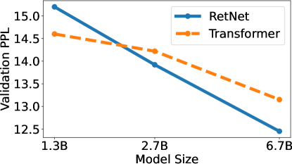
As shown in Figure 5, we report perplexity on the validation set for the language models based on Transformer and RetNet. We present the scaling curves with three model sizes, i.e., 1.3B, 2.7B, and 6.7B. RetNet achieves comparable results with Transformers. More importantly, the results indicate that RetNet is favorable regarding size scaling. Besides performance, the RetNet training is quite stable in our experiments. Experimental results show that RetNet is a strong competitor to Transformer for large language models. Empirically, we find that RetNet starts to outperform Transformer when the model size is larger than 2B. We also summarize the language modeling results with different context lengths in Appendix B.

	HS	BoolQ	COPA	PIQA	Winograd	Winogrande	SC	Avg
Zero-Shot
Transformer	55.9	62.0	69.0	74.6	69.5	56.5	75.0	66.07
RetNet	60.7	62.2	77.0	75.4	77.2	58.1	76.0	69.51
4-Shot
Transformer	55.8	58.7	71.0	75.0	71.9	57.3	75.4	66.44
RetNet	60.5	60.1	78.0	76.0	77.9	59.9	75.9	69.76

Table 3: Zero-shot and few-shot learning with Transformer and RetNet. The model size is 6.7B.

Zero-Shot and Few-Shot Evaluation on Downstream Tasks

We also compare the language models on a wide range of downstream tasks. We evaluate zero-shot and 4-shot learning with the 6.7B models. As shown in Table 3, the datasets include HellaSwag (HS) [39], BoolQ [6], COPA [38], PIQA [3], Winograd, Winogrande [20], and StoryCloze (SC) [22]. The accuracy numbers are consistent with language modeling perplexity presented in Figure 5. RetNet achieves comparable performance with Transformer on zero-shot and in-context learning settings.

3.3 Training Cost

Model Size	Memory (GB) $\downarrow$			Throughput (wps) $\uparrow$
	Trm	Trm+FlashAttn	RetNet	Trm	Trm+FlashAttn	RetNet
1.3B	74.8	38.8	34.5	10832.4	63965.2	73344.8
2.7B	69.6	42.1	42.0	5186.0	34990.2	38921.2
6.7B	69.0	51.4	48.0	2754.4	16230.1	17458.6
13B	61.4	46.3	45.9	1208.9	7945.1	8642.2

Table 4: Training cost of Transformer (Trm), Transformer with FlashAttention (Trm+FlashAttn), and RetNet. We report memory consumption and training throughput (word per second; wps).

As shown in Table 4, we compare the training speed and memory consumption of Transformer and RetNet, where the training sequence length is 8192. We also compare with FlashAttention [7], which improves speed and reduces GPU memory IO by recomputation and kernel fusion. In comparison, we implement RetNet using vanilla PyTorch code, and leave kernel fusion or FlashAttention-like acceleration for future work. We use chunkwise recurrent representation of retention as described in Equation (7). The chunk size is set to $512$. We evaluate the results with eight Nvidia A100-80GB GPUs, because FlashAttention is highly optimized for A100. Tensor parallelism is enabled for 6.7B and 13B models.

Experimental results show that RetNet is more memory-efficient and has higher throughput than Transformers during training. Even compared with FlashAttention, RetNet is still competitive in terms of speed and memory cost. Moreover, without relying on specific kernels, it is easy to train RetNet on other platforms efficiently. For example, we train the RetNet models on an AMD MI200 cluster with decent throughput. It is notable that RetNet has the potential to further reduce cost via advanced implementation, such as kernel fusion.

3.4 Inference Cost

(a) GPU memory cost of Transformer and RetNet.

(b) Throughput of Transformer and RetNet.

(c) Inference latency with different batch sizes.

Figure 6: Inference cost of Transformer and RetNet with a model size of 6.7B. RetNet outperforms Transformers in terms of memory consumption, throughput, and latency.

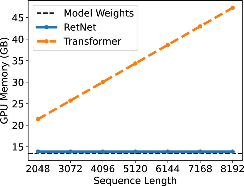
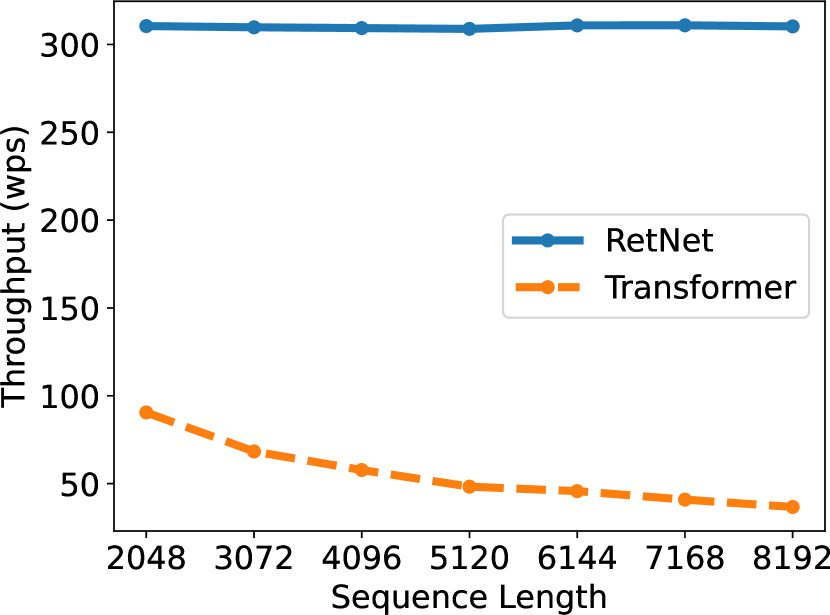
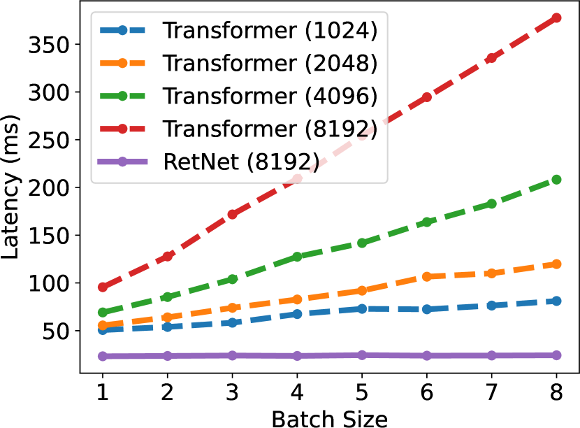
As shown in Figure 6, we compare memory cost, throughput, and latency of Transformer and RetNet during inference. Transformers reuse KV caches of previously decoded tokens. RetNet uses the recurrent representation as described in Equation (LABEL:eq:ret:recurrent). We evaluate the 6.7B model on the A100-80GB GPU in our experiments. Figure 6 shows that RetNet outperforms Transformer in terms of inference cost.

Memory

As shown in Figure 6(a), the memory cost of Transformer increases linearly due to KV caches. In contrast, the memory consumption of RetNet remains consistent even for long sequences, requiring much less GPU memory to host RetNet. The additional memory consumption of RetNet is almost negligible (i.e., about 3%) while the model weights occupy 97%.

Throughput

As presented in Figure 6(b), the throughput of Transformer drops along with the decoding length increases. In comparison, RetNet has higher and length-invariant throughput during decoding, by utilizing the recurrent representation of retention.

Latency

Latency is an important metric in deployment, which greatly affects user experience. We report decoding latency in Figure 6(c). Experimental results show that increasing batch size renders Transformer’s latency larger. Moreover, the latency of Transformers grows faster with longer input. In order to make latency acceptable, we have to restrict the batch size, which harms the overall inference throughput of Transformers. By contrast, RetNet’s decoding latency outperforms Transformers and keeps almost the same across different batch sizes and input lengths.

3.5 Comparison with Transformer Variants

Method	In-Domain	PG22	QMSum	GovReport	SummScreen
RWKV	30.92	51.41	28.17	19.80	25.78
H3	29.97	49.17	24.29	19.19	25.11
Hyena	32.08	52.75	28.18	20.55	26.51
Linear Transformer	40.24	63.86	28.45	25.33	32.02
RetNet	26.05	45.27	21.33	16.52	22.48

Table 5: Perplexity results on language modeling. RetNet outperforms other architectures on both the in-domain evaluation set and various out-of-domain corpora.

Apart from Transformer, we compare RetNet with various efficient Transformer variants, including Linear Transformer [19], RWKV [25], H3 [8], and Hyena [26]. All models have 200M parameters with 16 layers and a hidden dimension of 1024. For H3, we set the head dimension as 8. For RWKV, we use the TimeMix module to substitute self-attention layers while keeping FFN layers consistent with other models for fair comparisons. We train the models with 10k steps with a batch size of 0.5M tokens. Most hyperparameters and training corpora are kept the same as in Section 3.1.

Table 5 reports the perplexity numbers on the in-domain validation set and other out-of-domain corpora, e.g., Project Gutenberg 2019-2022 (PG22) [29], QMSum [40], GovReport [12], SummScreen [4, 33]. Overall, RetNet outperforms previous methods across different datasets. RetNet not only achieves better evaluation results on the in-domain corpus but also obtains lower perplexity on several out-of-domain datasets. The favorable performance makes RetNet a strong successor to Transformer, besides the benefits of significant cost reduction (Sections 3.3 and 3.4).

In addition, we discuss the training and inference efficiency of the compared methods. Let $d$ denote the hidden dimension, and $n$ the sequence length. For training, RWKV’s token-mixing complexity is $O(dn)$ while Hyena’s is $O(dn\log n)$ with Fast Fourier Transform acceleration. The above two methods reduce training FLOPS via employing element-wise operators to trade-off modeling capacity. In comparison with retention, the chunk-wise recurrent representation is $O(dn(b+h))$, where $b$ is the chunk size, $h$ is the head dimension, and we usually set $b=512,h=256$. For either large model size (i.e., larger $d$) or sequence length, the additional $b+h$ has negligible effects. So the RetNet training is quite efficient without sacrificing the modeling performance. For inference, among the compared efficient architectures, Hyena has the same complexity (i.e., $O(n)$ per step) as Transformer while the others can perform $O(1)$ decoding.

3.6 Ablation Studies

Method	In-Domain	PG22	QMSum	GovReport	SummScreen
RetNet	26.05	45.27	21.33	16.52	22.48
$-$ $\mathrm{swish}$ gate	27.84	49.44	22.52	17.45	23.72
$-$ $\mathrm{GroupNorm}$	27.54	46.95	22.61	17.59	23.73
$-$ $\gamma$ decay	27.86	47.85	21.99	17.49	23.70
$-$ multi-scale decay	27.02	47.18	22.08	17.17	23.38
Reduce head dimension	27.68	47.72	23.09	17.46	23.41

Table 6: Ablation results on in-domain and out-of-domain corpora.

We ablate various design choices of RetNet and report the language modeling results in Table 6. The evaluation settings and metrics are the same as in Section 3.5.

Architecture

We ablate the $\mathrm{swish}$ gate and $\mathrm{GroupNorm}$ as described in Equation 8. Table 6 shows that the above two components improve the final performance. Firstly, the gating module is essential for enhancing non-linearity and improving model capability. Notice that we use the same parameter allocation as Transformers after removing the gate. Secondly, group normalization in retention balances the variances of multi-head outputs, which improves training stability and language modeling results.

Multi-Scale Decay

Equation 8 shows that we use different $\mathbf{\gamma}$ as the decay rates for the retention heads. In the ablation studies, we examine removing $\gamma$ decay (i.e., “$-$ $\gamma$ decay”) and applying the same decay rate across heads (i.e., “$-$ multi-scale decay”). Specifically, ablating $\gamma$ decay is equivalent to $\gamma=1$. In the second setting, we set $\gamma=127/128$ for all heads. Table 6 indicates that both the decay mechanism and using multiple decay rates can improve the language modeling performance.

Head Dimension

From the recurrent perspective of LABEL:eq:rnn, the head dimension implies the memory capacity of hidden states. In the ablation study, we reduce the default head dimension from $256$ to $64$, i.e., $64$ for queries and keys, and $128$ for values. We keep the hidden dimension $d_{\text{model}}$ the same so the number of heads increases. Experimental results in Table 6 show that the larger head dimension achieves better performance.

4 Conclusion

In this work, we propose retentive networks (RetNet) for sequence modeling, which enables various representations, i.e., parallel, recurrent, and chunkwise recurrent. RetNet achieves significantly better inference efficiency (in terms of memory, speed, and latency), favorable training parallelization, and competitive performance compared with Transformers. The above advantages make RetNet an ideal successor to Transformers for large language models, especially considering the deployment benefits brought by the $O(1)$ inference complexity. In the future, we would like to scale up RetNet in terms of model size [5] and training steps. Moreover, retention can efficiently work with structured prompting [17] by compressing long-term memory. We will also use RetNet as the backbone architecture to train multimodal large language models [16, 13, 27]. In addition, we are interested in deploying RetNet models on various edge devices, such as mobile phones.

Appendix A Hyperparameters

Hyperparameters	1.3B	2.7B	6.7B
Layers	24	32	32
Hidden size	2048	2560	4096
FFN size	4096	5120	8192
Heads	8	10	16
Learning rate	$6\times 10^{-4}$	$3\times 10^{-4}$	$3\times 10^{-4}$
LR scheduler	Polynomial decay
Warm-up steps	375
Tokens per batch	4M
Adam $\beta$	(0.9, 0.98)
Training steps	25,000
Gradient clipping	2.0
Dropout	0.1
Weight decay	0.01

Table 7: Hyperparamters used for the models in Section 3.

Appendix B Grouped Results of Different Context Lengths

As shown in Table 8, we report language modeling results with different context lengths. In order to make the numbers comparable, we use 2048 text chunks as evaluation data and only compute perplexity for the last 128 tokens. Experimental results show that RetNet outperforms Transformer across different context lengths. Besides, RetNet can utilize longer context for better results.

Model	512	1024	2048
Transformer	13.55	12.56	12.35
RetNet	13.09	12.14	11.98

Table 8: Language modeling perplexity of RetNet and Transformer with different context length. The results show that RetNet has a consistent advantage across sequence length.

References

- BKH [16] Jimmy Lei Ba, Jamie Ryan Kiros, and Geoffrey E Hinton. Layer normalization. arXiv preprint arXiv:1607.06450, 2016.
- BMR+ [20] Tom Brown, Benjamin Mann, Nick Ryder, Melanie Subbiah, Jared D Kaplan, Prafulla Dhariwal, Arvind Neelakantan, Pranav Shyam, Girish Sastry, Amanda Askell, Sandhini Agarwal, Ariel Herbert-Voss, Gretchen Krueger, Tom Henighan, Rewon Child, Aditya Ramesh, Daniel Ziegler, Jeffrey Wu, Clemens Winter, Chris Hesse, Mark Chen, Eric Sigler, Mateusz Litwin, Scott Gray, Benjamin Chess, Jack Clark, Christopher Berner, Sam McCandlish, Alec Radford, Ilya Sutskever, and Dario Amodei. Language models are few-shot learners. In Advances in Neural Information Processing Systems, volume 33, pages 1877–1901. Curran Associates, Inc., 2020.
- BZB+ [20] Yonatan Bisk, Rowan Zellers, Ronan Le Bras, Jianfeng Gao, and Yejin Choi. Piqa: Reasoning about physical commonsense in natural language. In Thirty-Fourth AAAI Conference on Artificial Intelligence, 2020.
- CCWG [21] Mingda Chen, Zewei Chu, Sam Wiseman, and Kevin Gimpel. Summscreen: A dataset for abstractive screenplay summarization. arXiv preprint arXiv:2104.07091, 2021.
- CDH+ [22] Zewen Chi, Li Dong, Shaohan Huang, Damai Dai, Shuming Ma, Barun Patra, Saksham Singhal, Payal Bajaj, Xia Song, Xian-Ling Mao, Heyan Huang, and Furu Wei. On the representation collapse of sparse mixture of experts. In Advances in Neural Information Processing Systems, 2022.
- CLC+ [19] Christopher Clark, Kenton Lee, Ming-Wei Chang, Tom Kwiatkowski, Michael Collins, and Kristina Toutanova. BoolQ: Exploring the surprising difficulty of natural yes/no questions. In Proceedings of the 2019 Conference of the North American Chapter of the Association for Computational Linguistics, pages 2924–2936, 2019.
- DFE+ [22] Tri Dao, Dan Fu, Stefano Ermon, Atri Rudra, and Christopher Ré. Flashattention: Fast and memory-efficient exact attention with io-awareness. Advances in Neural Information Processing Systems, 35:16344–16359, 2022.
- DFS+ [22] Tri Dao, Daniel Y Fu, Khaled K Saab, Armin W Thomas, Atri Rudra, and Christopher Ré. Hungry hungry hippos: Towards language modeling with state space models. arXiv preprint arXiv:2212.14052, 2022.
- DMI+ [21] Jesse Dodge, Ana Marasović, Gabriel Ilharco, Dirk Groeneveld, Margaret Mitchell, and Matt Gardner. Documenting large webtext corpora: A case study on the colossal clean crawled corpus. In Conference on Empirical Methods in Natural Language Processing, 2021.
- GBB+ [20] Leo Gao, Stella Biderman, Sid Black, Laurence Golding, Travis Hoppe, Charles Foster, Jason Phang, Horace He, Anish Thite, Noa Nabeshima, et al. The Pile: An 800GB dataset of diverse text for language modeling. arXiv preprint arXiv:2101.00027, 2020.
- GGR [21] Albert Gu, Karan Goel, and Christopher Ré. Efficiently modeling long sequences with structured state spaces. arXiv preprint arXiv:2111.00396, 2021.
- HCP+ [21] Luyang Huang, Shuyang Cao, Nikolaus Parulian, Heng Ji, and Lu Wang. Efficient attentions for long document summarization. arXiv preprint arXiv:2104.02112, 2021.
- HDW+ [23] Shaohan Huang, Li Dong, Wenhui Wang, Yaru Hao, Saksham Singhal, Shuming Ma, Tengchao Lv, Lei Cui, Owais Khan Mohammed, Qiang Liu, Kriti Aggarwal, Zewen Chi, Johan Bjorck, Vishrav Chaudhary, Subhojit Som, Xia Song, and Furu Wei. Language is not all you need: Aligning perception with language models. ArXiv, abs/2302.14045, 2023.
- HG [16] Dan Hendrycks and Kevin Gimpel. Gaussian error linear units (GELUs). arXiv: Learning, 2016.
- HS [97] Sepp Hochreiter and Jürgen Schmidhuber. Long short-term memory. Neural Computation, 9:1735–1780, November 1997.
- [16] Yaru Hao, Haoyu Song, Li Dong, Shaohan Huang, Zewen Chi, Wenhui Wang, Shuming Ma, and Furu Wei. Language models are general-purpose interfaces. ArXiv, abs/2206.06336, 2022.
- [17] Yaru Hao, Yutao Sun, Li Dong, Zhixiong Han, Yuxian Gu, and Furu Wei. Structured prompting: Scaling in-context learning to 1,000 examples. ArXiv, abs/2212.06713, 2022.
- KLBA+ [22] Denis Kocetkov, Raymond Li, Loubna Ben Allal, Jia Li, Chenghao Mou, Carlos Muñoz Ferrandis, Yacine Jernite, Margaret Mitchell, Sean Hughes, Thomas Wolf, Dzmitry Bahdanau, Leandro von Werra, and Harm de Vries. The Stack: 3TB of permissively licensed source code. Preprint, 2022.
- KVPF [20] Angelos Katharopoulos, Apoorv Vyas, Nikolaos Pappas, and François Fleuret. Transformers are rnns: Fast autoregressive transformers with linear attention. In International Conference on Machine Learning, pages 5156–5165. PMLR, 2020.
- LDM [12] Hector Levesque, Ernest Davis, and Leora Morgenstern. The winograd schema challenge. In Thirteenth International Conference on the Principles of Knowledge Representation and Reasoning, 2012.
- LH [19] Ilya Loshchilov and Frank Hutter. Decoupled weight decay regularization. In International Conference on Learning Representations, 2019.
- MRL+ [17] Nasrin Mostafazadeh, Michael Roth, Annie Louis, Nathanael Chambers, and James Allen. Lsdsem 2017 shared task: The story cloze test. In Proceedings of the 2nd Workshop on Linking Models of Lexical, Sentential and Discourse-level Semantics, pages 46–51, 2017.
- MWH+ [22] Shuming Ma, Hongyu Wang, Shaohan Huang, Wenhui Wang, Zewen Chi, Li Dong, Alon Benhaim, Barun Patra, Vishrav Chaudhary, Xia Song, and Furu Wei. TorchScale: Transformers at scale. CoRR, abs/2211.13184, 2022.
- OSG+ [23] Antonio Orvieto, Samuel L. Smith, Albert Gu, Anushan Fernando, Caglar Gulcehre, Razvan Pascanu, and Soham De. Resurrecting recurrent neural networks for long sequences. ArXiv, abs/2303.06349, 2023.
- PAA+ [23] Bo Peng, Eric Alcaide, Quentin Anthony, Alon Albalak, Samuel Arcadinho, Huanqi Cao, Xin Cheng, Michael Chung, Matteo Grella, Kranthi Kiran GV, Xuzheng He, Haowen Hou, Przemyslaw Kazienko, Jan Kocon, Jiaming Kong, Bartlomiej Koptyra, Hayden Lau, Krishna Sri Ipsit Mantri, Ferdinand Mom, Atsushi Saito, Xiangru Tang, Bolun Wang, Johan S. Wind, Stansilaw Wozniak, Ruichong Zhang, Zhenyuan Zhang, Qihang Zhao, Peng Zhou, Jian Zhu, and Rui-Jie Zhu. Rwkv: Reinventing rnns for the transformer era, 2023.
- PMN+ [23] Michael Poli, Stefano Massaroli, Eric Nguyen, Daniel Y Fu, Tri Dao, Stephen Baccus, Yoshua Bengio, Stefano Ermon, and Christopher Ré. Hyena hierarchy: Towards larger convolutional language models. arXiv preprint arXiv:2302.10866, 2023.
- PWD+ [23] Zhiliang Peng, Wenhui Wang, Li Dong, Yaru Hao, Shaohan Huang, Shuming Ma, and Furu Wei. Kosmos-2: Grounding multimodal large language models to the world. ArXiv, abs/2306.14824, 2023.
- RZL [17] Prajit Ramachandran, Barret Zoph, and Quoc V. Le. Swish: a self-gated activation function. arXiv: Neural and Evolutionary Computing, 2017.
- SDP+ [22] Yutao Sun, Li Dong, Barun Patra, Shuming Ma, Shaohan Huang, Alon Benhaim, Vishrav Chaudhary, Xia Song, and Furu Wei. A length-extrapolatable transformer. arXiv preprint arXiv:2212.10554, 2022.
- Sha [19] Noam M. Shazeer. Fast transformer decoding: One write-head is all you need. ArXiv, abs/1911.02150, 2019.
- SLP+ [21] Jianlin Su, Yu Lu, Shengfeng Pan, Bo Wen, and Yunfeng Liu. Roformer: Enhanced transformer with rotary position embedding. arXiv preprint arXiv:2104.09864, 2021.
- SPP+ [19] Mohammad Shoeybi, Mostofa Patwary, Raul Puri, Patrick LeGresley, Jared Casper, and Bryan Catanzaro. Megatron-LM: Training multi-billion parameter language models using model parallelism. arXiv preprint arXiv:1909.08053, 2019.
- SSI+ [22] Uri Shaham, Elad Segal, Maor Ivgi, Avia Efrat, Ori Yoran, Adi Haviv, Ankit Gupta, Wenhan Xiong, Mor Geva, Jonathan Berant, et al. Scrolls: Standardized comparison over long language sequences. arXiv preprint arXiv:2201.03533, 2022.
- VSP+ [17] Ashish Vaswani, Noam Shazeer, Niki Parmar, Jakob Uszkoreit, Llion Jones, Aidan N. Gomez, Lukasz Kaiser, and Illia Polosukhin. Attention is all you need. In Advances in Neural Information Processing Systems 30: Annual Conference on Neural Information Processing Systems 2017, 4-9 December 2017, Long Beach, CA, USA, pages 6000–6010, 2017.
- WH [18] Yuxin Wu and Kaiming He. Group normalization. In Proceedings of the European conference on computer vision (ECCV), pages 3–19, 2018.
- WMD+ [22] Hongyu Wang, Shuming Ma, Li Dong, Shaohan Huang, Dongdong Zhang, and Furu Wei. DeepNet: Scaling Transformers to 1,000 layers. ArXiv, abs/2203.00555, 2022.
- WMH+ [22] Hongyu Wang, Shuming Ma, Shaohan Huang, Li Dong, Wenhui Wang, Zhiliang Peng, Yu Wu, Payal Bajaj, Saksham Singhal, Alon Benhaim, et al. Foundation transformers. arXiv preprint arXiv:2210.06423, 2022.
- WPN+ [19] Alex Wang, Yada Pruksachatkun, Nikita Nangia, Amanpreet Singh, Julian Michael, Felix Hill, Omer Levy, and Samuel R Bowman. SuperGLUE: A stickier benchmark for general-purpose language understanding systems. arXiv preprint arXiv:1905.00537, 2019.
- ZHB+ [19] Rowan Zellers, Ari Holtzman, Yonatan Bisk, Ali Farhadi, and Yejin Choi. Hellaswag: Can a machine really finish your sentence? In Proceedings of the 57th Annual Meeting of the Association for Computational Linguistics, 2019.
- ZYY+ [21] Ming Zhong, Da Yin, Tao Yu, Ahmad Zaidi, Mutethia Mutuma, Rahul Jha, Ahmed Hassan Awadallah, Asli Celikyilmaz, Yang Liu, Xipeng Qiu, et al. Qmsum: A new benchmark for query-based multi-domain meeting summarization. arXiv preprint arXiv:2104.05938, 2021.