Gravitational wave signatures of no-scale Supergravity in NANOGrav and beyond

Abstract

In this Letter, we derive for the first time a characteristic three-peaked GW signal within the framework of no-scale Supergravity, being the low-energy limit of Superstring theory. We concentrate on the primordial gravitational wave (GW) spectrum induced due to second-order gravitational interactions by inflationary curvature perturbations as well as by isocurvature energy density perturbations of primordial black holes (PBHs) both amplified due to the presence of an early matter-dominated era (eMD) era before Big Bang Nucleosythesis (BBN). In particular, we work with inflection-point inflationary potentials naturally-realised within Wess-Zumino type no-scale Supergravity and giving rise to the formation of microscopic PBHs triggering an eMD era and evaporating before BBN. Remarkably, we obtain an abundant production of gravitational waves at the frequency ranges of $\mathrm{nHz}$, $\mathrm{Hz}$ and $\mathrm{kHz}$ and in strong agreement with Pulsar Time Array (PTA) GW data. Interestingly enough, a simultaneous detection of all three $\mathrm{nHz}$, $\mathrm{Hz}$ and $\mathrm{kHz}$ GW peaks can constitute a potential observational signature for no-scale Supergravity.

Introduction – According to the 15-year pulsar timing array data release of the NANOGrav Collaboration, there is positive evidence in favour of the presence of a low-frequency gravitational-wave (GW) background, which seems to be consistent with both cosmological Afzal et al. (2023) and astrophysical Agazie et al. (2023) interpretations. See here Ellis et al. (2023) for a review for the different possible explanations of the PTA GW signal.

In this Letter, we provide a robust mechanism for the generation of such a signal within the framework of no-scale Supergravity Cremmer et al. (1983); Ellis et al. (1984a, b); Lahanas and Nanopoulos (1987); Freedman and Van Proeyen (2012), being the low-energy limit of Superstring theory Witten (1985); Dine et al. (1985); Antoniadis et al. (1987). Such a construction provides in a natural way Starobinsky-like inflation Ellis et al. (2013a); Kounnas et al. (2015) with the desired observational features and with a consistent particle and cosmological phenomenology studied within the superstring-derived flipped SU(5) no-scale Supergravity Antoniadis et al. (2021, 2022). Interestingly enough, through the aforementioned no-scale Supergravity construction, one obtains successfully as well for the first time ever the quark and charged lepton masses, which are actually calculated directly from the string Antoniadis et al. (2021, 2022).

In the present study, we work within the framework of Wess-Zumino no-scale Supergravity Ellis et al. (2013b) with naturally-realised inflection-point single-field inflationary potentials that can give rise to the formation of microscopic PBHs  with masses $M<10^{9}\mathrm{g}$, which can trigger early matter-dominated eras (eMD) before Big Bang Nucleosythesis (BBN) and address a plethora of cosmological issues among which the Hubble tension Hooper et al. (2019); Papanikolaou (2023). Finally, we extract the stochastic gravitational-wave (GW) signals induced due to second-order gravitational interactions by inflationary adiabatic perturbations as well as by isocurvature induced adiabatic perturbations due to Poisson fluctuations in the number density of PBHs, which are resonantly amplified due to the presence of the aforementioned eMD era driven by them.

Notably, we find a three-peaked induced GW signal lying within the frequency ranges of $\mathrm{nHz}$, $\mathrm{Hz}$ and $\mathrm{kHz}$ and in strong agreement with the recently released PTA GW data. The simultaneous detection of all three $\mathrm{nHz}$, $\mathrm{Hz}$ and $\mathrm{kHz}$ GW peaks by current and future GW detectors can constitute a potential observational signature for no-scale Supergravity.

No-scale Supergravity – In the most general $N=1$ supergravity theory three functions are involved: the Kähler potential $K$ (this is a Hermitian function of the matter scalar field $\Phi^{i}$ and quantifies its geometry), the superpotential $W$ and the function $f_{ab}$, which are holomorphic functions of the fields. It is characterized by the action

$$\mathcal{S}=\int d^{4}x\mathchoice{{\hbox{$\displaystyle\sqrt{-g\,}$}\lower 0.4pt\hbox{\vrule height=4.30554pt,depth=-3.44446pt}}}{{\hbox{$\textstyle\sqrt{-g\,}$}\lower 0.4pt\hbox{\vrule height=4.30554pt,depth=-3.44446pt}}}{{\hbox{$\scriptstyle\sqrt{-g\,}$}\lower 0.4pt\hbox{\vrule height=3.01389pt,depth=-2.41113pt}}}{{\hbox{$\scriptscriptstyle\sqrt{-g\,}$}\lower 0.4pt\hbox{\vrule height=2.15277pt,depth=-1.72223pt}}}\left(K_{i\bar{j}}\partial_{\mu}\Phi^{i}\partial^{\mu}\bar{\Phi}^{\bar{j}}-V\right),$$ (1)

where we set the reduced Planck mass $M_{P}=(8\pi G)^{-1/2}=1$. The general form of the field metric is

$$K_{i\bar{j}}(\Phi,\bar{\Phi})=\frac{\partial^{2}K}{\partial\Phi^{i}\partial\bar{\Phi}^{\bar{j}}}\,,$$ (2)

while the scalar potential reads as

$$V=e^{K}\left(\mathcal{D}_{\bar{i}}\bar{W}K^{\bar{i}j}\mathcal{D}_{j}W-3|W|^{2}\right)+\frac{\tilde{g}^{2}}{2}(K^{i}T^{a}\Phi_{i})^{2}\,,$$ (3)

where $i=\{\phi,T\}$, $K^{i\bar{j}}$ is the inverse Kähler metric and the covariant derivatives are defined as $\mathcal{D}_{i}W\equiv\partial_{i}W+K_{i}W$ and $\mathcal{D}^{i}W\equiv\partial^{i}W-K^{i}W$ (the last term in (3) is the $D$-term potential and is set to zero since the fields $\Phi_{i}$ are gauge singlets). Moreover, we have defined $K_{i}\equiv\partial K/\partial\Phi^{i}$ and its complex conjugate $K^{\bar{i}}$. From (1) it is clear that the kinetic term $\mathcal{L}_{KE}=K_{i\bar{j}}\partial_{\mu}\Phi^{i}\partial^{\mu}\bar{\Phi}^{\bar{j}}$ needs to be fixed.

We consider a no-scale supergravity model with two chiral superfields $T$, $\varphi$, that parametrize the noncompact $SU(2,1)/SU(2)\times U(1)$ coset space, with Kähler potential Ellis et al. (1984b); Nanopoulos et al. (2020)

$$K=-3\ln\left[T+\bar{T}-\frac{\varphi\bar{\varphi}}{3}+a\,e^{-b(\varphi+\bar{\varphi})^{2}}(\varphi+\bar{\varphi})^{4}\right]\,,$$ (4)

where $a$ and $b$ are real constants. Now, the simplest globally supersymmetric model is the Wess-Zumino one, which has a single chiral superfield $\varphi$, and it involves a mass term $\hat{\mu}$ and a trilinear coupling $\lambda$, while the corresponding superpotential is Ellis et al. (2013b)

$$W=\frac{\hat{\mu}}{2}\varphi^{2}-\frac{\lambda}{3}\varphi^{3}.$$ (5)

In the limit $a=0$, and by matching the $T$ field to the modulus field and the $\varphi$ to the inflaton field, one can derive a class of no-scale theories that yield Starobinsky-like effective potentials Ellis et al. (2013b, a), where the potential is calculated along the real inflationary direction defined by

$$T=\bar{T}=\frac{c}{2}\,\,,\quad\mathrm{Im}\varphi=0\,,$$ (6)

with $\lambda/\mu=1/3$ and $\hat{\mu}=\mu\mathchoice{{\hbox{$\displaystyle\sqrt{c/3\,}$}\lower 0.4pt\hbox{\vrule height=7.5pt,depth=-6.00003pt}}}{{\hbox{$\textstyle\sqrt{c/3\,}$}\lower 0.4pt\hbox{\vrule height=7.5pt,depth=-6.00003pt}}}{{\hbox{$\scriptstyle\sqrt{c/3\,}$}\lower 0.4pt\hbox{\vrule height=5.25pt,depth=-4.20003pt}}}{{\hbox{$\scriptscriptstyle\sqrt{c/3\,}$}\lower 0.4pt\hbox{\vrule height=3.75pt,depth=-3.00002pt}}}$, with $c$ a constant . In particular, transforming through $\varphi=\mathchoice{{\hbox{$\displaystyle\sqrt{3\,c\,}$}\lower 0.4pt\hbox{\vrule height=6.44444pt,depth=-5.15558pt}}}{{\hbox{$\textstyle\sqrt{3\,c\,}$}\lower 0.4pt\hbox{\vrule height=6.44444pt,depth=-5.15558pt}}}{{\hbox{$\scriptstyle\sqrt{3\,c\,}$}\lower 0.4pt\hbox{\vrule height=4.51111pt,depth=-3.6089pt}}}{{\hbox{$\scriptscriptstyle\sqrt{3\,c\,}$}\lower 0.4pt\hbox{\vrule height=3.22221pt,depth=-2.57779pt}}}\,\tanh\left(\frac{\chi}{\mathchoice{{\hbox{$\displaystyle\sqrt{3\,}$}\lower 0.4pt\hbox{\vrule height=4.51111pt,depth=-3.6089pt}}}{{\hbox{$\textstyle\sqrt{3\,}$}\lower 0.4pt\hbox{\vrule height=4.51111pt,depth=-3.6089pt}}}{{\hbox{$\scriptstyle\sqrt{3\,}$}\lower 0.4pt\hbox{\vrule height=3.15778pt,depth=-2.52625pt}}}{{\hbox{$\scriptscriptstyle\sqrt{3\,}$}\lower 0.4pt\hbox{\vrule height=2.25555pt,depth=-1.80446pt}}}}\right)$ one recovers the Starobinsky potential, namely $V(\chi)=\frac{\mu^{2}}{4}\left(1-e^{-\mathchoice{{\hbox{$\displaystyle\sqrt{\frac{2}{3}\,}$}\lower 0.4pt\hbox{\vrule height=6.76666pt,depth=-5.41336pt}}}{{\hbox{$\textstyle\sqrt{\frac{2}{3}\,}$}\lower 0.4pt\hbox{\vrule height=4.73666pt,depth=-3.78935pt}}}{{\hbox{$\scriptstyle\sqrt{\frac{2}{3}\,}$}\lower 0.4pt\hbox{\vrule height=3.38333pt,depth=-2.70668pt}}}{{\hbox{$\scriptscriptstyle\sqrt{\frac{2}{3}\,}$}\lower 0.4pt\hbox{\vrule height=3.38333pt,depth=-2.70668pt}}}\,{\chi}}\right)^{2}$.

First, we verify the stability along the inflationary direction and then we recast the kinetic term in canonical form. Furthermore, defining $\mathrm{Re}\,\varphi\equiv\,\phi$, the relevant term in the action is $K_{\varphi\bar{\varphi}}$, which along the direction (6) is equal to $K_{\phi\phi}$, thus leading to $\frac{d\chi}{d\phi}=\mathchoice{{\hbox{$\displaystyle\sqrt{2K_{\phi\phi}\,}$}\lower 0.4pt\hbox{\vrule height=6.83331pt,depth=-5.46667pt}}}{{\hbox{$\textstyle\sqrt{2K_{\phi\phi}\,}$}\lower 0.4pt\hbox{\vrule height=6.83331pt,depth=-5.46667pt}}}{{\hbox{$\scriptstyle\sqrt{2K_{\phi\phi}\,}$}\lower 0.4pt\hbox{\vrule height=4.78333pt,depth=-3.82668pt}}}{{\hbox{$\scriptscriptstyle\sqrt{2K_{\phi\phi}\,}$}\lower 0.4pt\hbox{\vrule height=3.41666pt,depth=-2.73334pt}}}$. Integrating the above equation, we find

$$K_{\phi\phi}=\frac{9\left\{768a^{2}\phi^{6}\left(2b\phi^{2}+1\right)+16a\phi^{2}e^{4b\phi^{2}}\left\{c\left[6b\phi^{2}\left(9-8b\phi^{2}\right)-9\right]+2b\phi^{4}\left(8b\phi^{2}-5\right)\right\}+ce^{8b\phi^{2}}\right\}}{\left[e^{4b\phi^{2}}\left(\phi^{2}-3c\right)-48a\phi^{4}\right]^{2}},$$ (7)

$$V(\phi)=\frac{3e^{12b\phi^{2}}\phi^{2}(c\mu^{2}-2\mathchoice{{\hbox{$\displaystyle\sqrt{3c\,}$}\lower 0.4pt\hbox{\vrule height=6.44444pt,depth=-5.15558pt}}}{{\hbox{$\textstyle\sqrt{3c\,}$}\lower 0.4pt\hbox{\vrule height=6.44444pt,depth=-5.15558pt}}}{{\hbox{$\scriptstyle\sqrt{3c\,}$}\lower 0.4pt\hbox{\vrule height=4.51111pt,depth=-3.6089pt}}}{{\hbox{$\scriptscriptstyle\sqrt{3c\,}$}\lower 0.4pt\hbox{\vrule height=3.22221pt,depth=-2.57779pt}}}\lambda\,\mu\,\phi+3\lambda^{2}\,\phi^{2})}{\left[-48a\phi^{4}+e^{4b\phi^{2}}(-3c+\phi^{2})\right]^{2}\,\left\{e^{4b\phi^{2}}-24\,a\,\phi^{2}[6+4b\,\phi^{2}(-9+8b\,\phi^{2})]\right\}},$$ (8)

while the last expression has been extracted working at the real inflationary direction where $\rm{Im}(\phi)=0$ and $T=\bar{T}=c/2$.

Inflationary Dynamics – Let us now recast the inflationary dynamics both at the background and the perturbative level. Working in a flat Friedmann-Lemaître-Robertson-Walker (FLRW) background, the background metric reads as $\mathrm{d}s^{2}=-\mathrm{d}t^{2}+a^{2}(t)\mathrm{d}x^{i}\mathrm{d}x_{i}$ and the Friedmann equations have the usual form: $H^{2}=\frac{1}{3}\left[\frac{\dot{\chi}^{2}}{2}+V\left(\phi(\chi)\right)\right]$ and $\dot{H}=-\frac{\dot{\chi}^{2}}{2}$, with the inflationary potential $V(\chi)$ given by Eq. (8), while the non-canonical field $\phi$ is expressed in terms of the canonical inflaton field $\chi$ through $\frac{d\chi}{d\phi}=\mathchoice{{\hbox{$\displaystyle\sqrt{2K_{\phi\phi}\,}$}\lower 0.4pt\hbox{\vrule height=6.83331pt,depth=-5.46667pt}}}{{\hbox{$\textstyle\sqrt{2K_{\phi\phi}\,}$}\lower 0.4pt\hbox{\vrule height=6.83331pt,depth=-5.46667pt}}}{{\hbox{$\scriptstyle\sqrt{2K_{\phi\phi}\,}$}\lower 0.4pt\hbox{\vrule height=4.78333pt,depth=-3.82668pt}}}{{\hbox{$\scriptscriptstyle\sqrt{2K_{\phi\phi}\,}$}\lower 0.4pt\hbox{\vrule height=3.41666pt,depth=-2.73334pt}}}$, and as usual $\ddot{\chi}+3H\dot{\chi}+V_{\chi}=0$.

As numerical investigation shows, the inflaton field is constant for a few e-folds, which is expected since the inflationary potential presents an inflection point around the inflaton’s plateau value where $\mathrm{d}V/\mathrm{d}\chi=\mathrm{d}^{2}V/\mathrm{d}\chi^{2}\simeq 0$, thus leading to a transient ultra-slow-roll (USR) period. In particular, during this USR phase the non-constant mode of the curvature fluctuations, which in standard slow-roll inflation would decay, actually grows exponentially, hence enhancing the curvature power spectrum at small scales, collapsing to form PBHs. This is a pure result of the extended Kähler potential introduced in (4). We also found that for a viable choice of the theoretical parameters at hand, the inflationary potential (8) gives rise to a spectral index $n_{\mathrm{s}}\simeq 0.96$ and a tensor-to-scalar ratio $r<0.04$ in strong agreement with the Planck data Aghanim et al. (2020).

Focusing now at the perturbative level and working with the comoving curvature perturbation defined as $\mathcal{R}\equiv\Phi+\frac{H}{\dot{\chi}}\delta\chi$ (with $\Phi$ being the Bardeen potential of scalar perturbations), we derive the Mukhanov-Sasaki (MS) equation reading as Mukhanov et al. (1992)

$$\mathcal{R}^{\prime\prime}_{k}+(3+\epsilon_{2}-\epsilon_{1})\mathcal{R}^{\prime}_{k}+\frac{k^{2}}{a^{2}H^{2}}\mathcal{R}_{k}=0,$$ (9)

where $\prime$ denotes differentiation with respect to the e-fold number and $\epsilon_{1}$,$\epsilon_{2}$ stand for the usual Hubble flow slow-roll (SR) parameters, while the curvature power spectrum is defined as

$$\mathcal{P}_{\mathcal{R}}(k)\equiv\left(\frac{k^{3}}{2\pi^{2}}\right)|\mathcal{R}_{{}_{k}}|^{2}.$$ (10)

After numerical integration of Eq. (9) and using the Bunch-Davies vacuum initial conditions on subhorizon scales, one can insert the solution of Eq. (9) into (10) to obtain $\mathcal{P}_{\mathcal{R}}(k)$. In Fig. 1 we present the obtained curvature power spectrum $\mathcal{P}_{\mathcal{R}}(k)$ for some fiducial values of the theoretical parameters involved, namely $a=-1$, $b=22.35$, $c=0.065$, $\mu=2\times 10^{-5}$ and $\lambda/\mu=0.3333449$ (we remind the reader that the value $\lambda/\mu=1/3$ alongside $a=0$, corresponds to Starobinsky model). The initial value of the $\phi$ field was taken as $\phi_{0}=0.4295$ in Planck units. Very interestingly, as we can see from Fig. 1, the curvature power spectrum can be enhanced on small scales compared to the ones accessed by Cosmic Microwave Background (CMB) and Large-Scale Structure (LSS) probes, consequently leading to PBH formation Nanopoulos et al. (2020). However, in contrast to Nanopoulos et al. (2020), in the current case we have $\lambda/\mu>1/3$ and thus we can produce ultralight PBHs with masses less than $10^{9}\mathrm{g}$, which evaporate before Big Bang Nucleosythesis (BBN). As one can observe from Fig. 1, $\mathcal{P}_{\mathcal{R}}(k)$ peaks at $k_{\mathrm{peak}}\sim 10^{19}\mathrm{Mpc}^{-1}$ which corresponds to a PBH mass forming in the radiation-dominated era (RD) of the order of $M_{\mathrm{PBH}}=17M_{\odot}\left(\frac{k}{10^{6}\mathrm{Mpc}^{-1}}\right)^{-2}\sim 10^{8}\mathrm{g}$ Carr et al. (2020) and evaporating at around $1\mathrm{MeV}$, i.e. BBN time.

At this point, we should comment as well on the fine-tuning of the ratio $\lambda/\mu$. As it was shown in Ellis et al. (2013a, 2019), there is a unified and general treatment of Starobinsky-like inflationary avatars of $SU(2,1)/SU(2)\times U(1)$ no-scale supergravity models. Further, it has been demonstrated that these different no-scale Supergravity models are equivalent and exhibit $6$ specific equivalence classes Ellis et al. (2019). As such, it is not inconceivable that the fine-tuning of $\lambda/\mu$ may be reduced or even be eliminated in other realizations of our proposed no-scale mechanism. The main point which should be stressed here is the fact that the CMB data favors Starobinsky-like models that are endemic in no-scale Supegravity theories, which emerge as generic low-energy effective field theories derived directly from the string [For a recent work on the topic see Antoniadis et al. (2021)]. Note also that PBH formation in single-field inflation demands in general fine-tuning of the inflationary parameters Cole et al. (2023).

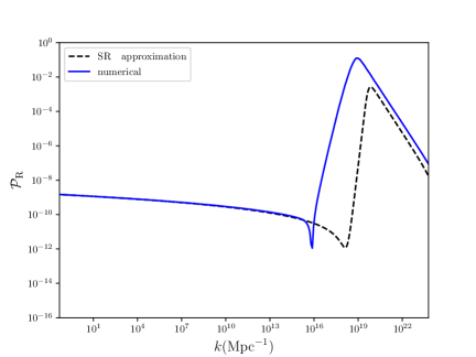
Figure 1: The curvature power spectrum $\mathcal{P}_{\mathcal{R}}(k)$ as a function of the wavenumber $k$, for $a=-1$, $b=22.35$, $c=0.065$, $\mu=2\times 10^{-5}$, $\lambda/\mu=0.3333449$ and $\phi_{0}=0.4295$ in Planck units. The black dashed curve represents the slow-roll (SR) approximation for $\mathcal{P}_{\mathcal{R}}(k)$, while the blue solid curve is the exact one after the numerical integration of the Mukhanov-Sasaki equation.

Primordial black hole formation – We will recap briefly now the fundamentals of PBH formation. PBHs form out of the collapse of local overdensity regions when the energy density contrast of the collapsing overdensity becomes greater than a critical threshold $\delta_{\mathrm{c}}$ Harada et al. (2013); Musco et al. (2021). At the end, working within the context of peak theory Bardeen et al. (1986) one can straightforwardly show that the PBH mass function, defined as the energy density contribution of PBHs per logarithmic mass $\beta(M)\equiv\frac{1}{\rho_{\mathrm{tot}}}\frac{\mathrm{d}\rho_{\mathrm{PBH}}}{\mathrm{d}\ln M}$, is given by Young et al. (2019)

$$\beta(M)=\int_{\nu_{\mathrm{c}}}^{\frac{4}{3\sigma}}\mathrm{d}\nu\frac{\mathcal{K}}{4\pi^{2}}\left(\nu\sigma-\frac{3}{8}\nu^{2}\sigma^{2}-\delta_{\mathrm{c}}\right)^{\gamma}\frac{\mu^{3}\nu^{3}}{\sigma^{3}}e^{-\nu^{2}/2},$$ (11)

with $\nu_{\mathrm{c}}=\delta_{\mathrm{c},l}/\sigma$ and $\delta_{\mathrm{c},l}=\frac{4}{3}\left(1-\mathchoice{{\hbox{$\displaystyle\sqrt{\frac{2-3\delta_{\mathrm{c}}}{2}\,}$}\lower 0.4pt\hbox{\vrule height=11.37221pt,depth=-9.09781pt}}}{{\hbox{$\textstyle\sqrt{\frac{2-3\delta_{\mathrm{c}}}{2}\,}$}\lower 0.4pt\hbox{\vrule height=7.97777pt,depth=-6.38225pt}}}{{\hbox{$\scriptstyle\sqrt{\frac{2-3\delta_{\mathrm{c}}}{2}\,}$}\lower 0.4pt\hbox{\vrule height=5.94443pt,depth=-4.75557pt}}}{{\hbox{$\scriptscriptstyle\sqrt{\frac{2-3\delta_{\mathrm{c}}}{2}\,}$}\lower 0.4pt\hbox{\vrule height=5.94443pt,depth=-4.75557pt}}}\right)$ being the linear PBH formation threshold. The parameters $\sigma^{2}$ and $\mu^{2}$ are the smoothed power spectrum and its first moment defined as

$$\sigma^{2} \equiv\frac{4(1+w)^{2}}{(5+3w)^{2}}\int_{0}^{\infty}\frac{\mathrm{d}k}{k}(kR)^{4}\tilde{W}^{2}(k,R)\mathcal{P}_{\mathcal{R}}(k),$$ (12)

$$\mu^{2} \equiv\frac{4(1+w)^{2}}{(5+3w)^{2}}\int_{0}^{\infty}\frac{\mathrm{d}k}{k}(kR)^{4}\tilde{W}^{2}(k,R)\mathcal{P}_{\mathcal{R}}(k)\left(\frac{k}{aH}\right)^{2},$$ (13)

with $w$ being the equation-of-state parameter of the dominant background component, and $\tilde{W}^{2}(k,R)$ the Fourier transform of the Gaussian window function $\tilde{W}(R,k)=e^{-k^{2}R^{2}/2}$ Young et al. (2014); Young (2019).

We should highlight here that in Eq. (11) we have accounted for the non-linear relation between the energy density contrast $\delta$ and the comoving curvature perturbation $\mathcal{R}$ giving rise to an inherent primordial non-Gaussianity of the $\delta$ field De Luca et al. (2019); Young et al. (2019), as well as for the fact that the PBH mass is given by the critical collapse scaling law $M_{\mathrm{PBH}}=M_{\mathrm{H}}\mathcal{K}(\delta-\delta_{\mathrm{c}})^{\gamma}$ Niemeyer and Jedamzik (1998); Musco et al. (2009), where $M_{\mathrm{H}}$ is the mass within the cosmological horizon at PBH formation time, and $\gamma$ is the critical exponent at the time of PBH formation (for PBH formation in the RD era $\gamma\simeq 0.36$). Regarding the parameter $\mathcal{K}$ we work with its representative value $\mathcal{K}\simeq 4$ Musco et al. (2009), while concerning the value of the PBH formation threshold $\delta_{\mathrm{c}}$, we accounted for its dependence on the shape of the collapsing curvature power spectrum. At the end, following the formalism developed in Musco et al. (2021) we found it equal to $\delta_{\mathrm{c}}\simeq 0.505$.

The primordial black hole gas – Working within Wess-Zumino type no-scale supergravity Ellis et al. (2013b), we obtain an enhanced curvature power spectrum which is broader compared to the Dirac-monochromatic case (see Fig. 1) but still sharp giving rise naturally to nearly monochromatic PBH mass distributions $\beta(M)$ [See the left panel of Fig. 2]. One then obtains in principle a “gas” of PBHs with different masses lying within the mass range $[10\mathrm{g},10^{9}\mathrm{g}]$, hence evaporating before BBN Kawasaki et al. (1999). Most of them however will have a common mass associated to the peak of the primordial curvature power spectrum. Due to the effect of Hawking radiation, each PBH will loose its mass with the dynamical evolution of the latter being given by $M(t)=M_{\mathrm{f}}\left\{1-\frac{t-t_{\mathrm{f}}}{\Delta t_{\mathrm{evap}}(M_{\mathrm{f}})}\right\}^{1/3}$ Hawking (1974), where $t_{\mathrm{f}}$ is the PBH formation time and $\Delta t_{\mathrm{evap}}$ is the black hole evaporation time scaling with the black hole mass as $\Delta t_{\mathrm{evap}}(M_{\mathrm{f}})=\frac{160}{\pi g_{\mathrm{*}}}\frac{M^{3}_{\mathrm{f}}}{M_{\scriptscriptstyle{\mathrm{Pl}}}^{4}}$, with $g_{\mathrm{*}}$ being the effective number of relativistic degrees of freedom.

If now $\bar{\beta}$ denotes the mass fraction without accounting for Hawking evaporation, one can recast $\Omega_{\mathrm{PBH}}(t)$ as

$$\Omega_{\mathrm{PBH}}(t)=\int_{M_{\mathrm{min}}}^{M_{\mathrm{max}}}\bar{\beta}\left(M,t\right)\left\{1-\frac{t-t_{\mathrm{ini}}}{\Delta t_{\mathrm{evap}}(M_{\mathrm{f}})}\right\}^{1/3}\mathrm{d}\ln M\,,$$ (14)

where $t_{\mathrm{ini}}$ denotes the initial time in our dynamical evolution, which is basically the formation time of the smallest PBH mass considered. Regarding now the lower mass bound $M_{\mathrm{min}}$, it will be given as the maximum between the minimum PBH mass at formation and the PBH mass evaporating at time $t$ defined as $M_{\mathrm{evap}}(t)\equiv\left(\frac{\pi g_{\mathrm{*}}M_{\scriptscriptstyle{\mathrm{Pl}}}^{4}\Delta t_{\mathrm{evap}}}{160}\right)^{1/3}$. One then obtains that $M_{\mathrm{min}}=\max[M_{\mathrm{f,min}},M_{\mathrm{evap}}(t)]$.

After integrating numerically Eq. (14) we obtain the PBH and the radiation background energy densities, which are depicted in the right panel of Fig. 2. As we observe, the PBH abundance increases with time due to the effect of cosmic expansion, since at early times when $\Omega_{\mathrm{PBH}}\ll 1$ and Hawking radiation is negligible, $\Omega_{\mathrm{PBH}}=\frac{\rho_{\mathrm{PBH}}}{\rho_{\mathrm{tot}}}\propto a^{-3}/a^{-4}\propto a$, dominating in this way for a transient period the Universe’s energy budget. Then, at some point Hawking evaporation becomes the driving force in the dynamics of $\Omega_{\mathrm{PBH}}$ and the PBH abundance starts to decrease. Here, it is important to stress that, as one may notice from the right panel of Fig. 2, the transition from the eMD era driven by PBHs to the late RD (lRD) era lasts only one e-fold, hence one can treat the transition as instantaneous. This is related to the fact that the PBH mass function at formation can be treated as monochromatic. From the left panel of Fig. 2 one can clearly see that the PBH mass function at formation $\beta(M)$ decays $11$ orders of magnitude in less than two decades in $M$.

We should mention at this point that the initial reheating temperature is determined by the energy scale at the end of inflation considering instantaneous reheating, i.e. $\rho_{\mathrm{inf}}=g_{*}\frac{\pi^{2}}{30}T^{4}_{\mathrm{reh}}$, where $g_{*}$ is the effective number of relativistic degrees of freedom. For our inflationary setup, we find after solving numerically the Klein-Gordon equation, that inflation ends when $\rho^{1/4}_{\mathrm{tot}}=\rho_{\mathrm{inf}}=10^{15}\mathrm{GeV}$. In contrast, the second reheating happens when PBHs evaporate, just before BBN, at around $1\mathrm{MeV}$.

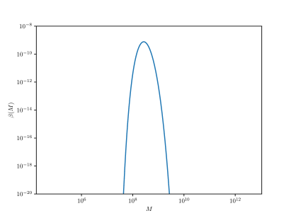
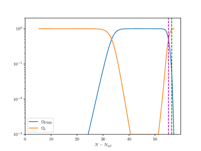
Figure 2: Left Panel: The PBH mass function at formation Eq. (11). Right Panel: The dynamical evolution of the background PBH and radiation energy densities as a function of the e-folds passed from the end of inflation. The magenta vertical dashed line denotes the time of the onset of the radiation-dominated era, namely when $\Omega_{\mathrm{r}}=0.5$, whereas the green dashed vertical line stands for the time when $\Omega_{\mathrm{r}}=0.95$, namely when we are fully back to the radiation-dominated Universe. For both panels, we used $a=-1$, $b=22.35$, $c=0.065$, $\mu=2\times 10^{-5}$, $\lambda/\mu=0.3333449$ and $\phi_{0}=0.4295$ in Planck units.

Scalar induced gravitational waves – Let us now derive the gravitational waves induced due to second order gravitational interactions by first order curvature perturbations Matarrese et al. (1993, 1994, 1998); Mollerach et al. (2004) [See Domènech (2021) for a review]. Working in the Newtonian gauge  the perturbed metric is written as $\mathrm{d}s^{2}=a^{2}(\eta)\left\{-(1+2\Phi)\mathrm{d}\eta^{2}+\left[(1-2\Phi)\delta_{ij}+\frac{h_{ij}}{2}\right]\mathrm{d}x^{i}\mathrm{d}x^{j}\right\}$, where $\Phi$ is the first order Bardeen gravitational potential and $h_{ij}$ stands for the second order tensor perturbation. Then, by performing a Fourier transform of the tensor perturbation, the equation of motion for $h_{\boldsymbol{k}}$ will be written as

$$h_{\boldsymbol{k}}^{s,\prime\prime}+2\mathcal{H}h_{\boldsymbol{k}}^{s,\prime}+k^{2}h^{s}_{\boldsymbol{k}}=4S^{s}_{\boldsymbol{k}},$$ (15)

where $s=(+),(\times)$, $\mathcal{H}$ is the conformal Hubble parameter and while the polarization tensors $e^{s}_{ij}(k)$ are the standard ones Espinosa et al. (2018) and the source function $S^{s}_{\boldsymbol{k}}$ is given by 

$$\!\!\!\!\!\!\!\!\!\!\!\!\!\!S^{s}_{\boldsymbol{k}}=\int\frac{\mathrm{d}^{3}{\boldsymbol{q}}}{(2\pi)^{3/2}}e^{s}_{ij}({\boldsymbol{k}})q_{i}q_{j}\Big{[}2\Phi_{\boldsymbol{q}}\Phi_{\boldsymbol{k-q}}$$

$$\!\!\!\!\!\!\!\!+\frac{4}{3(1\!+\!w_{\mathrm{tot}})}(\mathcal{H}^{-1}\Phi_{\boldsymbol{q}}^{\prime}+\Phi_{\boldsymbol{q}})(\mathcal{H}^{-1}\Phi_{\boldsymbol{k-q}}^{\prime}+\Phi_{\boldsymbol{k-q}})\Big{]}.$$ (16)

After a long but straightforward calculation, one obtains a tensor power spectrum $\mathcal{P}_{h}(\eta,k)$ reading as Ananda et al. (2007); Baumann et al. (2007); Kohri and Terada (2018); Espinosa et al. (2018)

$$\!\!\!\!\!\!\!\!\!\mathcal{P}^{(s)}_{h}(\eta,k)=4\int_{0}^{\infty}\mathrm{d}v\int_{|1-v|}^{1+v}\mathrm{d}u\!\left[\frac{4v^{2}-(1\!+\!v^{2}\!-\!u^{2})^{2}}{4uv}\right]^{2}$$

$$\ \ \ \ \ \ \ \ \ \ \ \ \ \ \ \ \ \ \ \ \ \ \ \ \ \ \cdot I^{2}(u,v,x)\mathcal{P}_{\Phi}(kv)\mathcal{P}_{\Phi}(ku)\,,$$ (17)

where the two auxiliary variables $u$ and $v$ are defined as $u\equiv|{\boldsymbol{k}}-{\boldsymbol{q}}|/k$ and $v\equiv q/k$, and the kernel function $I(u,v,x)$ is a complicated function containing information for the transition between the eMD era driven by PBHs and the lRD era Kohri and Terada (2018); Inomata et al. (2019a, b, 2020); Papanikolaou (2022). Hence, we can recast the GW spectral abundance defined as the GW energy density per logarithmic comoving scale as Maggiore (2000); Kohri and Terada (2018)

$$\Omega_{\mathrm{GW}}(\eta,k)\equiv\frac{1}{\bar{\rho}_{\mathrm{tot}}}\frac{\mathrm{d}\rho_{\mathrm{GW}}(\eta,k)}{\mathrm{d}\ln k}=\frac{1}{24}\left(\frac{k}{\mathcal{H}(\eta)}\right)^{2}\overline{\mathcal{P}^{(s)}_{h}(\eta,k)}.$$ (18)

Finally, considering that the radiation energy density reads as $\rho_{r}=\frac{\pi^{2}}{30}g_{*\mathrm{\rho}}T_{\mathrm{r}}^{4}$ and that the temperature of the primordial plasma $T_{\mathrm{r}}$ scales as $T_{\mathrm{r}}\propto g^{-1/3}_{*\mathrm{S}}a^{-1}$, one finds that the GW spectral abundance at our present epoch reads as

$$\Omega_{\mathrm{GW}}(\eta_{0},k)=\Omega^{(0)}_{r}\frac{g_{*\mathrm{\rho},\mathrm{*}}}{g_{*\mathrm{\rho},0}}\left(\frac{g_{*\mathrm{S},\mathrm{0}}}{g_{*\mathrm{S},\mathrm{*}}}\right)^{4/3}\Omega_{\mathrm{GW}}(\eta_{\mathrm{*}},k),$$ (19)

where $g_{*\mathrm{\rho}}$ and $g_{*\mathrm{S}}$ denote the energy and entropy relativistic degrees of freedom. Note that the reference conformal time $\eta_{\mathrm{*}}$ in the case of an instantaneous transition from the eMD to the lRD era should be of $\mathcal{O}(1)\eta_{r}$ Inomata et al. (2019a, 2020). In the case of gradual transition, $\eta_{\mathrm{*}}\sim(1-4)\eta_{\mathrm{r}}$ in order for $\Phi$ to have sufficiently decayed and the tensor modes to be considered as freely propagating GWs Inomata et al. (2019b); Papanikolaou (2022).

The relevant gravitational-wave sources – We can now concentrate on the different sources of GWs considered within this work. In particular, for a sharply peaked primordial curvature power spectrum like ours, GWs are sourced through two different mechanisms Bhaumik et al. (2022, 2023a): Firstly, by the primordial inflationary curvature perturbations during the early RD (eRD) era, and later by early isocurvature PBH Poisson fluctuations during the eMD and the lRD eras. Given now the suddenness of the transition from the eMD to the lRD era, the induced GWs are resonantly amplified due to the large amplitude of the oscillations of the curvature perturbations after the sudden transition Inomata et al. (2019a, 2020); Domènech et al. (2021a).

To be more explicit, the first GW production mechanism gives rise to two GW peaks Bhaumik et al. (2023b). The first peak is related to GWs induced by the enhanced primordial curvature power spectrum around the PBH scale, namely around $k=10^{19}\mathrm{Mpc}^{-1}$, which is associated to PBH formation. In order to extract this GW spectrum, one needs to use the kernel function $I(u,v,x)$ during an eRD era Kohri and Terada (2018) when the PBHs form and evolve the GW spectral abundance through the subsequent eMD era driven by PBHs, during which the GW spectrum is diluted as $\Omega_{\mathrm{GW}}\propto\rho_{\mathrm{GW}}/\rho_{\mathrm{PBH}}\propto a^{-4}/a^{-3}\propto 1/a$. At the end, one obtains that the induced GW due to PBH formation can be recast as

$$\Omega^{\mathrm{form}}_{\mathrm{GW}}(\eta_{0},k)=\frac{a_{\mathrm{d}}}{a_{\mathrm{evap}}}c_{g}\Omega^{(0)}_{\mathrm{r}}\Omega_{\mathrm{GW}}(\eta_{\mathrm{f}},k),$$ (20)

where $\eta_{\mathrm{f}}$ is the conformal PBH formation time, $c_{g}=\frac{g_{*\mathrm{\rho},\mathrm{*}}}{g_{*\mathrm{\rho},0}}\left(\frac{g_{*\mathrm{S},\mathrm{0}}}{g_{*\mathrm{S},\mathrm{*}}}\right)^{4/3}\sim 0.4$ and $a_{\mathrm{d}}$ and $a_{\mathrm{evap}}$ are respectively the scale factors at the onset of eMD era when PBHs dominate and the lRD era when PBHs evaporate. $\Omega_{\mathrm{GW}}(\eta_{\mathrm{f}},k)$ is derived from Eq. (18) at PBH formation time. One may naively expect from Eq. (17) and Eq. (18) that for sharply peaked primordial curvature power spectra as in our case: $\Omega_{\mathrm{GW}}\propto\mathcal{P}^{2}_{\Phi}\propto\mathcal{P}^{2}_{\mathcal{R}}$, since $\mathcal{R}=2\Phi/3$ in superhorizon scales Wands et al. (2000). At the end, for our fiducial choice of the inflationary parameters involved, the GW signal associated to PBH formation peaks at the $\mathrm{kHz}$ frequency range [See the yellow solid curve in Fig. 4].

Regarding now the second peak at $\mathrm{nHz}$, it is related to the resonant amplification of the curvature perturbation on scales entering the cosmological horizon during the eMD. In particular, the source of the enhancement leading to the $\mathrm{nHz}$ peak is the sudden transition from the eMD era to the lRD era. Specifically, during the transition the time derivative of the Bardeen potential goes very quickly from $\Phi^{\prime}=0$ (since in a MD era $\Phi=\mathrm{constant}$ ) to $\Phi^{\prime}\neq 0$ in the late RD era [See Inomata et al. (2019a); Domènech (2021) for more details.]. This entails a resonantly enhanced production of GWs sourced mainly by the $\mathcal{H}^{-2}\Phi^{\prime 2}$ term in Eq. (16).

Furthermore, since the sub-horizon energy density perturbations during a MD era scale linearly with the scale factor, i.e. $\delta\propto a$, one should ensure working within the perturbative regime. For this reason, we set a non-linear scale $k_{\mathrm{NL}}$ by requiring that $\delta_{\mathrm{k_{\mathrm{NL}}}}(\eta_{\mathrm{r}})=1$. In particular, following the analysis of Assadullahi and Wands (2009); Inomata et al. (2020), one can show that the non-linear cut-off scale  at which $\delta_{k_{\mathrm{NL}}}(\eta_{r})=1$ can be recast as

$$k_{\mathrm{NL}}\simeq\mathchoice{{\hbox{$\displaystyle\sqrt{\frac{5}{2}\,}$}\lower 0.4pt\hbox{\vrule height=9.66666pt,depth=-7.73337pt}}}{{\hbox{$\textstyle\sqrt{\frac{5}{2}\,}$}\lower 0.4pt\hbox{\vrule height=6.76666pt,depth=-5.41336pt}}}{{\hbox{$\scriptstyle\sqrt{\frac{5}{2}\,}$}\lower 0.4pt\hbox{\vrule height=4.83331pt,depth=-3.86667pt}}}{{\hbox{$\scriptscriptstyle\sqrt{\frac{5}{2}\,}$}\lower 0.4pt\hbox{\vrule height=4.83331pt,depth=-3.86667pt}}}\mathcal{P}^{-1/4}_{\mathcal{R}}(k_{\mathrm{NL}})\mathcal{H}(\eta_{r}).$$ (21)

Since within no-scale Supergravity we predict a Starobinsky-like inflationary setup with $n_{\mathrm{s}}=0.965$, we can assume as a first approximation a scale-invariant curvature power spectrum of amplitude $2.1\times 10^{-9}$ as imposed by Planck Aghanim et al. (2020), giving rise to $k_{\mathrm{NL}}\simeq 470/\eta_{\mathrm{r}}\simeq 235k_{\mathrm{r}}$ Inomata et al. (2019a),where $k_{\mathrm{r}}$ is the comoving scale crossing the cosmological horizon at the onset of the lRD era. Ultimately, the peak frequency of this $\mathrm{nHz}$ signal is associated with the non-linear comoving cut-off scale, $k_{\mathrm{NL}}=235k_{r}$, which depends on the PBH mass $M$ as Bhaumik et al. (2023b) $k_{\mathrm{r}}=2.1\times 10^{11}\left(\frac{M}{10^{4}\mathrm{g}}\right)^{-3/2}\mathrm{Mpc}^{-1}$ Bhaumik et al. (2023b). The peak frequency of this signal can now be calculated from the formula $f_{\mathrm{GW}}=\frac{ck_{\mathrm{NL}}}{2\pi a_{0}}$, with $c$ the speed of light and $a_{0}=1$. The end result is a $f$ peaking at $\mathrm{nHz}$.

Remarkably, this second peak that corresponds to scales much larger than the PBH scale peaks at the $\mathrm{nHz}$ frequency range and is in strong agreement with the NANOGrav/PTA data - See the blue solid curve in Fig. 4 as well as Fig. 3 where we have zoomed in the NANOGrav frequency range. This second resonant peak is derived by

$$\Omega^{\mathrm{res}}_{\mathrm{GW}}(\eta_{0},k)=c_{g}\Omega^{(0)}_{\mathrm{r}}\Omega_{\mathrm{GW}}(\eta_{\mathrm{lRD}},k),$$ (22)

where $\eta_{\mathrm{lRD}}$ stands for a time during lRD by which the curvature perturbations decouple from the tensor perturbations and one is met with freely propagating GWs. $\Omega_{\mathrm{GW}}(\eta_{\mathrm{lRD}},k)$ is derived from Eq. (18) where $I(u,v,x)=I_{\mathrm{lRD}}(u,v,x)$ Inomata et al. (2019a).

It is important to highlight here the possibility of later PBH formation due to the linear growth of the matter energy density perturbations during the PBH-driven eMD era. Interestingly enough, one expects a further PBH production similarly to PBH production from preheating Martin et al. (2020) as well as early inflaton structure formation Jedamzik et al. (2010); Hidalgo et al. (2023). The study of this interesting phenomenology is beyond the scope of this work and will be studied elsewhere.

Finally, we consider the GW spectrum induced by the gravitational potential of our PBH population itself. To elaborate, assuming that PBHs are randomly distributed at formation time (i.e. they have Poisson statistics) Desjacques and Riotto (2018); Moradinezhad Dizgah et al. (2019), their energy density is inhomogeneous while the total background radiation energy density is homogeneous. Therefore, the PBH energy density perturbation can be described by an isocurvature Poisson fluctuation Papanikolaou et al. (2021) which in the subsequent PBH domination era will be converted into an adiabatic curvature perturbation associated to a PBH gravitational potential $\Phi_{\mathrm{PBH}}$. This gravitational potential $\Phi_{\mathrm{PBH}}$ will be another source of induced GWs.  The power spectrum of $\Phi_{\mathrm{PBH}}$ can be recast as Papanikolaou et al. (2021):

$$\mathcal{P}_{\Phi_{\mathrm{PBH}}}(k)=\frac{2}{3\pi}\left(\frac{k}{k_{\rm{UV}}}\right)^{3}\left(5+\frac{4}{9}\frac{k^{2}}{k_{\rm{d}}^{2}}\right)^{-2},$$ (23)

where $k_{\mathrm{d}}$ stands for the comoving scale re-entering the cosmological horizon at PBH domination time and $k_{\mathrm{UV}}$ is a UV cutoff scale defined as $k_{\mathrm{UV}}\equiv a/\bar{r}$, where $\bar{r}$ corresponds to the mean PBH separation distance. One then can compute the relevant tensor power spectrum through Eq. (17) where now $\mathcal{P}_{\Phi}(k)$ should be replaced with $\mathcal{P}_{\Phi_{\mathrm{PBH}}}(k)$. One would expect that this GW signal will peak at $k_{\mathrm{d}}$, namely the scale crossing the cosmological horizon at the onset of the PBH domination era, since as one may see from Eq. (23), $\mathcal{P}_{\Phi_{\mathrm{PBH}}}(k)$ peaks at $k_{\mathrm{d}}$. However, due to a $k^{8}$ dependence of the kernel $I^{2}_{\mathrm{lRD,res}}(u,v,x_{\mathrm{evap}})$, the peak of the GW signal induced by PBH Poisson fluctuations is shifted from $k_{\mathrm{d}}$ to $k_{\mathrm{UV}}$. As one can see from the green solid line of Fig. 4, for our fiducial choice for the inflationary parameters at hand, this GW signal lies within the $\mathrm{Hz}$ frequency range with an amplitude of the order of $10^{-14}$, being close to sensitivity bands of the Einstein Telescope (ET) Maggiore et al. (2020) and Big Bang Observer (BBO) Harry et al. (2006).

It is noteworthy that since GWs generated before BBN can act as an extra relativistic component, they will contribute to the effective number of extra neutrino species $\Delta N_{\mathrm{eff}}$, which is severely constrained by BBN and CMB observations as $\Delta N_{\mathrm{eff}}<0.3$ Aghanim et al. (2020). This upper bound constraint on $\Delta N_{\mathrm{eff}}$ is translated to an upper bound on the GW amplitude which reads as Smith et al. (2006); Caprini and Figueroa (2018) as $\Omega_{\mathrm{GW,0}}h^{2}\leq 6.9\times 10^{-6}$ . This upper bound on $\Omega_{\mathrm{GW}}$ is shown with the horizontal black dashed line in Fig. 4.

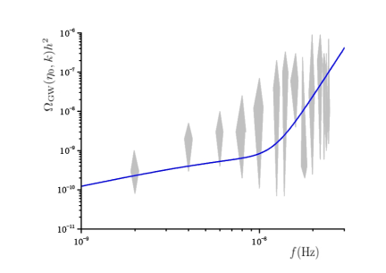
Figure 3: The stochastic GW background (GW density parameter as a function of the frequency) induced by resonantly amplified inflationary perturbations and arising from Wess-Zumino no-scale Supergravity with the extended Kähler potential (4) for $a=-1$, $b=22.35$, $c=0.065$, $\mu=2\times 10^{-5}$, $\lambda/\mu=0.3333449$ and $\phi_{0}=0.4295$ in Planck units - corresponding to $M_{\mathrm{PBH}}=7\times 10^{8}\mathrm{g}$ and $\Omega_{\mathrm{PBH,f}}=10^{-9}$ - on top of the 15-year NANOGrav data.

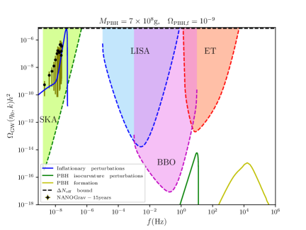
Figure 4: The stochastic three-peaked GW background induced by inflationary adiabatic (solid blue and yellow curves) and PBH isocurvature perturbations (solid green curve) arising from Wess-Zumino no-scale Supergravity with the extended Kähler potential (4) for $a=-1$, $b=22.35$, $c=0.065$, $\mu=2\times 10^{-5}$, $\lambda/\mu=0.3333449$ and $\phi_{0}=0.4295$ in Planck units and corresponding to $M_{\mathrm{PBH}}=7\times 10^{8}\mathrm{g}$ and $\Omega_{\mathrm{PBH,f}}=10^{-9}$. On the top of our theoretical prediction for the induced stochastic GW background we show the 15-year NANOGrav GW data, as well as the sensitivities of SKA Janssen et al. (2015), LISA Auclair et al. (2022), BBO Harry et al. (2006) and ET Maggiore et al. (2020) GW experiments. In the horizontal black dashed line, we show also the upper bound on $\Omega_{\mathrm{GW,0}}h^{2}\leq 6.9\times 10^{-6}$ coming from the upper bound constraint on $\Delta N_{\mathrm{eff}}$ from CMB and BBN observations Smith et al. (2006).

Conclusions – In this Letter, we showed that no-scale Supergravity, being the low-energy limit of Superstring theory, seems to accomplish three main achievements. Firstly, it provides a successful Starobinsky-like inflation realization with all the desired observational predictions regarding $n_{\mathrm{s}}$ and $r$ Antoniadis et al. (2021); Ellis et al. (2013b). Secondly, it can naturally lead to inflection-point inflationary potentials giving rise to sharp mass distributions of microscopic PBHs triggering an eMD era before BBN, and thirdly it can induce through second order gravitational interactions a distinctive three-peaked GW signal.

In particular, working within the context of Wess-Zumino no-scale Supergravity we found i) a $\mathrm{nHz}$ GW signal induced by enhanced inflationary adiabatic perturbations and resonantly amplified due to the sudden transition from a eMD era driven by “no-scale" microscopic PBHs to the standard RD era, being as well within the error-bars of the recently PTA GW data, ii) a $\mathrm{Hz}$ GW signal induced by the PBH isocurvature energy density perturbations and close to the GW sensitivity bands of ET and BBO GW experiments and iii) a $\mathrm{kHz}$ GW signal associated to the PBH formation. Remarkably, a simultaneous detection of all three $\mathrm{nHz}$, $\mathrm{Hz}$ and $\mathrm{kHz}$ GW peaks can constitute a potential observational signature for no-scale Supergravity.

It is important to highlight here that we extracted the aforementioned three-peaked induced GW signal within the context of Wess-Zumino no-scale Supergravity. However, due to the unified treatment of Starobinsky-like inflationary avatars of $SU(2,1)/SU(2)\times U(1)$ no-scale supergravity models Ellis et al. (2013a) which exhibit $6$ specific equivalence classes Ellis et al. (2019), one expects that the three-peaked GW signal induced by inflationary adiabatic and PBH isocurvture perturbations will be a generic feature of any $SU(2,1)/SU(2)\times U(1)$ no-scale Supergravity theory with an appropriately deformed Kähler potential, e.g. of the form Eq. (4), leading to inflection-point inflationary potentials.

One should mention as well that in principle a three-peaked GW signal is a generic feature of any model predicting formation of ultra-light PBHs dominating the early Universe. However, the particular three-peaked GW signal found here, at $\mathrm{nHz}$, $\mathrm{Hz}$ and $\mathrm{kHz}$, is a a pure byproduct of the no-scale Wess-Zumino inflection-point inflationary potential and consistent with the recently released PTA GW data. Thus, its detection will constitute a potential observational signature of no-scale Supergravity.

Finally, we need to note that in the case of broader PBH mass functions produced within no-scale Supergravity, one expects an oscillatory GW signal due to the gradualness of the transition from the eMD to the lRD era Inomata et al. (2019b); Papanikolaou (2022). Such oscillatory GW signals have been proposed as well in other theoretical constructions [See Braglia et al. (2021); Fumagalli et al. (2021a, b, 2022); Mavromatos et al. (2022)] and it will be quite tentative to distinguish between them experimentally. Finally, we should mention that a proper statistical comparison between no-scale Supergravity models and GW data will place strong constraints on the relevant parameter space involved. Such an analysis is in progress and will be published elsewhere.

Acknowledgements – The authors thank Ioanna Stamou, Valerie Domcke, Ninlanjandev Bhaumik, Rajeev Kumar Jain and Marek Lewicki for useful and stimulating discussions. The work of DVN was supported in part by the DOE grant DE-FG02-13ER42020 at Texas A&M University and in part by the Alexander S. Onassis Public Benefit Foundation. SB, ENS, TP and CT acknowledge the contribution of the LISA CosWG and the COST Actions CA18108 “Quantum Gravity Phenomenology in the multi-messenger approach” and CA21136 “Addressing observational tensions in cosmology with systematics and fundamental physics (CosmoVerse)”. TP and CT acknowledge as well financial support from the Foundation for Education and European Culture in Greece and A.G. Leventis Foundation respectively.

References

- Afzal et al. (2023) A. Afzal et al. (NANOGrav), Astrophys. J. Lett. 951, L11 (2023), arXiv:2306.16219 [astro-ph.HE] .
- Agazie et al. (2023) G. Agazie et al. (NANOGrav), Astrophys. J. Lett. 952, L37 (2023), arXiv:2306.16220 [astro-ph.HE] .
- Ellis et al. (2023) J. Ellis, M. Fairbairn, G. Franciolini, G. Hütsi, A. Iovino, M. Lewicki, M. Raidal, J. Urrutia, V. Vaskonen, and H. Veermäe, (2023), arXiv:2308.08546 [astro-ph.CO] .
- Cremmer et al. (1983) E. Cremmer, S. Ferrara, C. Kounnas, and D. V. Nanopoulos, Phys. Lett. B 133, 61 (1983).
- Ellis et al. (1984a) J. R. Ellis, A. B. Lahanas, D. V. Nanopoulos, and K. Tamvakis, Phys. Lett. B 134, 429 (1984a).
- Ellis et al. (1984b) J. R. Ellis, C. Kounnas, and D. V. Nanopoulos, Nucl. Phys. B 247, 373 (1984b).
- Lahanas and Nanopoulos (1987) A. B. Lahanas and D. V. Nanopoulos, Phys. Rept. 145, 1 (1987).
- Freedman and Van Proeyen (2012) D. Z. Freedman and A. Van Proeyen, Supergravity (Cambridge Univ. Press, Cambridge, UK, 2012).
- Witten (1985) E. Witten, Phys. Lett. B 155, 151 (1985).
- Dine et al. (1985) M. Dine, R. Rohm, N. Seiberg, and E. Witten, Phys. Lett. B 156, 55 (1985).
- Antoniadis et al. (1987) I. Antoniadis, J. R. Ellis, E. Floratos, D. V. Nanopoulos, and T. Tomaras, Phys. Lett. B 191, 96 (1987).
- Ellis et al. (2013a) J. Ellis, D. V. Nanopoulos, and K. A. Olive, JCAP 10, 009 (2013a), arXiv:1307.3537 [hep-th] .
- Kounnas et al. (2015) C. Kounnas, D. Lüst, and N. Toumbas, Fortsch. Phys. 63, 12 (2015), arXiv:1409.7076 [hep-th] .
- Antoniadis et al. (2021) I. Antoniadis, D. V. Nanopoulos, and J. Rizos, JCAP 03, 017 (2021), arXiv:2011.09396 [hep-th] .
- Antoniadis et al. (2022) I. Antoniadis, D. V. Nanopoulos, and J. Rizos, Eur. Phys. J. C 82, 377 (2022), arXiv:2112.01211 [hep-th] .
- Ellis et al. (2013b) J. Ellis, D. V. Nanopoulos, and K. A. Olive, Phys. Rev. Lett. 111, 111301 (2013b), [Erratum: Phys.Rev.Lett. 111, 129902 (2013)], arXiv:1305.1247 [hep-th] .
- Inomata et al. (2023) K. Inomata, M. Braglia, X. Chen, and S. Renaux-Petel, JCAP 04, 011 (2023), arXiv:2211.02586 [astro-ph.CO] .
- Kristiano and Yokoyama (2022) J. Kristiano and J. Yokoyama, (2022), arXiv:2211.03395 [hep-th] .
- Choudhury et al. (2023a) S. Choudhury, S. Panda, and M. Sami, Phys. Lett. B 845, 138123 (2023a), arXiv:2302.05655 [astro-ph.CO] .
- Choudhury et al. (2023b) S. Choudhury, S. Panda, and M. Sami, (2023b), arXiv:2303.06066 [astro-ph.CO] .
- Choudhury et al. (2023c) S. Choudhury, M. R. Gangopadhyay, and M. Sami, (2023c), arXiv:2301.10000 [astro-ph.CO] .
- Franciolini et al. (2023) G. Franciolini, A. Iovino, Junior., M. Taoso, and A. Urbano, (2023), arXiv:2305.03491 [astro-ph.CO] .
- Firouzjahi and Riotto (2023) H. Firouzjahi and A. Riotto, (2023), arXiv:2304.07801 [astro-ph.CO] .
- Hooper et al. (2019) D. Hooper, G. Krnjaic, and S. D. McDermott, JHEP 08, 001 (2019), arXiv:1905.01301 [hep-ph] .
- Papanikolaou (2023) T. Papanikolaou, in CORFU2022 (2023) arXiv:2303.00600 [astro-ph.CO] .
- Nanopoulos et al. (2020) D. V. Nanopoulos, V. C. Spanos, and I. D. Stamou, Phys. Rev. D 102, 083536 (2020), arXiv:2008.01457 [astro-ph.CO] .
- (27) J. R. Ellis, C. Kounnas, and D. V. Nanopoulos, Phys. Lett. B 143, 410.
- Aghanim et al. (2020) N. Aghanim et al. (Planck), Astron. Astrophys. 641, A6 (2020), [Erratum: Astron.Astrophys. 652, C4 (2021)], arXiv:1807.06209 [astro-ph.CO] .
- Mukhanov et al. (1992) V. F. Mukhanov, H. A. Feldman, and R. H. Brandenberger, Phys. Rept. 215, 203 (1992).
- Carr et al. (2020) B. Carr, K. Kohri, Y. Sendouda, and J. Yokoyama, (2020), arXiv:2002.12778 [astro-ph.CO] .
- Ellis et al. (2019) J. Ellis, D. V. Nanopoulos, K. A. Olive, and S. Verner, JHEP 03, 099 (2019), arXiv:1812.02192 [hep-th] .
- Cole et al. (2023) P. S. Cole, A. D. Gow, C. T. Byrnes, and S. P. Patil, JCAP 08, 031 (2023), arXiv:2304.01997 [astro-ph.CO] .
- Harada et al. (2013) T. Harada, C.-M. Yoo, and K. Kohri, Phys. Rev. D88, 084051 (2013), [Erratum: Phys. Rev.D89,no.2,029903(2014)], arXiv:1309.4201 [astro-ph.CO] .
- Musco et al. (2021) I. Musco, V. De Luca, G. Franciolini, and A. Riotto, Phys. Rev. D 103, 063538 (2021), arXiv:2011.03014 [astro-ph.CO] .
- Bardeen et al. (1986) J. M. Bardeen, J. R. Bond, N. Kaiser, and A. S. Szalay, Astrophys. J. 304, 15 (1986).
- Young et al. (2019) S. Young, I. Musco, and C. T. Byrnes, JCAP 11, 012 (2019), arXiv:1904.00984 [astro-ph.CO] .
- Young et al. (2014) S. Young, C. T. Byrnes, and M. Sasaki, JCAP 1407, 045 (2014), arXiv:1405.7023 [gr-qc] .
- Young (2019) S. Young, Int. J. Mod. Phys. D 29, 2030002 (2019), arXiv:1905.01230 [astro-ph.CO] .
- De Luca et al. (2019) V. De Luca, G. Franciolini, A. Kehagias, M. Peloso, A. Riotto, and C. Ünal, JCAP 07, 048 (2019), arXiv:1904.00970 [astro-ph.CO] .
- Niemeyer and Jedamzik (1998) J. C. Niemeyer and K. Jedamzik, Phys. Rev. Lett. 80, 5481 (1998), arXiv:astro-ph/9709072 [astro-ph] .
- Musco et al. (2009) I. Musco, J. C. Miller, and A. G. Polnarev, Class. Quant. Grav. 26, 235001 (2009), arXiv:0811.1452 [gr-qc] .
- Kawasaki et al. (1999) M. Kawasaki, K. Kohri, and N. Sugiyama, Phys. Rev. Lett. 82, 4168 (1999), arXiv:astro-ph/9811437 .
- Hawking (1974) S. W. Hawking, Nature 248, 30 (1974).
- Matarrese et al. (1993) S. Matarrese, O. Pantano, and D. Saez, Phys. Rev. D 47, 1311 (1993).
- Matarrese et al. (1994) S. Matarrese, O. Pantano, and D. Saez, Phys. Rev. Lett. 72, 320 (1994), arXiv:astro-ph/9310036 .
- Matarrese et al. (1998) S. Matarrese, S. Mollerach, and M. Bruni, Phys. Rev. D 58, 043504 (1998), arXiv:astro-ph/9707278 .
- Mollerach et al. (2004) S. Mollerach, D. Harari, and S. Matarrese, Phys. Rev. D 69, 063002 (2004), arXiv:astro-ph/0310711 .
- Domènech (2021) G. Domènech, Universe 7, 398 (2021), arXiv:2109.01398 [gr-qc] .
- Hwang et al. (2017) J.-C. Hwang, D. Jeong, and H. Noh, Astrophys. J. 842, 46 (2017), arXiv:1704.03500 [astro-ph.CO] .
- Tomikawa and Kobayashi (2020) K. Tomikawa and T. Kobayashi, Phys. Rev. D 101, 083529 (2020), arXiv:1910.01880 [gr-qc] .
- De Luca et al. (2020) V. De Luca, G. Franciolini, A. Kehagias, and A. Riotto, JCAP 03, 014 (2020), arXiv:1911.09689 [gr-qc] .
- Inomata and Terada (2020) K. Inomata and T. Terada, Phys. Rev. D 101, 023523 (2020), arXiv:1912.00785 [gr-qc] .
- Espinosa et al. (2018) J. R. Espinosa, D. Racco, and A. Riotto, JCAP 1809, 012 (2018), arXiv:1804.07732 [hep-ph] .
- Cai et al. (2019) R.-g. Cai, S. Pi, and M. Sasaki, Phys. Rev. Lett. 122, 201101 (2019), arXiv:1810.11000 [astro-ph.CO] .
- Chen et al. (2023) C. Chen, A. Ota, H.-Y. Zhu, and Y. Zhu, Phys. Rev. D 107, 083518 (2023), arXiv:2210.17176 [astro-ph.CO] .
- Ananda et al. (2007) K. N. Ananda, C. Clarkson, and D. Wands, Phys. Rev. D75, 123518 (2007), arXiv:gr-qc/0612013 [gr-qc] .
- Baumann et al. (2007) D. Baumann, P. J. Steinhardt, K. Takahashi, and K. Ichiki, Phys. Rev. D76, 084019 (2007), arXiv:hep-th/0703290 [hep-th] .
- Kohri and Terada (2018) K. Kohri and T. Terada, Phys. Rev. D97, 123532 (2018), arXiv:1804.08577 [gr-qc] .
- Inomata et al. (2019a) K. Inomata, K. Kohri, T. Nakama, and T. Terada, Phys. Rev. D 100, 043532 (2019a), arXiv:1904.12879 [astro-ph.CO] .
- Inomata et al. (2019b) K. Inomata, K. Kohri, T. Nakama, and T. Terada, JCAP 10, 071 (2019b), arXiv:1904.12878 [astro-ph.CO] .
- Inomata et al. (2020) K. Inomata, M. Kawasaki, K. Mukaida, T. Terada, and T. T. Yanagida, Phys. Rev. D 101, 123533 (2020), arXiv:2003.10455 [astro-ph.CO] .
- Papanikolaou (2022) T. Papanikolaou, JCAP 10, 089 (2022), arXiv:2207.11041 [astro-ph.CO] .
- Maggiore (2000) M. Maggiore, Phys. Rept. 331, 283 (2000), arXiv:gr-qc/9909001 [gr-qc] .
- Bhaumik et al. (2022) N. Bhaumik, A. Ghoshal, and M. Lewicki, JHEP 07, 130 (2022), arXiv:2205.06260 [astro-ph.CO] .
- Bhaumik et al. (2023a) N. Bhaumik, A. Ghoshal, R. K. Jain, and M. Lewicki, JHEP 05, 169 (2023a), arXiv:2212.00775 [astro-ph.CO] .
- Domènech et al. (2021a) G. Domènech, C. Lin, and M. Sasaki, JCAP 04, 062 (2021a), arXiv:2012.08151 [gr-qc] .
- Bhaumik et al. (2023b) N. Bhaumik, R. K. Jain, and M. Lewicki, (2023b), arXiv:2308.07912 [astro-ph.CO] .
- Wands et al. (2000) D. Wands, K. A. Malik, D. H. Lyth, and A. R. Liddle, Phys.Rev. D62, 043527 (2000), arXiv:astro-ph/0003278 [astro-ph] .
- Assadullahi and Wands (2009) H. Assadullahi and D. Wands, Phys. Rev. D 79, 083511 (2009), arXiv:0901.0989 [astro-ph.CO] .
- Martin et al. (2020) J. Martin, T. Papanikolaou, L. Pinol, and V. Vennin, JCAP 05, 003 (2020), arXiv:2002.01820 [astro-ph.CO] .
- Jedamzik et al. (2010) K. Jedamzik, M. Lemoine, and J. Martin, JCAP 1009, 034 (2010), arXiv:1002.3039 [astro-ph.CO] .
- Hidalgo et al. (2023) J. C. Hidalgo, L. E. Padilla, and G. German, Phys. Rev. D 107, 063519 (2023), arXiv:2208.09462 [astro-ph.CO] .
- Desjacques and Riotto (2018) V. Desjacques and A. Riotto, Phys. Rev. D 98, 123533 (2018), arXiv:1806.10414 [astro-ph.CO] .
- Moradinezhad Dizgah et al. (2019) A. Moradinezhad Dizgah, G. Franciolini, and A. Riotto, JCAP 11, 001 (2019), arXiv:1906.08978 [astro-ph.CO] .
- Papanikolaou et al. (2021) T. Papanikolaou, V. Vennin, and D. Langlois, JCAP 03, 053 (2021), arXiv:2010.11573 [astro-ph.CO] .
- Maggiore et al. (2020) M. Maggiore et al., JCAP 03, 050 (2020), arXiv:1912.02622 [astro-ph.CO] .
- Harry et al. (2006) G. M. Harry, P. Fritschel, D. A. Shaddock, W. Folkner, and E. S. Phinney, Class. Quant. Grav. 23, 4887 (2006), [Erratum: Class.Quant.Grav. 23, 7361 (2006)].
- Smith et al. (2006) T. L. Smith, E. Pierpaoli, and M. Kamionkowski, Phys. Rev. Lett. 97, 021301 (2006), arXiv:astro-ph/0603144 .
- Caprini and Figueroa (2018) C. Caprini and D. G. Figueroa, Class. Quant. Grav. 35, 163001 (2018), arXiv:1801.04268 [astro-ph.CO] .
- Domènech et al. (2021b) G. Domènech, V. Takhistov, and M. Sasaki, Phys. Lett. B 823, 136722 (2021b), arXiv:2105.06816 [astro-ph.CO] .
- Janssen et al. (2015) G. Janssen et al., PoS AASKA14, 037 (2015), arXiv:1501.00127 [astro-ph.IM] .
- Auclair et al. (2022) P. Auclair et al. (LISA Cosmology Working Group), (2022), arXiv:2204.05434 [astro-ph.CO] .
- Braglia et al. (2021) M. Braglia, X. Chen, and D. K. Hazra, JCAP 03, 005 (2021), arXiv:2012.05821 [astro-ph.CO] .
- Fumagalli et al. (2021a) J. Fumagalli, S. Renaux-Petel, and L. T. Witkowski, JCAP 08, 030 (2021a), arXiv:2012.02761 [astro-ph.CO] .
- Fumagalli et al. (2021b) J. Fumagalli, S. e. Renaux-Petel, and L. T. Witkowski, JCAP 08, 059 (2021b), arXiv:2105.06481 [astro-ph.CO] .
- Fumagalli et al. (2022) J. Fumagalli, G. A. Palma, S. Renaux-Petel, S. Sypsas, L. T. Witkowski, and C. Zenteno, JHEP 03, 196 (2022), arXiv:2111.14664 [astro-ph.CO] .
- Mavromatos et al. (2022) N. E. Mavromatos, V. C. Spanos, and I. D. Stamou, Phys. Rev. D 106, 063532 (2022), arXiv:2206.07963 [hep-th] .