Congestion and Scalability in Robot Swarms: a Study on Collective Decision Making

Abstract

One of the most important promises of decentralized systems is scalability, which is often assumed to be present in robot swarm systems without being contested. Simple limitations, such as movement congestion and communication conflicts, can drastically affect scalability. In this work, we study the effects of congestion in a binary collective decision-making task. We evaluate the impact of two types of congestion (communication and movement) when using three different techniques for the task: Honey Bee inspired, Stigmergy based, and Division of Labor. We deploy up to 150 robots in a physics-based simulator performing a sampling mission in an arena with variable levels of robot density, applying the three techniques. Our results suggest that applying Division of Labor coupled with versioned local communication helps to scale the system by minimizing congestion.

I INTRODUCTION

Swarm robotics takes inspiration from natural swarms to design coordinated behaviors. Since natural swarms exhibit properties like scalability, fault tolerance, robustness, and parallelism, it is often assumed that these would also be present in artificial systems like robot swarms [1]. Designing robot swarms with local control rules to attain a global swarm behavior through emergence alone might not be sufficient to ensure scalability. Practical constraints such as crowding and communication issues hinder the scalability of these systems and affect the deployment of robot swarms in real-world scenarios [2]. In general, when robots in a swarm share access to a resource (whether a communication medium or physical space), it often gives rise to congestion.

Consequently, designing and deploying robot swarms involves choosing local communication and coordination strategies and adapting to a swarm size that will limit congestion. Making the swarm size too large could conversely affect the task performance, giving rise to an optimal swarm size to maximize performance [3]. In some application scenarios, the swarm size could not be chosen, and the system must perform reasonably even when congested. We believe it is fundamental to understand the role of congestion to address and design strategies to achieve optimal performance for robot swarms.

Figure 1: Diagram of a typical binary collective decision-making scenario.

We investigate the effect of congestion on a binary decision-making problem where the robots assess the quality of two sites via sampling and collectively determine the superior location (see fig. 1). The robots share an arena of a given size (the “space medium”), a limited communication medium, have a collision prevention behavior, and a belief propagation mechanism through local communication. We identify two types of congestion: movement congestion, which happens when robots hinder each other’s movements and is proportional to the arena occupancy and the robot behavior; and communication congestion, which is caused by belief propagation conflicts that depend on the recency of the belief, communication range and the accuracy of the belief.

We answer three research questions:

1. What are the effects of movement and communication congestion w.r.t media occupancy?

2. What could be the essential factors that contribute to congestion?

3. Does introducing additional coordination mechanisms reduce congestion?

The remainder of the paper is organized into the following sections: we discuss some related works in II, explain the problem setting in III, explain the strategies mentioned above in IV, report the results V and draw some conclusions in VI.

II Related work

Collective decision-making: There is a vast literature of self-organizing discrete collective decision-making (DCDM) strategies inspired by the house-hunting behavior [4, 5] and positive feedback modulation [6] from the waggle dance of honey bees, where the task of the swarm is to find the best of two discrete options spatially segregated into zones (see Figure 1). Each agent assesses the qualities of sites, advertises their opinions proportionally to the quality of zone and applies a voter based  [7] or majority [8] based decision rule. This problem is extended to dynamic site qualities in [9].

In a slightly different setting, the swarm is tasked to find the frequency of features spread all over the environment for a single feature [10], with noise [11], and multiple features [12]. Further Bayesian approaches were formulated and studied for static [13, 14] and dynamic environments [15].

Continuous collective decision-making (CCDM), on the other hand, deals with finding consensus on some environmental feature (e.g., intensity [16], environmental edge [17] and tile density [18]).

None of the above decision-making strategies address the movement and communication congestion arising from increasing system size. In this work, we adapt the existing static, discrete collective decision-making setting and strategy from [7, 8] coupled with feature-like distribution limited to the zones [10], combining the Nest site selection and collective perception from swarm robotics literature.

Congestion prediction or mitigation: Ants [19] and humans [20] form self-organizing lanes that help avoid congestion. In artificial systems, some measures used to quantify movement congestion are throughput and collisions. Throughput encodes the ability of multiple robots to reach a given target, and Dos Passos et al. [21] use throughput to compare congestion of various strategies. Yu and Wold [22] deploy ConvLSTMs to predict delays caused by congestion in a centralized warehouse management system and increase throughput. Proximity encounters and collisions are often used as a measure for congestion: A strategy to avoid head-on collisions between two groups of swarms was proposed in [23], and Wu et al. [24] propose collision-aware task assignment to minimize congestion. Communication congestion is often correlated to a degraded medium offering lower bandwidths [25, 26]. In robot swarms, propagating beliefs with an increasing number of robots can generate conflicts on top of these bandwidth concerns. We use communication conflicts as a metric to quantify communication congestion.

Divison of labor: A taxonomy of heterogenous robot swarms includes two high-level classes: behaviorally (software) and physically (hardware) different swarm members [27]. Behaviourally distinct swarm members often have uniform hardware with role-specific behavior as in [28], where agents specialize to become collectors or droppers in a food transporting task. Behavioral variations can be dynamically triggered based on environmental features [29] or could be static to divide tasks, as in shepherding [30]. Swarms of physically distinct robots can benefit from traversing parts of the environment with aerial and ground robots [31] or collaboratively mapping the environment with various sensors [32]. Having physically and behaviorally different swarm members can offer efficient task completion during a collaborative mapping task [33]. A variety of missions have demonstrated the benefits of using physically and behaviorally heterogeneous swarms in missions like search and retrieval task [34] and formation control [35]. In this work, we use a physically uniform and behaviorally distinct swarm to study decision-making in the Division of Labor technique.

Figure 2: The state machines illustrate the behavioral states of robots during the three strategies Honey bee, Stigmergy, and Division of Labor SM(1-3). Every robot in the swarm deployed a corresponding state machine during the evaluation runs.

III Problem Setting

We consider an arena of size $U\times V$ subdivided into three zones: A, B, and Nest. Each sampling zone (A,B) is composed of a uniform distribution of a fill ratio comprising of white and black tiles representing the quality of the site $\rho\in[0,1]$, where $0$ represents complete black and $1$ represents complete white. A swarm composed of $N$ Khepera IV robots (modeled as $\dot{x}_{i}=u_{i}$, where $x_{i}\in\mathbb{R}^{2}$ is the position of the robot, with a circular communication model of range $R$, and with a ground footprint of 0.045 $m^{2}$), equipped with 4 ground ($G_{i}=\{G_{i}^{0},..,G_{i}^{3}\}$), 8 proximity ($P_{i}=\{P_{i}^{0},..,P_{i}^{7}\}$), and 8 light sensors ($L_{i}=\{L_{i}^{0},..,L_{i}^{7}\}$). Each robot has to individually collect $S_{T}$ samples using the ground sensors, calculate and communicate its belief state ($0\leq bel_{i}\leq 1$), and avoid collisions. The swarm collectively decides the highest quality zone (A or B). There are five beacon robots placed at the boundary of both the sampling zones that constantly broadcast zone option messages (i.e, A or B) to help robots situate themselves inside the sampling zones. If a robot receives no broadcast message it is considered to be in the Nest zone. To help robots move between the zones there is a light placed above zone A, following the light gradient using the light sensors ($PT$ - Phototaxis) leads the robots to zone A while doing the opposite ($!PT$ - Antiphototaxis) leads the robots away from zone A to the zone B.

IV Approach

We consider three state-machines outlined in fig. 2: Honey Bee, Stigmergy, and Division of Labor decision-making strategies. These state machines are made of robot behaviors such as Diffusion ($DF$), Collision Avoidance ($CA$), Phototaxis ($PT$), and AntiPhototaxis ($!PT$).
Collision Avoidance ($CA$): To avoid obstacles and other robots, every robot uses the proximity sensors $P_{i}$. An obstacle vector is constructed as $V_{i}^{o}=\frac{\sum_{i=0}^{7}P_{i}^{i}}{||P_{i}||}$ and applied as a control input to the robot as shown below, where $S_{o}$ is a scaling factor and $O_{lt}$ and $O_{at}$ are threshold parameters for obstacle avoidance.

$$\dot{x}_{i} =\frac{-S_{o}V_{i}^{o}}{||V_{i}^{o}||}, ||V_{i}^{o}||\geq O_{lt}\ \&\ -O_{at}\geq\angle V_{i}^{o}\geq O_{at}$$ (1)

This behavior moves the robot in the opposite direction of the aggregated obstacle vector ($V_{i}^{o}$), hence locally avoiding collisions.
Phototaxis and AntiPhototaxis ($PT$ and $!PT$): To move between zones robots use the light sensors $L_{i}$ whose readings are defined by the equation $||L_{i}^{i}||=(I/x)^{2}$, where $I$ is the reference intensity and $x$ the distance between the light and the sensor. A Light vector is constructed as $V_{i}^{l}=\frac{\sum_{i=0}^{7}L_{i}^{i}}{||L_{i}||}$ and applied as a control input to the robot as shown below unless a collision is detected, where $S_{l}$ is a scaling factor.

$$\dot{x}_{i} =\begin{cases}\frac{S_{l}V_{i}^{l}}{||V_{i}^{l}||}\ ,&PT\\ \frac{-S_{l}V_{i}^{l}}{||V_{i}^{l}||}\ ,&!PT\end{cases}$$ (2)

Diffusion ($DF$): When the robot needs to explore the sampling zones to collect samples or mix with other agents for efficient information propagation while advertising the beliefs in the Nest zone, it uses diffusion, where the robot just moves forward in the local frame with the maximum speed ($u_{i}^{x}=M_{s}$, $u_{i}^{y}=0$), unless a collision is detected. Collisions with other robots and obstacles helps the robot diffuse.

IV-A Honey Bee

In this decision-making strategy, the robots are first initialized in a random distribution in the Nest zone. Robots with even/odd IDs are assigned ($Z_{i}$) to sample the zone (A/B) respectively. To reach the zone (A/B) the robots perform $PT/!PT+CA$. When they reach the zone, they will receive a broadcast from the A/B zone beacons. Upon reaching the zone, the robots diffuse ($DF+CA$) and start collecting $S_{T}$ no of samples from their ground sensors, where each sample is $bel_{i}(t)=\frac{\sum_{i=0}^{3}G_{i}^{i}}{||G_{i}||}$. After this, they come back to the Nest zone to disseminate their averaged beliefs by executing the opposite behavior $!PT/PT+CA$ used to reach the zones A/B. Upon reaching the Nest zone, robots broadcast their averaged individual beliefs calculated as $avg_{i}^{bel}=\frac{\sum_{t=1}^{S_{T}}bel_{i}(t)}{S_{T}}$ while diffusing ($DF+CA$) for a period of time ($W_{T}\propto avg_{i}^{bel}$). This positive modulation of belief disemination is done to influence more robots to choose the best site. Before the end of this period of time ($W_{T}$), robots start collecting their local neighbors ($n_{i}$) beliefs. Robots further divide $n_{i}$ into two sets $nA/B:=\{j|j\in n_{i}\ \textit{and}\ Z_{j}=A/B\}$. Along with their own beliefs, robots calculate two aggregated averages one each for zone $Z_{i}$ and $!Z_{i}$

$$agg_{i}^{Z_{i}}=\frac{\sum_{j=1}^{|nZ_{i}|}avg_{j}^{bel}+avg_{i}^{bel}}{|nZ_{i}|+1}$$ (3)

$$agg_{i}^{!Z_{i}} =\begin{cases}\frac{\sum_{j=1}^{|!Z_{i}|}avg_{j}^{bel}}{|n!Z_{i}|}\\ 0.0&|n!Z_{i}|=0\end{cases}$$ (4)

if $agg_{i}^{!Z_{i}}$ $>$ $agg_{i}^{Z_{i}}$, $Z_{i}$ is updated to $!Z_{i}$ (positive modulation recruiting more robots towards the higher quality site, represented by blue lines in the left of fig.  2), otherwise it remains the same and the cycle is continued. The experiment is continued until all the robots form the same opinion.

This differs from the approaches used in the [7, 8] in two ways. The qualities of the zone aren’t directly broadcasted when the robots enter the zone, the robots calculate them by using their ground sensors. This change was done to make robots explore the zone, which is more realistic than the scenarios considered in [7, 8] and this approach further emphasizes the effect of movement flexibility in collective decision-making, as robots now have to move within zones. The second change is that the individual averaged beliefs (not opinions) are broadcasted, to have easier decision-making during tie-breaks and have a belief consensus with virtual stigmergy. This change requires very little communication overhead.

IV-B Stigmergy

In this decision-making strategy, we adopt the same state machine from the Honey Bee approach but instead of using a local communication broadcasts, we use a versioned local communication approach (virtual stigmergy [36]) to store the aggregated beliefs of both zones in separate entries ($agg^{A/B}$). Virtual stigmergy creates a shared tuple memory among the robots, where each entry contains a key identifier, Lamport clock (version number), robot id modifying the value and the value to be stored. Robots in the swarm are allowed to read and write to the local memory of the tuple value. Each access to the local memory creates a message to be broadcast in the local neighborhood. Whenever a robot receives a more recent update to the tuple, it updates the local memory and broadcasts the entry, allowing for more recent entries to be propagated.

The entries in the virtual stigmergy are synchronized as long the robots are connected [36], i.e., a communication path exists between any two connected robots. With virtual stigmergy, robots can communicate with other robots even with movement congestion. With this property, it doesn’t make sense for the robots to spend time advertising their averaged beliefs proportional to the average belief ($avg_{i}^{bel}$). Therefore $W_{T}$ is constant irrespective of the quality of the site. $W_{T}$ has to be still non-zero as mixing robots is still essential for synchronizing entries. At the beginning of this period ($W_{T}$) the robots read the entry of the zone they are assigned ($Z_{i}$) and update it using the equation 5.

$$agg^{Z_{i}} =agg^{Z_{i}}+w(avg_{i}^{bel}-agg^{Z_{i}})$$ (5)

where $w$ is the weight parameter. Instead of calculating the $agg^{A/B}$ like equations 3, 4, the robots use the values from the stigmergy (Note that the subscript $i$ is dropped for $agg^{Z_{i}}$ in equation 5). As multiple robots might try to update the stigmergy at the same time (communication conflicts), a conflict resolution manager is used that keeps track of the maximum value for the aggregate belief for all robots. We count the number of conflicts occurring in this manager as the number of communication conflicts.

IV-C Division of Labor

It can be seen that every robot in Honey Bee approach pursues two roles: sampling and advertising, this mandates movement of robots between zones. In this approach instead, we assign fixed permanent roles for robots: samplers and networkers hence spatially segregating them into zones (A,B) and Nest respectively. Robots are randomly initialized in the Nest zone. One-third of robots are assigned ($Z_{i}$) to sample zone A, they follow the same state machine from the Honey Bee approach until they enter zone A. Similarly one-third of robots are assigned to be zone B samplers. This approach differs from the previous approaches after this point as the robots stay and diffuse in their zones (essentially disabling the positive modulation leading to the recruitment of more and more robots towards the higher quality zone in previous approaches) and after every $S_{T}$ number of samples collected, they read both the entries to keep track of the best zone opinion and update the aggregated belief in the stigmergy (similar to equation 5). The remaining one-third of robots stay and diffuse in the Nest zone acting as networkers by providing connectivity between the samplers for efficient belief propagation between both the sampling zones. Additionally, they also constantly keep track of the best zone opinion. This is continued until all the robots form one opinion.

V Results

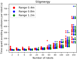
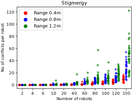
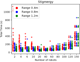
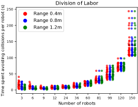
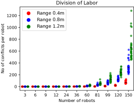
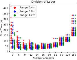
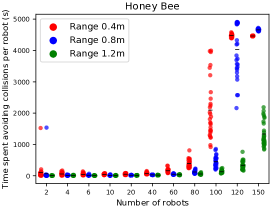
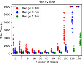
Figure 3: Congestion trends for scalability metrics for all three approaches. It would appear that the total time trends for all three approaches have a similar pattern for any decentralized system [3] and the optimal number of robots for our setting would be around $(N\in\ \{20-60\})$ roughly. All experiments of Stigmergy and Division of Labor converged to the superior quality opinion before 6000 s timeout period, whereas some experiments of $(N=120,\ R=0.8),(N=2,\ R=\{0.4,0.8\})$ and all experiments in $(N=120,\ R=0.4),(N=150,\ R=\{0.4,0.8\})$ for Honey Bee approach failed to converge to any opinion.

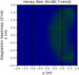
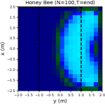
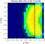
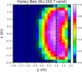
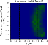
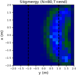
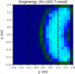
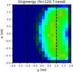
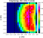
Figure 4: Stagnation heatmaps for the positive modulation approaches are shown in this figure for the combination $Z=A$, $R=0.4\ m$, $St_{T}$=1s (10 simulation timesteps). For the Honey bee approach $[T_{s},T_{f}]$ = $[95\%,\ 100\%]$ and Stigmergy approach $[T_{s},T_{f}]$ = $[85\%,\ 100\%]$. The barrier is of higher magnitude near the (zone A-Nest) boundary and has a decreasing radial gradient (in bands) away from zone A (the gradient follows a similar pattern to light intensity from the light centered at the end of zone A). Honey Bee approach is significantly more congested for a fixed combination compared to the Stigmergy approach (Honey Bee row is normalized by 5000 and Stigmergy row is normalized by 1000.)

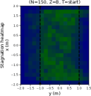
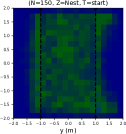
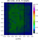
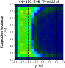
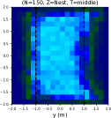
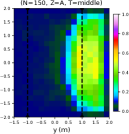
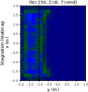
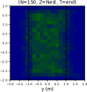
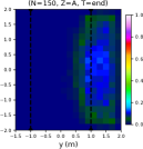
Figure 5: Stagnation heatmaps for Division of Labor approach is shown in this figure for $N=150$ $R=0.4\ m$, $St_{T}$=1s (10 simulation timesteps). T = start, represents $[T_{s},T_{f}]$ = $[0\%,\ 15\%]$, T = middle, represents $[T_{s},T_{f}]$ = $[15\%,\ 85\%]$, and T = end, represents $[T_{s},T_{f}]$ = $[85\%,\ 100\%]$. It can be seen that the magnitudes of stagnations are lesser compared to fig 4 and stagnations outside the assigned zones occur only in the starting phases of experiments. (All the rows are normalized by 1000.)

We investigate the scalability of the three approaches using the following metrics: 1. average time spent by every robot avoiding collisions with other robots and obstacles (arena walls), 2. average communication conflicts per robot while updating the virtual stigmergy, and 3. total time taken for all the robots to converge to highest quality opinion.

During all the experimental evaluations, we deploy the robots in a fixed arena dimension of $U=4\ m,\ V=4\ m$ and a Nest of size $2m\times 4m$ with site A quality $\rho_{A}=0.9$ and site B quality $\rho_{B}=0.1$. We varied the number of robots $N\in\{2,\ 4,\ 6,\ 10,\ 20,\ 40,\ 60,\ 80,\ 100,\ 120,\ 150\}$ corresponding to a Nest robot density of $\{1.3,\ 2.6,\ 3.9,\ 6.5,\ 13.1,\ 26.2,\ 39.4,\ 52.5,\ 65.7,\ 78.8,\ 98.5\}$ $\times$ $10^{-2}$ for Honey Bee and Stigmergy based decision-making strategies. Similarly, for Division of Labor technique, varied the robot numbers $N\in\{3,\ 6,\ 9,\ 12,\ 24,\ 36,\ 60,\ 81,\ 99,\ 120,\ 150\}$ corresponding to a Nest robot density of $\{1.9,\ 3.9,\ 5.9,\ 7.8,\ 15.7,\ 23.6,\ 39.4,\ 53.2,\ 65,\ 78.8,\ 98.5\}$ $\times$ $10^{-2}$. We set the communication range for all three techniques to $R\in\{0.4\ m,\ 0.8\ m,\ 1.2\ m\}$ and repeated each configuration 30 times with randomized robot placement following a normal distribution in the Nest zone.

To further understand the effects of the movement congestion, we plot the accumulated stagnation heatmap (defined as a robot spending over $St_{T}$ seconds in grids of size ($0.2\times 0.2$)) for an interval $[T_{s},T_{f}]$ in fig. 4 and fig. 5. The averaged movement change gridmap divides the arena into grids of size ($0.2\times 0.2$) for an interval $[T_{s},T_{f}]$ in fig. 6. Averaged movement change for each grid cell is calculated by averaging the movement vectors of robots in the grid over consecutive time steps ($x_{i}(t+1)-x_{i}(t)$). The stagnation heatmap and movement change gridmap are averaged over all 30 repetitions of a given configuration. The stagnation heatmap shows the congestion in space, while the averaged movement change gridmap shows the movement of robots.

Leveraging the metrics introduced above, we make the following inferences:

(1) Versioned local communication helps to overcome movement congestion, but doesn’t decongest the system. In fig. 3, the convergence time plot from the first two rows show that the Stigmergy and Division of Labor strategy converge significantly faster than the Honey Bee inspired, despite a comparable stagnation pattern in Stigmergy based (see fig. 4). The presence of stagnation with the Stigmergy approach indicates that congestion still exists. Faster convergence correlates with the lower time spent avoiding obstacles.

(2) Positive modulation in robot swarms increases the impact of stagnation and convergence time. A stagnation barrier (ref fig. 4) of increasing thickness with an increased number of robots occurs near the superior quality zone for Stigmergy and Honey Bee approaches. The barrier could result from positive modulation recruiting more and more robots to visit the higher quality zone as indicated in [7]. The barrier formation can also be inferred in fig. 6, where the averaged movement vectors of robots point towards each other, implying the robots’ intention to move towards each other. The formation of a barrier significantly hinders the information propagation in the Honey Bee approach, where belief propagation occurs through local broadcasts and the ability of robots to move to exchange beliefs effectively. The effect of the stagnation barrier is more pertinent for larger robot density and smaller communication range for Honey Bee inspired.

(3) Introducing structure through division of labor helps to minimize movement congestion. Fig. 5 shows the stagnation heatmap for the Division of Labor approach. The zone samplers and nest zone networker robots experience minimal stagnation within their respective zones as they are contained within their zones (except T=start, as robots are deployed in the Nest zone). The minimal stagnation in the grids directly reflects on the convergence time in fig. 3, where convergence time and time spent on collisions are minimal compared to the other two approaches. However, communication conflicts are larger than in the Stigmergy approach as more updates to the robot beliefs propagate through the swarm. The Stigmergy approach still suffers from movement congestion, thereby influencing the ability of the robots to move, sample, and update the stigmergy, which results in fewer conflicts.

(4) Longer communication ranges make a positive difference only with the local broadcast approach and make a negative impact with the versioned local communication strategy for a larger number of robots. Longer communication range combinations used in Honey Bee approach improve the total time and time spent avoiding collisions (ref fig. 3) compared to shorter communciation ranges ($R=0.4\ m<0.8\ m<1.2\ m$) for any number of robots in the system except ($N=150,\ R=\ 0.8\ m$, which has a slight increase in the time spent avoiding collisions per robots compared to $N=150,\ R=\ 0.4\ m$). Whereas the number of conflicts arising with the versioned local communication approach increases with a longer communication range and a higher number of robots ($N>60$). As the movement congestion doesn’t impact the propagation of beliefs with the versioned local communication approach, there is no significant improvement in the total time taken and time spent avoiding collisions for both these approaches compared to shorter communication ranges for a fixed number of robot combination (for $N>20$, ref fig 3).

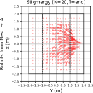
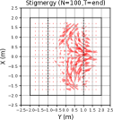
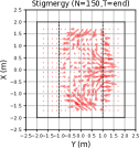
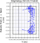
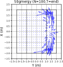
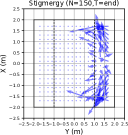
Figure 6: Movement changes for the combination $N\in\{20,\ 100,\ 150\}$, $R=0.4\ m$, $Z=A$, $[T_{s},T_{f}]$ = $[85\%,\ 100\%]$. The top row shows the averaged movement change of robots entering Zone A from Nest to sample (Zone A followers in Stigmergy approach fig. 2) and the bottom row shows the averaged movement change of robots entering Nest from Zone A (Nest followers in Stigmergy approach fig. 2.)

VI Conclusions

Current collective decision-making strategies rarely address congestion-related issues. This will have huge implications when it comes to deploying robot swarm systems in real-world scenarios, as these systems will scale poorly. In this paper, we discuss the impact of movement congestion and belief propagation conflicts on swarm behaviors, specifically collective decision-making. We find that using versioned local communication and Division of Labor mechanisms helps to reduce the impact of movement congestion, despite the increasing trends for communication conflicts. Further research could look into congestion-aware initialization strategies, congestion-aware collision avoidance, and dynamic approaches to switch between different state machines for collective decision-making systems. We believe our results transfer to other areas of swarm robotics such as foraging, task allocation, collective construction etc. and would welcome additional studies in these domains.

References

- [1] M. Brambilla, E. Ferrante, M. Birattari, and M. Dorigo, “Swarm robotics: a review from the swarm engineering perspective,” Swarm Intell, vol. 7, pp. 1–41, 2013.
- [2] M. Dorigo, G. Théraulaz, V. Trianni, and G. Theraulaz, “Reflections on the future of swarm robotics,” Science Robotics, vol. 2020, p. 4385. [Online]. Available: https://hal.science/hal-03362864
- [3] H. Hamann, “Superlinear scalability in parallel computing and multi-robot systems: Shared resources, collaboration, and network topology,” in Architecture of Computing Systems – ARCS 2018, M. Berekovic, R. Buchty, H. Hamann, D. Koch, and T. Pionteck, Eds. Cham: Springer International Publishing, 2018, pp. 31–42.
- [4] T. Seeley, “Honeybee democracy,” 12 2009.
- [5] N. Franks, S. Pratt, E. Mallon, N. Britton, and D. Sumpter, “Information flow, opinion polling and collective intelligence in house-hunting social insects,” Philosophical transactions of the Royal Society of London. Series B, Biological sciences, vol. 357, pp. 1567–83, 12 2002.
- [6] S. Garnier, J. Gautrais, and G. Theraulaz, “The biological principles of swarm intelligence,” Swarm Intell, vol. 1, pp. 3–31, 2007.
- [7] G. Valentini, H. Hamann, and M. Dorigo, “Self-organized collective decision making: The weighted voter model.” [Online]. Available: www.ifaamas.org
- [8] G. Valentini, E. Ferrante, H. Hamann, and M. Dorigo, “Collective decision with 100 kilobots: speed versus accuracy in binary discrimination problems collective decision with 100 kilo-bots: speed versus accuracy in binary discrimination problems. autonomous agents and multi-agent systems,” vol. 30, pp. 553–580, 2016. [Online]. Available: https://hal.archives-ouvertes.fr/hal-01403730
- [9] J. Prasetyo, G. De Masi, and E. Ferrante, “Collective decision making in dynamic environments,” Swarm Intelligence, vol. 13, 12 2019.
- [10] G. Valentini, D. Brambilla, H. Hamann, and M. Dorigo, “Collective perception of environmental features in a robot swarm,” in Swarm Intelligence, M. Dorigo, M. Birattari, X. Li, M. López-Ibáñez, K. Ohkura, C. Pinciroli, and T. Stützle, Eds. Cham: Springer International Publishing, 2016, pp. 65–76.
- [11] K. Chin, Y. Khaluf, and C. Pinciroli, “Minimalistic collective perception with imperfect sensors,” 09 2022.
- [12] J. T. Ebert, M. Gauci, and R. Nagpal, “Multi-feature collective decision making in robot swarms,” in Adaptive Agents and Multi-Agent Systems, 2018.
- [13] J. T. Ebert, M. Gauci, F. Mallmann-Trenn, and R. Nagpal, “Bayes bots: Collective bayesian decision-making in decentralized robot swarms.”
- [14] Q. Shan and S. Mostaghim, “Discrete collective estimation in swarm robotics with distributed bayesian belief sharing,” Swarm Intelligence, vol. 15, 12 2021.
- [15] K. Pfister and H. Hamann, “Collective decision-making with bayesian robots in dynamic environments,” in 2022 IEEE/RSJ International Conference on Intelligent Robots and Systems (IROS), 2022, pp. 7245–7250.
- [16] M. Raoufi, H. Hamann, and P. Romanczuk, “Speed-vs-accuracy tradeoff in collective estimation: An adaptive exploration-exploitation case,” in 2021 International Symposium on Multi-Robot and Multi-Agent Systems (MRS), 2021, pp. 47–55.
- [17] Y. Khaluf, “Edge detection in static and dynamic environments using robot swarms,” 09 2017, pp. 81–90.
- [18] Y. Khaluf, M. Allwright, I. Rausch, P. Simoens, and M. Dorigo, “Construction task allocation through the collective perception of a dynamic environment,” 11 2020.
- [19] I. D. Couzin and N. R. Franks, “Self-organized lane formation and optimized traffic flow in army ants.”
- [20] D. Helbing, P. Molnár, I. J. Farkas, and K. Bolay, “Self-organizing pedestrian movement,” https://doi.org/10.1068/b2697, vol. 28, pp. 361–383, 6 2001. [Online]. Available: https://journals.sagepub.com/doi/10.1068/b2697
- [21] A. Editors, J. Hu, Z. Peng, Y. T. dos Passos, X. Duquesne, and L. S. Marcolino, “On the throughput of the common target area for robotic swarm strategies,” 2022. [Online]. Available: https://doi.org/10.3390/math10142482
- [22] G. Yu and M. Wolf, “Congestion prediction for large fleets of mobile robots,” in ICRA 2023, 2023. [Online]. Available: https://www.amazon.science/publications/congestion-prediction-for-large-fleets-of-mobile-robots
- [23] L. Soriano Marcolino and L. Chaimowicz, “Traffic control for a swarm of robots: Avoiding group conflicts,” 11 2009, pp. 1949 – 1954.
- [24] F. Wu, V. S. Varadharajan, and G. Beltrame, “Collision-aware task assignment for multi-robot systems,” in 2019 International Symposium on Multi-Robot and Multi-Agent Systems (MRS), 2019, pp. 30–36.
- [25] M. Barciś and H. Hellwagner, “Information distribution in multi-robot systems: Adapting to varying communication conditions,” in 2021 Wireless Days (WD), 2021, pp. 1–8.
- [26] P. Rybski, S. Stoeter, M. Gini, D. Hougen, and N. Papanikolopoulos, “Performance of a distributed robotic system using shared communications channels,” Robotics and Automation, IEEE Transactions on, vol. 18, pp. 713 – 727, 11 2002.
- [27] M. Bettini, A. Shankar, and A. Prorok, “Heterogeneous multi-robot reinforcement learning,” 2023.
- [28] E. Ferrante, A. E. Turgut, E. A. Duéñez-Guzmán, M. Dorigo, and T. Wenseleers, “Evolution of self-organized task specialization in robot swarms,” PLoS Computational Biology, vol. 11, 2015.
- [29] N. Ayanian, “Dart: Diversity-enhanced autonomy in robot teams,” The International Journal of Robotics Research, vol. 38, no. 12-13, pp. 1329–1337, 2019. [Online]. Available: https://doi.org/10.1177/0278364919839137
- [30] A. Ozdemir, M. Gauci, and R. Groß, “Shepherding with robots that do not compute,” 09 2017.
- [31] V. S. Varadharajan, D. St-Onge, B. Adams, and G. Beltrame, “Swarm relays: distributed self-healing ground-and-air connectivity chains,” IEEE Robotics and Automation Letters, vol. 5, no. 4, pp. 5347–5354, 2020.
- [32] P.-Y. Lajoie and G. Beltrame, “Swarm-slam : Sparse decentralized collaborative simultaneous localization and mapping framework for multi-robot systems,” 2023.
- [33] I. D. Miller, F. Cladera, T. Smith, C. J. Taylor, and V. Kumar, “Stronger together: Air-ground robotic collaboration using semantics,” IEEE Robotics and Automation Letters, vol. 7, no. 4, pp. 9643–9650, 2022.
- [34] M. Dorigo, D. Floreano, L. M. Gambardella, F. Mondada, S. Nolfi, T. Baaboura, M. Birattari, M. Bonani, M. Brambilla, A. Brutschy, D. Burnier, A. Campo, A. L. Christensen, A. Decugniere, G. Di Caro, F. Ducatelle, E. Ferrante, A. Forster, J. M. Gonzales, J. Guzzi, V. Longchamp, S. Magnenat, N. Mathews, M. Montes de Oca, R. O’Grady, C. Pinciroli, G. Pini, P. Retornaz, J. Roberts, V. Sperati, T. Stirling, A. Stranieri, T. Stutzle, V. Trianni, E. Tuci, A. E. Turgut, and F. Vaussard, “Swarmanoid: A novel concept for the study of heterogeneous robotic swarms,” IEEE Robotics Automation Magazine, vol. 20, no. 4, pp. 60-71, 2013.
- [35] M. Saska, V. Vonásek, T. Krajník, and L. Preucil, “Coordination and navigation of heterogeneous mav–ugv formations localized by a ‘hawk-eye’-like approach under a model predictive control scheme,” The International Journal of Robotics Research, vol. 33, pp. 1393 – 1412, 2014.
- [36] C. Pinciroli, A. Lee-Brown, and G. Beltrame, “A tuple space for data sharing in robot swarms,” in 9th EAI International Conference on Bio-inspired Information and Communications Technologies (BICT 2015). European Union Digital Library, May 2016. [Online]. Available: https://publications.polymtl.ca/4727/