Interferometric single-pixel imaging with a multicore fiber

Abstract

Lensless illumination single-pixel imaging with a multicore fiber (MCF) is a computational imaging technique that enables potential endoscopic observations of biological samples at cellular scale. In this work, we show that this technique is tantamount to collecting multiple symmetric rank-one projections (SROP) of a Hermitian interferometric matrix—a matrix encoding the spectral content of the sample image. In this model, each SROP is induced by the complex sketching vector shaping the incident light wavefront with a spatial light modulator (SLM), while the projected interferometric matrix collects up to $O(Q^{2})$ image frequencies for a $Q$-core MCF. While this scheme subsumes previous sensing modalities, such as raster scanning (RS) imaging with beamformed illumination, we demonstrate that collecting the measurements of $M$ random SLM configurations—and thus acquiring $M$ SROPs—allows us to estimate an image of interest if $M$ and $Q$ scale linearly (up to log factors) with the image sparsity level, hence requiring much fewer observations than RS imaging or a complete Nyquist sampling of the $Q\times Q$ interferometric matrix. This demonstration is achieved both theoretically, with a specific restricted isometry analysis of the sensing scheme, and with extensive Monte Carlo experiments. Experimental results made on an actual MCF system finally demonstrate the effectiveness of this imaging procedure on a benchmark image.

1 Introduction

Recently, the imaging community became more and more interested in lensless solutions, providing opportunities to design imaging systems free from the constraints imposed by traditional camera architectures. Cheaper, lighter, and enabling compressive imaging with large field-of-view (FOV), Lensless Imaging (LI) is convenient for medical applications such as microscopy [1, 2] and in vivo imaging [3, 4] where the extreme miniaturization of the imaging probe (diameter $\leq$ 200 $\mu$m) offers a minimally invasive route to image at depths unreachable in microscopy [5]. Paving the way for deep biological tissues [6] and brain imaging with the capability to produce focal planes at various distances from the fiber tip, intensive research effort emerged for Lensless Endoscopy (LE) using multimode fibers [7, 8, 9, 10] or MultiCore Fibers (MCF) [11, 12, 13].

In the field of Computational Imaging (CI) to which LI belongs, a mathematical model is required to describe the observations as a function of the object to be imaged. Regarding the efficiency aspects, two categories of requirement must be considered when developping CI applications; (i) the model must be physically reliable but also computationnally efficient to speed up the reconstruction algorithms (ii) the acquisition method must minimize the number of observations (also called sample complexity) needed to accurately estimate the object of interest while remaining fast. In single-pixel MCF-LI, Speckle Imaging (SI) consists in randomly shaping the wavefront of the light input to the (weakly coupled) cores entering the MCF to illuminate the entire object with a randomly distributed intensity. The fraction of the light re-emitted (either at other wavelengths by fluorescence or by simple reflection) is integrated in a single-pixel sensor, playing the role of a complete projection of the speckle on the object. Compared to Raster Scanning (RS) the object with a translating focused spot [11], SI has been shown to reduce the sample complexity [14].

In this work, we push a leap forward towards real-time compressive LE, keeping the low sample complexity enabled by SI and introducing light propagation physics in the forward model of MCF imaging using a wavefront-shaping device. We point out that inserting the physics yields an interferometric sensing model similar to radio-inteferometry applications [15, 16], where the interferences of the light emmited by the cores composing the MCF give specific access to the Fourier content of the object to be imaged. The sampling complexity of the underlying model is analyzed both theoretically and experimentally.

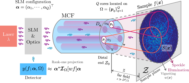
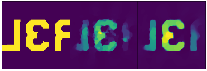
Figure 1: (top) Interferometric LI and its link with ROPs of the interferometric matrix. (bottom) left: ground truth, center: reconstruction with ($Q$,$M$)=(110,49), right: reconstruction with ($Q$,$M$)=(110,$2\cdot 10^{4}$).

2 Sensing model

Considering an MCF with diameter $D$ and $Q$ fiber cores (see Fig. 1-top) whose locations on the MCF distal end $\mathcal{Z}_{0}$ are in $\Omega:=\{\boldsymbol{p}_{q}\}_{q=1}^{Q}\subset\mathbb{R}^{2}$, and assuming a planar sample in the plane $\mathcal{Z}$ at a distance $z$ from $\mathcal{Z}_{0}$, by optically shaping the light wavefront with an SLM, we can set to $\alpha_{q}\in\mathbb{C}$ the complex amplitude of the electromagnetic field at each fiber core $\boldsymbol{p}_{q}$. Writing $\boldsymbol{\alpha}=(\alpha_{1},\ldots,\alpha_{Q})^{\top}\in\mathbb{C}^{Q}$ and $\boldsymbol{x}\in\mathbb{R}^{2}$ a point on $\mathcal{Z}$, under the far-field approximation $z\gg D^{2}/\lambda$ (with $\lambda$ the laser wavelength) the illumination produced by the MCF on $\mathcal{Z}$ reads [14]

$$\textstyle S(\boldsymbol{x};\boldsymbol{\alpha})\approx w(\boldsymbol{x})\,\big{|}\!\sum_{q=1}^{Q}\alpha_{q}e^{\frac{2\pi\mathrm{i}\mkern 1.0mu}{\lambda z}\boldsymbol{p}_{q}^{\top}\boldsymbol{x}}\big{|}^{2},$$

where $w$ is a smooth vignetting function—a Gaussian envelope with a diameter inversely proportional to the fiber cores diameter—determining the FOV. In RS mode, a focused beam can be obtained in $\mathcal{Z}$ when the $Q$ fiber core locations in $\Omega$ are arranged in a Fermat’s golden spiral shape [17]; we will restrict our analysis to this configuration. The LE collects a fraction $c\in(0,1)$ of the light $y$ globally re-emitted by the sample—as modeled by the fluorophore density map $f(\boldsymbol{x})$—under the illumination $S$. For short time exposure and low intensity illumination, fluorescence theory provides (in a noiseless regime)

$$y(f;\boldsymbol{\alpha},\Omega)=c\int_{\mathbb{R}^{2}}S(\boldsymbol{x};\boldsymbol{\alpha})f(\boldsymbol{x})\mathrm{d}\boldsymbol{x}$$

$$=c\sum_{j,k=1}^{Q}\alpha_{j}^{*}\alpha_{k}\int_{\mathbb{R}^{2}}e^{\frac{2\pi\mathrm{i}\mkern 1.0mu}{\lambda z}(\boldsymbol{p}_{k}-\boldsymbol{p}_{j})^{\top}\boldsymbol{x}}w(\boldsymbol{x})f(\boldsymbol{x})\mathrm{d}\boldsymbol{x}\in\mathbb{R}_{+},$$

with the number of collected photons $y$ being Poisson distributed. Therefore, introducing the interferometry matrix $\boldsymbol{\mathcal{I}}_{\Omega}[g]\in\mathbb{C}^{Q\times Q}$ such that, for a function $g:\mathbb{R}^{2}\to\mathbb{R}$, $(\boldsymbol{\mathcal{I}}_{\Omega}[g])_{jk}:=\int_{\mathbb{R}^{2}}e^{\frac{2\pi\mathrm{i}\mkern 1.0mu}{\lambda z}(\boldsymbol{p}_{k}-\boldsymbol{p}_{j})^{\top}\boldsymbol{x}}g(\boldsymbol{x})\mathrm{d}\boldsymbol{x}$ with $\boldsymbol{\mathcal{I}}_{\Omega}[g]$ Hermitian, assuming $c=1$ and considering the scenario where we collect $M$ LE observations $\boldsymbol{y}=(y_{1},\ldots,y_{M})^{\top}$, each associated with a specific $\boldsymbol{\alpha}_{m}$ for $1\leqslant m\leqslant M$,

$$y(f;\boldsymbol{\alpha}_{m},\Omega)=\boldsymbol{\alpha}_{m}^{*}\,\boldsymbol{\mathcal{I}}_{\Omega}[f^{\circ}\,]\,\boldsymbol{\alpha}_{m}=\big{\langle}\boldsymbol{\alpha}_{m}\boldsymbol{\alpha}_{m}^{*},\boldsymbol{\mathcal{I}}_{\Omega}\big{[}f^{\circ}\,\big{]}\big{\rangle}_{F},$$

with $f^{\circ}:=wf$ is the image $f$ vignetted by $w$. Under a high photon counting regime, and gathering all possible noise sources in an additive term $\boldsymbol{n}$, we can thus compactly write the SI sensing as

$$\begin{split}\boldsymbol{y}=\boldsymbol{\mathcal{A}}\circ\boldsymbol{\mathcal{I}}_{\Omega}\big{[}f^{\circ}\,\big{]}+\boldsymbol{n},\leavevmode\nobreak\ &\text{with}(\mathcal{A}[\boldsymbol{H}])_{m}:=\boldsymbol{\alpha}_{m}^{*}\boldsymbol{H\alpha}_{m},\\ &\text{for}\ \boldsymbol{H}=\boldsymbol{H}^{*}\ \text{and}\ 1\leqslant m\leqslant M.\end{split}$$ (1)

We thus observe that (1) is tantamount to first sampling the Fourier transform of $f^{\circ}$ over frequencies selected in the difference set $\mathcal{V}:=\frac{2\pi}{\lambda z}(\Omega-\Omega)=\{\frac{2\pi}{\lambda z}(\boldsymbol{p}_{j}-\boldsymbol{p}_{k})\}_{j,k=1}^{Q}$, and next performing $M$ symmetric rank-one projections (SROP [18, 19]) of $\boldsymbol{\mathcal{I}}_{\Omega}[f^{\circ}\,]$ as determined by $\mathcal{A}$ and the complex amplitude vectors $\{\boldsymbol{\alpha}_{m}\}_{m=1}^{M}$. Thus, the SI sensing corresponds to a specific interferometric system: assuming we collect enough SROP observations, we can potentially estimate the interferometry matrix $\boldsymbol{\mathcal{I}}_{\Omega}[f^{\circ}\,]$. The system is thus equivalent to the radio-interferometry principles [16]—each fiber core playing somehow the role of a radio telescope and each entry of $(\boldsymbol{\mathcal{I}}_{\Omega}[f^{\circ}\,])_{jk}$ probing the frequency content of $f^{\circ}$ on the “visibility” $\nu_{jk}:=\frac{2\pi}{\lambda z}(\boldsymbol{p}_{j}-\boldsymbol{p}_{k})$.

3 Interferometric structural models

If one aims to image a vignetted sample that is $K$-sparse in the spatial domain, i.e., it is composed of a few spikes as $f^{\circ}(\boldsymbol{x})=\sum_{i=1}^{K}\rho_{i}\delta(\boldsymbol{x}-\boldsymbol{x}_{i})$ for $K\ll Q$, the entry "$jk$" of the interferometric matrix reads $\boldsymbol{\mathcal{I}}_{\Omega}\big{[}f^{\circ}\big{]}_{jk}=\sum_{i=1}^{K}\rho_{i}e^{\mathrm{i}\mkern 1.0mu2\pi(\boldsymbol{p}_{k}-\boldsymbol{p}_{j})^{\top}\boldsymbol{x}_{i}}.$ We can therefore write the interferometric matrix as

$$\boldsymbol{\mathcal{I}}_{\Omega}\big{[}f^{\circ}\big{]}=\sum_{i}\rho_{i}\boldsymbol{u}(\boldsymbol{x}_{i})\boldsymbol{u}^{*}(\boldsymbol{x}_{i}),\leavevmode\nobreak\ \leavevmode\nobreak\ \leavevmode\nobreak\ \leavevmode\nobreak\ \boldsymbol{u}(\boldsymbol{x})_{j}:=e^{-\mathrm{i}\mkern 1.0mu2\pi\boldsymbol{p}_{j}^{\top}\boldsymbol{x}},$$

which shows that it is low-rank with rank $K$. More generally, for a sample $f^{\circ}$ that can be assumed sparsely represented in a collection of functions $\{\psi_{k}\}_{k=1}^{d}$ (e.g., a wavelet basis for bandlimited function supported inside $\Omega$), i.e., $f^{\circ}(\boldsymbol{x})=\sum_{k=1}^{d}\rho_{k}\psi_{k}(\boldsymbol{x})$ with $\lVert\boldsymbol{\rho}\rVert_{0}=K\ll d$, then the interferometric matrix belongs to a subspace of dimension $K$ and writes as $\boldsymbol{\mathcal{I}}_{\Omega}[f^{\circ}]=\sum_{k|\rho_{k}\neq 0}^{K}\rho_{k}\boldsymbol{\mathcal{I}}_{\Omega}[\psi_{k}]$.

4 Image reconstruction

Assuming the sample $f^{\circ}\in\Omega$ is band-limited, we are interested in accurately estimating a discretisation $\boldsymbol{f}\in\mathbb{R}^{N}$ of $f^{\circ}$ We consider a discretisation of (1) that reads

$$\boldsymbol{y}=\boldsymbol{\mathcal{A}}\circ\tilde{\boldsymbol{\mathcal{I}}}_{\Omega}[\boldsymbol{f}]+\boldsymbol{n},\text{with }\tilde{\boldsymbol{\mathcal{I}}}_{\Omega}[\boldsymbol{f}]=\boldsymbol{R}_{\tilde{\mathcal{V}}}\boldsymbol{F}\boldsymbol{f},$$

where $\boldsymbol{F}$ is the Fourier matrix and $\boldsymbol{R}_{\tilde{\mathcal{V}}}:\mathbb{C}^{N}\mapsto\mathbb{C}^{Q\times Q}$ is the restriction to the set $\tilde{\mathcal{V}}$ obtained as a Cartesian gridding of the (off-grid) difference set $\mathcal{V}$ (reached by nearest neighbors). From the factorization of this model, we first conclude that the set $\tilde{\mathcal{V}}$ should ideally be composed of as many distinct frequencies as possible (except for the zero frequency that has multiplicity $Q$) to improve our knowledge of $\boldsymbol{f}$. Interestingly, we can show numerically that Fermat’s gold spiral arrangement ensures the unicity of the visibilities $\tilde{\nu}_{jk}$ when $j\neq k$, i.e., $\tilde{\mathcal{V}}$ is composed of $Q(Q-1)+1$ distinct frequencies. In a noiseless scenario, we have shown that there exists a combination of $M_{0}=O(Q^{2})$ deterministic ROP observations that exactly recovers $\tilde{\boldsymbol{\mathcal{I}}}_{\Omega}[f^{\circ}\,]$. Therefore, in a compressive setting, we could first leverage the low-complexity structure of $\tilde{\boldsymbol{\mathcal{I}}}_{\Omega}[f^{\circ}\,]$—as induced from that of $\boldsymbol{f}$—to recover $\tilde{\boldsymbol{\mathcal{I}}}_{\Omega}[\boldsymbol{f}]$ from $M<M_{0}$ random complex ROPs, and then infer $\boldsymbol{f}$ from its $Q(Q-1)+1$ frequencies encoded in $\tilde{\boldsymbol{\mathcal{I}}}_{\Omega}[\boldsymbol{f}]$, this second step being similar to the inverse problem posed in radio-interferometry [16, 15]. In a simpler case where the cores are placed at all integer positions, the interferometric matrix is shown to be circulant and low-rank, i.e., $\tilde{\boldsymbol{\mathcal{I}}}_{\Omega}[\boldsymbol{f}]=\mathcal{T}\circ\boldsymbol{F}\boldsymbol{f}$ where $\mathcal{T}:\mathbb{C}^{N}\mapsto\mathbb{C}^{N\times N}$ is the operator that turns a vector into a circulant matrix. In this situation, the sensing operator $\mathcal{B}$ respects a specific RIP-$\ell_{2}/\ell_{1}$ property over the set of sparse images—thus extending former approaches restricted to real sparse and low-rank matrices [18], and the RIP of random partial Fourier sensing characterized by $\tilde{\mathcal{V}}$ [20]. Proposition 4.1 shows that proving this RIP-$\ell_{2}/\ell_{1}$ for $\mathcal{B}$ implies we can reliably estimate it in a single basis pursuit denoising program (BPDN) with an $\ell_{1}$ fidelity term. This happens with high probability if the vectors $\{\boldsymbol{\alpha}_{m}\}_{m=1}^{M}$ are random and sub-Gaussian, and both $M$ and $Q^{2}$ are large compared to the sparsity level of $\boldsymbol{f}$.

Proposition 4.1 ($\ell_{2}/\ell_{1}$ instance optimality of BPDN${}_{\ell_{1}}$).

Let $\boldsymbol{\mathcal{B}}:=\boldsymbol{\mathcal{A}}\circ\mathcal{T}\circ\boldsymbol{F}$ be an operator that respects the $\text{RIP}_{\ell_{2}/\ell_{1}}(k,\alpha_{k},\beta_{k})$ for $k\in\{K,K+K^{\prime}\}$ with $K^{\prime}>2K$, and ${\textstyle\frac{1}{\sqrt{2}}}m_{K+K^{\prime}}-M_{K^{\prime}}\frac{\sqrt{K}}{\sqrt{K^{\prime}}}\geqslant\gamma>0$, for some $M_{K^{\prime}}>0$. Then, $\forall\boldsymbol{f}\in\mathbb{R}^{N}$ , the estimate

$$\hat{\boldsymbol{f}}\in\operatorname*{arg\,min}_{\boldsymbol{u}}\leavevmode\nobreak\ \lVert\boldsymbol{u}\rVert_{1}\leavevmode\nobreak\ \leavevmode\nobreak\ \mathrm{s.\!t.}\big{\lVert}\underbrace{\boldsymbol{\mathcal{B}}(\boldsymbol{f})+\boldsymbol{n}}_{\boldsymbol{y}}-\boldsymbol{\mathcal{B}}(\boldsymbol{u})\big{\rVert}_{1}\leqslant\epsilon\vspace*{-0.4cm}$$

satisfies

$$\lVert\boldsymbol{f}-\hat{\boldsymbol{f}}\rVert_{2}\leqslant C\frac{\lVert\boldsymbol{f}-\boldsymbol{f}_{K}\rVert_{1}}{\sqrt{K}}+D\frac{\epsilon}{m}$$

The current theoretical derivations are accompanied by numerical (not shown in this abstract) and experimental reconstruction results (see lead-in in Fig. 1-bottom) that suggest Proposition 4.1 may also hold when relaxing the cited assumptions. Additionnally, this may extend to other optimisation problems like LASSO [21] or lagrangian formulations with various regularization terms ($\ell_{1}$ in the identity or orthonormal basis, total variation).

References

- [1] Aydogan Ozcan and Utkan Demirci. Ultra wide-field lens-free monitoring of cells on-chip. Lab Chip, 8:98–106, 2008.
- [2] Aydogan Ozcan and Euan McLeod. Lensless imaging and sensing. Annual Review of Biomedical Engineering, 18(1):77–102, 2016. PMID: 27420569.
- [3] Grace Kuo, Fanglin Linda Liu, Irene Grossrubatscher, Ren Ng, and Laura Waller. On-chip fluorescence microscopy with a random microlens diffuser. Opt. Express, 28(6):8384–8399, Mar 2020.
- [4] Jesse K. Adams, Vivek Boominathan, Sibo Gao, Alex V. Rodriguez, Dong Yan, Caleb Kemere, Ashok Veeraraghavan, and Jacob T. Robinson. In vivo fluorescence imaging with a flat, lensless microscope. bioRxiv, 2020.
- [5] Vivek Boominathan, Jesse K. Adams, M. Salman Asif, Benjamin W. Avants, Jacob T. Robinson, Richard G. Baraniuk, Aswin C. Sankaranarayanan, and Ashok Veeraraghavan. Lensless Imaging: A computational renaissance. IEEE Signal Processing Magazine, 33(5):23–35, 2016.
- [6] W. Choi, M. Kang, and J.H. et al. Hong. Flexible-type ultrathin holographic endoscope for microscopic imaging of unstained biological tissues. Nature Communications, 4469(13), 2022.
- [7] D. Septier, V. Mytskaniuk, R. Habert, D. Labat, K. Baudelle, A. Cassez, G. Brévalle-Wasilewski, M. Conforti, G. Bouwmans, H. Rigneault, and A. Kudlinski. Label-free highly multimodal nonlinear endoscope. Opt. Express, 30(14):25020–25033, Jul 2022.
- [8] Benjamin Lochocki, Max V. Verweg, Jeroen J. M. Hoozemans, Johannes F. de Boer, and Lyubov V. Amitonova. Epi-fluorescence imaging of the human brain through a multimode fiber. APL Photonics, (7), 2022.
- [9] Demetri Psaltis and Christophe Moser. Imaging with Multimode Fibers. Optics and Photonics News, 27(1):24—-31, 2016.
- [10] Tomas Cizmar and Kishan Dholakia. Exploiting multimode waveguides for pure fibre-based imaging. Nature Communications, 3(May), 2012.
- [11] Siddharth Sivankutty, Viktor Tsvirkun, Géraud Bouwmans, Dani Kogan, Dan Oron, Esben Ravn Andresen, and Hervé Rigneault. Extended field-of-view in a lensless endoscope using an aperiodic multicore fiber. Optics Letters, 41(15):3531, 2016.
- [12] Esben Ravn Andresen, Siddharth Sivankutty, Viktor Tsvirkun, Géraud Bouwmans, and Hervé Rigneault. Ultrathin endoscopes based on multicore fibers and adaptive optics: status and perspectives. Journal of Biomedical Optics, 21(12):121506, 2016.
- [13] Debaditya Choudhury, Duncan K. McNicholl, Audrey Repetti, Itandehui Gris-Sánchez, Tim A. Birks, Yves Wiaux, and Robert R. Thomson. Compressive optical imaging with a photonic lantern. 2019.
- [14] Stéphanie Guérit, Siddharth Sivankutty, John Lee, Hervé Rigneault, and Laurent Jacques. Compressive imaging through optical fiber with partial speckle scanning. SIAM Journal on Imaging Sciences, 15(2):387–423, 2022.
- [15] R. E. Carrillo, J. D. McEwen, and Y. Wiaux. Sparsity Averaging Reweighted Analysis (SARA): A novel algorithm for radio-interferometric imaging. Monthly Notices of the Royal Astronomical Society, 426(2):1223–1234, 2012.
- [16] Yves Wiaux, Laurent Jacques, Gilles Puy, Anna MM Scaife, and Pierre Vandergheynst. Compressed sensing imaging techniques for radio interferometry. Monthly Notices of the Royal Astronomical Society, 395(3):1733–1742, 2009.
- [17] Siddharth Sivankutty, Viktor Tsvirkun, Olivier Vanvincq, Géraud Bouwmans, Esben Ravn Andresen, and Hervé Rigneault. Nonlinear imaging through a Fermat’s golden spiral multicore fiber. Optics Letters, 43(15):3638, 2018.
- [18] Yuxin Chen, Yuejie Chi, and Andrea J Goldsmith. Exact and stable covariance estimation from quadratic sampling via convex programming. IEEE Transactions on Information Theory, 61(7):4034–4059, 2015.
- [19] T Tony Cai, Anru Zhang, et al. Rop: Matrix recovery via rank-one projections. Annals of Statistics, 43(1):102–138, 2015.
- [20] Simon Foucart and Holger Rauhut. A mathematical introduction to compressive sensing. Bull. Am. Math, 54(2017):151–165, 2017.
- [21] D. E.N. Van Ewout Berg and Michael P. Friedlander. Probing the pareto frontier for basis pursuit solutions. SIAM Journal on Scientific Computing, 31(2):890–912, 2008.