Efficient and Accurate Optimal Transport with
Mirror Descent and Conjugate Gradients

Abstract

We design a novel algorithm for optimal transport by drawing from the entropic optimal transport, mirror descent and conjugate gradients literatures. Our scalable and GPU parallelizable algorithm is able to compute the Wasserstein distance with extreme precision, reaching relative error rates of $10^{-8}$ without numerical stability issues. Empirically, the algorithm converges to high precision solutions more quickly in terms of wall-clock time than a variety of algorithms including log-domain stabilized Sinkhorn’s Algorithm. We provide careful ablations with respect to algorithm and problem parameters, and present benchmarking over upsampled MNIST images, comparing to various recent algorithms over high-dimensional problems. The results suggest that our algorithm can be a useful addition to the practitioner’s optimal transport toolkit.

1 INTRODUCTION

Whenever one requires a metric-aware statistical distance given an event space equipped with a metric, optimal transport (OT) distances such as the Wasserstein metric provide an intuitive recipe with desirable theoretical properties. Consequently, fast, scalable and accurate computation of OT distances is a major problem encountered in various scientific fields. Examples include point cloud registration (Shen et al., 2021), color transfer (Pitie et al., 2005; Ferradans et al., 2014; Rabin et al., 2014), shape matching (Feydy et al., 2017), texture mixing (Ferradans et al., 2013; Bonneel et al., 2015) and meshing (Digne et al., 2014) in computer vision and graphics, quantum mechanics (Léonard, 2012), astronomy (Frisch et al., 2002; Levy et al., 2021) and quantum chemistry (Bokanowski & Grébert, 1996) in physics, and generative modelling (Gulrajani et al., 2017; Genevay et al., 2018), reinforcement learning (Ferns et al., 2004; Dadashi et al., 2021) and neural architecture search (Kandasamy et al., 2018) in machine learning. While significant progress was made on fast OT solvers with the introduction of Sinkhorn’s Algorithm (SA) to the world of GPUs (Sinkhorn & Knopp, 1967; Sinkhorn, 1967; Cuturi, 2013), this efficiency comes at the cost of a poor trade-off between speed and precision. As we show, issues posed by this trade-off are especially apparent when dealing with high-entropy marginals. Although various sophisticated new algorithms have favourable theoretical convergence properties over SA, they are rarely as GPU-friendly and easy-to-implement such that SA still remains a serious baseline in practice (Flamary et al., 2021; Lin et al., 2022). In this work, we set out to design a flexible algorithm that shares similar characteristics (e.g., parallelizability, scalability) to SA, but can rapidly compute precise solutions.

Contributions.

Our first contribution is to formally define and study the generalization of SA as a mirror descent (MD) procedure with approximate Bregman projections. Namely, we show that typical $\varepsilon$-scaling (or simulated annealing) algorithms as in Schmitzer (2019) can be understood as an MD procedure, where a sequence of Bregman projection problems (onto the transportation polytope) are initialized with a particular warm-starting heuristic and solved approximately. Then, we propose a better warm-starting heuristic and show its efficiency gains empirically. Our second contribution is a novel instantiation of the conjugate gradients (CG) method as an alternative to SA (and similar algorithms) for Bregman projections in OT. Coupled with the MD approach and an efficient, easy-to-implement line search procedure that we develop, they provide a viable alternative to readily accessible OT solvers, especially when high-precision solutions are required for high-dimensional problems.

2 BACKGROUND

Here, we present our notation, basics of OT and the necessary background on MD and CG for our approach (see Appx. A for an extended version of this section).

Notation and Definitions.

In this work, we consider discrete OT, where the event space ${\mathcal{X}}$ is finite with $n$ elements and ${\Delta_{n}\subset\mathbb{R}_{\geq 0}^{n}}$ is the $(n{-}1)$-simplex. The row sum of an ${n\times n}$ matrix $P$ is given by ${\bm{r}}(P)$ and the column sum by ${\bm{c}}(P)$. Given target marginals ${{\bm{r}},{\bm{c}}\in\Delta_{n}}$, the transportation polytope is written as ${{\mathcal{U}}({\bm{r}},{\bm{c}})=\{P\in\mathbb{R}^{n\times n}_{\geq 0}~{}|~{}{\bm{r}}(P)={\bm{r}},{\bm{c}}(P)={\bm{c}}\}}$. Throughout, we assume all entries of ${\bm{r}},{\bm{c}}$ are positive. Division, $\exp$ and $\log$ over vectors or matrices indicate element-wise operations. For elementwise multiplication, we use the symbol $\odot$. Vectors in $\mathbb{R}^{n}$ are taken to be column vectors and concatenation of two column vectors ${\bm{x}},{\bm{y}}$ is $({\bm{x}},{\bm{y}})$. Matrix and vector inner products alike are given by $\langle\cdot,\cdot\rangle$. An ${n\times n}$ diagonal matrix with ${\bm{x}}\in\mathbb{R}^{n}$ along the diagonal is written as $\mathbf{D}({\bm{x}})$.

2.1 Optimal Transport

Given a cost matrix ${C\in{[0,1]}^{n\times n}}$, where $C_{ij}$ is the transportation cost between ${{\bm{x}}_{i},{\bm{x}}_{j}\in{\mathcal{X}}}$, we study the OT problem given by the following linear program: [2] P ∈U(r, c)⟨P, C ⟩. Entropic regularization of (2.1) is often used for efficient computation on GPUs (Cuturi, 2013): [2] P ∈U(r, c)⟨P, C ⟩- 1γH(P), where $\gamma>0$ and ${H(P)=-\sum_{ij}P_{ij}\log P_{ij}}$ is the Shannon entropy of the joint distribution $P$. The Lagrangian of (2.1) is strictly convex in $P$ so that a unique solution with respect to $P\in{\mathcal{U}}({\bm{r}},{\bm{c}})$ exists:

$$P_{ij}({\bm{u}},{\bm{v}})=\exp\{u_{i}+v_{j}-\gamma C_{ij}\}.$$ (1)

Finding optimal ${{\bm{u}},{\bm{v}}\in\mathbb{R}^{n}}$ reduces to the following unconstrained dual problem (Bregman projection): [2] u, v∈R^ng(u, v) = ∑_ij P_ij(u, v) - ⟨u, r⟩- ⟨v, c⟩.

The SA algorithm can be used to solve (2.1) and approximately project $\exp{\{-\gamma C\}}$ onto ${\mathcal{U}}({\bm{r}},{\bm{c}})$ given some stopping criterion. Sinkhorn updates are guaranteed to converge to dual-optimal values as the number of iterations $k\rightarrow\infty$ (Sinkhorn & Knopp, 1967; Sinkhorn, 1967; Franklin & Lorenz, 1989; Knight, 2008). Later, SA was shown to converge with complexity $\widetilde{O}(n^{2})$ with other terms depending on the level of desired accuracy (Altschuler et al., 2017).

2.2 Mirror Descent

To solve problem (2.1), we instead adopt mirror descent (Nemirovski & Yudin, 1983):

$${\bm{x}}^{t+1}=\operatorname*{arg\,min}_{{\bm{x}}\in{\mathcal{F}}\cap{\mathcal{D}}}\{\langle\nabla f({\bm{x}}^{t}),{\bm{x}}\rangle+\frac{1}{\gamma_{t}}D_{h}({\bm{x}}|{\bm{x}}^{t})\},$$ (2)

where $f$ is the objective, ${\mathcal{F}}$ is a feasible set (${\mathcal{U}}({\bm{r}},{\bm{c}})$ in our case) and $D_{h}$ is the Bregman divergence:

$$D_{h}({\bm{y}}|{\bm{x}})=h({\bm{y}})-h({\bm{x}})-\langle\nabla h({\bm{x}}),{\bm{y}}-{\bm{x}}\rangle,$$ (3)

given a strictly convex and differentiable function ${h:{\mathcal{D}}\rightarrow\mathbb{R}}$ called the mirror map. Equivalently:

$$\hat{{\bm{x}}}^{t+1}=\nabla h^{-1}\left(\nabla h({\bm{x}}^{t})-\gamma_{t}\nabla f({\bm{x}}^{t})\right)$$ (4)

$${\bm{x}}^{t+1}=\operatorname*{arg\,min}_{{\bm{x}}\in{\mathcal{F}}\cap{\mathcal{D}}}D_{h}({\bm{x}}|\hat{{\bm{x}}}^{t+1}).$$ (5)

Here, (4) takes a gradient step in the dual space and maps the new point back onto the primal space via $\nabla h^{-1}$, while (5) defines a Bregman projection of $\hat{{\bm{x}}}^{t+1}$ onto the feasible set ${\mathcal{F}}$ in the primal space. Throughout, we use ${h({\bm{x}})=\sum_{i=1}^{n}x_{i}\log(x_{i})}$ in domain ${{\mathcal{D}}=\mathbb{R}^{n}_{>0}}$, which yields ${D_{h}({\bm{y}}|{\bm{x}})=D_{\mathrm{KL}}({\bm{y}}|{\bm{x}})}$ on the simplex $\Delta_{n}$. In general, for ${{\bm{x}},{\bm{y}}\in{\mathcal{D}}}$ we have ${D_{h}({\bm{y}}|{\bm{x}})=\sum_{i}x_{i}-y_{i}+y_{i}\log(y_{i}/x_{i})}$.

2.3 Conjugate Gradients

While SA can be used to solve the Bregman projection problem in (5) for the OT problem, its convergence rate declines as MD proceeds (more context in Sec. 3.2). For a more robust solution, we turn to the non-linear conjugate gradients (NCG) method (Fletcher & Reeves, 1964; Nocedal & Wright, 2006). Given an objective function $g$ as in (2.1), NCG takes descent directions ${{\bm{p}}^{0}=-\nabla g({\bm{x}}^{0})}$ and ${{\bm{p}}^{k+1}\leftarrow-\nabla g({\bm{x}}^{k})+\beta_{k}{\bm{p}}^{k}}$, and iterates ${{\bm{x}}^{k+1}\leftarrow{\bm{x}}^{k}+\alpha{\bm{p}}^{k}}$. Various formulas for computing $\beta_{k}$ guarantee convergence in at most $n^{\prime}$ iterations (given optimal $\alpha$) for quadratic $g$, where $n^{\prime}\leq n$ is the number of distinct eigenvalues of $\nabla^{2}g$. Further, the objective decreases faster if eigenvalues form a small number of tight clusters (Stiefel, 1958; Kaniel, 1966; Nocedal & Wright, 2006). The Polak-Ribiere (PR) method is especially relevant to this work:

$$\beta_{k}^{PR}=\frac{\langle\nabla g({\bm{x}}^{k})-\nabla g({\bm{x}}^{k-1}),\nabla g({\bm{x}}^{k})\rangle}{\left\lVert\nabla g({\bm{x}}^{k-1})\right\rVert^{2}}.$$ (6)

The optimal $\alpha$ has a closed-form for quadratics, but for general non-linear objectives line search is necessary (see Appx. A.4 for relevant background on line search).

A practical way to improve the convergence rate of CG methods is via preconditioning. By making a change of variables ${\bm{x}}=S\hat{{\bm{x}}}$, one reduces the condition number of the problem for improved convergence (ideally, $SS^{\top}\approx(\nabla^{2}g)^{-1}$). We refer the reader to Hager & Zhang (2006b) for further details on CG methods.

3 SOLVING OPTIMAL TRANSPORT

3.1 Mirror Descent for Optimal Transport

Consider now the optimal transport problem with the objective function $f(P)=\langle P,C\rangle$ with a constant gradient $\nabla_{P}f(P)=C$. MD updates are given by:

$$P^{t+1}=\operatorname*{arg\,min}_{P\in{\mathcal{U}}({\bm{r}},{\bm{c}})}\left\{\langle P,C\rangle+\frac{1}{\gamma_{t}}D_{h}(P|P^{t})\right\}.$$ (7)

The following lemma predicts improvement given by (7) with equality (all proofs are in Appx. B).

Lemma 3.1.

Given ${P^{t},P^{t+1}\in{\mathcal{U}}({\bm{r}},{\bm{c}})}$ as in (7),

$$\gamma_{t}\langle P^{t}{-}P^{t+1},C\rangle=D_{\mathrm{KL}}(P^{t}|P^{t+1})+D_{\mathrm{KL}}(P^{t+1}|P^{t}).$$ (8)

Next, we provide an error guarantee for transport plans computed via (exact) mirror descent.

Proposition 3.2 (Mirror descent error bounds for optimal transport).

Let $[\gamma_{t}]_{t=0}^{T-1}$ be a sequence of step sizes with $\sum_{t=0}^{T-1}\gamma_{t}=\overline{\gamma}$. Given a plan $P^{0}$ followed by a sequence of $T$ plans computed via (7):

$$\overline{\gamma}\langle P^{T}-P^{*},C\rangle\leq D_{\mathrm{KL}}(P^{*}|P^{0}).$$ (9)

Further, let ${H_{\min}\coloneqq\min(H({\bm{r}}),H({\bm{c}}))}$ and ${P^{0}={\bm{r}}{\bm{c}}^{\top}}$:

$$\vspace{-50mm}\overline{\gamma}\langle P^{T}-P^{*},C\rangle\leq H_{\min}.$$ (10)

Algorithm 1 MDOT($C,{\bm{r}},{\bm{c}},\epsilon,\Gamma,d$)

1:${\bm{z}}\leftarrow(\log{\bm{r}},\log{\bm{c}})$, $\overline{{\bm{z}}}\leftarrow{\bm{0}}_{2n},\overline{\gamma}\leftarrow 0$

2:for each $\gamma_{t}\in\Gamma$ do

3:     $\overline{\gamma}\leftarrow\overline{\gamma}+\gamma_{t}$

4:     $\epsilon\leftarrow\epsilon(\overline{\gamma})$ $\triangleright$ (16)

5:     ${\bm{z}}\leftarrow\textrm{BregmanProject}(\overline{\gamma}C,\overline{{\bm{z}}},{\bm{z}},{\bm{r}},{\bm{c}},\epsilon)$

6:     $\overline{{\bm{z}}}\leftarrow\overline{{\bm{z}}}+{\bm{z}}$

7:     ${\bm{z}}\leftarrow(\gamma_{t+1}/\gamma_{t}){\bm{z}}$ $\triangleright$ (14)

8:end for

9:$(\overline{{\bm{u}}},\overline{{\bm{v}}})\leftarrow\overline{{\bm{z}}}$

10:Output $P\leftarrow\exp\{\overline{{\bm{u}}}\bm{1}_{n}^{\top}+\bm{1}_{n}\overline{{\bm{v}}}^{\top}-\overline{\gamma}C\}$

While prior work has adopted ${P^{0}={\bm{r}}{\bm{c}}^{\top}}$ as a useful mathematical convention (Feydy, 2020), the bounds presented here show that choosing ${P^{0}={\bm{r}}{\bm{c}}^{\top}}$ yields a stronger information-theoretic upper bound given by $H_{\min}$ rather than a naive one given by $\log_{2}n$, which was used to select $\gamma$ in prior work (Altschuler et al., 2017; Lin et al., 2022). Indeed, observe that (10) is tight for any $\overline{\gamma}>0$ if $H_{\min}=0$, in which case ${\bm{r}}{\bm{c}}^{\top}$ is the only feasible transport plan. Secondly, (10) highlights the need to use large $\overline{\gamma}$ to achieve low error for high-entropy marginals (see also Appx. C of Kemertas & Jepson (2022), which shows a high correlation between $H_{\min}$ and the relative error between inexact solutions of (2.1) and (2.1) for a fixed $\overline{\gamma}$). We now present a lemma on the equivalence of transport plans computed via MD and entropic regularization.

Lemma 3.3.

Let ${P_{1}\in{\mathcal{U}}({\bm{r}},{\bm{c}})}$ be computed over $T$ steps of MD given any initial plan ${P^{0}\in\mathbb{R}_{>0}^{n\times n}}$ of rank 1 and with any arbitrary schedule $\gamma_{t}$ such that the sum of MD step sizes equal $\overline{\gamma}$. Further, let $P_{2}$ be the solution of problem (2.1) with $\gamma=\overline{\gamma}$. We have $P_{1}=P_{2}$.

This equivalence can be seen by writing the Lagrangian dual for problem (7) and setting its partial derivative with respect to $P_{ij}$ to $0$ to obtain:

$$P_{ij}({\bm{u}},{\bm{v}})=P^{t}_{ij}\exp\{u_{i}+v_{j}-\gamma_{t}C_{ij}\},$$ (11)

where ${{\bm{u}},{\bm{v}}\in\mathbb{R}^{n}}$ and ${P^{t}\in\mathbb{R}^{n\times n}_{>0}}$. This yields the same exact dual problem as (2.1), except with $P$ given by (11) rather than (1). Here, any minimizer $({\bm{u}}^{*},{\bm{v}}^{*})$ of $g$ satisfies ${P^{t+1}_{ij}=P^{t}_{ij}\exp\{u_{i}^{*}+v_{j}^{*}-\gamma_{t}C_{ij}\}}$. That is, minimizing this objective corresponds precisely to the Bregman projection problem (5), where the matrix ${\hat{P}^{t+1}=P^{t}\odot\exp\{-\gamma_{t}C\}}$ is being projected onto ${\mathcal{U}}({\bm{r}},{\bm{c}})$. Now, consider the very first projection problem given $P^{0}={\bm{r}}{\bm{c}}^{\top}$: this is equivalent to solving the entropic problem $(\ref{eq:lagrangian-closed-form}-\ref{opt:sinkhorn-dual})$ with $\gamma=\gamma_{0}$ and initial guess $({\bm{u}},{\bm{v}})=(\log{\bm{r}},\log{\bm{c}})$. Suppose that this Bregman projection problem is solved exactly. At the next MD step ($t=1$), we can expand $P_{ij}({\bm{u}},{\bm{v}})$ of (11) as:

$$\exp\{u_{i}^{*}(\gamma_{0})+u_{i}+v_{j}^{*}(\gamma_{0})+v_{j}-(\gamma_{0}+\gamma_{1})C_{ij}\}.$$

Solving (2.1) exactly for this $P({\bm{u}},{\bm{v}})$ and continuing this process iteratively, we can write (11) at time $t>0$ as:

$$P_{ij}({\bm{u}},{\bm{v}})=\exp\{\overline{u}_{i}(\overline{\gamma}_{t})+u_{i}+\overline{v}_{j}(\overline{\gamma}_{t})+v_{j}-\overline{\gamma}_{t+1}C_{ij}\},$$

where we let ${\overline{\gamma}_{t}\coloneqq\sum_{t^{\prime}=0}^{t-1}\gamma_{t^{\prime}}}$, ${\overline{{\bm{u}}}(\overline{\gamma}_{t})\coloneqq\sum_{t^{\prime}=0}^{t-1}{\bm{u}}^{*}(\gamma_{t^{\prime}})}$ and ${\overline{{\bm{v}}}(\overline{\gamma}_{t})\coloneqq\sum_{t^{\prime}=0}^{t-1}{\bm{v}}^{*}(\gamma_{t^{\prime}})}$. Viewed from this lens, the procedure can be understood as an $\varepsilon$-scaling (or simulated annealing) strategy (Schmitzer, 2019), in which the dual variables ${\bm{u}},{\bm{v}}$ are optimized to convergence for each value of the decaying temperature ${\varepsilon_{t}=\overline{\gamma}_{t}^{-1}}$.

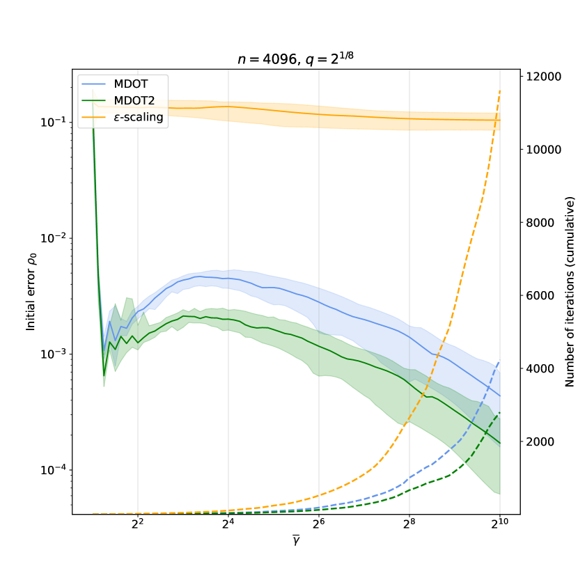
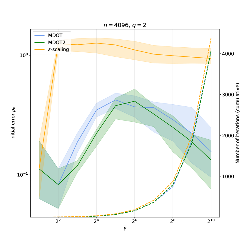
Figure 1: Comparison of $\varepsilon$-scaling warm-start to our formulas in (14-15), where we use the learning rate schedule $\overline{\gamma}_{t}=q\overline{\gamma}_{t-1}$ (suggested by Schmitzer (2019)) for $q{=}2^{1/8}$ (left) and $q{=}2$ (right). Evaluation is over 20 pairs of marginals with $n{=}4096$ and entropy uniformly sampled from $[0.1\log_{2}n,0.9\log_{2}n]$. Sinkhorn’s Alg. is used for Bregman projections. LHS of the $y$-axis measures marginal infeasibility at initialization $\rho_{0}$ (solid lines), while the RHS counts running total number of Sinkhorn iterations (dashed lines). Shaded areas show $80\%$ confidence intervals around the median. With small enough step sizes $\gamma_{t}$ ($q{=}2^{1/8}$), the formula in (15) shown in green (MDOT2) improves over (14). MDOT warm-start is more robust to $q$ than $\varepsilon$-scaling warm-start.

3.1.1 Warm-starting Bregman Projections

A key question that arises from this view asks how ${{\bm{z}}\coloneqq({\bm{u}},{\bm{v}})}$ should be initialized to solve problem (2.1) at each MD step given approximate $\overline{{\bm{z}}}\coloneqq(\overline{{\bm{u}}},\overline{{\bm{v}}})$ and ${\bm{z}}^{*}{\coloneqq}({\bm{u}}^{*},{\bm{v}}^{*})$ at prior $\overline{\gamma}_{t}$ and $\gamma_{t}$ respectively. The $\varepsilon$-scaling approach maintains reparamatrized dual variables ${\tilde{{\bm{z}}}\coloneqq\overline{{\bm{z}}}/\overline{\gamma}_{t}}$ as the temperature decays. Thus, $\tilde{{\bm{z}}}$ not being altered in any specific way following a temperature decrease amounts to predicting ${\overline{{\bm{z}}}(\overline{\gamma}_{t+1})\approx(\overline{\gamma}_{t+1}/\overline{\gamma}_{t})\overline{{\bm{z}}}(\overline{\gamma}_{t})}$, i.e., using an overly simplistic linear model in our parametrization. Here, we seek better ways to model the trajectory $\overline{{\bm{z}}}(\overline{\gamma})$.

A straightforward approach is to consider a Taylor expansion around recently visited $\overline{\gamma}$:

$$\overline{{\bm{z}}}(\overline{\gamma}_{t+1})\coloneqq\overline{{\bm{z}}}(\overline{\gamma}_{t})+\frac{\partial{\overline{{\bm{z}}}}}{\partial\overline{\gamma}}(\overline{\gamma}_{t})(\overline{\gamma}_{t+1}-\overline{\gamma}_{t})+\ldots$$ (12)

We consider a 1st order expansion. To approximate ${\partial{\overline{{\bm{z}}}}}/{\partial\overline{\gamma}}$ at $\overline{\gamma}_{t}$, we can use backward finite differencing:

$$\frac{\partial{\overline{{\bm{z}}}}}{\partial\overline{\gamma}}(\overline{\gamma}_{t})\approx\frac{\overline{{\bm{z}}}(\overline{\gamma}_{t})-\overline{{\bm{z}}}(\overline{\gamma}_{t-1})}{\overline{\gamma}_{t}-\overline{\gamma}_{t-1}}=\frac{{\bm{z}}^{*}(\gamma_{t-1})}{\gamma_{t-1}}.$$ (13)

Keeping the first two terms in (12) and rearranging:

$${\bm{z}}^{*}(\gamma_{t})\approx\frac{\gamma_{t}}{\gamma_{t-1}}{\bm{z}}^{*}(\gamma_{t-1}).$$ (14)

Intuitively, this captures the idea that we should scale the update vectors ${\bm{z}}^{*}$ by the ratio of consecutive dual space gradient step sizes $\gamma_{t}/\gamma_{t-1}$, instead of scaling the running sum of dual variables $\overline{{\bm{z}}}$ by the ratio of consecutive (inverse) temperatures $\overline{\gamma}_{t}/\overline{\gamma}_{t-1}$.

We also derive a more advanced backward finite difference formula than (14) that cancels 2nd order error terms in the approximation of $\partial{\overline{{\bm{z}}}}(\overline{\gamma}_{t})/\partial\overline{\gamma}$. The resulting warm-start guess is of the form:

$${\bm{z}}^{*}(\gamma_{t})\approx a{\bm{z}}^{*}(\gamma_{t-1})+b{\bm{z}}^{*}(\gamma_{t-2}),$$ (15)

where $a$ and $b$ are functions of $\gamma_{t},\gamma_{t-1},\gamma_{t-2}$ (see Appx. B.1 for the derivations and exact values).

3.1.2 Bregman Projection Stopping Criteria

Another issue related to warm-starting is how precise the Bregman projection (as measured by some convergence criterion $\rho$) at a given $\overline{\gamma}$ should be. For the final OT cost computed, errors incurred by an inexact projection onto ${\mathcal{U}}({\bm{r}},{\bm{c}})$ should be comparable in magnitude to errors incurred due to entropic regularization as in (10). Suppose that for some $\overline{\gamma}_{\mathrm{target}}$, $\rho$ being less than some threshold $\epsilon$ satisfies this requirement. Should the same $\epsilon$ be used for all projection problems throughout MD (e.g., as in Schmitzer (2019))?

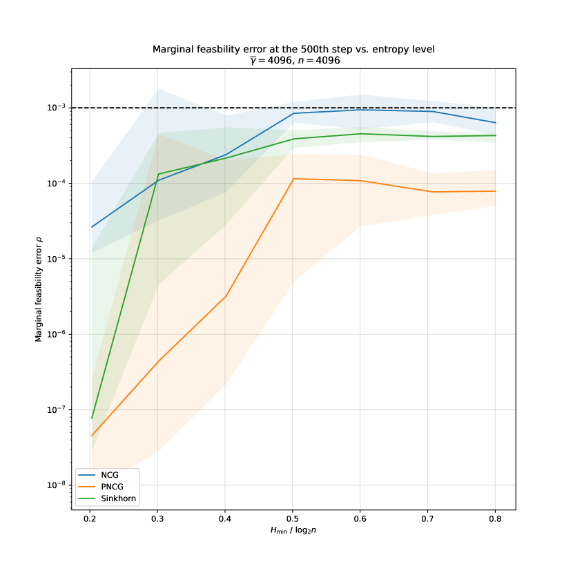
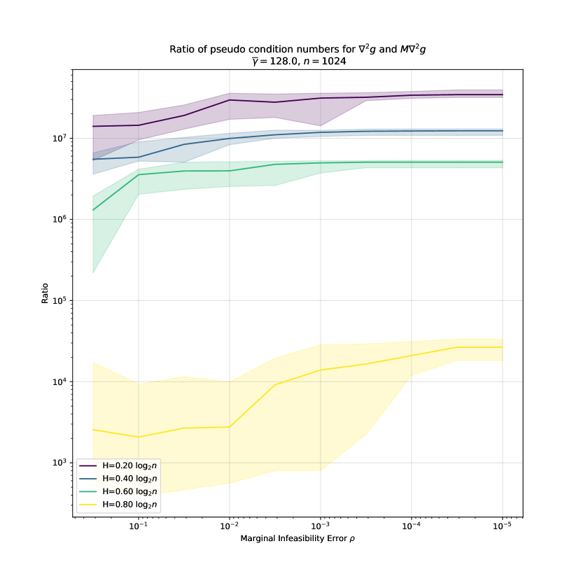
Figure 2: (Left) Marginal infeasibility $\rho$ after 500 iterations vs. entropy of marginals given ${n=4096}$, ${\overline{\gamma}=4096}$ and initial error $\rho_{0}\approx 10^{-3}$ (horizontal dashed line) for Sinkhorn (green), PNCG (orange) and the vanilla NCG (blue) algorithms. (Right) The ratio of pseudo-condition numbers for $\nabla^{2}g$ and $M\nabla^{2}g$ tends to increase with lower projection error $\rho$. Preconditioning is increasingly more effective for lower entropy marginals. This behavior is correlated with the growing performance difference between NCG vs. PNCG with decreasing entropy as seen on the left. Shaded areas show 60% confidence interval around the median over 30 runs.

The MD viewpoint suggests otherwise; intermediate projections serve only to improve the warm-starting for the next problem, and ultimately for the final problem. As warm-starting already admits approximation errors, over-optimizing to find near-exact values for ${\bm{z}}^{*}(\gamma)$ yields diminishing returns at high temperatures. Motivated by this argument and Prop. 3.2, we choose:

$$\epsilon(\overline{\gamma})=\tau H_{\min}/\overline{\gamma},$$ (16)

where $\tau\in(0,1)$ and the algorithm terminates when $\rho\coloneqq\left\lVert{\bm{r}}-{\bm{r}}(P)\right\rVert_{1}+\left\lVert{\bm{c}}-{\bm{c}}(P)\right\rVert_{1}\leq\epsilon$. Thanks to Lemma 7 of Altschuler et al. (2017), this choice guarantees that projection errors will not dominate errors stemming from high temperature at any given MD step (for small enough $\tau$). In Alg. 1, we write the resulting Mirror Descent Optimal Transport (MDOT) algorithm. While we omit specifying the particular Bregman projection algorithm used in L4 for generality, in the next section we introduce a new projection algorithm as an alternative to SA. The advantage of our warm-starting over the naive $\varepsilon$-scaling warm-starting can be seen in Fig. 1 (more detailed discussion in Sec. 4). Although we wrote MDOT in Alg. 1 using (14), Fig. 1 also investigates the use of (15) for $t>1$.

3.2 Preconditioned Non-linear Conjugate Gradients for
Bregman Projections

It is well-known that the convergence rate of SA declines at low temperatures (Kosowsky & Yuille, 1994). In search of a faster alternative suitable for MD, we turn to NCG methods. First, we consider the Hessian of the dual objective $g$ in (2.1) at $({\bm{u}},{\bm{v}})$:

$$\nabla^{2}g=\begin{pmatrix}\mathbf{D}({\bm{r}}(P))&P\\ P^{\top}&\mathbf{D}({\bm{c}}(P))\end{pmatrix},$$ (17)

which is degenerate with rank at most ${2n-1}$ owing to an eigenvector ${(\bm{1}_{n},-\bm{1}_{n})}$ with a zero eigenvalue. This is due to the well-known property that scalar shifts $({{\bm{u}}+\delta\bm{1}_{n}},{{\bm{v}}-\delta\bm{1}_{n}})$ yield the same $P({\bm{u}},{\bm{v}})$ and $g({\bm{u}},{\bm{v}})$ for any $\delta\in\mathbb{R}$, i.e., the objective is constant along this direction. Hence, when studying the scaling of the Hessian empirically, instead of the condition number $\lambda_{2n}/\lambda_{1}$, we heuristically consider a pseudo-condition number $\lambda_{2n}/\lambda_{2}$ given eigenvalues $0=\lambda_{1}\leq\cdots\leq\lambda_{2n}$.

A straightforward application of NCG to problem (2.1) requires only computing the gradient at $({\bm{u}},{\bm{v}})$:

$$\nabla g=\big{(}{\bm{r}}(P){-}{\bm{r}},~{}~{}{\bm{c}}(P){-}{\bm{c}}\big{)}.$$ (18)

To scale the Hessian, we instead consider replacing the gradient with the Sinkhorn direction:

$${\bm{s}}=\left(\log{\bm{r}}(P)-\log{\bm{r}},~{}~{}\log{\bm{c}}(P)-\log{\bm{c}}\right),$$ (19)

where $-{\bm{s}}$ is a descent direction for any $({\bm{u}},{\bm{v}})$:

$$\begin{split}\big{\langle}{\bm{s}},\nabla g\big{\rangle}&=D_{h}\big{(}{\bm{r}}(P)|{\bm{r}}\big{)}+D_{h}\big{(}{\bm{r}}|{\bm{r}}(P)\big{)}\\ &+D_{h}\big{(}{\bm{c}}(P)|{\bm{c}}\big{)}+D_{h}\big{(}{\bm{c}}|{\bm{c}}(P)\big{)}\geq 0.\end{split}$$

Algorithm 2 PNCGProject$(\overline{\gamma}C,\overline{{\bm{z}}},{\bm{z}},{\bm{r}},{\bm{c}},\epsilon)$

1:$(\overline{{\bm{u}}}_{\mathrm{init}},\overline{{\bm{v}}}_{\mathrm{init}})\leftarrow\overline{{\bm{z}}},~{}~{}({\bm{u}},{\bm{v}})\leftarrow{\bm{z}}$

2:$\overline{{\bm{u}}}\leftarrow\overline{{\bm{u}}}_{\mathrm{init}}+{\bm{u}},~{}~{}\overline{{\bm{v}}}\leftarrow\overline{{\bm{v}}}_{\mathrm{init}}+{\bm{v}}$

3:$\log{\bm{r}}(P)\leftarrow\overline{{\bm{u}}}+\mathrm{LogSumExp}_{j}(\bm{1}_{n}\overline{{\bm{v}}}^{\top}-\overline{\gamma}C)$

4:$\log{\bm{c}}(P)\leftarrow\overline{{\bm{v}}}+\mathrm{LogSumExp}_{i}(\overline{{\bm{u}}}\bm{1}_{n}^{\top}-\overline{\gamma}C)$

5:$\rho\leftarrow\left\lVert{\bm{r}}-{\bm{r}}(P)\right\rVert_{1}+\left\lVert{\bm{c}}-{\bm{c}}(P)\right\rVert_{1}$

6:while $\rho>\epsilon$ do

7:     Evaluate $\nabla g$ and ${\bm{s}}$ at $(\overline{{\bm{u}}},\overline{{\bm{v}}})$ $\triangleright$ (18-19)

8:     ${\bm{p}}\leftarrow-{\bm{s}}+\beta{\bm{p}}$ $\triangleright$ (20)

9:     if $\langle{\bm{p}},\nabla g\rangle<0$ then

10:         ${\bm{p}}\leftarrow-{\bm{s}}$ $\triangleright$ Reset CG

11:     end if

12:     $\alpha,\log{\bm{r}}(P),\log{\bm{c}}(P)\leftarrow\textrm{LineSearch}({\bm{p}},\overline{{\bm{u}}},\overline{{\bm{v}}})$

13:     $\overline{{\bm{u}}}\leftarrow\overline{{\bm{u}}}+\alpha{\bm{p}}_{\bm{u}},\overline{{\bm{v}}}\leftarrow\overline{{\bm{v}}}+\alpha{\bm{p}}_{\bm{v}}$

14:     $\rho\leftarrow\left\lVert{\bm{r}}-{\bm{r}}(P)\right\rVert_{1}+\left\lVert{\bm{c}}-{\bm{c}}(P)\right\rVert_{1}$

15:end while

16:Output ${\bm{z}}\leftarrow(\overline{{\bm{u}}}-\overline{{\bm{u}}}_{\mathrm{init}},\overline{{\bm{v}}}-\overline{{\bm{v}}}_{\mathrm{init}})$

One interpretation of this choice of descent direction is as a preconditioning of the system. In particular, observe that ${\bm{s}}({\bm{u}},{\bm{v}})=M\nabla g({\bm{u}},{\bm{v}})$, where the diagonal preconditioner ${M=\mathbf{D}\left({\bm{s}}({\bm{u}},{\bm{v}})/\nabla g({\bm{u}},{\bm{v}})\right)}$. In Sec. 4, we empirically show that the pseudo-condition number of $M\nabla^{2}g$ is markedly lower than that of $\nabla^{2}g$ across a variety of problems and the preconditioned NCG (PNCG) approach behaves much better particularly over lower entropy marginals. This observation is a key finding of this work as it facilitates significant performance gains over a naive application of NCG.

Given ${\bm{s}}^{k}$ and $\nabla g^{k}$ at each step $k$, we compute $\beta_{k}$ via the formula for preconditioned Polak-Ribiere (PPR) by Al-Baali & Fletcher (1996) (cf. (6)) :

$$\beta_{k}^{PPR}=\frac{\langle\nabla g^{k}-\nabla g^{k-1},{\bm{s}}^{k}\rangle}{\langle\nabla g^{k-1},{\bm{p}}^{k-1}\rangle},$$ (20)

where $\beta_{1}^{PPR}=0$ (see Alg. 2). While we defer details of the line search in L12 of Alg. 2 to Appx. C, we note that by design, our line search carries out cost $O(n^{2})$ LogSumExp operations necessary to compute the Sinkhorn direction at the next iteration; as a result, an average iteration of PNCG in high dimensions costs ${\approx 1.5{-}2.5\times}$ a row+column update in SA.

4 EXPERIMENTS

In this section, we first empirically investigate the questions below on a synthetic dataset and compare the behavior of proposed algorithms:

1. Does our warm-starting provide performance gains over the implicit warm-starting in $\varepsilon$-scaling?

2. Does employing Sinkhorn directions (preconditioning) instead of the vanilla NCG improve the local convergence of NCG? If so, under what conditions with respect to the entropy of ${\bm{r}},{\bm{c}}$?

3. How does the PNCG approach compare to Sinkhorn iteration in terms of projection speed, problem size $n$ and entropy of ${\bm{r}},{\bm{c}}$?

In Sec. 4, we compare the proposed algorithms to log-domain stabilized SA, Mirror Sinkhorn (MSK) by Ballu & Berthet (2022), and Alg. 3.5 of Feydy (2020) over upsampled MNIST images. All experiments are performed on an NVIDIA GeForce RTX 2080 Ti GPU with 64-bit precision. Unless otherwise stated, all transport plans are rounded onto ${\mathcal{U}}({\bm{r}},{\bm{c}})$ via Alg. 2 of Altschuler et al. (2017) after processing; time taken by the rounding algorithm is not included in wall-clock time measurements. In all experiments, $\tau=10^{-3}$.

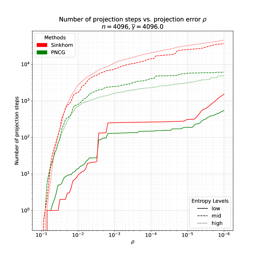
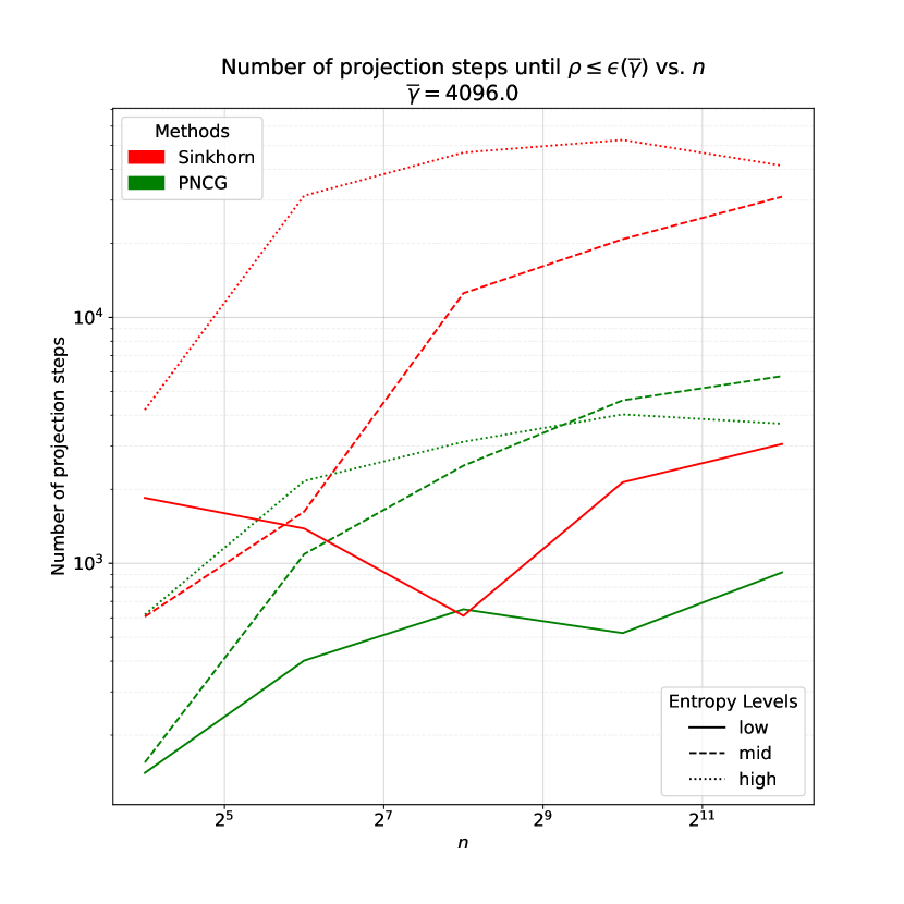
Figure 3: (Left) Number of iterations vs. marginal infeasibility $\rho$ for Sinkhorn and PNCG projections given ${n=4096}$, $\overline{\gamma}=4096$, $\rho_{0}\approx 10^{-1}$ over $H({\bm{r}})$ and $H({\bm{c}})$ both approx. $\{0.1\log_{2}n,0.5\log_{2},0.9\log_{2}n\}$. (Right) Number of iterations until $\rho\leq\epsilon(\overline{\gamma})$ vs. problem size $n$. All lines display the median over 16 samples of ${\bm{r}},{\bm{c}},C$.

We remark that while we benchmark on problems with $n{=}4096$, this choice only reflects our aspiration to run a large number of tests per configuration and gather statistically significant results, but no inherent limitations of the algorithm. Our code supports the use of on-the-fly CUDA kernels to evaluate entries of the cost matrix on the go using the PyKeOps package (Charlier et al., 2021). In this case, MDOT has a memory footprint of $O(n)$ rather than $O(n^{2})$; it has been verified to scale to much larger problems ($n\approx 100,000$).

4.1 Ablations over Synthetic Datasets

For the experiments here, we randomly sample a cost matrix $C$ and marginals with entropy $H({\bm{r}})\approx H({\bm{c}})\in[0.1\log_{2}n,0.9\log_{2}n]$ (see Appx. D for details on the data generation process). This setup allows us to highlight the importance of marginal entropy (see (10)) in computational OT and study the convergence behavior of the algorithms in a controlled manner.

Q1. In Fig. 1, we compare the MDOT warm-starting (Sec. 3.1.1) to that of $\varepsilon$-scaling strategies. The experiments are carried out with ${n{=}4096}$ over marginals with entropy values sampled uniformly from $[0.1\log_{2}n,0.9\log_{2}n]$. To control for any effects due to the newly introduced PNCG algorithm, we use SA for Bregman projections. We see a clear advantage of the MDOT warm-starting with lower initial error $\rho_{0}$ relative to the $\varepsilon$-scaling formulation. Schmitzer (2019) suggested that too slow temperature decay schedules may increase numerical overhead; we show that this overhead can be overcome with more accurate warm-starting. Indeed, Fig 1 shows that MDOT is $3-4\times$ faster than $\varepsilon$-scaling under a slow decay schedule ($q{=}2^{1/8}$) and is marginally faster for a rapid decay schedule ($q{=}2$). Unlike $\varepsilon$-scaling warm-start, the total number of iterations required by MDOT is insensitive to $q$ in this range ($\approx 4000$ iterations).

Q2. In Fig. 2, we study Q2 by comparing vanilla NCG to PNCG, as well as SA. We sample marginals with entropies ranging between $[0.2\log_{2}n,0.8\log_{2}n]$. Then, we precompute ${(\overline{{\bm{u}}},\overline{{\bm{v}}})}$ such that ${\rho\approx 10^{-3}}$ and run each algorithm for 500 projection steps. The results suggest that NCG is especially slow for low-entropy marginals. As seen in (17), many rows/columns of $\nabla^{2}g$ may consist entirely of near-zero entries if the marginals ${\bm{r}},{\bm{c}}$ are low-entropy (and therefore contain many near-zero entries). This makes the approximate rank of the Hessian much smaller than $n$. Indeed, in Fig. 2 (right), we plot the ratio of the pseudo-condition number for $\nabla^{2}g$ and $M\nabla^{2}g$ over PNCG iterations at each entropy level) over a simpler problem (due to the high cost of eigendecomposition); preconditioning vastly reduces $\lambda_{2n}/\lambda_{2}$ and the extent of reduction gradually increases with lower entropy distributions. However, even in the high-entropy setting where preconditioning has a milder effect, PNCG still outperforms NCG (as well as SA). Thus the results suggest that preconditioning is essential for NCG algorithms to be broadly effective for OT.

Q3. In Fig. 3 (left), we compare PNCG to SA in terms of convergence speed given distributions with low, medium and high entropy, where each projection problem is initialized such that $\rho_{0}\approx 10^{-1}$ at $\overline{\gamma}{=}4096$. For both algorithms, problems with low entropy marginals are solved much more quickly than those with mid/high entropy. PNCG enjoys a better dependence on $\rho$ than SA (as the performance gap grows with decreasing $\rho$) across all entropy levels (except in case of low entropy, far from optima). Further, it handles high entropy better than SA. On the right side of Fig. 3, we repeat the same experiments, but this time continuing projections only until the stopping criterion discussed in Sec. 3.1.2 is satisfied, while varying $n\in[16,4096]$. We verify that the dependence of PNCG on $n$ is similar to SA, and does not suffer from any unexpected pathologies.

4.2 Benchmarking on Upsampled MNIST

In this section, we evaluate PNCG and MDOT on the MNIST dataset in line with prior work (Cuturi, 2013; Altschuler et al., 2017; Lin et al., 2022). We upsample images so that ${n{=}4096}$ (data generation details are deferred to Appx. D). For MDOT, we use the schedule $\overline{\gamma}_{t}{=}q\overline{\gamma}_{t-1}$, where $q{=}2$ and $\gamma_{0}{=}\min(\overline{\gamma}_{\mathrm{target}},2^{6})$. For the closely related Mirror Sinkhorn (MSK) algorithm of Ballu & Berthet (2022) the variable step size schedule prescribed by their Thm. 3.3 is used. For Alg. 3.5 of Feydy (2020), we evaluate both their fast and safe settings, which set $q{=}2$ and $q{=}0.9^{-1}$ respectively.

While MDOT optimizes dual variables to convergence between MD steps, Alg. 3.5 of Feydy (2020) performs a single (symmetrized) Sinkhorn update before a temperature decay, i.e., it does not decrease consecutive Bregman projection objectives sufficiently despite taking increasingly large gradient steps in the dual space (cf. 4). This causes an accumulation of projection errors and consequently performs poorly in terms of precision if the dual variables $\overline{{\bm{u}}},\overline{{\bm{v}}}$ found by the algorithm are used to compute a plan $P$ as in (1) before rounding onto ${\mathcal{U}}({\bm{r}},{\bm{c}})$. Their debiasing option for estimating the OT distance via Sinkhorn divergences (introduced by Ramdas et al. (2017)) fares slightly better and is used here to comprise a stronger baseline, albeit this approach does not find a member of ${\mathcal{U}}({\bm{r}},{\bm{c}})$, which may be a strict requirement in some applications.

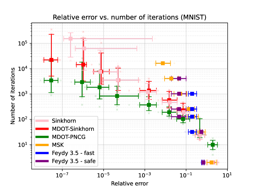
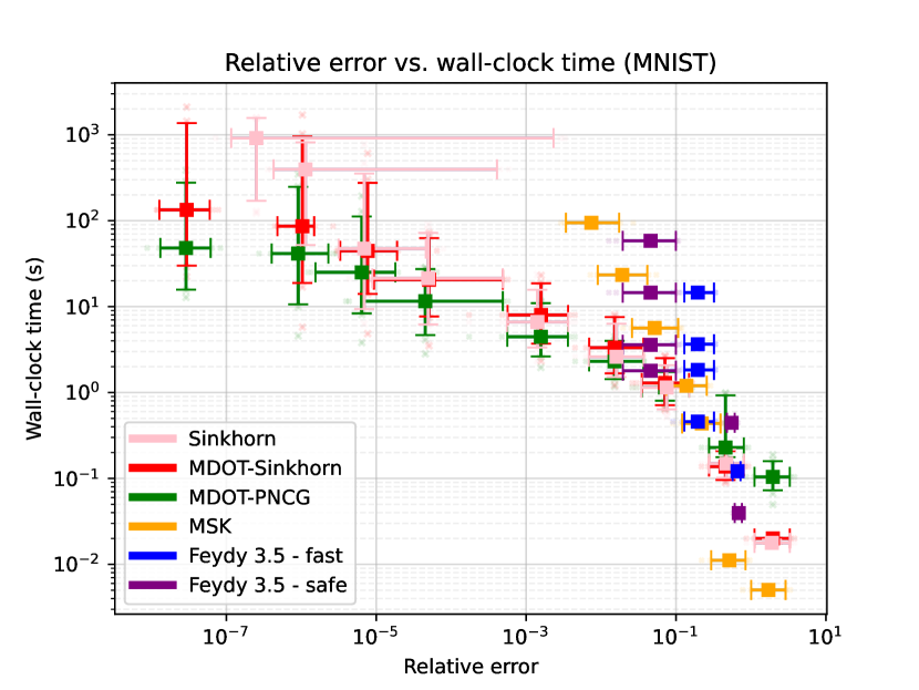
Figure 4: Total number of projection iterations (left) and wall-clock time (right) against relative error ${\langle P-P^{*},C\rangle/\langle P^{*},C\rangle}$ over the upsampled MNIST dataset. For MDOT, target values of $\overline{\gamma}$ span the range $[2^{2},2^{19}]$ with $\gamma_{0}=\min(\overline{\gamma},2^{6})$ in all experiments. For the MSK algorithm of Ballu & Berthet (2022) and Alg. 3.5 of Feydy (2020), we fix the total number of iterations at each displayed marker on the left. Error bars mark $90\%$ confidence intervals across 32 sample pairs $({\bm{r}},{\bm{c}})$ for respective axes. Solid squares mark the median values.

Fig. 4 shows that neither of the settings for Alg. 3.5 of Feydy (2020) is able to reach relative error below $1\%$. MSK also runs a single row/column scaling update after a dual space gradient step, but takes increasingly smaller steps and maintains a running average of transport plans to ensure convergence. It performs well down to 10% relative error, but decreasing step sizes gradually slow it down. Log-domain stabilized SA is competitive down to relative error $10^{-5}$, but its performance degrades rapidly past temperatures below $2^{-10}$; at relative error $10^{-6}$ it takes $10\times$ as much time as MDOT-PNCG and sometimes does not terminate in the maximum number of allowed steps (${\approx}200k$), resulting in high relative error due to dominating projection errors. Computing approximations beyond $10^{-7}$ precision with SA becomes impractical. MDOT-PNCG is the quickest to converge for relative error below $10^{-3}$. The performance gap with its close second, MDOT-Sinkhorn, grows with higher precision.

5 RELATED WORK

Acceleration of OT solvers has been a highlight of machine learning research since the seminal work of Cuturi (2013). For instance, Altschuler et al. (2017) proposed the Greenkhorn algorithm, which greedily selects individual rows or columns to scale at a given step and requires fewer row/column updates than SA to converge, but practical speedup over GPUs has not been demonstrated to the best of our knowledge. Dvurechensky et al. (2018) proposed an adaptive primal-dual accelerated gradient descent (APDAGD) algorithm. Lin et al. (2019) later proposed adaptive primal-dual accelerated mirror descent (APDAMD) with theoretical guarantees. Empirically, APDAMD was shown to outperform APDAGD in terms of number of iterations, but not SA. However, these tests only covered a high relative error regime (${{>}50\%}$). Modest gains over SA in terms of number of iterations in the same regime were later obtained by Lin et al. (2022) via an accelerated alternating minimization (AAM) algorithm similar to that of Guminov et al. (2021). Notably, APDAMD applies MD to the entropic problem (2.1), while we apply it to problem (2.1).

Application of MD to (2.1) has also been considered. Yang & Toh (2022) discuss an algorithm similar to MDOT, although their approach differs from ours in a number of important aspects. Most notably, they require a rounding procedure onto ${\mathcal{U}}({\bm{r}},{\bm{c}})$ after each MD step, as well as the verification of complicated stopping criteria for all Bregman projections, while we did not find these to be necessary experimentally or mathematically. As discussed in detail in Sec. 3.1, well-known $\varepsilon$-scaling strategies are also closely related (Kosowsky & Yuille, 1994; Schmitzer, 2019).

Recently, Ballu & Berthet (2022) introduced MSK, which takes gradient steps in the dual space as in (4), but instead of subsequently projecting onto ${\mathcal{U}}({\bm{r}},{\bm{c}})$, projects onto ${\mathcal{U}}(\cdot,{\bm{c}})$ or ${\mathcal{U}}(\cdot,{\bm{r}})$ via a single row/column update. Our experiments suggested that this approach is only efficient in the high relative error regime (see Fig. 4). Further, MSK requires maintaining a running average of transport plans $P$, which brings to question the possibility of an implementation with $O(n)$ memory footprint. Xie et al. (2020) previously proposed an algorithm (IPOT) similar to MSK with a fixed, even number of Sinkhorn updates (usually 2) following gradient steps; we omitted additional empirical comparison to IPOT given its similarity with MSK. Alg. 3.5 of Feydy (2020) is also similar to these algorithms in spirit and was thoroughly discussed in Sec. 4.

An orthogonal direction of practical accelaration research involves multi-scale strategies, which use clustering or grids to solve a sequence of coarse-to-fine OT problems and are sometimes combined with $\varepsilon$-scaling (Schmitzer, 2016, 2019; Feydy, 2020). These are known to provide performance gains when the marginals are defined over well-clustered particles or in low-dimensional event spaces (Peyré et al., 2019). Lastly, in a similar spirit to PNCG, curvature-aware convex optimization techniques such as L-BFGS have also been considered for OT, e.g., Mérigot (2011); Blondel et al. (2018); however, scalability, precision and better performance than SA on GPUs has not been demonstrated simultaneously to our knowledge.

6 CONCLUSION

In this work, we first presented a general MD procedure for computing OT distances with high accuracy and described its relation to well-known $\varepsilon$-scaling strategies. The algorithm employs a warm-starting of dual variables for Bregman projection problems in MD, which was empirically shown to be highly effective. To address the declining convergence rate of Sinkhorn iteration as MD proceeds, we then presented a new conjugate gradients algorithm, PNCG, for Bregman projections onto the transportation polytope. The algorithm was shown to outperform Sinkhorn iteration and other recent baselines in terms of wall-clock time, especially in the high precision regime, and is especially well-suited for OT problems involving high-entropy marginals. Future work may explore the convergence behavior of PNCG theoretically or combine MDOT with multi-scale strategies.

A Background (Extended Version)

A.1 Optimal Transport

Given a cost matrix ${C\in{[0,1]}^{n\times n}}$, where $C_{ij}$ is the cost of transportation between ${{\bm{x}}_{i},{\bm{x}}_{j}\in{\mathcal{X}}}$, and marginal distributions ${{\bm{r}},{\bm{c}}\in\Delta_{n}}$, we study the optimal transport problem given by the following: [2] P ∈U(r, c)⟨P, C ⟩. Since the problem is a linear program (LP), the optimal transport plan need not be unique. Entropic regularization of the problem is often used for more efficient computation on GPUs (Cuturi, 2013): [2] P ∈U(r, c)⟨P, C ⟩- 1γH(P) where $\gamma>0$ and $H(P)=-\sum_{ij}P_{ij}\log P_{ij}$ is the Shannon entropy of the joint distribution $P$, hence the term entropic regularization. The formulation is derived by adding an additional KL divergence constraint to (2.1) requiring $D_{\mathrm{KL}}(P|{\bm{r}}{\bm{c}}^{\top})\leq\zeta$, where ${\bm{r}}{\bm{c}}^{\top}$ is the independent coupling of $({\bm{r}},{\bm{c}})$, ${\zeta>0}$, and ${D_{\mathrm{KL}}(P|{\bm{r}}{\bm{c}}^{\top})=\sum_{ij}P_{ij}\log\left(\frac{P_{ij}}{r_{i}c_{j}}\right)}$ with the convention that $0/0=1$. The Lagrangian for the primal problem in (2.1) is given by the following,

$${\mathcal{L}}(P,\mathbf{\bm{\alpha}},\bm{\beta},\gamma)=\langle P,C\rangle+\langle\mathbf{\bm{\alpha}},{\bm{r}}-P\bm{1}_{n}\rangle+\langle\bm{\beta},{\bm{c}}-P^{T}\bm{1}_{n}\rangle-\frac{1}{\gamma}H(P),$$ (21)

where $\bm{\alpha},\bm{\beta}\in\mathbb{R}^{n}$ are dual variables and a smaller $\gamma$ corresponds to a larger $\zeta$. The negative entropy term renders the Lagrangian strictly convex in $P$, for which a unique solution with respect to $P$ can be shown to exist with ease:

$$\frac{\partial{\mathcal{L}}}{\partial P_{ij}}=C_{ij}-\alpha_{i}-\beta_{j}+\frac{1}{\gamma}(1+\log P_{ij})=0\iff P_{ij}=e^{\gamma\alpha_{i}-1/2}e^{-\gamma C_{ij}}e^{\gamma\beta_{j}-1/2}.$$ (22)

With a reparametrization choosing $u_{i}=\gamma\alpha_{i}-1/2$ and $v_{j}=\gamma\beta_{j}-1/2$, plugging $P_{ij}$ given by (1) into the Lagrangian results in the following unconstrained dual problem: [2] u, v∈R^n∑_ij exp { u_i + v_j - γC_ij } - ⟨u, r⟩- ⟨v, c⟩

Algorithm 3 SinkhornProject$(\overline{\gamma}C,\overline{{\bm{z}}},{\bm{z}},{\bm{r}},{\bm{c}},\epsilon)$

1:$(\overline{{\bm{u}}}_{\mathrm{init}},\overline{{\bm{v}}}_{\mathrm{init}})\leftarrow\overline{{\bm{z}}},~{}~{}({\bm{u}},{\bm{v}})\leftarrow{\bm{z}}$

2:$\overline{{\bm{u}}}\leftarrow\overline{{\bm{u}}}_{\mathrm{init}}+{\bm{u}},~{}~{}\overline{{\bm{v}}}\leftarrow\overline{{\bm{v}}}_{\mathrm{init}}+{\bm{v}}$

3:$\log{\bm{r}}(P)\leftarrow\overline{{\bm{u}}}+\mathrm{LogSumExp}_{j}(\bm{1}_{n}\overline{{\bm{v}}}^{\top}-\overline{\gamma}C)$

4:$\log{\bm{c}}(P)\leftarrow\overline{{\bm{v}}}+\mathrm{LogSumExp}_{i}(\overline{{\bm{u}}}\bm{1}_{n}^{\top}-\overline{\gamma}C)$

5:$\rho\leftarrow\left\lVert{\bm{r}}-{\bm{r}}(P)\right\rVert_{1}+\left\lVert{\bm{c}}-{\bm{c}}(P)\right\rVert_{1}$ $\triangleright$ $\rho({\bm{u}},{\bm{v}})=\left\lVert\nabla g({\bm{u}},{\bm{v}})\right\rVert_{1}$

6:while $\rho>\epsilon$ do

7:     $\overline{{\bm{u}}}\leftarrow\overline{{\bm{u}}}+\log{\bm{r}}-\log{\bm{r}}(P)$

8:     $\log{\bm{c}}(P)\leftarrow\overline{{\bm{v}}}+\mathrm{LogSumExp}_{i}(\overline{{\bm{u}}}\bm{1}_{n}^{\top}-\overline{\gamma}C)$

9:     $\overline{{\bm{v}}}\leftarrow\overline{{\bm{v}}}+\log{\bm{c}}-\log{\bm{c}}(P)$

10:     $\log{\bm{r}}(P)\leftarrow\overline{{\bm{u}}}+\mathrm{LogSumExp}_{j}(\bm{1}_{n}\overline{{\bm{v}}}^{\top}-\overline{\gamma}C)$

11:     $\rho\leftarrow\left\lVert{\bm{r}}-{\bm{r}}(P)\right\rVert_{1}$

12:end while

13:$\overline{{\bm{u}}}\leftarrow\overline{{\bm{u}}}+\log{\bm{r}}-\log{\bm{r}}(P)$

14:Output ${\bm{z}}\leftarrow(\overline{{\bm{u}}}-\overline{{\bm{u}}}_{\mathrm{init}},\overline{{\bm{v}}}-\overline{{\bm{v}}}_{\mathrm{init}})$

The SA algorithm (see Alg. 3) can be used to optimize this objective and approximately project $\exp{\{-\gamma C_{ij}\}}$ onto ${\mathcal{U}}({\bm{r}},{\bm{c}})$ given some stopping criterion measured by a distance or divergence $d$. The updates are guaranteed to converge to dual-optimal values as the number of iterations $k\rightarrow\infty$ (Sinkhorn & Knopp, 1967; Sinkhorn, 1967; Franklin & Lorenz, 1989; Knight, 2008). Later, the procedure and its variants were shown to converge in $\widetilde{O}(n^{2})$ iterations with other terms depending on the level of desired accuracy (Altschuler et al., 2017). The optimal solution of (2.1) converges to the solution of (2.1) as $\gamma\rightarrow\infty$ (Cuturi, 2013).

A.2 Mirror Descent

To solve problem (2.1), we rely on mirror descent. Hence, we introduce the necessary background in this section. Originally proposed by Nemirovski & Yudin (1983), mirror descent can be viewed as a generalization of gradient descent. To establish the connection, we first need to define Bregman divergences. Let ${\mathcal{D}}\subset\mathbb{R}^{n}$ be a convex, open set. The Bregman divergence between a pair of points ${\bm{x}},{\bm{y}}\in{\mathcal{D}}$ under a strictly convex and differentiable function $h:{\mathcal{D}}\rightarrow\mathbb{R}$ is given by

$$D_{h}({\bm{y}}|{\bm{x}})=h({\bm{y}})-h({\bm{x}})-\langle\nabla h({\bm{x}}),{\bm{y}}-{\bm{x}}\rangle.$$ (3 revisited)

That is, the Bregman divergence $D_{h}({\bm{y}}|{\bm{x}})$ is the difference between $h({\bm{y}})$ and its first-order approximation around ${\bm{x}}$. Since $h$ is convex by construction, the divergence value is always non-negative (by the first-order condition for convexity). Then, given a non-empty convex set ${\mathcal{F}}$ of feasible points such that ${\mathcal{F}}$ is included in the closure of ${\mathcal{D}}$ and ${\mathcal{F}}\cap{\mathcal{D}}\neq\emptyset$, an objective function $f:\mathbb{R}^{n}\rightarrow\mathbb{R}$ and an initial ${\bm{x}}^{0}\in{\mathcal{D}}$, mirror descent algorithms perform the following updates:

$${\bm{x}}^{t+1}=\operatorname*{arg\,min}_{{\bm{x}}\in{\mathcal{F}}\cap{\mathcal{D}}}\{\langle\nabla f({\bm{x}}^{t}),{\bm{x}}\rangle+\frac{1}{\gamma_{t}}D_{h}({\bm{x}}|{\bm{x}}^{t})\},$$ (2 revisited)

where $\gamma_{t}^{-1}>0$ is a (possibly time-varying) regularization weight. Equivalently:

$$\hat{{\bm{x}}}^{t+1}=\nabla h^{-1}\left(\nabla h({\bm{x}}^{t})-\gamma_{t}\nabla f({\bm{x}}^{t})\right)$$ (4 revisited)

$${\bm{x}}^{t+1}=\operatorname*{arg\,min}_{{\bm{x}}\in{\mathcal{F}}\cap{\mathcal{D}}}D_{h}({\bm{x}}|\hat{{\bm{x}}}^{t+1}),$$ (5 revisited)

where $h$ is strictly convex and $\nabla h:{\mathcal{D}}\rightarrow\mathbb{R}^{n}$ is called the mirror map as it maps ${\bm{x}}$ from the primal to the dual space. Here, (4) takes a gradient step in the dual space and maps the new point back onto the primal space, while (5) defines a Bregman projection of $\hat{{\bm{x}}}^{t+1}$ onto the feasible set ${\mathcal{F}}$ in the primal space. For further technical definitions and requirements on $h$ to ensure the existence and uniqueness of Bregman projections, see §4.1 of Bubeck (2015).

In the unconstrained case (i.e., ${{\mathcal{F}}={\mathcal{D}}}$) with ${{h({\bm{x}})=\frac{1}{2}\left\lVert{\bm{x}}\right\rVert_{2}^{2}}}$ (which yields ${{D_{h}({\bm{y}}|{\bm{x}})=\frac{1}{2}\left\lVert{\bm{y}}-{\bm{x}}\right\rVert_{2}^{2}}}$ and ${\nabla h({\bm{x}})={\bm{x}}}$), one recovers the standard gradient descent algorithm with step sizes $\gamma_{t}$. Otherwise, a Bregman projection onto ${\mathcal{F}}$ as in (5) is necessary if the minimizer in ${\mathcal{D}}$ lies outside ${\mathcal{F}}$, in which case one recovers the projected gradient descent method (once again) for ${h({\bm{x}})=\frac{1}{2}\left\lVert{\bm{x}}\right\rVert_{2}^{2}}$. Another common choice for $h$ is the negative entropy ${h({\bm{x}})=\sum_{i=1}^{n}x_{i}\log(x_{i})}$, which yields ${D_{h}({\bm{y}}|{\bm{x}})=D_{\mathrm{KL}}({\bm{y}}|{\bm{x}})}$ on the simplex $\Delta_{n}$. In general, for ${\bm{x}},{\bm{y}}\in\mathbb{R}^{n}_{>0}$ we have ${D_{h}({\bm{y}}|{\bm{x}})=\sum_{i}x_{i}-y_{i}+y_{i}\log(y_{i}/x_{i})}$. Since the OT objective in (2.1) is linear, we state the following result of interest.

Lemma A.1 (A mirror descent bound for linear objectives).

Given a linear objective function ${f({\bm{x}})=\langle{\bm{x}},{\bm{w}}\rangle}$, an initial point ${\bm{x}}^{0}\in{\mathcal{F}}$, an optimal point ${\bm{x}}^{*}$ and any $T>0$, a sequence $[{\bm{x}}^{t}]_{t\in\mathbb{N}}$ obtained via (2) satisfies:

$$f({\bm{x}}^{T})-f({\bm{x}}^{*})\leq\frac{D_{h}({\bm{x}}^{*}|{\bm{x}}^{0})}{\sum_{t=0}^{T-1}{\gamma_{t}}}.$$ (23)

For the proof, see Appx. B.

A.3 Conjugate Gradients

Initially proposed to solve linear systems of equations, or equivalently, unconstrained quadratic minimization problems, conjugate gradient (CG) methods aim to bridge steepest descent methods and Newton’s method in terms of convergence properties while retaining low memory and computational requirements (Fox et al., 1948; Forsythe et al., 1951; Hestenes & Stiefel, 1952). Later, they were extended for minimization of general non-linear objectives by Fletcher & Reeves (1964). In the context of quadratic minimization, one ensures the conjugacy property between all descent directions ${\bm{p}}^{k}\in\mathbb{R}^{n}$ up to and including the $k^{th}$ step, namely by requiring that they satisfy $({\bm{p}}^{k})^{\top}H{\bm{p}}^{k^{\prime}}=0$ for any $k,k^{\prime}\in[1\cdots k]$ and $k\neq k^{\prime}$, where $H\in\mathbb{R}^{n\times n}$ is the Hessian of the quadratic $f:\mathbb{R}^{n}\rightarrow\mathbb{R}$. It is well-known that when such descent directions are generated, the iterates ${\bm{x}}^{k+1}\leftarrow{\bm{x}}^{k}+\alpha{\bm{p}}^{k}$ with the step size $\alpha\in\mathbb{R}$ chosen to be the minimizer of the 1D quadratic along ${\bm{p}}^{k}$ will converge to the optimum in at most $n$ steps (Nocedal & Wright, 2006). Furthermore, if the number $m$ of distinct eigenvalues of $H$ is less than $n$, the method converges in $m$ iterations instead, while in general the objective decreases more quickly when eigenvalues form a small number of tight clusters (Stiefel, 1958; Kaniel, 1966; Nocedal & Wright, 2006).

A key appealing property of CG methods stems from the ability to generate descent directions satisfying the conjugacy property by considering only the last descent direction rather than all past descent directions. In particular, by taking ${\bm{p}}^{0}=-\nabla f({\bm{x}}^{0})$ and ${\bm{p}}^{k+1}\leftarrow-\nabla f({\bm{x}}^{k})+\beta_{k}{\bm{p}}^{k}$ where $\beta_{k}=\left\lVert\nabla f({\bm{x}}^{k})\right\rVert^{2}/\left\lVert\nabla f({\bm{x}}^{k-1})\right\rVert^{2}$, one can ensure conjugacy for quadratics given exact line search, i.e., optimal $\alpha$. Hence, the algorithm does not require storing a long history of past descent directions or Hessian approximations. We refer the reader to Algorithm 5.2 of Nocedal & Wright (2006) for further details. Fletcher & Reeves (1964) made the important observation that virtually the same algorithm can be used to minimize general non-linear objectives and without requiring exact line search. It was shown by Zoutendijk (1970) that the Fletcher-Reeves (FR) method converges with exact line search. Later, Al-Baali (1985) provided convergence results under certain assumptions on the objective function and an inexact line search. However, the FR method is known to produce unproductive descent directions with a small angle between them in some cases, thereby slowing down convergence (Gilbert & Nocedal, 1992). This motivated a slew of different approaches to compute $\beta_{k}$ (Nocedal & Wright, 2006). Of particular relevance to our efforts is the Polak-Ribiere (PR) method, which ameloriates the issue (Nocedal & Wright, 2006):

$$\beta_{k}^{PR}=\frac{\langle\nabla f({\bm{x}}^{k})-\nabla f({\bm{x}}^{k-1}),\nabla f({\bm{x}}^{k})\rangle}{\left\lVert\nabla f({\bm{x}}^{k-1})\right\rVert^{2}}.$$ (6 revisited)

As noted by Nocedal & Wright (2006), “nonlinear conjugate gradient methods possess surprising, sometimes bizarre, convergence properties”. Proofs of convergence are typically easier to obtain than are rates of convergence (see Ch. 3 of Andrei (2020) for such results). However, one practical way to improve the convergence rate of linear and non-linear CG (NCG) is via preconditioning. By making a change of variables ${\bm{x}}=S\hat{{\bm{x}}}$, one reduces the condition number of the problem and/or renders the eigenvalues of the reparametrized problem more tightly clustered relative to the original for improved convergence (ideally, $SS^{\top}\approx\nabla^{2}f^{-1}$). For further details on CG methods, we refer the reader to the survey by Hager & Zhang (2006b).

A.4 Line Search

Given a descent direction ${\bm{p}}^{k}\in\mathbb{R}^{n}$, i.e., a direction that satisfies $\langle{\bm{p}}^{k},\nabla f({\bm{x}}^{k})\rangle\leq 0$, line search algorithms aim to find an appropriate step size $\alpha$, where ${\bm{x}}^{k+1}\leftarrow{\bm{x}}^{k}+\alpha{\bm{p}}^{k}$. Perhaps the most well-known of desirable properties that a step size $\alpha$ should satisfy at any given optimization step are the Wolfe conditions (Wolfe, 1969, 1971). Given $\phi(\alpha)\coloneqq f({\bm{x}}^{k}+\alpha{\bm{p}}^{k})$:

$$\frac{\phi(\alpha)-\phi(0)}{\alpha} \leq c_{1}\phi^{\prime}(0)$$ (24a)

$$\phi^{\prime}(\alpha) \geq c_{2}\phi^{\prime}(0).$$ (24b)

where $0<c_{1}<c_{2}<1$ and (24a) and (24b) are known as the sufficient decrease and curvature conditions respectively (Nocedal & Wright, 2006). It is well-known that given step sizes satisfying the Wolfe conditions and descent directions ${\bm{p}}^{k}$ that are not nearly orthogonal to the steepest descent directions $-\nabla f({\bm{x}}^{k})$, line search methods ensure convergence of the gradient norms to zero (Zoutendijk, 1966; Wolfe, 1969, 1971). Instead of satisfying (24), some algorithms or theoretical analyses consider exact line search, where ${\alpha^{*}\in\operatorname*{arg\,min}_{\alpha\in\mathbb{R}}\phi(\alpha)}$, which clearly has a unique closed-form solution for quadratic objectives with a positive definite Hessian. However, a rule of thumb for general non-linear objectives is to not spend too much time finding $\alpha^{*}$ (Nocedal & Wright, 2006).

Hager & Zhang (2006a) proposed approximate Wolfe conditions, derived by replacing the $\phi(\alpha)$ and $\phi(0)$ terms in (24a) with $q(\alpha)$ and $q(0)$, where $q$ is a quadratic interpolant of $\phi$ such that $q(0)=\phi(0)$, $q^{\prime}(0)=\phi^{\prime}(0)$ and $q^{\prime}(\alpha)=\phi^{\prime}(\alpha)$:

$$(2c_{1}-1)\phi^{\prime}(0)\geq\phi^{\prime}(\alpha)\geq c_{2}\phi^{\prime}(0).$$ (25)

A key advantage of replacing (24) by (25) stems from the fact that one only needs to evaluate $\phi^{\prime}$ rather than both $\phi$ and $\phi^{\prime}$ to check whether the conditions are satisfied, thereby halving the amount of computation necessary per iteration in cases where their evaluation has similar computational cost.

Bisection is a simple line search strategy with convergence guarantees particularly when the objective (and, therefore $\phi$) is convex. One simply maintains a bracket $[\alpha_{\mathrm{lo}},\alpha_{\mathrm{hi}}]$, where $\phi^{\prime}(\alpha_{\mathrm{lo}})<0$ and $\phi^{\prime}(\alpha_{\mathrm{hi}})>0$, and recursively considers their average and updates either endpoint of the bracket given the sign of $\phi^{\prime}\big{(}(\alpha_{\mathrm{hi}}+\alpha_{\mathrm{lo}})/2\big{)}$. Inspired by Hager & Zhang (2006a), we use a hybrid approach using bisection and the secant method (further details in Appx. C) to efficiently find $\alpha$ that satisfy (25).

B Proofs and Additional Results

See A.1

Proof.

For any ${\bm{x}}\in{\mathcal{D}}$,

$$f({\bm{x}}^{t+1})-f({\bm{x}}) =\langle\nabla f({\bm{x}}^{t}),{\bm{x}}^{t+1}-{\bm{x}}\rangle f$$ (since is linear)

$$=\frac{1}{\gamma_{t}}\langle\nabla h({\bm{x}}^{t})-\nabla h(\hat{{\bm{x}}}^{t+1}),{\bm{x}}^{t+1}-{\bm{x}}\rangle$$ (due to (4))

$$\leq\frac{1}{\gamma_{t}}\langle\nabla h({\bm{x}}^{t})-\nabla h({\bm{x}}^{t+1}),{\bm{x}}^{t+1}-{\bm{x}}\rangle$$ (by Lemma 4.1 in Bubeck (2015))

$$=\frac{1}{\gamma_{t}}\left(D_{h}({\bm{x}}|{\bm{x}}^{t})-D_{h}({\bm{x}}|{\bm{x}}^{t+1})-D_{h}({\bm{x}}^{t+1}|{\bm{x}}^{t})\right)$$ (by Eq. 4.1 in Bubeck (2015))

$$\leq\frac{1}{\gamma_{t}}\left(D_{h}({\bm{x}}|{\bm{x}}^{t})-D_{h}({\bm{x}}|{\bm{x}}^{t+1})\right), D_{h}\geq 0$$ (since )

which implies

$$\gamma_{t}\big{(}f({\bm{x}}^{t+1})-f({\bm{x}})\big{)}\leq D_{h}({\bm{x}}|{\bm{x}}^{t})-D_{h}({\bm{x}}|{\bm{x}}^{t+1}).$$

The above inequality proves monotonic improvement in each step $t$ once we take ${\bm{x}}={\bm{x}}^{t}$. Letting ${\bm{x}}={\bm{x}}^{*}$, taking a telescopic sum and dividing both sides by $\overline{\gamma}=\sum_{s=0}^{T-1}\gamma_{s}$ we arrive at :

$$\frac{1}{\overline{\gamma}}\sum_{t=0}^{T-1}\gamma_{t}f({\bm{x}}^{t+1})-f({\bm{x}}^{*}) \leq\frac{D_{h}({\bm{x}}^{*}|{\bm{x}}^{0})-D_{h}({\bm{x}}^{*}|{\bm{x}}^{T})}{\overline{\gamma}}$$

$$\leq\frac{D_{h}({\bm{x}}^{*}|{\bm{x}}^{0})}{\overline{\gamma}},$$

which implies (23) since improvement is monotonic and the first term on the LHS is a convex combination of objective values. ∎

See 3.1

Proof.

The proof of the equality follows similarly to the proof of Lemma A.1, except the first inequality is replaced with a strict equality in the special case that the feasible set ${{\mathcal{F}}={\mathcal{U}}({\bm{r}},{\bm{c}})}$ and ${h(P)=\sum_{ij}P_{ij}\log P_{ij}}$.

$$\langle P^{t},C\rangle-\langle P^{t+1},C\rangle$$

$$=\langle\nabla f(P^{t}),P^{t}-P^{t+1}\rangle f$$ (since is linear)

$$=\frac{1}{\gamma}\langle\nabla h(P^{t})-\nabla h(\hat{P}^{t+1}),P^{t}-P^{t+1}\rangle$$ (due to (4))

$$=\frac{1}{\gamma}\langle\nabla h(P^{t})-\nabla h(P^{t+1}),P^{t}-P^{t+1}\rangle$$ (see below)

$$=\frac{1}{\gamma}\left(D_{h}(P^{t},P^{t+1})+D_{h}(P^{t+1},P^{t})\right).$$ (by definition of the Bregman divergence as in (3))

To see why the second last equality holds, note ${\nabla h(P)_{ij}=1+\log P_{ij}}$ and ${P_{ij}^{t+1}=\hat{P}_{ij}^{t+1}\exp\{u_{i}^{*}+v_{j}^{*}\}}$. Then, for any $P,P^{\prime}\in{\mathcal{U}}({\bm{r}},{\bm{c}})$,

$$\langle\nabla h(P^{t+1}),P-P^{\prime}\rangle$$

$$=\sum_{ij}(1+\log\hat{P}^{t+1}_{ij}+u_{i}^{*}+v_{j}^{*})(P_{ij}-P^{\prime}_{ij})$$

$$=\langle\nabla h(\hat{P}^{t+1}),P-P^{\prime}\rangle+\sum_{i}u_{i}^{*}\sum_{j}(P_{ij}-P^{\prime}_{ij})+\sum_{j}v_{j}^{*}\sum_{i}(P_{ij}-P^{\prime}_{ij})$$

$$=\langle\nabla h(\hat{P}^{t+1}),P-P^{\prime}\rangle+\langle{\bm{u}}^{*},{\bm{r}}-{\bm{r}}\rangle+\langle{\bm{v}}^{*},{\bm{c}}-{\bm{c}}\rangle P,P^{\prime}\in{\mathcal{U}}({\bm{r}},{\bm{c}})$$ (since by construction)

$$=\langle\nabla h(\hat{P}^{t+1}),P-P^{\prime}\rangle.$$

∎

See 3.2

Proof.

(9) follows from Lemma A.1 since the OT objective $f(P)$ is linear. We turn our attention to (10). Recall that for $h({\bm{x}})=\sum_{i}x_{i}\log x_{i}$, we have $D_{h}({\bm{x}}|{\bm{y}})=D_{\mathrm{KL}}({\bm{x}}|{\bm{y}})$ on the simplex.

$$D_{\mathrm{KL}}(P^{*}|P^{0}) =\sum_{ij}P^{*}_{ij}(\log P^{*}_{ij}-\log r_{i}c_{j})$$

$$=\sum_{ij}P^{*}_{ij}(\log P^{*}_{ij}-\log r_{i}-\log c_{j})$$

$$=-H(P^{*})-\sum_{i}\log r_{i}\sum_{j}P^{*}_{ij}-\sum_{j}\log c_{j}\sum_{i}P^{*}_{ij}$$

$$=-H(P^{*})-\sum_{i}r_{i}\log r_{i}-\sum_{j}c_{j}\log c_{j} P^{*}\in{\mathcal{U}}({\bm{r}},{\bm{c}})$$ (since )

$$=H({\bm{r}})+H({\bm{c}})-H(P^{*})$$

$$=\max(H({\bm{r}}),H({\bm{c}}))+\min(H({\bm{r}}),H({\bm{c}}))-H(P^{*})$$

$$\leq\min(H({\bm{r}}),H({\bm{c}})).$$

The last inequality holds since $H(P)\geq H({\bm{r}})$ and $H(P)\geq H({\bm{c}})$ for any $P\in{\mathcal{U}}({\bm{r}},{\bm{c}})$ (Cover, 1999), which together imply $H(P)\geq\max(H({\bm{r}}),H({\bm{c}}))$. ∎

See 3.3

Proof.

Recall that any rank 1 matrix can be written as an outer product of two vectors. Suppose $P^{0}$ equals ${\bm{r}}_{1}{\bm{c}}_{1}^{\top}$ for the first MD procedure and ${\bm{r}}_{2}{\bm{c}}_{2}^{\top}$ for the second. Now, write the optimal sequence of dual variables over MD steps for the two MD procedures as $({\bm{u}}^{t}_{1},{\bm{v}}^{t}_{1})$ and $({\bm{u}}^{t}_{2},{\bm{v}}^{t}_{2})$. At step $T_{1}$,

$$P_{1} =P^{0}\odot\exp\left\{\sum_{t\leq T_{1}}{\bm{u}}^{t}_{1}\bm{1}_{n}^{\top}+\bm{1}_{n}\sum_{t\leq T_{1}}({\bm{v}}^{t}_{1})^{\top}-\sum_{t\leq T_{1}}\gamma_{t}C\right\}$$

$$=\exp\left\{\left(\log{\bm{r}}_{1}+\sum_{t\leq T_{1}}{\bm{u}}^{t}_{1}\right)\bm{1}_{n}^{\top}+\bm{1}_{n}\left(\log{\bm{c}}_{1}+\sum_{t\leq T_{1}}({\bm{v}}^{t}_{1})\right)^{\top}-\overline{\gamma}C\right\},$$

and similarly,

$$P_{2}=\exp\left\{\left(\log{\bm{r}}_{2}+\sum_{t\leq T_{2}}{\bm{u}}^{t}_{2}\right)\bm{1}_{n}^{\top}+\bm{1}_{n}\left(\log{\bm{c}}_{2}+\sum_{t\leq T_{2}}({\bm{v}}^{t}_{2})\right)^{\top}-\overline{\gamma}C\right\}.$$

Since both $P_{1},P_{2}\in{\mathcal{U}}({\bm{r}},{\bm{c}})$ and the projection of $\exp\{-\overline{\gamma}C\}$ onto ${\mathcal{U}}({\bm{r}},{\bm{c}})$ is unique by the strict convexity of the Lagrangian dual (see (1)), we conclude that $P_{1}=P_{2}$ with a simple reparametrization $\log{\bm{r}}_{1}+\sum_{t\leq T_{1}}{\bm{u}}^{t}_{1}+\delta=\log{\bm{r}}_{2}+\sum_{t\leq T_{2}}{\bm{u}}^{t}_{2}$ and ${\log{\bm{c}}_{1}+\sum_{t\leq T_{1}}{\bm{v}}^{t}_{1}-\delta=\log{\bm{c}}_{2}+\sum_{t\leq T_{2}}{\bm{v}}^{t}_{2}}$ for some $\delta\in\mathbb{R}$. Entropy-regularized OT problem is only a special case with a single MD step, where $P^{0}=\bm{1}_{n}\bm{1}_{n}^{\top}$ and $\gamma_{0}=\overline{\gamma}$. ∎

Proposition B.1.

Let ${\left\lVert{\bm{x}}\right\rVert_{\mathrm{var}}\coloneqq\max_{i}x_{i}-\min_{i}x_{i}}$ and Hilbert’s projective metric be given by ${D_{\mathrm{HP}}({\bm{p}},{\bm{q}})\coloneqq\left\lVert\log({\bm{p}}/{\bm{q}})\right\rVert_{\mathrm{var}}}$, where ${\bm{p}},{\bm{q}}\in\mathbb{R}^{m}_{>0}$. Let $P^{t,k}$ denote the $k^{th}$ Sinkhorn projection iterate at the $t^{th}$ MD time-step under a fixed step size $\gamma$. Given $\kappa_{t}\coloneqq\tanh\left(\frac{\gamma t\left\lVert C\right\rVert_{\infty}}{2}\right)$, $\overline{\kappa}_{t}(k)\coloneqq\frac{\kappa_{t}^{k}}{1-\kappa_{t}^{2}}$, for any $k\geq 1$ and $t\geq 1$,

$$D_{\mathrm{HP}}(P^{t,k},P^{t})\leq\overline{\kappa}_{t}(k)\left(D_{\mathrm{HP}}({\bm{r}}(P^{t,0}),{\bm{r}})+D_{\mathrm{HP}}({\bm{c}}(P^{t,0}),{\bm{c}})\right).$$ (26)

Proof.

Recall from Franklin & Lorenz (1989) that given a sequence of Sinkhorn iterates${A^{k}=\mathbf{D}({\bm{x}}^{k})A^{0}\mathbf{D}({\bm{y}}^{k})}$ for ${\bm{x}}^{k},{\bm{y}}^{k}\in\mathbb{R}^{n}_{++}$ with ${\bm{x}}^{0}={\bm{y}}^{0}=\bm{1}_{n}$,

$$\hat{D}(A^{k},A^{*})\leq\frac{\kappa(G)^{k}}{1-\kappa(G)^{2}}\left(D_{\mathrm{HP}}({\bm{r}}(A^{0}),{\bm{r}})+D_{\mathrm{HP}}({\bm{c}}(A^{0}),{\bm{c}})\right),$$ (27)

where the following re-express the definitions from Franklin & Lorenz (1989) necessary to parse (27) and our proof steps that follow:

1. $G$ is any matrix that is diagonally equivalent to $A^{*}$, i.e., $G\sim A^{*}$ if there exist ${{\bm{x}}^{\prime},{\bm{y}}^{\prime}\in\mathbb{R}^{n}_{++}}$ such that ${G=\mathbf{D}({\bm{x}}^{\prime})A^{*}\mathbf{D}({\bm{y}}^{\prime})}$.

2. $\hat{D}(A,B)\coloneqq D_{\mathrm{HP}}({\bm{x}},\bm{1}_{n})+D_{\mathrm{HP}}({\bm{y}},\bm{1}_{n})$ for $A=\mathbf{D}({\bm{x}})B\mathbf{D}({\bm{y}})$. $\hat{D}$ is a metric over the set of diagonally equivalent matrices of which $A$ and $B$ are elements.

3. $\kappa(G)$ is called the contraction ratio of $G$ and is given by the following:

   $$\kappa(G)\coloneqq\frac{\sqrt{\nu(G)}-1}{\sqrt{\nu(G)}+1},$$

   where $\nu(G)=\underset{i,j,k,l}{\max}\frac{G_{ik}G_{jl}}{G_{jk}G_{il}}$ is called the diameter of $G$’s image. Any two matrices $G\sim G^{\prime}$ have the same contraction ratio as diagonal terms contributing to $\nu(\mathbf{D}({\bm{x}})G\mathbf{D}({\bm{y}}))$ cancel out.

4. $A^{*}\in{\mathcal{U}}({\bm{r}},{\bm{c}})$ is diagonally equivalent to $A^{0}$.

In our case, $A^{*}$ in (27) corresponds to the exact MD iterate $P^{t}=\mathbf{D}(\exp\{{\bm{u}}^{*}\})P^{t,0}\mathbf{D}(\exp\{{\bm{v}}^{*}\})$ at time $t$, while $A^{k}$ corresponds to $P^{t,k}=\mathbf{D}(\exp\{{\bm{u}}^{k}\})P^{t,0}\mathbf{D}(\exp\{{\bm{v}}^{k}\})$. That is,

$$P^{t}=\mathbf{D}(\exp\{{\bm{u}}^{*}-{\bm{u}}^{k}\})P^{t,k}\mathbf{D}(\exp\{{\bm{v}}^{*}-{\bm{v}}^{k}\})$$

Hence, given the definition of $\hat{D}$:

$$\hat{D}(P^{t,k},P^{t}) =D_{\mathrm{HP}}(\exp\{{\bm{u}}^{*}-{\bm{u}}^{k}\},\bm{1}_{n})+D_{\mathrm{HP}}(\exp\{{\bm{v}}^{*}-{\bm{v}}^{k}\},\bm{1}_{n})$$

$$=\left\lVert{\bm{u}}^{*}-{\bm{u}}^{k}\right\rVert_{\mathrm{var}}+\left\lVert{\bm{v}}^{*}-{\bm{v}}^{k}\right\rVert_{\mathrm{var}}$$

$$=\left\lVert{\bm{u}}^{*}\bm{1}^{\top}+\bm{1}({\bm{v}}^{*})^{\top}-{\bm{u}}^{k}\bm{1}^{\top}-\bm{1}({\bm{v}}^{k})^{\top}\right\rVert_{\mathrm{var}}$$

$$=\left\lVert{\bm{u}}^{*}\bm{1}^{\top}+\bm{1}({\bm{v}}^{*})^{\top}-\gamma C-{\bm{u}}^{k}\bm{1}^{\top}-\bm{1}({\bm{v}}^{k})^{\top}+\gamma C\right\rVert_{\mathrm{var}}$$

$$=\left\lVert\log\left(\frac{K({\bm{u}}^{*},{\bm{v}}^{*})}{K({\bm{u}}^{k},{\bm{v}}^{k})}\right)\right\rVert_{\mathrm{var}}$$

$$=\left\lVert\log\left(\frac{P^{t,0}\odot K({\bm{u}}^{*},{\bm{v}}^{*})}{P^{t,0}\odot K({\bm{u}}^{k},{\bm{v}}^{k})}\right)\right\rVert_{\mathrm{var}}$$

$$=D_{\mathrm{HP}}(P^{t,k},P^{t}),$$

which proves the equality in (26). Now, we show that the contraction ratio of the matrices $P^{t,k}$ at time $t$ are bounded above by $\kappa_{t}$, which will conclude the proof of (26). Since $P^{t}\sim P^{t,k}\sim P^{t,k^{\prime}}$ for any $k,k^{\prime}\geq 0$, we can show the contraction ratio for any matrix that is diagonally equivalent to $P^{t}$, which can be written as:

$$P^{t} =\mathbf{D}(\exp\{\overline{{\bm{u}}}^{*}\})\big{(}{\bm{r}}{\bm{c}}^{\top}\odot\exp\{-\gamma tC\}\big{)}\mathbf{D}(\exp\{\overline{{\bm{v}}}^{*}\})$$

$$=\mathbf{D}({\bm{r}}\odot\exp\{\overline{{\bm{u}}}^{*}\})\exp\{-\gamma tC\}\mathbf{D}({\bm{c}}\odot\exp\{\overline{{\bm{v}}}^{*}\}).$$

Hence, all $P^{t,k}$ are diagonally equivalent to $\exp\{-\gamma tC\}$. The diameter of the image is:

$$\nu(\exp\{-\gamma tC\}) =\underset{i,j,k,l}{\max}\exp\{-\gamma t(C_{ik}+C_{jl}-C_{jk}-C_{il})\}$$

$$=\exp\{\gamma t~{}\underset{i,j,k,l}{\max}(C_{ik}+C_{jl}-C_{jk}-C_{il})\}$$

$$\leq\exp\{2\gamma t\left\lVert C\right\rVert_{\infty}\}. C_{ij}\geq 0 i,j$$ (since for all by construction)

Since $\kappa$ is monotone-increasing in $\nu$, this implies

$$\kappa(\exp\{-\gamma tC\})\leq\frac{\exp\{\gamma t\left\lVert C\right\rVert_{\infty}\}-1}{\exp\{\gamma t\left\lVert C\right\rVert_{\infty}\}+1}=\tanh\left(\frac{\gamma t\left\lVert C\right\rVert_{\infty}}{2}\right)=\kappa_{t}.$$

∎

B.1 Derivation of (15) for Warm-starting with More Advanced Finite Differencing

Our goal here is to improve over the simple approximation of $\partial\overline{{\bm{z}}}(\overline{\gamma}_{t})/\partial\overline{\gamma}_{t}$ via backward finite differencing shown in (13). To do so, we will make use of previously computed values of $\overline{{\bm{z}}}$ at higher temperatures (lower $\overline{\gamma}$). Suppose we have access to the value of $\overline{{\bm{z}}}$ at $\overline{\gamma}_{t},\overline{\gamma}_{t-1},\overline{\gamma}_{t-2}$. First, we define the following for ease:

$$\Delta\gamma_{1} \coloneqq\overline{\gamma}_{t}-\overline{\gamma}_{t-1}=\gamma_{t-1}$$

$$\Delta\gamma_{2} \coloneqq\overline{\gamma}_{t}-\overline{\gamma}_{t-2}=\gamma_{t-2}+\gamma_{t-1}.$$

Now, we write the Taylor expansions of $\overline{{\bm{z}}}$ at prior two points around $\overline{\gamma}_{t}$. For each $i\in\{1,2\}$:

$$\overline{{\bm{z}}}(\overline{\gamma}_{t-i})=\overline{{\bm{z}}}(\overline{\gamma}_{t})-\frac{\partial\overline{{\bm{z}}}}{\partial\overline{\gamma}}(\overline{\gamma}_{t})\Delta\gamma_{i}+\frac{\partial^{2}\overline{{\bm{z}}}}{\partial\overline{\gamma}^{2}}(\overline{\gamma}_{t})\Delta\gamma_{i}^{2}-\cdots$$

Then, via some linear combination of $\overline{{\bm{z}}}(\overline{\gamma}_{t-i})$ for $i\in\{0,1,2\}$, we can obtain $\partial\overline{{\bm{z}}}(\overline{\gamma}_{t})/\partial\overline{\gamma}+O(\Delta\gamma^{3})$ by solving a linear system. Given constants $A,B,C\in\mathbb{R}$, we have:

$$\partial\overline{{\bm{z}}}(\overline{\gamma}_{t})/\partial\overline{\gamma}+O(\Delta\gamma^{3})=A\overline{{\bm{z}}}(\overline{\gamma}_{t})+B\overline{{\bm{z}}}(\overline{\gamma}_{t-1})+C\overline{{\bm{z}}}(\overline{\gamma}_{t-2}),$$

where $A,B,C$ satisfy the following linear system of equations:

$$\begin{bmatrix}1&1&1\\ 0&-\Delta\gamma_{1}&-\Delta\gamma_{2}\\ 0&\Delta\gamma_{1}^{2}&\Delta\gamma_{2}^{2}\end{bmatrix}\begin{bmatrix}A\\ B\\ C\end{bmatrix}=\begin{bmatrix}0\\ 1\\ 0\end{bmatrix}$$

Solving the system, we obtain:

$$A =\frac{1}{\Delta\gamma_{1}}+\frac{1}{\Delta\gamma_{2}}$$

$$B =-\frac{\Delta\gamma_{2}}{\Delta\gamma_{1}(\Delta\gamma_{2}-\Delta\gamma_{1})}$$

$$C =\frac{\Delta\gamma_{1}}{\Delta\gamma_{2}(\Delta\gamma_{2}-\Delta\gamma_{1})}.$$

Now, to express the approximation of the 1st derivative in terms of the update vectors ${\bm{z}}^{*}$ (rather than running sums $\overline{{\bm{z}}}$) as in (15):

$$\frac{\partial\overline{{\bm{z}}}(\overline{\gamma}_{t})}{\partial\overline{\gamma}} \approx A\overline{{\bm{z}}}(\overline{\gamma}_{t})+B\overline{{\bm{z}}}(\overline{\gamma}_{t-1})+C\overline{{\bm{z}}}(\overline{\gamma}_{t-2})$$

$$=A{\bm{z}}^{*}(\gamma_{t-1})+(A+B)\overline{{\bm{z}}}(\overline{\gamma}_{t-1})+C\overline{{\bm{z}}}(\overline{\gamma}_{t-2})$$

$$=A{\bm{z}}^{*}(\gamma_{t-1})+(A+B){\bm{z}}^{*}(\gamma_{t-2})+(A+B+C)\overline{{\bm{z}}}(\overline{\gamma}_{t-2})$$

$$=A{\bm{z}}^{*}(\gamma_{t-1})+(A+B){\bm{z}}^{*}(\gamma_{t-2}).$$

Since we approximate ${\bm{z}}^{*}(\gamma_{t})$ by $\gamma_{t}\cdot\partial\overline{{\bm{z}}}(\overline{\gamma}_{t})/\partial\overline{\gamma}$, we have:

$${\bm{z}}^{*}(\gamma_{t})\approx\gamma_{t}A{\bm{z}}^{*}(\gamma_{t-1})+\gamma_{t}(A+B){\bm{z}}^{*}(\gamma_{t-2}),$$

which has the same form as (15).

C An Efficient Line Search Algorithm

To perform line search for the preconditioned NCG (PNCG) approach, we adopt a hybrid strategy combining bisection and the secant method to find $\alpha_{k}$ that satisfies approximate Wolfe conditions (25). Given $\alpha_{\mathrm{lo}},\alpha_{\mathrm{hi}}$, the secant method computes the minimizer of a quadratic interpolant $\hat{q}$ that satisfies ${\hat{q}^{\prime}(\alpha_{\mathrm{lo}})=\phi^{\prime}(\alpha_{\mathrm{lo}})}$ and ${\hat{q}^{\prime}(\alpha_{\mathrm{hi}})=\phi^{\prime}(\alpha_{\mathrm{hi}})}$ as follows:

$$\alpha_{\mathrm{sec}}=\frac{\alpha_{\mathrm{lo}}\phi^{\prime}(\alpha_{\mathrm{hi}})-\alpha_{\mathrm{hi}}\phi^{\prime}(\alpha_{\mathrm{lo}})}{\phi^{\prime}(\alpha_{\mathrm{hi}})-\phi^{\prime}(\alpha_{\mathrm{lo}})}.$$ (28)

Thanks to the convexity of the objective $g$, by ensuring $\phi^{\prime}(\alpha_{\mathrm{lo}})<0$ and $\phi^{\prime}(\alpha_{\mathrm{hi}})>0$ with simple algorithmic checks, we can guarantee that $\alpha_{\mathrm{lo}}<\alpha_{\mathrm{sec}}<\alpha_{\mathrm{hi}}$. Thus, the updated bracket is guaranteed to be smaller once we replace either of $\alpha_{\mathrm{lo}}$ or $\alpha_{\mathrm{hi}}$ by $\alpha_{\mathrm{sec}}$ for the next bracket given the sign of $\phi^{\prime}(\alpha_{\mathrm{sec}})$. If $\phi$ behaves like a quadratic inside the bracket, the secant method converges very quickly, but convergence can be arbitrarily slow otherwise. For this reason, we simply average the bisection estimate and $\alpha_{\mathrm{sec}}$ for a less aggressive but more reliable line search that still converges quickly, i.e., ${\alpha_{\mathrm{hybrid}}=0.5\alpha_{\mathrm{sec}}+0.5(\alpha_{\mathrm{hi}}+\alpha_{\mathrm{lo}})/2}$.

Evaluation of $\phi^{\prime}$ has computational complexity $O(n^{2})$ as does a single step of SA (given by the two LogSumExp reductions seen in L8 and L10 of Alg. 3):

$$\phi^{\prime}(\alpha) =\langle{\bm{p}}_{{\bm{u}}},{\bm{r}}(P_{\alpha})-{\bm{r}}\rangle+\langle{\bm{p}}_{{\bm{v}}},{\bm{c}}(P_{\alpha})-{\bm{c}}\rangle,$$ (29)

where $({\bm{p}}_{{\bm{u}}},{\bm{p}}_{{\bm{v}}})$ is the descent direction. Since evaluating $\phi^{\prime}$ requires the computation of ${\bm{r}}(P_{\alpha})$ and ${\bm{c}}(P_{\alpha})$ for the new matrix $P_{\alpha}\coloneqq\exp\{(\overline{{\bm{u}}}+\alpha{\bm{p}}_{{\bm{u}}})\bm{1}^{\top}+\bm{1}(\overline{{\bm{v}}}+\alpha{\bm{p}}_{{\bm{v}}})^{\top}-\overline{\gamma}C\}$, the last step of the line search readily carries out the LogSumExp reductions necessary for computing the Sinkhorn direction in the next step of PNCG (see L12 of Alg. 2). Observe also that at the next PNCG iteration, $\phi^{\prime}(0)$ can also be computed in $O(n)$ time rather than $O(n^{2})$ since ${\bm{r}}(P_{0}),{\bm{c}}(P_{0})$ are already known from the last line search step of the previous PNCG iteration. With these important implementation details in place, we find that the average number of $\phi^{\prime}$ evaluations necessary to find an $\alpha$ that satisfies (25) is typically between ${1.5-2.5}$ for the PNCG algorithm. While the approach outlined here is easy to implement (including as a batch process) and works well in practice, other line search procedures at the pareto-frontier of the efficiency-precision plane may benefit Alg. 2.

D Experimental Setup Details

For the empirical evaluations in Sec. 4.1, we sample a cost matrix $C$ as follows. First, we uniformly sample $2n$ points on the surface of the unit ball in $\mathbb{R}^{m}$. Then we compute pairwise distances to construct a Euclidean distance matrix. Without loss of generality, we constrain cost values to $[0,1]$ by subtracting the minimum distance value from each entry before dividing all entries by the maximum value. To sample distributions ${\bm{r}}$ and ${\bm{c}}$, we first determine target entropy values ${H({\bm{r}})\approx H({\bm{c}})\in[0.1\log n,0.9\log n]}$ of interest. Then, we repeatedly sample a large number of distributions from the $({n{-}1})$-simplex via the Dirichlet distribution. The concentration parameters of the Dirichlet distribution are all equal; this constant is selected (with simple heuristics) to increase the likelihood that a distribution satisfying the entropy requirement is included among the samples. The procedure successfully terminates when distributions ${\bm{r}}$ and ${\bm{c}}$ with entropy values within a range of $0.01$ of the target are found. Lastly, if the distributions have entries smaller than $10^{-8}$, we add $10^{-8}$ to each entry and re-normalize.

In Sec. 4, the cost matrix $C$ is constructed by measuring the $L_{1}$ distance between $64\times 64$ pixel locations on an upsampled 2D grid and dividing all entries by the maximum distance value so that $C_{ij}\in[0,1]$. Images are converted to distributions ($n=4096$) by first flattening the matrices of pixel intensity values, followed by injection of uniform noise ${\mathcal{U}}(0,10^{-6})$ to form dense vectors and subsequent $L_{1}$ normalization. We sample 64 images without replacement, and compute 32 OT distances between the first and second halves of the samples.

References

- Al-Baali (1985) Mehiddin Al-Baali. Descent property and global convergence of the Fletcher—Reeves method with inexact line search. IMA Journal of Numerical Analysis, 5(1):121–124, 1985.
- Al-Baali & Fletcher (1996) Mehiddin Al-Baali and Robert Fletcher. On the order of convergence of preconditioned nonlinear conjugate gradient methods. SIAM Journal on Scientific Computing, 17(3):658–665, 1996.
- Altschuler et al. (2017) Jason Altschuler, Jonathan Niles-Weed, and Philippe Rigollet. Near-linear time approximation algorithms for optimal transport via Sinkhorn iteration. Advances in neural information processing systems, 30, 2017.
- Andrei (2020) Neculai Andrei. Nonlinear conjugate gradient methods for unconstrained optimization. Springer, 2020.
- Ballu & Berthet (2022) Marin Ballu and Quentin Berthet. Mirror Sinkhorn: Fast online optimization on transport polytopes. arXiv preprint arXiv:2211.10420, 2022.
- Blondel et al. (2018) Mathieu Blondel, Vivien Seguy, and Antoine Rolet. Smooth and sparse optimal transport. In Amos Storkey and Fernando Perez-Cruz (eds.), Proceedings of the Twenty-First International Conference on Artificial Intelligence and Statistics, volume 84 of Proceedings of Machine Learning Research, pp. 880–889. PMLR, 09–11 Apr 2018. URL https://proceedings.mlr.press/v84/blondel18a.html.
- Bokanowski & Grébert (1996) O Bokanowski and B Grébert. Deformations of density functions in molecular quantum chemistry. Journal of Mathematical Physics, 37(4):1553–1573, 1996.
- Bonneel et al. (2015) Nicolas Bonneel, Julien Rabin, Gabriel Peyré, and Hanspeter Pfister. Sliced and radon wasserstein barycenters of measures. Journal of Mathematical Imaging and Vision, 51:22–45, 2015.
- Bubeck (2015) Sébastien Bubeck. Convex optimization: Algorithms and complexity. Foundations and Trends® in Machine Learning, 8(3-4):231–357, 2015.
- Charlier et al. (2021) Benjamin Charlier, Jean Feydy, Joan Alexis Glaunes, François-David Collin, and Ghislain Durif. Kernel operations on the gpu, with autodiff, without memory overflows. The Journal of Machine Learning Research, 22(1):3457–3462, 2021.
- Cover (1999) Thomas M Cover. Elements of information theory. John Wiley & Sons, 1999.
- Cuturi (2013) Marco Cuturi. Sinkhorn distances: Lightspeed computation of optimal transport. Advances in neural information processing systems, 26, 2013.
- Dadashi et al. (2021) Robert Dadashi, Leonard Hussenot, Matthieu Geist, and Olivier Pietquin. Primal Wasserstein imitation learning. In International Conference on Learning Representations, 2021. URL https://openreview.net/forum?id=TtYSU29zgR.
- Digne et al. (2014) Julie Digne, David Cohen-Steiner, Pierre Alliez, Fernando De Goes, and Mathieu Desbrun. Feature-preserving surface reconstruction and simplification from defect-laden point sets. Journal of mathematical imaging and vision, 48:369–382, 2014.
- Dvurechensky et al. (2018) Pavel Dvurechensky, Alexander Gasnikov, and Alexey Kroshnin. Computational optimal transport: Complexity by accelerated gradient descent is better than by sinkhorn’s algorithm. In International conference on machine learning, pp. 1367–1376. PMLR, 2018.
- Ferns et al. (2004) Norm Ferns, Prakash Panangaden, and Doina Precup. Metrics for finite Markov decision processes. In Proceedings of the 20th Conference on Uncertainty in Artificial Intelligence, UAI ’04, pp. 162–169, Arlington, Virginia, USA, 2004. AUAI Press. ISBN 0974903906.
- Ferradans et al. (2013) Sira Ferradans, Gui-Song Xia, Gabriel Peyré, and Jean-François Aujol. Static and dynamic texture mixing using optimal transport. In Arjan Kuijper, Kristian Bredies, Thomas Pock, and Horst Bischof (eds.), Scale Space and Variational Methods in Computer Vision, pp. 137–148, Berlin, Heidelberg, 2013. Springer Berlin Heidelberg. ISBN 978-3-642-38267-3.
- Ferradans et al. (2014) Sira Ferradans, Nicolas Papadakis, Gabriel Peyré, and Jean-François Aujol. Regularized discrete optimal transport. SIAM Journal on Imaging Sciences, 7(3):1853–1882, 2014. doi: 10.1137/130929886. URL https://doi.org/10.1137/130929886.
- Feydy (2020) Jean Feydy. Geometric data analysis, beyond convolutions. PhD thesis, Université Paris-Saclay, 2020.
- Feydy et al. (2017) Jean Feydy, Benjamin Charlier, François-Xavier Vialard, and Gabriel Peyré. Optimal transport for diffeomorphic registration. In Medical Image Computing and Computer Assisted Intervention- MICCAI 2017: 20th International Conference, Quebec City, QC, Canada, September 11-13, 2017, Proceedings, Part I 20, pp. 291–299. Springer, 2017.
- Flamary et al. (2021) Rémi Flamary, Nicolas Courty, Alexandre Gramfort, Mokhtar Z Alaya, Aurélie Boisbunon, Stanislas Chambon, Laetitia Chapel, Adrien Corenflos, Kilian Fatras, Nemo Fournier, et al. POT: Python optimal transport. The Journal of Machine Learning Research, 22(1):3571–3578, 2021.
- Fletcher & Reeves (1964) Reeves Fletcher and Colin M Reeves. Function minimization by conjugate gradients. The computer journal, 7(2):149–154, 1964.
- Forsythe et al. (1951) GE Forsythe, MR Hestenes, and JB Rosser. Iterative methods for solving linear equations. In Bulletin of the American Mathematical Society, volume 57, pp. 480–480, 1951.
- Fox et al. (1948) Leslie Fox, Harry D Huskey, and James Hardy Wilkinson. Notes on the solution of algebraic linear simultaneous equations. The Quarterly Journal of Mechanics and Applied Mathematics, 1(1):149–173, 1948.
- Franklin & Lorenz (1989) Joel Franklin and Jens Lorenz. On the scaling of multidimensional matrices. Linear Algebra and its applications, 114:717–735, 1989.
- Frisch et al. (2002) Uriel Frisch, Sabino Matarrese, Roya Mohayaee, and Andrei Sobolevski. A reconstruction of the initial conditions of the universe by optimal mass transportation. Nature, 417(6886):260–262, 2002.
- Genevay et al. (2018) Aude Genevay, Gabriel Peyré, and Marco Cuturi. Learning generative models with sinkhorn divergences. In International Conference on Artificial Intelligence and Statistics, pp. 1608–1617. PMLR, 2018.
- Gilbert & Nocedal (1992) Jean Charles Gilbert and Jorge Nocedal. Global convergence properties of conjugate gradient methods for optimization. SIAM Journal on optimization, 2(1):21–42, 1992.
- Gulrajani et al. (2017) Ishaan Gulrajani, Faruk Ahmed, Martin Arjovsky, Vincent Dumoulin, and Aaron C Courville. Improved training of Wasserstein GANs. Advances in neural information processing systems, 30, 2017.
- Guminov et al. (2021) Sergey Guminov, Pavel Dvurechensky, Nazarii Tupitsa, and Alexander Gasnikov. On a combination of alternating minimization and Nesterov’s momentum. In Marina Meila and Tong Zhang (eds.), Proceedings of the 38th International Conference on Machine Learning, volume 139 of Proceedings of Machine Learning Research, pp. 3886–3898. PMLR, 18–24 Jul 2021. URL https://proceedings.mlr.press/v139/guminov21a.html.
- Hager & Zhang (2006a) William W Hager and Hongchao Zhang. CG_DESCENT, a conjugate gradient method with guaranteed descent. ACM Transactions on Mathematical Software (TOMS), 32(1):113–137, 2006a.
- Hager & Zhang (2006b) William W Hager and Hongchao Zhang. A survey of nonlinear conjugate gradient methods. Pacific journal of Optimization, 2(1):35–58, 2006b.
- Hestenes & Stiefel (1952) Magnus R Hestenes and Eduard Stiefel. Methods of conjugate gradients for solving linear systems. Journal of research of the National Bureau of Standards, 49(6):409–436, 1952.
- Kandasamy et al. (2018) Kirthevasan Kandasamy, Willie Neiswanger, Jeff Schneider, Barnabas Poczos, and Eric P Xing. Neural architecture search with Bayesian optimisation and optimal transport. Advances in neural information processing systems, 31, 2018.
- Kaniel (1966) Shmuel Kaniel. Estimates for some computational techniques in linear algebra. Mathematics of Computation, 20(95):369–378, 1966.
- Kemertas & Jepson (2022) Mete Kemertas and Allan Douglas Jepson. Approximate policy iteration with bisimulation metrics. Transactions on Machine Learning Research, 2022. URL https://openreview.net/forum?id=Ii7UeHc0mO.
- Knight (2008) Philip A Knight. The Sinkhorn–Knopp algorithm: convergence and applications. SIAM Journal on Matrix Analysis and Applications, 30(1):261–275, 2008.
- Kosowsky & Yuille (1994) Jeffrey J Kosowsky and Alan L Yuille. The invisible hand algorithm: Solving the assignment problem with statistical physics. Neural networks, 7(3):477–490, 1994.
- Léonard (2012) Christian Léonard. From the Schrödinger problem to the Monge–Kantorovich problem. Journal of Functional Analysis, 262(4):1879–1920, 2012.
- Levy et al. (2021) Bruno Levy, Roya Mohayaee, and Sebastian von Hausegger. A fast semidiscrete optimal transport algorithm for a unique reconstruction of the early Universe. Monthly Notices of the Royal Astronomical Society, 506(1):1165–1185, 06 2021. ISSN 0035-8711. doi: 10.1093/mnras/stab1676. URL https://doi.org/10.1093/mnras/stab1676.
- Lin et al. (2019) Tianyi Lin, Nhat Ho, and Michael Jordan. On efficient optimal transport: An analysis of greedy and accelerated mirror descent algorithms. In Kamalika Chaudhuri and Ruslan Salakhutdinov (eds.), Proceedings of the 36th International Conference on Machine Learning, volume 97 of Proceedings of Machine Learning Research, pp. 3982–3991. PMLR, 09–15 Jun 2019. URL https://proceedings.mlr.press/v97/lin19a.html.
- Lin et al. (2022) Tianyi Lin, Nhat Ho, and Michael I. Jordan. On the efficiency of entropic regularized algorithms for optimal transport. Journal of Machine Learning Research, 23(137):1–42, 2022. URL http://jmlr.org/papers/v23/20-277.html.
- Mérigot (2011) Quentin Mérigot. A multiscale approach to optimal transport. Computer Graphics Forum, 30(5):1583–1592, 2011. doi: https://doi.org/10.1111/j.1467-8659.2011.02032.x. URL https://onlinelibrary.wiley.com/doi/abs/10.1111/j.1467-8659.2011.02032.x.
- Nemirovski & Yudin (1983) Arkadi Nemirovski and Dmitry Yudin. Problem complexity and method efficiency in optimization. John Wiley & Sons, 1983.
- Nocedal & Wright (2006) Jorge Nocedal and Stephen J. Wright. Numerical Optimization. Springer, New York, NY, USA, 2e edition, 2006.
- Peyré et al. (2019) Gabriel Peyré, Marco Cuturi, et al. Computational optimal transport: With applications to data science. Foundations and Trends® in Machine Learning, 11(5-6):355–607, 2019.
- Pitie et al. (2005) F. Pitie, A.C. Kokaram, and R. Dahyot. N-dimensional probability density function transfer and its application to color transfer. In Tenth IEEE International Conference on Computer Vision (ICCV’05) Volume 1, volume 2, pp. 1434–1439 Vol. 2, 2005. doi: 10.1109/ICCV.2005.166.
- Rabin et al. (2014) Julien Rabin, Sira Ferradans, and Nicolas Papadakis. Adaptive color transfer with relaxed optimal transport. In 2014 IEEE international conference on image processing (ICIP), pp. 4852–4856. IEEE, 2014.
- Ramdas et al. (2017) Aaditya Ramdas, Nicolás García Trillos, and Marco Cuturi. On wasserstein two-sample testing and related families of nonparametric tests. Entropy, 19(2):47, 2017.
- Schmitzer (2016) Bernhard Schmitzer. A sparse multiscale algorithm for dense optimal transport. Journal of Mathematical Imaging and Vision, 56:238–259, 2016.
- Schmitzer (2019) Bernhard Schmitzer. Stabilized sparse scaling algorithms for entropy regularized transport problems. SIAM Journal on Scientific Computing, 41(3):A1443–A1481, 2019. doi: 10.1137/16M1106018. URL https://doi.org/10.1137/16M1106018.
- Shen et al. (2021) Zhengyang Shen, Jean Feydy, Peirong Liu, Ariel H Curiale, Ruben San Jose Estepar, Raul San Jose Estepar, and Marc Niethammer. Accurate point cloud registration with robust optimal transport. In M. Ranzato, A. Beygelzimer, Y. Dauphin, P.S. Liang, and J. Wortman Vaughan (eds.), Advances in Neural Information Processing Systems, volume 34, pp. 5373–5389. Curran Associates, Inc., 2021. URL https://proceedings.neurips.cc/paper_files/paper/2021/file/2b0f658cbffd284984fb11d90254081f-Paper.pdf.
- Sinkhorn (1967) Richard Sinkhorn. Diagonal equivalence to matrices with prescribed row and column sums. The American Mathematical Monthly, 74(4):402–405, 1967.
- Sinkhorn & Knopp (1967) Richard Sinkhorn and Paul Knopp. Concerning nonnegative matrices and doubly stochastic matrices. Pacific Journal of Mathematics, 21(2):343–348, 1967.
- Stiefel (1958) Eduard L Stiefel. Kernel polynomials in linear algebra and their numerical applications. Nat. Bur. Standards Appl. Math. Ser, 49:1–22, 1958.
- Wolfe (1969) Philip Wolfe. Convergence conditions for ascent methods. SIAM review, 11(2):226–235, 1969.
- Wolfe (1971) Philip Wolfe. Convergence conditions for ascent methods. ii: Some corrections. SIAM review, 13(2):185–188, 1971.
- Xie et al. (2020) Yujia Xie, Xiangfeng Wang, Ruijia Wang, and Hongyuan Zha. A fast proximal point method for computing exact Wasserstein distance. In Ryan P. Adams and Vibhav Gogate (eds.), Proceedings of The 35th Uncertainty in Artificial Intelligence Conference, volume 115 of Proceedings of Machine Learning Research, pp. 433–453. PMLR, 22–25 Jul 2020. URL https://proceedings.mlr.press/v115/xie20b.html.
- Yang & Toh (2022) Lei Yang and Kim-Chuan Toh. Bregman proximal point algorithm revisited: A new inexact version and its inertial variant. SIAM Journal on Optimization, 32(3):1523–1554, 2022.
- Zoutendijk (1966) G Zoutendijk. Nonlinear programming: a numerical survey. SIAM Journal on Control, 4(1):194–210, 1966.
- Zoutendijk (1970) G Zoutendijk. Nonlinear programming, computational methods. Integer and nonlinear programming, pp. 37–86, 1970.