S-duality in the Cardy-like limit of the superconformal index

Abstract

We evaluate the superconformal index of 4d $\mathcal{N}=4$ SYM with gauge algebra $so(2N_{c}+1)$ in the Cardy-like limit. We then study the relation with the results obtained for the S-dual $usp(2N_{c})$, discussing the fate of S-duality in different regions of charges. We find that S-duality is preserved thanks to a non-trivial integral identity that relates the three sphere partition functions of pure 3d Chern-Simons gauge theories.

1 Introduction

The holographic interpretation of the entropy of 5d BPS Kerr-Newman black holes Gutowski:2004yv ; Gutowski:2004ez from the dual field theory point of view has been an active field of research in the recent past, thanks to the extremization principle of Hosseini:2017mds . It has been indeed possible to find a microscopic way to count the microstates Choi:2018hmj ; Benini:2018ywd . by extracting them from the superconformal index (SCI) Romelsberger:2005eg ; Kinney:2005ej . Further generalizations of these results have then been obtained Honda:2019cio ; ArabiArdehali:2019tdm ; Kim:2019yrz ; Cabo-Bizet:2019osg ; Amariti:2019mgp ; GonzalezLezcano:2019nca ; Lanir:2019abx ; Cabo-Bizet:2019eaf ; ArabiArdehali:2019orz ; Murthy:2020rbd ; Cabo-Bizet:2020nkr ; Agarwal:2020zwm ; Benini:2020gjh ; Cabo-Bizet:2020ewf ; GonzalezLezcano:2020yeb ; Amariti:2020jyx ; Amariti:2021ubd ; Aharony:2021zkr ; Colombo:2021kbb ; Choi:2021rxi ; Cabo-Bizet:2021plf ; Murthy:2022ien ; Boruch:2022tno ; Mamroud:2022msu . It was then realized that it is possible to furnish a field theoretical interpretation of the result in terms of an effective field theory analysis that follows from the compactification of 4d $SU(N_{c})$ SYM on $S^{1}$ Cassani:2021fyv ; ArabiArdehali:2021nsx . The analysis is performed by considering the most general supersymmetric action in 3d and by fixing the coefficients by a one-loop calculation of the Kaluza-Klein modes on the circle. The analysis generalizes the one done in DiPietro:2014bca for the ordinary Cardy-limit of the SCI and for the case of 4d $SU(N_{c})$ SYM it reproduces the results expected from the matrix model GonzalezLezcano:2020yeb . The EFT corresponds to the $SU(N_{c})_{\pm N_{c}}$ CS action of an $\mathcal{N}=2$ vector multiplet with further contributions of global CS that can be associated to the 4d global anomalies. On the other hand the EFT interpretation is less clear when the analysis is performed in the regime of charges that dominates the behavior of the SCI for rational values of the fugacity associated to the rotation parameter ArabiArdehali:2021nsx . Anyway, from the matrix model calculation, also in this case a 3d CS theory is expected. Indeed the 3d matrix model corresponds to the one obtained from an $SU(N_{c}/C)\times U(1)^{C-1}$ gauge group, with (mixed) CS levels and further contributions that resemble the ones of the global CS discussed in the EFT interpretation of the SCI in the BH regime.

It is natural to wonder how the EFT interpretation generalizes beyond the case of $su(N_{c})$ SYM. A first attempt consists of considering the case of $usp(2n)$ and $so(m)$ gauge algebra, where some results from the matrix model perspective have been obtained in Amariti:2020jyx . In this case for $n=2N_{c}$ and $m=2N_{c}+1$ a further question consists of understanding the fate of the S-duality under the Cardy-like limit. The role of the size of the circle (i.e. the fact that one sums over the whole KK tower) suggests that S-duality should be preserved in the 3d EFT. This is indeed very similar to the idea pursued in Aharony:2013dha for the reduction of 4d dualities to 3d. The finite size effects in the circle reduction there (on the first sheet in the language of Cassani:2021fyv ) encrypted in the constraints imposed by the KK monopole, became crucial in order to construct the 3d EFT preserving the 4d dualities. This expectation was confirmed from the matrix model calculation in Amariti:2020jyx , restricting to the saddles at vanishing holonomies, the ones that dominate the index in the BH regime.

Physically the matching of the index evaluated on the saddles at vanishing holonomies can be understood from the EFT interpretation. First of all in this case the result can be expressed in terms of the 4d trace anomalies, that naturally match across S-dual phases. Second, the less trivial aspect of this matching consists of comparing the contributions from the CS sectors. The agreement in this case can be reformulated as the fact that S-duality is preserved because the topological sectors, identified by the saddle point holonomies, are equivalent.

However, a full understanding of S-duality in the Cardy-like limit requires to go beyond the case at vanishing holonomies.

In Amariti:2020jyx indeed further saddles of the SCI have been studied for the $usp(2N_{c})$ case. The behavior of the SCI evaluated on these saddles is generically subleading in the region of charges that reproduces the BH entropy . On the other hand for the orthogonal case the index has been evaluated so far only for the saddle at vanishing holonomies. The questions is then if the Cardy-like limit of the SCI of $so(2N_{c}+1)$ SYM on these other saddles matches the results obtained in Amariti:2020jyx for the $usp(2N_{c})$ case. Indeed, despite the fact that such saddles are expected to be subleading in the BH regime, they dominate the index in other regions of charges.

In this paper we provide an answer to this question, showing that S-duality relating $so(2N_{c}+1)$ and $usp(2N_{c})$ is fully preserved in the Cardy-like limit of the SCI for small collinear angular momenta. In order to provide the complete answer we first study the saddle point equations for $so(2N_{c}+1)$ SYM, expanding the index at finite $N_{c}$ in terms of the small angular momenta. Then, we study the behaviour of the index focusing only on the leading terms in the Cardy-like expansion, showing that in various “physical” regions of charges the leading contributions to the index match across the S-dual phases. However, a large $N_{c}$ limit is required if we stick to a leading order Cardy-like expansion, to achieve a matching. For this reason, we proceed then to go beyond the leading order and we observe that only after including subleading terms in the expansions S-duality is properly recovered at finite $N_{c}$. These last expansions provide also 3d CS partition functions for topological gauge theories and their evaluation is crucial for our scopes. Indeed by direct evaluation we show that such CS partition functions vanish on the saddles that are subleading at large $N_{c}$ for any choice of charges. We refer to saddles of this type as perturbatively unstable, because even if they are apparently giving a contribution to the index at leading order in the angular momenta, they vanish once higher order terms in the expansion are considered.

Summarizing: we find that the SCI of $so(2N_{c}+1)$ and $usp(2N_{c})$ $\mathcal{N}=4$ SYM in the Cardy like limit receives non-vanishing contributions only from a subset of solutions of the saddle point equations. Furthermore, the index expanded in terms of the small collinear angular momenta around such solutions matches among the S-dual theories.

2 The Cardy-like limit of the SCI of $\mathcal{N}=4$ $usp(2N_{c})$ SYM

In this section we overview the results of Amariti:2020jyx for the evaluation of the Cardy-like limit of the superconformal index for $\mathcal{N}=4$ SYM with gauge algebra $\mathfrak{g}=usp(2N_{c})$. The index corresponds to a matrix integral over the holonomies $u_{i}$ $i=1,\dots,N_{c}$ and it can be written in terms of the elliptic Gamma functions as

$$\begin{split}\mathcal{I}^{usp(2N_{c})}=&\frac{(p;p)_{\infty}^{N_{c}}(q;q)_{\infty}^{N_{c}}}{2^{N_{c}}N_{c}!}\prod_{a=1}^{3}\tilde{\Gamma}(\Delta_{a})^{N_{c}}\int\prod_{i=1}^{N_{c}}\mathrm{d}u_{i}\frac{\prod_{a=1}^{3}\prod_{i<j}\tilde{\Gamma}(\pm u_{ij}^{(\pm)}+\Delta_{a})}{\prod_{i<j}\tilde{\Gamma}(\pm u_{ij}^{(\pm)})}\cdot\\ &\cdot\frac{\prod_{a=1}^{3}\prod_{i=1}^{N_{c}}\tilde{\Gamma}(\pm 2u_{i}+\Delta_{a})}{\prod_{i=1}^{N_{c}}\tilde{\Gamma}(\pm 2u_{i})}.\end{split}$$ (1)

where $\Delta_{1,2,3}$ are the R-charges of the three adjoints. We refer the reader to appendix A for the definition of the superconformal index and to appendix B for the definitions of the elliptic functions and their asymptotic behavior. The index can be also written as an integral of an effective action $S_{\mathrm{eff}}^{usp(2N_{c})}$, that in this case is written as

$$\begin{split}S_{\mathrm{eff}}^{usp(2N_{c})}&=\sum_{a=1}^{3}\left(\sum_{i<j}\log\tilde{\Gamma}\left(\pm u_{ij}^{(\pm)}+\Delta_{a}\right)+\sum_{i=1}^{N_{c}}\log\tilde{\Gamma}\left(\pm 2u_{i}+\Delta_{a}\right)+N_{c}\log\tilde{\Gamma}\left(\Delta_{a}\right)\right)\\ &+\sum_{i<j}\log\theta_{0}\left(\pm u_{ij}^{(\pm)}\right)+\sum_{i=1}^{N_{c}}\log\theta_{0}\left(\pm 2u_{i}\right)+2N_{c}\log(p;p)_{\infty},\end{split}$$ (2)

such that the matrix integral (1) becomes

$$\mathcal{I}^{usp(2N_{c})}=\frac{1}{{2^{N_{c}}N_{c}!}}\int\prod_{i=1}^{N_{c}}\mathrm{d}u_{i}\,e^{-S_{\mathrm{eff}}^{usp(2N_{c})}}$$ (3)

The next step consists of evaluating the index in the limit $|\tau|\rightarrow 0$ (at fixed $\arg\tau\in(0,\pi)$) restricting to the case $\tau=\sigma$ (see Ardehali:2021irq for the generalization to $\sigma\neq\tau$). The evaluation of the index in this limit corresponds to a series expansion in $\tau$; such expansion is obtained by perturbations around the holonomies that solve the saddle point equations obtained from (2). As $|\tau|\rightarrow 0$ the saddles will converge to the leading ones, capturing the full behaviour of the index up to exponentially suppressed terms in $|\tau|$. The saddle point equations are

$$\begin{split}\sum_{a=1}^{3}\Bigg{[}\sum_{\begin{subarray}{c}j=1\\ j\neq k\end{subarray}}^{N_{c}}\bigg{(}\!\!B_{2}\{u_{ij}^{(\pm)}+\Delta_{a}\}\!-\!B_{2}\{-u_{ij}^{(\pm)}+\Delta_{a}\}\!\!\bigg{)}+B_{2}\{2u_{i}+\Delta_{a}\}\!-\!B_{2}\{-2u_{i}+\Delta_{a}\}\Bigg{]}\!\!=\!0.\end{split}$$ (4)

The analysis of the solutions of these equations and the expansion of the index has been performed in Amariti:2020jyx . In the following we review the results. It has been observed that the index receives contributions from two families of saddle points and that the final sum over such saddles can be written as

$$\mathcal{I}^{usp(2N_{c})}=\!\!\sum_{L=0}^{\lfloor\frac{N_{c}-1}{2}\rfloor}\!\!{\color[rgb]{1,0,0}2\mathcal{I}_{L=0,N_{c}-L=1/2}^{usp(2N_{c})}}+{\color[rgb]{0,0,1}\mathcal{I}_{L=0,L=1/2,N_{c}-2L=1/4}^{usp(2N_{c})}}+\left({\color[rgb]{0.19,0.78,0.43}\mathcal{I}_{N_{c}/2=0,N_{c}/2=1/2}^{usp(2N_{c})}}\;\;\mathrm{if\;N_{c}\;even}\right)\!.$$ (5)

Each of the families has a distinct leading saddle point which dominates in a specific region of charges.

• The first family is constituted of saddles with $L$ holonomies at $u_{i}=0$ and $K\equiv N_{c}-L$ holonomies at $u_{i}=1/2$. Such saddles are paired by the relation $\mathcal{I}_{L,N_{c}-L}=\mathcal{I}_{N_{c}-L,L}$. For this reason it is convenient to count them starting from $L=0$ up to $\lfloor\frac{N_{c}-1}{2}\rfloor$ with a degeneracy factor 2. Their contribution to the index has been studied in Amariti:2020jyx , here we only report the result.

  The saddle point and the effective action emerging near the saddle as $|\tau|\rightarrow 0$ are

  $$\hat{\mathbf{u}}=\begin{cases}\bar{u}_{j}=v_{j}\tau\hskip 136.5733ptj=1,...,L\\ \frac{1}{2}+\bar{u}_{L+r}\equiv\frac{1}{2}+\bar{w}_{r}=\frac{1}{2}+w_{r}\tau\hskip 28.45274ptr=1,...,N_{c}-L.\end{cases}$$ (6)

  $$\begin{split}&S_{L,K}^{usp(2N_{c})}=\\ &=-\frac{2\pi i}{\tau^{2}}\left(\eta_{1}(L+1-K)+K\eta_{2}\right)\sum_{i=1}^{L}\bar{u}_{i}^{2}-\frac{2\pi i}{\tau^{2}}\left(\eta_{1}(K+1-L)+L\eta_{2}\right)\sum_{r=1}^{K}\bar{w}_{r}^{2}\\ &+\sum_{i<j}^{L}\log\left[2\sin\left({\pm\frac{\pi\bar{u}_{ij}^{(\pm)}}{\tau}}\right)\right]+\sum_{i=1}^{L}\log\left[2\sin\left({\pm\frac{2\pi\bar{u}_{i}}{\tau}}\right)\right]\\ &+\sum_{r<s}^{K}\log\left[2\sin\left({\pm\frac{\pi\bar{w}_{rs}^{(\pm)}}{\tau}}\right)\right]+\sum_{r=1}^{K}\log\left[2\sin\left({\pm\frac{2\pi\bar{w}_{r}}{\tau}}\right)\right]\\ &-\frac{i\pi}{\tau^{2}}\left(2(L\!-\!K)^{2}+N_{c}\right)\prod_{a=1}^{3}\left(\{\Delta_{a}\}_{\tau}\!-\!\frac{1+\eta_{1}}{2}\right)\!-\!\frac{i\pi}{\tau^{2}}LK\prod_{a=1}^{3}\left(\!\{2\Delta_{a}\}_{\tau}\!-\!\frac{1+\eta_{2}}{2}\right)\\ &+i\pi\left(\frac{(6-5\eta_{1})\left(2(L-K)^{2}+N_{c}\right)}{12}\!+\!\frac{(12-5\eta_{2})LK}{3}-N_{c}^{2}\!\right)\!-\!N_{c}\log(\tau)+\mathcal{O}(\tau),\end{split}$$ (7)

  where $\eta_{1}=\pm 1$ and $\eta_{2}=\pm 1$ define different chambers for the chemical potentials, satisfying

  $$\sum_{a=1}^{3}\{I\Delta_{a}\}_{\tau}=2\tau+\frac{3+\eta_{I}}{2}$$ (8)

  These constraints arise as a consequence of the constraint

  $$\prod_{a=1}^{3}y_{a}=pq\implies\Delta_{1}+\Delta_{2}+\Delta_{3}-2\tau\in\mathbb{Z},$$ (9)

  together with the requirement that $\Delta_{a}\not\rightarrow 0,2$. The reduction over the thermal $S^{1}$ with length $\beta$ in the Cardy-like limit $\tau\sim\beta$ produces 3d pure CS partition functions on $S^{3}$ after the integration of the massive KK modes on $S^{1}$. The original $usp(2N_{c})$ gauge algebra is broken down to $usp(2L)_{k_{1}}\times usp(2K)_{k_{2}}$. This can be read off directly from the effective action, as it is reflected in the logarithmic terms in (7), defining the measure of the CS partition function, upon exploiting property (68) (with $\omega_{1}=\omega_{2}=i$) for the hyperbolic gamma functions. The CS levels can be identified by recalling the expression for a pure 3d CS partition function on $S^{3}$ with $usp(2m)_{k}$ gauge algebra

  $$Z_{S^{3}}^{usp(2m)}=\frac{e^{i\pi m^{2}}}{|2^{m}m!|}\int\prod_{i=1}^{m}d\sigma_{i}e^{-i\pi 2k\sigma_{i}^{2}}\prod_{\alpha\in\Delta_{+}}4\sinh(\pm\pi\alpha(\sigma))).$$ (10)

  Upon making the CS effective action apparent, through the change of variables $\bar{u}_{j}=-i\sigma_{j}\tau$, the CS levels are $k_{1,2}=-C_{1,2}$, with $-\frac{2\pi i}{\tau^{2}}C_{1,2}$ being the coefficients of the quadratic terms in (7).

  All in all, the contribution to the SCI coming from the $(L,K)$ saddle point of this family is, up to exponentially suppressed corrections $\sim\mathcal{O}(e^{-\frac{1}{|\tau|}})$ in the Cardy-like limit,

  $$\mathcal{I}_{L,K}^{usp(2N_{c})}=\tau^{N_{c}}e^{-\frac{i\pi\left(2(L-K)^{2}+N_{c}\right)}{2}}e^{-2i\pi LK}\mathcal{I}_{0}Z_{S^{3}}^{usp(2L)_{k_{1}}}Z_{S^{3}}^{usp(2K)_{k_{2}}},$$ (11)

  where

  $$\begin{split}\log\mathcal{I}_{0}\equiv&-\frac{i\pi}{\tau^{2}}\left(2(L-K)^{2}+N_{c}\right)\prod_{a=1}^{3}\left(\{\Delta_{a}\}_{\tau}-\frac{1+\eta_{1}}{2}\right)+\\ &-\frac{i\pi}{\tau^{2}}LK\prod_{a=1}^{3}\left(\{2\Delta_{a}\}_{\tau}-\frac{1+\eta_{2}}{2}\right)-N_{c}\log(\tau)+\\ &+i\pi\left(\frac{(6-5\eta_{1})\left(2(L-K)^{2}+N_{c}\right)}{12}+\frac{(6-5\eta_{2})LK}{3}-(L^{2}+K^{2})\right).\end{split}$$ (12)

  and the CS levels for the 3d pure CS theories partition functions on $S^{3}$ are

  $$\begin{cases}k_{1}=-((L+1-K)\eta_{1}+K\eta_{2})\\ k_{2}=-((K+1-L)\eta_{1}+L\eta_{2}).\end{cases}$$ (13)

• The second family is described by saddles with $L$ holonomies at $u_{i}=0$, $L$ at $u_{i}=1/2$ and $K=N_{c}-2L$ at $u_{i}=1/4$ and $L$ ranging between zero and $\lfloor\frac{N_{c}-1}{2}\rfloor$. The original gauge algebra is broken by these vacua, with breaking pattern $usp(2N_{c})\rightarrow usp(2L)_{k_{1}}\times usp(2L)_{k_{2}}\times su(K)_{k_{3}}\times u(1)_{k_{4}}$ and a pure 3d CS partition function emerges. The contribution to the SCI coming from these saddles is

  $$\mathcal{I}_{L,L,K}^{usp(2N_{c})}=\tau^{N}e^{-\frac{i\pi(N_{c}+4L^{2}+K(K-1))}{2}}\mathcal{I}_{0}Z_{S^{3}}^{usp(2L)_{k_{1}}}Z_{S^{3}}^{usp(2L)_{k_{2}}}Z_{S^{3}}^{su(K)_{k_{3}}}Z_{S^{3}}^{u(1)_{k_{4}}}$$ (14)

  with

  $$\begin{split}\log\mathcal{I}_{0}=&\frac{i\pi(2L-K)}{\tau^{2}}\prod_{a=1}^{3}\left(\{\Delta_{a}\}_{\tau}-\frac{1+\eta_{1}}{2}\right)-\frac{i\pi LK}{4\tau^{2}}\prod_{a=1}^{3}\left(\{4\Delta_{a}\}_{\tau}-\frac{1+\eta_{4}}{2}\right)\\ -&\frac{i\pi((2L-K)^{2}+K)}{4\tau^{2}}\prod_{a=1}^{3}\left(\{2\Delta_{a}\}_{\tau}-\frac{1+\eta_{2}}{2}\right)-i\pi(4L^{2}+K^{2})\\ +&\frac{i\pi(6-5\eta_{1})(2L\!-\!K)}{12}\!+\!\frac{i\pi(12\!-\!5\eta_{2})(2L\!-\!K)^{2}+K)}{12}\!+\!\frac{i\pi(12\!-\!5\eta_{4})LK}{3},\end{split}$$ (15)

  the $\eta_{i}$ defined similarly as before and

  $$\begin{cases}k_{1}=-\frac{1}{2}\big{(}2\eta_{1}+(2L-K)\eta_{2}+K\eta_{4}\big{)}\\ k_{2}=-\frac{1}{2}\big{(}2\eta_{1}+(2L-K)\eta_{2}+K\eta_{4}\big{)}\\ k_{3}=-\big{(}-2\eta_{1}+(K-2L+2)\eta_{2}+2L\eta_{4}\big{)}\\ k_{4}=-2\big{(}-(K+1)\eta_{1}+(K+1-L)\eta_{2}+L\eta_{4}\big{)}.\end{cases}$$ (16)

• When $N_{c}$ is even there is also a self-paired saddle with $N_{c}/2$ holonomies at $0$ and $1/2$; such saddle represents a limiting case of the other two families discussed above.

Summarising, the index of $\mathcal{N}=4$ $usp(2N_{c})$ SYM receives contributions from $N_{c}+1$ distinct saddle points, divided in two families. Employing the pairing degeneracy discussed above, the saddles of the two families can be combined naturally into one, parameterised by $\mathcal{I}_{j}$, with $j=0,...,N_{c}-1$ and defined as follows:

$$\begin{cases}\mathcal{I}_{j}\equiv{\color[rgb]{0,0,1}\mathcal{I}_{j,j,N_{c}-2j}^{usp(2N_{c})}}&\quad 0\leq j\leq\lfloor\frac{N_{c}}{2}\rfloor\\ \mathcal{I}_{j}\equiv{\color[rgb]{1,0,0}2\mathcal{I}_{j,N_{c}-j}^{usp(2N_{c})}}&\quad\lceil\frac{N_{c}}{2}\rceil\leq j\leq N_{c}.\end{cases}$$ (17)

The limiting case $j=\frac{N_{c}}{2}$ is common to both families and connects them, resulting in a well ordered distribution of saddles shown in Figure 1.

2.1 Explicit evaluation

In this section, we perform a complete analysis of the contributions to the SCI from each saddle. At first, we will focus on the leading order Cardy-like limit, such to identify the dominant saddle points in the regions of charges denoted as physical in ArabiArdehali:2021nsx . In our language these correspond to the choices $\eta_{1}=-\eta_{2}=\pm 1$ which reduce to the cases discussed in ArabiArdehali:2021nsx when $\{\Delta_{a}\}=1/3,2/3$.

We show that a leading order analysis in $1/|\tau|^{2}$, while being enough to determine the dominant saddle points in each region of charges, can miss physical properties of these vacua such as S-duality and possible perturbartive instabilities that emerge in the calculation at subleading orders in $|\tau|$ and that are encoded in the three-sphere CS partition functions. For this reason, we claim that a complete expansion beyond the leading order in the Cardy-like limit is necessary to achieve a physically reliable result.

The leading order $1/|\tau|^{2}$ competition between the saddles in each family is determined by a parabola. For the first family we have

$$-\frac{\tau^{2}}{i\pi}S_{L,N_{c}-L}^{usp(2N_{c})}=\left(2(N_{c}-2L)^{2}+N_{c}\right)\alpha_{1}-L(N_{c}-L)\alpha_{2},$$ (18)

where we defined

$$\alpha_{I}\equiv\prod_{a=1}^{3}\left(\{I\Delta_{a}\}_{\tau}-\frac{1+\eta_{I}}{2}\right)\quad.$$ (19)

We can determine the dominant saddle point in both chambers $\eta_{1}=-\eta_{2}=\eta_{4}=\mp 1$. The net effect of switching from the first to the second region is to change the concavity of the parabola, switching from a M-shaped effective potential to a W-shaped one in the language of ArabiArdehali:2019tdm .

The vertex of (18) sits at

$$L=\frac{N_{c}}{2}$$ (20)

as expected due to the pairing between the $L$ and the $N_{c}-L$ saddles. Thus, the leading saddle is either the one closer to $N_{c}/2$ or the saddle with $N_{c}$ holonomies at zero, depending on the chamber of the chemical potentials we are in.

Analogously, for the second family we find that the vertex of the corresponding parabola sits at

$$L=\frac{N_{c}}{4}-\frac{8\alpha_{1}-\alpha_{2}}{2(8\alpha_{2}-\alpha_{4})}$$ (21)

In the “physical” regions the relation $\frac{8\alpha_{1}-\alpha_{2}}{2(8\alpha_{2}-\alpha_{4})}<0$ always holds and it allows us to conclude that the leading saddle for this family is either the one with $N_{c}$ holonomies at $u_{i}=1/4$ or the saddle closer to the vertex (21) defined by some $L$ (say $L^{*}$) by symmetry reasons. However, we notice that the two parabolas describing the two families of saddles have opposite concavities, thus depending on the region of the chemical potentials the leading saddle is either the one where the $N_{c}$ holonomies sitting at zero dominate on the $L^{*}$ saddle of the second family, or the one with $N_{c}$ holonomies at $1/4$ (in the W winged shaped potential) as shown in (Fig. 1). Borrowing again the terminology of ArabiArdehali:2019tdm , we refer to the choice where the vanishing holonomies dominate as the M-wing, while the region where the non-vanishing holonomies dominate is referred to the W-wing. The first case corresponds to the choice $\eta_{1}=-\eta_{2}=-1$, while the second case corresponds to $\eta_{1}=-\eta_{2}=1$.

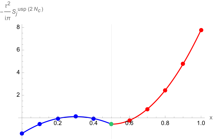
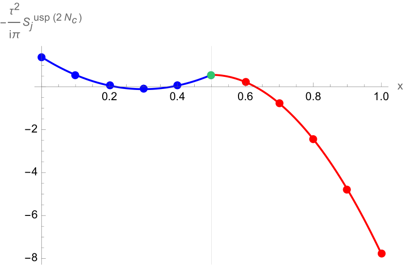
Figure 1: Behaviour of the saddle points for $usp(2N_{c})$ as $x\coloneqq j/N_{c}$ ranges from 0 to 1 and $N_{c}=10$. On the left: $\{\Delta_{a}\}=1/3$; on the right: $\{\Delta_{a}\}=2/3$.

3 The Cardy-like limit of the SCI of $\mathcal{N}\!=\!4$ of $so(2N_{c}+1)$ SYM

In this section we focus on the Cardy-like limit evaluation of the SCI for $4d$ $\mathcal{N}=4$ SYM with $so(2N_{c}+1)$ gauge algebra, determining the general structure of the saddle points. The index is given by

$$\begin{split}\mathcal{I}^{so(2N_{c}+1)}=&\frac{(p;p)_{\infty}^{N_{c}}(q;q)_{\infty}^{N_{c}}}{2^{N_{c}}N_{c}!}\prod_{a=1}^{3}\tilde{\Gamma}(\Delta_{a})^{N_{c}}\int\prod_{i=1}^{N_{c}}\mathrm{d}u_{i}\frac{\prod_{a=1}^{3}\prod_{i<j}\tilde{\Gamma}(\pm u_{ij}^{(\pm)}+\Delta_{a})}{\prod_{i<j}\tilde{\Gamma}(\pm u_{ij}^{(\pm)})}\cdot\\ &\cdot\frac{\prod_{a=1}^{3}\prod_{i=1}^{N_{c}}\tilde{\Gamma}(\pm u_{i}+\Delta_{a})}{\prod_{i=1}^{N_{c}}\tilde{\Gamma}(\pm u_{i})}.\end{split}$$ (22)

We define the effective action

$$\begin{split}S_{\mathrm{eff}}^{so(2N_{c}+1)}&=\sum_{a=1}^{3}\left(\sum_{i<j}\log\tilde{\Gamma}\left(\pm u_{ij}^{(\pm)}+\Delta_{a}\right)+\sum_{i=1}^{N_{c}}\log\tilde{\Gamma}\left(\pm u_{i}+\Delta_{a}\right)+N_{c}\log\tilde{\Gamma}\left(\Delta_{a}\right)\right)\\ &+\sum_{i<j}\log\theta_{0}\left(\pm u_{ij}^{(\pm)}\right)+\sum_{i=1}^{N_{c}}\log\theta_{0}\left(\pm u_{i}\right)+2N_{c}\log(p;p)_{\infty},\end{split}$$ (23)

such that the index is

$$\mathcal{I}^{so(2N_{c}+1)}=\frac{1}{{2^{N_{c}}N_{c}!}}\int\prod_{i=1}^{N_{c}}\mathrm{d}u_{i}\,e^{-S_{\mathrm{eff}}^{so(2N_{c}+1)}}$$ (24)

General solutions to the saddle point equations beyond the leading order Cardy-like limit can be found by first focusing on the leading term in the Cardy-like limit and then by expanding around those solutions accordingly, following the strategy of GonzalezLezcano:2020yeb . As $|\tau|\rightarrow 0$ the saddles will converge to the leading ones, capturing the full behaviour of the index up to exponentially suppressed terms in $|\tau|$.
The saddle point equations are

$$\begin{split}\sum_{a=1}^{3}\Bigg{[}\sum_{\begin{subarray}{c}j=1\\ j\neq k\end{subarray}}^{N_{c}}\bigg{(}\!B_{2}\{u_{ij}^{(\pm)}\!+\!\Delta_{a}\}\!-\!\!B_{2}\{-u_{ij}^{(\pm)}+\Delta_{a}\}\!\bigg{)}+B_{2}\{u_{i}+\Delta_{a}\}\!-\!B_{2}\{-u_{i}+\Delta_{a}\}\Bigg{]}\!=\!0.\end{split}$$ (25)

The absence of a factor 2 in the $\pm u_{i}$ roots of $so(2N_{c}+1)$ with respect to the ones of $usp(2N_{c})$ plays a crucial role in the behaviour of the structure of the saddles, leading to a rather different behaviour than the ones of the symplectic case, as showed in Figure 2 . We found that the solution with $N_{c}$ holonomies at zero, already studied in Amariti:2020jyx , lies inside a more general family of saddles parameterised by $L=0,N_{c}$, which counts the number of holonomies set to zero. The general saddle point is of the form $(L,N_{c}-L)$, with $L$ holonomies at zero and $N_{c}-L$ at $1/2$. As opposed to the symplectic case, there is no pairing between the $L$ and $L^{\prime}=N_{c}-L$ saddles.

Figure 2: Vacua distribution together with the corresponding group of the effective CS theory.

The saddle point beyond the leading order in the Cardy-like limit and the corresponding subleading contributions to the index are then obtained by expanding around the leading saddles.

3.1 $L$ holonomies at $u_{i}=0$, $K=N_{c}-L$ holonomies at $u_{i}=1/2$

We make the following ansatz for the general saddle point:

$$\hat{\mathbf{u}}=\begin{cases}\bar{u}_{j}=v_{j}\tau\hskip 136.5733ptj=1,...,L\\ \frac{1}{2}+\bar{u}_{L+r}\equiv\frac{1}{2}+\bar{w}_{r}=\frac{1}{2}+w_{r}\tau\hskip 28.45274ptr=1,...,K.\end{cases}$$ (26)

Then, expanding the effective action near $\hat{\mathbf{u}}$ for $|\tau|\rightarrow 0$ we obtain

$$S_{L,K}^{so(2N_{c}+1)}=-\frac{i\pi}{\tau^{2}}(2(L-K)-1)\eta_{1}+2K\eta_{2})\sum_{i=1}^{L}\bar{u}_{i}^{2}+\sum_{i<j}^{L}\log\left(2\sin\left(\frac{\pm\pi\bar{u}_{ij}^{(\pm)}}{\tau}\right)\right)+$$

$$+\sum_{i=1}^{L}\log\left(2\sin\left(\frac{\pm\pi\bar{u}_{i}}{\tau}\right)\right)-N_{c}\log(\tau)+$$

$$-\frac{i\pi}{\tau^{2}}((2(K-L)-3)\eta_{1}+(2L+1)\eta_{2})\sum_{r=1}^{K}\bar{w}_{r}^{2}+\sum_{r<s}^{K}\log\left(2\sin\left(\frac{\pm\pi\bar{w}_{rs}^{(\pm)}}{\tau}\right)\right)+$$

$$-\frac{i\pi}{\tau^{2}}\left(2(L-K)^{2}+L-3K\right)\prod_{a=1}^{3}\left(\{\Delta_{a}\}_{\tau}-\frac{1+\eta_{1}}{2}\right)$$

$$-\frac{i\pi}{2\tau^{2}}\left(K(1+2L)\right)\prod_{a=1}^{3}\left(\{2\Delta_{a}\}_{\tau}-\frac{1+\eta_{2}}{2}\right)+$$

$$+i\pi\left(\frac{(6-5\eta_{1})\left(2(L-K)^{2}+L-3K\right)}{12}+\frac{(12-5\eta_{2})K(1+2L)}{6}-N_{c}^{2}\right),$$ (27)

where again $\eta_{1}=\pm 1$ and $\eta_{2}=\pm 1$. The action (3.1) is manifestly not invariant under $L\leftrightarrow K$, differently to the symplectic case. Upon changing variables $\bar{u}_{j}=-i\sigma_{j}\tau$, we can read off the three sphere partition function a 3d pure CS theory. Such CS theories arise by expanding the holonomies around the $u_{i}=0$ and $u_{i}=1/2$ vacua, and they give rise to an odd and even rank orthogonal gauge group respectively. We obtain the partition function of an $s(o(2L+1)_{k_{1}}\times o(2K)_{k_{2}})$ pure CS theory with CS levels

$$\begin{cases}k_{1}=-(2(L-K)-1)\eta_{1}-2K\eta_{2}\\ k_{2}=-(2(K-L)-3)\eta_{1}-(2L+1)\eta_{2}\end{cases}$$ (28)

The index is then

$$\mathcal{I}=\sum_{L=0}^{N_{c}}\mathcal{I}_{L,N_{c}-L},\quad\text{where}\quad\mathcal{I}_{L,K}=\tau^{N_{c}}e^{-\frac{i\pi((2K-1)K+(2L+1)L)}{2}}\mathcal{I}_{0}Z_{S^{3}}^{s(o(2L+1)_{k_{1}}\times o(2K)_{k_{2}})}$$ (29)

and

$$\begin{split}\log\mathcal{I}_{0}&=-\frac{i\pi}{\tau^{2}}\left(2(L-K)^{2}+L-3K\right)\prod_{a=1}^{3}\left(\{\Delta_{a}\}_{\tau}-\frac{1+\eta_{1}}{2}\right)\\ &-\frac{i\pi}{2\tau^{2}}\left(K(1+2L)\right)\prod_{a=1}^{3}\left(\{2\Delta_{a}\}_{\tau}-\frac{1+\eta_{2}}{2}\right)-N_{c}\log(\tau)+\\ &+i\pi\left(\frac{(6-5\eta_{1})\left(2(L-K)^{2}+L-3K\right)}{12}+\frac{(12-5\eta_{2})K(1+2L)}{6}-N_{c}^{2}\right).\end{split}$$ (30)

3.2 General behaviour of the saddles

Again, the dominant saddle point in the Cardy-like limit depends on the region of chemical potentials we are in. To identify the leading saddle it is enough to focus on the leading order term. The behaviour of the saddles is determined by a second degree polynomial in $L\in[0,N_{c}]$.

$$\begin{split}-\frac{\tau^{2}}{i\pi}S_{L,N_{c}-L}^{so(2N_{c}+1)}=\left(2(N_{c}-2L)^{2}+4L-3N_{c}\right)\alpha_{1}+\frac{1}{2}\left((N_{c}-L)(1+2L)\right)\alpha_{2}.\end{split}$$ (31)

where $\alpha_{1,2}$ are defined in (19) The parabola has a vertex in

$$L=\frac{2N_{c}-1}{4}$$ (32)

independently of the chemical potentials.

Thus, it follows that the dominant saddle is either the one closer to the vertex with $L=\left\lfloor\frac{N_{c}}{2}\right\rfloor$, since $L$ must be integer, or the saddle with $L=N_{c}$ at the extremum of the domain of the parabola, depending on the region of chemical potentials we are considering. The saddle with $L=0$ is penalised, due to the vertex being closer to zero than to $N_{c}$; only in the large $N_{c}$ limit we expect to recover a pairing between the $L$ and the $L^{\prime}=N_{c}-L$ saddles as the symmetry axis of the parabola goes to $N_{c}/2$. In the “physical” regions we are in the M-wing or in the W-wing. In the first case the dominant saddle point is the one with $N_{c}$ holonomies at zero, while in the second case the dominant saddle is the one with $L=\left\lfloor\frac{N_{c}}{2}\right\rfloor$.

Summarizing, the M-wing is dominated by vanishing holonomies, while the saddle with $L=\left\lfloor\frac{N_{c}}{2}\right\rfloor$ holonomies at $u_{i}=0$ and the remaining at $u_{i}=1/2$ dominates the W-wing.

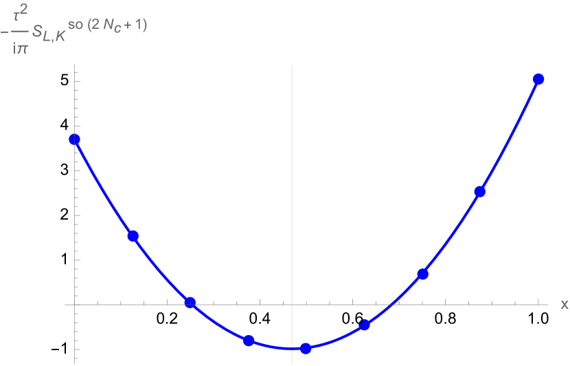
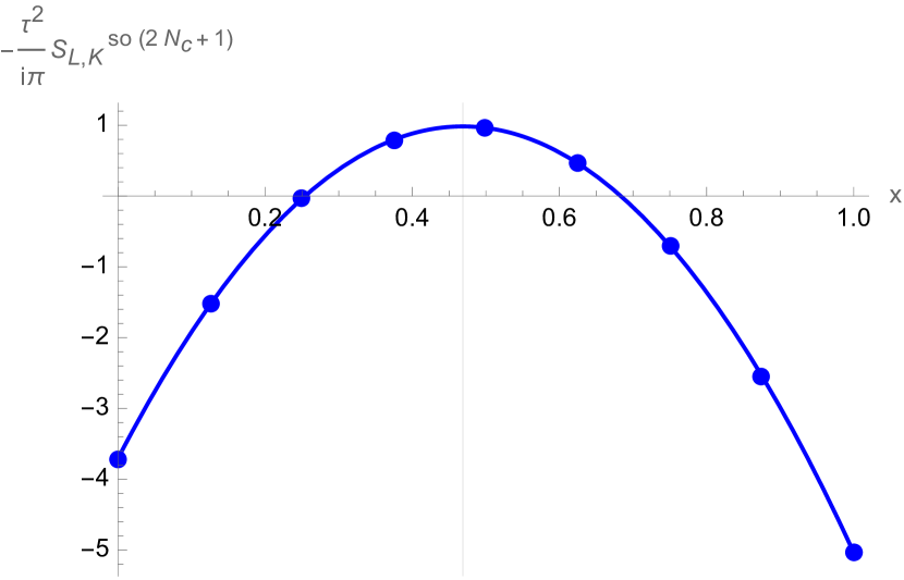
Figure 3: The behaviour of (31) as $x\coloneqq L/N_{c}$ ranges from 0 to 1. The vertical line passes through the vertex of the parabola. For presentation purposes we plotted the case with $N_{c}=8$. On the left: $\{\Delta_{a}\}=1/3$; on the right: $\{\Delta_{a}\}=2/3$.

4 S-duality

In this section we study the fate of 4d S-duality in the Cardy-like limit of the SCI. We start by matching the $1/|\tau|^{2}$ leading order contribution to the index when all the holonomies are vanishing in both the symplectic and orthogonal case. This saddle dominates the index in the M-wing of the potential and it reproduces the entropy function of the would be holographic dual black hole. Then we match the leading contributions in the region of parameter where the index is in the W-wing.

Then we consider the fate of S-duality also in presence of subleading contribution in $|\tau|$. As discussed above only few saddles survive for both $usp(2N_{c})$ and $so(2N_{c}+1)$. These saddles are exactly the ones that dominates the index in the M-wing and in the W-wing. In the case of the M-wing the full matching was discussed in Amariti:2020jyx . In the W-wing we show here that S-duality is preserved because of a non-trivial identity among the pure CS partition functions.

4.1 S-duality at the leading order

We begin our analysis by focusing on the leading $1/|\tau|^{2}$ order expansion of the index. The dominant contributions to the index in each region $\eta_{1}=-\eta_{2}=\mp 1$ have been identified in the previous sections and read

• M-wing ($\eta_{1}=-1$): the dominant contribution in the orthogonal case is achieved for vanishing holonomies. The symplectic theory is dominated by the same configuration of holonomies but the contribution is doubled due to the pairing between the saddles at $N_{c}$ holonomies at $u_{i}=0$ and at $N_{c}$ holonomies at $u_{i}=\frac{1}{2}$. As discussed in Amariti:2020jyx , the factor 2 degeneracy, understood as the presence of a $\mathbb{Z}_{2}$ global 1-form symmetry, is not apparent in the orthogonal theory at this order, for any finite $N_{c}$, and only once subleading corrections in $|\tau|$ are included such factor can be recovered.

• W-wing ($\eta_{1}=1$): The symplectic theory is dominated by the saddle point with $N_{c}$ holonomies at $u_{i}=\frac{1}{4}$, while for the orthogonal case the dominant contribution arise when $L=\lfloor\frac{N_{c}}{2}\rfloor$ holonomies sits at $u_{i}=0$ and the remaining ones at $u_{i}=\frac{1}{2}$.

At this level the expectation is that S-duality manifests as a matching between the dominant saddles. A natural question regards the role of the regions of chemical potentials. When an EFT interpretation of the underlying 3d pure CS theory is understood, the matching between the saddles is actually constrained by S-duality independently of the specific region of $\eta_{I}$ we sits in, because the topological sectors identified by the holonomies are equivalent. This is indeed the case for the saddle at vanishing holonomies for which an EFT interpretation for the CS terms can be recovered.

To be more explicit, one can readily observe that

$$\begin{split}\mathcal{I}_{N_{c},0}^{usp(2N_{c})}=\mathcal{I}_{N_{c},0}^{so(2N_{c}+1)}=\exp\left[-\frac{i\pi N_{c}(2N_{c}+1)}{\tau^{2}}\prod_{a=1}^{3}\left(\{\Delta_{a}\}-\frac{1+\eta_{1}}{2}\right)\right]\end{split}$$ (33)

which holds for any value of $\eta_{I}$ and it thus persists independently of the specific wing we are in.

Notice however that by sticking at order $1/|\tau|^{2}$ a proper matching can be achieved only considering the large $N_{c}$ limit, when the reflexive symmetry $L\leftrightarrow K$ between the saddles is recovered also in the orthogonal case. In fact, for $N_{c}\rightarrow\infty$ we get

$$\begin{split}&\mathcal{I}_{N_{c},0}^{usp(2N_{c})}+\mathcal{I}_{0,N_{c}}^{usp(2N_{c})}=\mathcal{I}_{N_{c},0}^{so(2N_{c}+1)}+\mathcal{I}_{0,N_{c}}^{so(2N_{c}+1)}=\\ =&\,2\exp\left[-\frac{i\pi N_{c}(2N_{c}+1)}{\tau^{2}}\prod_{a=1}^{3}\left(\{\Delta_{a}\}-\frac{1+\eta_{1}}{2}\right)\right]\end{split}$$ (34)

The same argument cannot be employed for the saddles dominating the W-wing as the EFT interpretation is less clear. However, also for these saddles the matching extends to any region of $\{\Delta_{a}\}$ at least for the leading order in $|\tau|$.

Indeed,

$$\mathcal{I}_{0,0,N_{c}}^{usp(2N_{c})}=\mathcal{I}_{\lfloor\frac{N_{c}}{2}\rfloor,\lceil\frac{N_{c}}{2}\rceil}^{so(2N_{c}+1)}=$$

$$=\exp\left[\frac{i\pi N_{c}}{\tau^{2}}\prod_{a=1}^{3}\left(\{\Delta_{a}\}-\frac{1+\eta_{1}}{2}\right)-\frac{i\pi(N_{c}^{2}+N_{c})}{4\tau^{2}}\prod_{a=1}^{3}\left(\{2\Delta_{a}\}-\frac{1+\eta_{2}}{2}\right)\right]$$ (35)

At this level of the discussion the fate of S-duality on the other saddles is unclear. Indeed we did not find a matching among the indices expanded around such saddles at leading order in $1/|\tau|^{2}$. The situation is clarified by taking into account the complete expansion in $|\tau|$, as we will show in the next sub-section.

4.2 Beyond the leading order

The 3d CS partition function on $S^{3}$ is

$$Z_{\mathfrak{g}}=\frac{1}{|W|}\int\prod_{i=1}^{\text{rk}\mathfrak{g}}d\sigma_{i}e^{\frac{i\pi k\sigma_{i}^{2}}{\omega_{1}\omega_{2}}}\prod_{\alpha(\sigma)}\Gamma_{h}^{-1}(\alpha(\sigma))$$ (36)

The exact evaluation of this partition function is already known in literature for algebras of type ABCD and it can be obtained by employing the Weyl character formula and its generalisations. As discussed before, the possible symmetry breaking patterns of the original gauge group for each holonomy configuration fall into an algebra of type ABCD. Therefore, we can get an explicit evaluation of the SCI on each saddle beyond the semiclassical expansion, with the most significant contribution coming from CS partition functions.

The explicit expression of such partition function for each algebra is presented in appendix C. All of them exhibits similar features. The general structure is

$$Z_{ABCD(m)_{k}}=\frac{\exp\left(i\pi f(m,k)\right)}{g(m,k)}\prod_{n\in I_{m}}2\sin(\pi\frac{n}{k})^{d(n)},$$ (37)

where $I_{m}$ is some subset of consecutive elements of (semi-)integers, typically depending on the rank $m$ of the group, $k$ is the CS level of the theory, while $f(m,k)$ and $g(m,k)$ are two functions depending on the details of $\mathfrak{g}$, with $g(m,k)$ such that $g(m,0)=0$, while $f(m,k)$ real, so that $\exp(i\pi f(m,k))$ is a phase. The function $d(n)$ represents a possible degeneracy, due to possible multiple occurrences of the same integer n.

A general consequence of (37) is that the level plays a crucial role in determining the physical relevance of the saddle point. First, for $k=0$ the TFT is not well defined. Second, when $k$ lies within $I_{m}$ the partition function is zero. The only case when (37) is non-vanishing is when $k>\mathrm{max}(I_{m})$.

Since the CS level is determined by the holonomy configuration of a chosen saddle, we can predict the stability and the contribution of such a saddle to the index only by studying the CS level for the emerging pure CS theories, expanding the effective action for the matrix model near such vacuum.

Focusing first on $\mathcal{N}=4$ $usp(2N_{c})$ SYM, the possible patterns of symmetry breaking found can be divided in two categories $usp(2N_{c})\rightarrow usp(2L)\times usp(2K)$ and $usp(2N_{c})\rightarrow usp(2L)\times usp(2L)\times su(K)\times u(1)$. For the first case, by inspecting (C) and remembering that the CS levels for the two pure CS theories are defined as in (13), we find that $Z^{usp(2(N_{c}-L))_{k_{2}}}=0$ when $0<L\leq\lfloor N_{c}/2\rfloor$. Moreover, under the reflexive symmetry $L\leftrightarrow N_{c}-L$ the role of $Z^{usp(2L)_{k_{1}}}$ and $Z^{usp(2(N_{c}-L)_{k_{2}})}$ is exchanged and we can conclude that $Z^{usp(2L)_{k_{1}}}=0$ when $\lfloor N_{c}/2\rfloor\leq L<N_{c}$. In addition, it can sporadically happen that the CS level is zero for some saddles with $L\neq 0,1/2$. Thus, beyond the semiclassical approximation the only non-vanishing saddle arising from the first family is the one with $N_{c}$ holonomies at $u_{i}=0$ together with its paired one with $N_{c}$ holonomies at $u_{i}=1/2$. All the other saddles give a vanishing partition functions and they are then perturbatively unstable.

The same argument can be applied to the second family of saddles leaving only one non-vanishing saddle with holonomy configuration defined by $N_{c}$ holonomies at $u_{i}=1/4$.

While the $1/|\tau|^{2}$ leading order calculation identifies such two saddles as the dominant contributions to the index, the analysis beyond the leading order shows that they are the only contributions to the index.

In addition, S-duality cannot hold without the explicit evaluation of the CS partition function obtained by a pertubation close to the saddle. This is because S-duality is expected to manifest in the Cardy-like limit as a matching between saddles of the two theories. Then, without an analysis of the subleading contributions in $|\tau|$ of each saddle to the index, not only there is not a clear understanding of the role played by the subleading saddles within the context of S-duality, but even a partial matching between the dominant ones cannot be achieved as discussed in Amariti:2020jyx .

The story proceeds in a similar way for the orthogonal $so(2N_{c}+1)$ case. In this case, we have just one family of saddles with $L$ holonomies at $u_{i}=0$ and $N_{c}-L$ at $u_{i}=1/2$, as discussed in Section 3. The original $so(2N_{c}+1)$ gauge algebra breaks into $s(o(2L+1)\times o(2(N_{c}-L)))$ and a $Z^{s(o(2L+1)_{k_{1}}\times o(2K)_{k_{2}})}$ factor (with $k_{1}$ and $k_{2}$ defined in (28)) appears in the evaluation of the subleading contributions in $|\tau|$ to the index in the Cardy-like limit.

Using the results presented in appendix C for the partition function of the CS gauge theories with orthogonal gauge algebra, together with (28) for the CS levels we find that the only non-vanishing saddles are the ones with either $N_{c}$ holonomies at zero or $L=\lfloor\frac{N_{c}}{2}\rfloor$ holonomies at $u_{i}=0$ and the remaining ones at $u_{i}=\frac{1}{2}$. These have been already identified as the dominant contributions to the index in the M-wing and W-wing respectively.

Summarising, S-duality predicts a matching between two pairs of saddles of the two theories, which must hold independently of the regions of charges that we are considering. In this sense also the distinction between the W and M shaped regions of the potential is unnecessary, because we have matched the whole expansions in $|\tau|$ in both the wings. The SCI for the two distinct 4d S-dual SYM theories reduces to

• $usp(2N_{c})$: $\mathcal{I}^{usp(2N_{c})}=2\mathcal{I}_{N_{c},0}+\mathcal{I}_{0,0,N_{c}}$.

• $so(2N_{c}+1)$: $\mathcal{I}^{so(2N_{c}+1)}=\mathcal{I}_{N_{c},0}+\mathcal{I}_{\lfloor\frac{N_{c}}{2}\rfloor,\lceil\frac{N_{c}}{2}\rceil}$.

The saddles with vanishing holonomies agree in the two theories, as already discussed in Amariti:2020jyx .

For both theories their contribution to the SCI is

$$\log\mathcal{I}_{N_{c},0}\sim-\frac{i\pi N_{c}(2N_{c}+1)}{\tau^{2}}\prod_{a=1}^{3}\left(\{\Delta_{a}\}_{\tau}-\frac{1+\eta_{1}}{2}\right)+\log 2.$$ (38)

This result holds thanks to the crucial role played by the evaluation of the CS partition function, responsible in the orthogonal case for the appearance of a $\log 2$, related to the $\log|G|$ correction to the black hole entropy, discussed in Amariti:2020jyx and understood as the presence of a 1-form symmetry.

It remains to show that the saddle with $N_{c}$ holonomies at $u_{i}=\frac{1}{4}$ of the $usp(2N_{c})$ theory agrees with the corresponding saddle with $L=\lfloor\frac{N_{c}}{2}\rfloor$ holonomies at $u_{i}=0$ and the remaining ones at $u_{i}=\frac{1}{2}$ of the $so(2N_{c}+1)$ theory.

In the symplectic theory the contribution of the saddle to the index is

$$\mathcal{I}_{N_{c},0}=\tau^{N}e^{-i\pi\frac{N_{c}^{2}}{2}}\mathcal{I}_{0}Z_{S^{3}}^{su(N_{c})_{h_{1}}}Z_{S^{3}}^{u(1)_{h_{2}}},$$ (39)

with

$$\begin{split}\log\mathcal{I}_{0}=&-\frac{i\pi N_{c}(N_{c}+1)}{4\tau^{2}}\prod_{a=1}^{3}\left(\{2\Delta_{a}\}_{\tau}-\frac{1+\eta_{2}}{2}\right)+\frac{i\pi N_{c}}{\tau^{2}}\prod_{a=1}^{3}\left(\{\Delta_{a}\}_{\tau}-\frac{1+\eta_{1}}{2}\right)\\ &+\frac{5i\pi N_{c}}{12}\left(\eta_{1}-(N_{c}+1)\eta_{2}\right)+\frac{i\pi N_{c}}{2}-N_{c}\log(\tau),\end{split}$$ (40)

For the orthogonal case the general expression (29) reduces to, when $L=\lfloor\frac{N_{c}}{2}\rfloor$,

$$\mathcal{I}_{\lfloor\frac{N_{c}}{2}\rfloor,\lceil\frac{N_{c}}{2}\rceil}=\tau^{N_{c}}e^{-\frac{i\pi N_{c}^{2}}{2}}\mathcal{I}_{0}Z_{S^{3}}^{s\left(o(2\lfloor\frac{N_{c}}{2}\rfloor+1)_{k_{1}}\times o(2\lceil\frac{N_{c}}{2}\rceil)_{k_{2}}\right)},$$ (41)

where

$$\begin{split}\log\mathcal{I}_{0}=&\frac{i\pi N_{c}}{\tau^{2}}\prod_{a=1}^{3}\left(\{\Delta_{a}\}_{\tau}-\frac{1+\eta_{1}}{2}\right)-\frac{i\pi N_{c}(N_{c}+1)}{4\tau^{2}}\prod_{a=1}^{3}\left(\{2\Delta_{a}\}_{\tau}-\frac{1+\eta_{2}}{2}\right)\\ &+\frac{5i\pi N_{c}}{12}\left(\eta_{1}-(N_{c}+1)\eta_{2}\right)+\frac{i\pi N_{c}}{2}-N_{c}\log(\tau)\end{split}$$ (42)

exactly matches the same term in the symplectic case.

Assuming S-duality is preserved, then a non-trivial integral identity between products of CS partition functions is expected. Thus, focusing on the regions where $\eta_{1}=-\eta_{2}=-1$ , it remains to show that

• $N_{c}=2m$:

  $$Z_{S^{3}}^{s(o(2m+1)_{2m+1}\times o(2m)_{2m+4})}=Z_{S^{3}}^{su(2m)_{2m+4}}Z_{S^{3}}^{u(1)_{4(2m+1)}}.$$ (43)

• $N_{c}=2m+1$:

  $$Z_{S^{3}}^{s(o(2m+2)_{2m+2}\times o(2m+1)_{2m+5})}=Z_{S^{3}}^{su(2m+1)_{2m+5}}Z_{S^{3}}^{u(1)_{4(2m+2)}}$$ (44)

It turns out that these identities indeed hold. The complete proof is presented in appendix D. At last, we achieved a matching between all the saddle points emerging in the Cardy-like limit of the SCI for $\mathcal{N}=4$ SYM theory with $usp(2N_{c})$ and $so(2N_{c}+1)$, thus recovering S-duality in the Cardy-like limit of the index for finite $N_{c}$.

To conclude the analysis we comment on the two special cases of $N_{c}=1$ and $N_{c}=2$, when the algebras isomorphisms between classical Lie algebras extend the matching between the saddle points to all the saddles of the two theories. We have

• When $N_{c}=1$, the isomorphism is made explicit upon changing variables in the SCI as $u^{so}=2v^{usp}$, implying $\mathcal{I}^{usp(2)}=\mathcal{I}^{so(3)}$. Accounting for the pairing degeneracy of the saddles with $v=0$ and $v=\frac{1}{2}$, we obtain the expected mapping between saddles:

  $$\begin{split}usp(2)&\hskip 28.45274ptso(3)\\ 0,\,1/2\hskip 2.84544pt&\longmapsto\hskip 8.5359pt0\\ 1/4\hskip 2.84544pt&\longmapsto\hskip 8.5359pt1/2.\end{split}$$ (45)

• The case of $N_{c}=2$ is physically more interesting, being the only case where a third matching between saddles of the two theories appears.

  Again, defining $u_{1,2}^{so}=v_{1}^{usp}\pm v_{2}^{usp}$, one can easily show that the two indices (1) and (22) can be mapped into each others. The corresponding mapping between the saddles in the two theories is the following:

  $$\begin{split}usp(4)&\hskip 28.45274ptso(5)\\ (0,0),(1/2,1/2)\hskip 5.69046pt&\longmapsto\hskip 8.5359pt(0,0)\\ (0,1/2)\hskip 5.69046pt&\longmapsto\hskip 8.5359pt(1/2,1/2)\\ (1/4,1/4)\hskip 5.69046pt&\longmapsto\hskip 8.5359pt(0,1/2).\end{split}$$ (46)

  Besides the two saddles, already discussed in full generality in the previous section, a third matching appears between the (0,1/2) saddle of $usp(4)$ and the (1/2,1/2) saddle of $so(5)$ as a consequence of the algebra isomorphism relating the two SCIs. However, the matching survives only at order $1/|\tau|^{2}$ in the Cardy-like expansion as, once the CS partition function contributions are included, an instability emerges in the two saddle points because the CS levels (13) and (28) vanish in this case.

5 Conclusions

In this paper we have studied the fate of S-duality in the Cardy like limit of the SCI of $\mathcal{N}=4$ SYM for the cases with gauge algebra $so(2N_{c}+1)$ and $usp(2N_{c})$. We have found that such duality is preserved (at finite $N_{c}$) in a non-trivial way and only after a complete analysis beyond the leading order $1/|\tau|^{2}$ in the Cardy-like limit. The calculation of the subleading corrections in $|\tau|$ requires a saddle point analysis, and, as we have shown here, there is a lower amount of saddles in the $so(2N_{c}+1)$ case with respect to the ones found in Amariti:2020jyx for $usp(2N_{c})$. While this is not a problem per se, because already at leading level in the W-wing, the index evaluated from two degenerate $usp(2N_{c})$ saddles coincides with the one evaluated on a single $so(2N_{c}+1)$, by evaluating only the leading contribution of each saddle in the Cardy-like limit we have not been able to fully match the index of $usp(2N_{c})$ with the one of $so(2N_{c}+1)$. Nevertheless we have matched the indices evaluated on the saddles that dominate in the M-wing and the indices evaluated on the saddles that dominate in the W-wing separately. Even if the matchings between these saddles holds at finite $N_{c}$, there can be also other saddles that contribute to the index. We have shown that in general these last never contribute to the SCI because the CS partition function generated from the expansion in $|\tau|$ vanishes for such saddles. We have eventually evaluated the CS partition functions and fully matched the index of the S-dual models in the Cardy-like limit.

Many open questions are leftover. First it should be interesting to study the fate of S-duality for models with less supersymmetry and multiple gauge groups. In principle we expect a that the behavior studied here applies to these cases as well and that similar conclusions can be reached.

Motivated by the study of cases with lower supersymmetry, another analysis that we did not perform here regards the study of the subleading corrections for $\mathcal{N}=4$ $so(2N_{c})$ SYM. Even if this is a self dual theory, understanding its behavior may be relevant for extending the analysis to models with $\mathcal{N}=1,2$, where also $so(2N_{c})$ gauge nodes can appear.

A further generalization regards the fate of Seiberg duality in models with four supercharges. In the toric case one can borrow the results of GonzalezLezcano:2020yeb , where the matching is indeed straightforward in the solutions denoted as “C-center”. Other solutions are nevertheless possible, as discussed in ArabiArdehali:2019orz , and it is relevant to understand if they are perturbatively stable, i.e. if they are not vanishing once the subleading terms and the CS actions are considered.

Partially related to the last issue, another consequence of our analysis regards the relation between the vacua of the $\mathcal{N}=1^{*}$ theory on the circle and the vacua extracted from the saddle point analysis of the SCI in the Cardy like limit. We have seen here that such correspondence does not seem to hold in the $usp(2N_{c})$ and $so(2N_{c}+1)$ cases, where the number of solutions does not grow with $N_{c}$ but it is fixed to $3$ in the first case and $2$ in the second case. As observed in Cassani:2021fyv this value is related to the presence of a 1-form global symmetry, and its value reflects the number of inequivalent lattices of charges of Wilson and ’t Hooft lines under the unbroken subgroup of the center of the gauge group. For example in the case of the C-center solutions for $SU(N_{c})/\mathbb{Z}_{C}$ $\mathcal{N}=4$ SYM such number is $N_{c}/C$. Furthermore this number corresponds to a logarithmic correction to the contribution of the degenerate saddle to the index. As discussed in Amariti:2020jyx , despite the different degeneration of the saddles, there is a matching of these logs in the index of $usp(2N_{c})$ and $so(2N_{c}+1)$ in the W-wing that emerges only after evaluating the CS partition function. In general it would be interesting if this behavior holds true in general, i.e.if the number of lattices associated to the same modding corresponds to the log corrections associated to the index.

To conclude, it is also tempting to associate, along the lines of Cassani:2021fyv ; ArabiArdehali:2021nsx , the results obtained here to a 3d effective action emerging from the integration over the massive KK modes coming from the matter multiplets in the reduction on the thermal $S^{1}$. While this interpretation is expected for the saddles at vanishing holonomies, it is less clear how to interpret our results for the other saddles along these lines. Indeed, even in absence of an EFT interpretation, following the discussion in ArabiArdehali:2021nsx (see also Cabo-Bizet:2021plf ), one can associate the saddles at non-vanishing holonomies to the expansion of the index with $e^{2\pi i\tau}$ approaches a root of unity. In the $su(N_{c})$ case the CS partition function corresponds to an orbifold partition functions on $S^{3}/\mathbb{Z}_{C}$. Furthermore such solutions are related to the orbifolds of the Euclidean AdS₅ BH Aharony:2021zkr . In our case such orbifold interpretation is not straightforward and it deserves further analysis.

Appendix A The superconformal index

In this appendix we survey the main definitions of the superconformal index that we have used in the paper. The index is defined as

$$\mathcal{I}\equiv\Tr(-1)^{F}e^{-\beta H}p^{J_{1}+\frac{R}{2}}q^{J_{2}+\frac{R}{2}}\prod_{f=1}^{\text{rk}\mathbf{F}}v_{f}^{q_{f}}$$ (47)

In this trace formula we $J_{i}$ are the angular momenta on the $S^{3}$, $R$ is the R-charge and $q_{f}$ are the flavor charges of the rank $\mathbf{F}$ flavor symmetry group $\mathfrak{f}$. The fugacities of these symmetries are denoted as $p,q$ and $v_{f}$ respectively. Instead of the trace formula it is useful to define the index for a gauge theory in terms of a matrix integral over the holonomies of the gauge algebra:

$$\mathcal{I}=\frac{(p;p)_{\infty}^{\text{rk}\mathfrak{g}}(q;q)_{\infty}^{\text{rk}\mathfrak{g}}}{|W_{\mathfrak{g}}|}\oint_{T^{\text{rk}\mathfrak{g}}}\prod_{i=1}^{\text{rk}\mathfrak{g}}\frac{dz_{i}}{2\pi iz_{i}}\frac{\prod_{a=1}^{n_{\chi}}\prod_{\rho_{a}}\Gamma_{e}((pq)^{{R_{a}}/{2}}z^{\rho_{\mathfrak{g}}^{a}}v^{\rho_{\mathfrak{f}}^{a}})}{\prod_{\alpha}\Gamma_{e}(z^{\alpha_{\mathfrak{g}}})}$$ (48)

where $\rho_{\mathfrak{g,f}}^{a}$ represent the weights for the chiral multiplet gauge and the flavor.

In the Cardy-like limit it is more convenient to work explicitly with the chemical potentials conjugated to the charges of the theory. Therefore we define

$$p\equiv e^{2\pi i\tau},\hskip 14.22636ptq\equiv e^{2\pi i\sigma},\hskip 14.22636ptv_{j}\equiv e^{2\pi i\xi_{j}},\hskip 14.22636ptz_{i}\equiv e^{2\pi iu_{i}}.$$ (49)

From 47 we can read off the chemical potential for the R-charge

$$\nu_{R}\equiv\frac{1}{2}(\tau+\sigma).$$ (50)

In the literature it is pretty common to encode all the charges associated with the global symmetries of the theory in a new set of fugacities $y_{a}$ together with the charges $\Delta_{a}$ defined by

$$y_{a}\equiv e^{2\pi i\Delta_{a}}\equiv((pq)^{{R_{a}}/{2}}v^{\rho_{\mathfrak{f}}^{a}}),$$ (51)

The charges $\Delta_{a}=\rho_{f}^{a}(\mathbf{\xi})+\nu_{R}R_{a}$ encode all the information about the flavour and R charges of the theory.

Appendix B Asymptotic formulas

In this appendix we collect the main formulas for the hypergeometric functions and their asymptotic expansions needed to perform a saddle-point evaluation of the SCI in the Cardy-like limit.

Let $\tau,\sigma\in\mathbb{H}$ and $p=e^{2\pi i\tau}$, $q=e^{2\pi i\sigma}$. The elliptic gamma function is defined as the infinite product

$$\Gamma_{e}(z;p,q)\equiv\Gamma_{e}(z)\coloneqq\prod_{i,j=0}^{\infty}\frac{1-p^{j+1}q^{k+1}/z}{1-zp^{j}q^{k}}.$$ (52)

We also define the modified elliptic gamma function as

$$\tilde{\Gamma}_{e}(u;\tau,\sigma)\equiv\tilde{\Gamma}_{e}(u)\coloneqq\Gamma_{e}(e^{2\pi iu};e^{2\pi i\tau},e^{2\pi i\sigma}).$$ (53)

The Pochhammer symbol is defined for complex $z,q$ with $|q|<1$ by

$$(z;q)_{\infty}\coloneqq\prod_{j=0}^{\infty}\left(1-zq^{k}\right).$$ (54)

We can then define the elliptic function $\theta_{0}$

$$\theta_{0}(u;\tau,\sigma)=(u;q)_{\infty}(q/u;q)_{\infty}=\prod_{j=0}^{\infty}\left(1-e^{2\pi i((j+1)\tau-u)}\right)\left(1-e^{2\pi i(u+j\tau)}\right)$$ (55)

and for our purposes it is enough to remember that it satisfies

$$\log\theta_{0}(u)=-\log\tilde{\Gamma}_{e}(u).$$ (56)

In the Cardy-like limit the asymptotic behaviour of these functions can be written introducing the $\tau-$modded value of a complex number:

$$\{u\}_{\tau}\equiv u-\lfloor\real(u)-\cot(\arg(\tau))\imaginary(u)\rfloor,$$ (57)

For $u\in\mathbb{R}$ it reduces to the ordinary fractional part $u-\lfloor u\rfloor$.

Writing $u\in\mathbb{C}$ as $u=\tilde{u}+\tau\check{u}$ with $\tilde{z},\check{z}\in\mathbb{R}$, the $\tau-$modded value satisfies

$$\{u\}_{\tau}=\{\tilde{u}\}+\tau\check{u},$$ (58)

Moreover from the definition it follows that

$$\{-u\}_{\tau}=\begin{cases}1-\{u\}_{\tau}\hskip 14.22636pt\tilde{u}\not\in\mathbb{Z}\\ -\{u\}_{\tau}\hskip 25.6073pt\tilde{u}\in\mathbb{Z}.\end{cases}$$ (59)

Then, as $|\tau|\rightarrow 0$ with $\Im{\tau}>0$ fixed, we have the following asymptotic behaviours

$$\log\left(q;q\right)_{\infty}\sim-\frac{i\pi}{12}\left(\frac{1}{\tau}+\tau\right)-\frac{1}{2}\log(-i\tau)+\mathcal{O}\left(e^{\frac{2\pi\sin{\arg(\tau)}}{|\tau|}}\right),$$ (60)

$$\begin{split}\log\theta_{0}(u;\tau)\sim&\frac{i\pi}{\tau}\{u\}_{\tau}(1-\{u\}_{\tau})+i\pi\{u\}_{\tau}-\frac{i\pi}{6\tau}\left(1+3\tau+\tau^{2}\right)+\\ &+\log\left[\left(1-e^{-\frac{2\pi i}{\tau}\{u\}_{\tau}}\right)\left(1-e^{-\frac{2\pi i}{\tau}(1-\{u\}_{\tau})}\right)\right]+\mathcal{O}\left(e^{\frac{2\pi\sin{\arg(\tau)}}{|\tau|}}\right),\end{split}$$ (61)

$$\log\tilde{\Gamma}(u;\tau)\sim 2\pi iQ(\{u\}_{\tau};\tau)+\mathcal{O}\left(|\tau|^{-1}e^{\frac{2\pi\sin{\arg(\tau)}}{|\tau|}\min(\{u\}_{\tau},1-\{u\}_{\tau})}\right),$$ (62)

provided that $\tilde{u}\not\in\mathbb{Z}$, with $Q(u)$ defined as

$$Q(u;\tau)=-\frac{B_{3}(u)}{6\tau^{2}}+\frac{B_{2}(u)}{2\tau}-\frac{5B_{1}(u)}{12}+\frac{\tau}{12},$$ (63)

where $B_{n}(u)$ are the Bernoulli polynomials

$$B_{1}(u)=u-\frac{1}{2},\hskip 28.45274ptB_{2}(u)=u^{2}-u+\frac{1}{6},\hskip 28.45274ptB_{3}(u)=u^{3}-\frac{3}{2}u^{2}+\frac{u}{2}.$$ (64)

The Bernoulli polynomials (and their modded version $B(\{x\}_{\tau})$) satisfy the following identity, known as Raabe’s formula

$$\sum_{J=0}^{C-1}B_{n}\left(\frac{J}{C}+u\right)=\frac{1}{C^{n-1}}B_{n}\left(Cu\right),$$ (65)

through which we expressed the effective actions in terms of products of $\{C\Delta\}_{\tau}$ terms, with $C=1,2,4$.

Appendix C $Z_{S^{3}}$ for pure 3d $\mathcal{N}=2$ CS theories with ABCD gauge algebra

In this appendix we collect some useful formulas on the exact evaluation of the 3d partition function of the three sphere partition function 3d of pure CS gauge theories with gauge algebra $\mathfrak{g}$ of ABCD type. The integral formula corresponds to a matrix integral of the form

$$Z_{\mathfrak{g}}=\frac{1}{|W|}\int\prod_{i=1}^{\text{rk}\mathfrak{g}}d\sigma_{i}e^{\frac{i\pi k\sigma_{i}^{2}}{\omega_{1}\omega_{2}}}\prod_{\alpha(\sigma)}\Gamma_{h}^{-1}(\alpha(\sigma))$$ (66)

where $\alpha(\sigma)$ represent the simple roots of the algebra and $\Gamma_{h}$ are hyperbolic gamma functions

$$\Gamma_{h}(z)\equiv\prod_{m,n=1}^{\infty}\frac{(n+1)\omega_{1}+(m+1)\omega_{2}-z}{n\omega_{1}+m\omega_{2}}$$ (67)

Expression (66) can be rewritten in terms of hyperbolic sines, as in the main text, by employing the following property of the hyperbolic gamma functions

$$\frac{1}{\Gamma_{h}(x)\Gamma_{h}(-x)}=-4\sin(\frac{\pi x}{\omega_{1}})\sin(\frac{\pi x}{\omega_{2}}).$$ (68)

We have observed in the body of the paper that the Cardy-like limit of the SCI gives rise (for charges $\Delta_{a}\neq 0,2$) to a matrix integral of the type (66) for pure CS gauge algebras of $\mathfrak{g}$ of ABCD type.

Such partition functions can be exactly evaluated and the results have already been obtained in the literature. Here we collect these results, because the exact evaluations of $Z_{\mathfrak{g}}$ has allowed us to perform the precision checks on S-duality. Furthermore we restrict to the case of $S^{3}$, setting $\omega_{1}=\omega_{2}$ because we have studied the case with collinear angular momenta in the body of the paper.

Let us start surveying the various results. The evaluation of the partition function for pure CS $\mathfrak{g}=u(N_{c})$ at level $k$ was performed in Kapustin:2009kz . The final formula is

$$Z_{u(N_{c})_{k}}= \ \frac{e^{\frac{i\pi N_{c}\left(3kN_{c}-2N_{c}^{2}-6k+2\right)}{12k}}}{k^{\frac{N_{c}}{2}}}\prod_{m=1}^{N_{c}-1}\left(2\sin\left(\frac{\pi m}{k}\right)\right)^{N_{c}-m}$$ (69)

It is also possible to relate the $u(N_{c})$ case to the $su(N_{c})$ one, thanks to the formula

$$Z_{su(N_{c})_{k}}= \ \sqrt{\frac{k}{iN_{c}}}Z_{u(N_{c})_{k}}$$ (70)

Such distinction is important in our analysis, because we often deal with $su(N_{c})\times U(1)$ gauge theories, with different CS level for the abelian factor.

The partition function for 3d pure CS on $S^{3}$ with $\mathfrak{g}=usp(2N_{c})$ at level $k$ is VanDeBult

$$Z^{usp(2N_{c})_{k}}= \ \frac{\exp\left(-\frac{i\pi N_{c}(2+6N_{c}+4N_{c}^{2}+6k+3|k|)}{12k}\right)}{(2|k|)^{\frac{N_{c}}{2}}}\cdot$$

$$\cdot\!\!\!\!\prod_{1\leq j<\ell\leq N_{c}}4\sin\left(\frac{\pi(j+\ell)}{2k}\right)\sin\left(\frac{\pi(j-\ell)}{2k}\right)\prod_{j=1}^{N_{c}}2\sin\left(\frac{\pi j}{k}\right)\quad.$$ (71)

To conclude.the survey we consider the orthogonal cases, studied in Amariti:2020jyx . The case of $\mathfrak{g}=so(2N_{c}+1)$ at level $k$ gives

$$Z^{so(2N_{c}+1)_{k}}= \ \frac{\exp\left(\frac{i\pi N_{c}\left(12kN_{c}-8N_{c}^{2}-9|k|+2\right)}{12k}\right)}{|k|^{\frac{N_{c}}{2}}}\cdot$$

$$\cdot\!\!\!\!\prod_{1\leq j<\ell\leq N_{c}}4\sin\left(\frac{\pi(j+\ell-1)}{k}\right)\sin\left(\frac{\pi(j-\ell)}{k}\right)\prod_{j=1}^{N_{c}}2\sin\left(\frac{\pi(2j-1)}{2k}\right)\,$$ (72)

while for of $\mathfrak{g}=so(2N_{c})$ at level $k$ we have

$$Z^{so(2N_{c})_{k}}_{S_{b}^{3}}= \ \frac{\exp\left(\frac{i\pi N_{c}\left(12kN_{c}-8N_{c}^{2}-9|k|+2\right)}{12k}\right)}{|k|^{\frac{N_{c}}{2}}}\cdot$$

$$\cdot\prod_{1\leq j<\ell<N_{c}}4\sin\left(\frac{\pi(j+\ell-2}{|k|}\right)\sin\left(\frac{\pi(j-\ell)}{|k|}\right)\ .$$ (73)

Appendix D Proof of (43)

In this appendix we prove the relation (43) between the partition functions of pure CS gauge theories that we have used in the body of the paper in order to show how S-duality is preserved in the Cardy-like limit in the region where the index is dominated by the $W$-wing shaped potential. As discussed in the paper we have identified two different possibilities for the $usp(2N_{c})/so(2N_{c}+1)$ duality, depending on the parity of $N_{c}$. For $N_{c}=2m$ the expected relation is (43) that we reproduce here for the ease of the reader

$$Z_{S(O(2m+1)_{2m+1}\times O(2m)_{2m+4})}=Z_{U(2m)_{2m+4,4(2m+1)}}$$ (74)

while for $N_{c}=2m+1$ the expected relation is (44)

$$Z_{S(O(2m+2)_{2m+2}\times O(2m+1)_{2m+5})}=Z_{U(2m+1)_{2m+5,4(2m+2)}}$$ (75)

Two comments are in order. First the normalization of the $U(1)$ factor follows the conventions of appendix A of Amariti:2020xqm . Second, the partition function for the orthogonal case has been denoted here as schematically as $S(O(n)\times O(m))$ but it coincides with the one of $so(n)\times O(m)$ and $O(n)\times so(m)$.

The two identities (74). and (75) can be shown explicitly. In the following we give a direct derivation of (74). An analogous derivation holds for (75).

We start observing that the partition function $Z_{so(2m+1)_{2m+1}}$ can be evaluated, inferring the results from the evaluation of $Z_{so(2n+1)_{2n-1}}$ given in Amariti:2020jyx . We have

$$Z_{so(2m+1)_{2m+1}}=\frac{e^{\frac{1}{12}i\pi m(2m-1)}}{\sqrt{2m+1}}$$ (76)

On the other hand we can estimate the relation between the products of trigonometric functions that are inside the $so(2m)$ and the $U(2m)$ partition functions. They are

$$\mathcal{P}_{SO}\equiv\prod_{p=1}^{m}\prod_{q=p+1}^{m}4\sin\left(\frac{\pi(p-q)}{2(m+2)}\right)\sin\left(\frac{\pi(p+q-2)}{2(m+2)}\right)$$ (77)

and

$$\mathcal{P}_{SU}\equiv\prod_{p=1}^{2m-1}\left(2\sin\left(\frac{\pi p}{2m+4}\right)\right)^{2m-p}=\prod_{p=1}^{2m}\prod_{q=p+1}^{2m}2\sin\left(\frac{\pi(p-q)}{m+4}\right)$$ (78)

respectively

The ratio between such quantities can be simplified by using the partition functions of the pure 3d $\mathcal{N}=2$ CS $U(n)_{n}$ and $so(2n)_{2(n-1)}$ theories. They first one can be read from Amariti:2020jyx and for $Z_{so(2m+6)_{2(m+2)}}$ it gives

$$\prod_{p=1}^{m+3}\prod_{q=p+1}^{m+3}4\sin\left(\frac{\pi(p-q)}{2(m+2)}\right)\sin\left(\frac{\pi(p+q-2)}{2(m+2)}\right)=2e^{\frac{1}{2}i\pi\left(m^{2}+m+2\right)}(2m+4)^{\frac{m+3}{2}}$$ (79)

while the second one, for $Z_{U(m+4)_{m+4}}$, can be read from Kapustin:2009kz and it gives

$$\prod_{p=1}^{2m+4}\prod_{q=p+1}^{2m+4}2\sin\left(\frac{\pi(p-q)}{2m+4}\right)=(2m+4)^{m+2}$$ (80)

Using (79) we simplify (77) as

$$\mathcal{P}_{SO}=2e^{\frac{1}{2}i\pi\left(m^{2}+m+2\right)}(2m+4)^{\frac{m+3}{2}}\Theta_{SO}$$ (81)

with

$$\Theta_{SO} = \frac{1}{\prod_{p=1}^{m}\prod_{q=m+1}^{m+3}4\sin\left(\frac{\pi(p-q)}{2(m+2)}\right)\sin\left(\frac{\pi(p+q-2)}{2(m+2)}\right)}$$ (82)

$$\times \frac{1}{\prod_{p=m+1}^{m+2}\prod_{q=p}^{m+3}4\sin\left(\frac{\pi(p-q)}{2(m+2)}\right)\sin\left(\frac{\pi(p+q-2)}{2(m+2)}\right)}$$

Using (80) we simplify (78) as

$$\mathcal{P}_{SU}=(2m+4)^{m+2}\Theta_{SU}$$ (83)

with

$$\Theta_{SU}=\frac{1}{\prod_{p=1}^{2m}\prod_{q=2m+1}^{2m+4}2\sin\left(\frac{\pi(p-q)}{2m+4}\right)\cdot\prod_{p=2m+1}^{2m+3}\prod_{q=p+1}^{2m+4}2\sin\left(\frac{\pi(p-q)}{2m+4}\right)}$$ (84)

Next we want to show that

$$\frac{\Theta_{SU}}{\Theta_{SO}}=\frac{(-1)^{m+1}}{m+2}$$ (85)

In order to evaluate this ratio we start observing that

$$\frac{\prod_{p=m+1}^{m+2}\prod_{q=p}^{m+3}4\sin\left(\frac{\pi(p-q)}{2(m+2)}\right)\sin\left(\frac{\pi(p+q-2)}{2(m+2)}\right)}{\prod_{p=2m+1}^{2m+3}\prod_{q=p+1}^{2m+4}2\sin\left(\frac{\pi(p-q)}{2m+4}\right)}=-1$$ (86)

We are then left then with

$$\frac{\Theta_{SU}}{\Theta_{SO}} = -\frac{\prod_{p=1}^{m}\prod_{q=m+1}^{m+3}4\sin\left(\frac{\pi(p-q)}{2(m+2)}\right)\sin\left(\frac{\pi(p+q-2)}{2(m+2)}\right)}{\prod_{p=1}^{2m}\prod_{q=2m+1}^{2m+4}2\sin\left(\frac{\pi(p-q)}{2m+4}\right)}$$ (87)

$$= \frac{(-1)^{m+1}}{\sin\left(\frac{4\pi}{2m+4}\right)\cdot\prod_{p=1}^{m}2\sin\left(\frac{\pi(p+1)}{2m+4}\right)\cdot\prod_{p=1}^{m-1}2\sin\left(\frac{\pi p}{2m+4}\right)}$$

In order to conclude the proof of (85) we need to estimate the denominator of (87). This can be done by using the relations

$$\sin\left(\frac{4\pi}{2m+4}\right)=4\sin\left(\frac{\pi(2m+3)}{2(m+2)}\right)\sin\left(\frac{\pi(m+3)}{2(m+2)}\right)\sin\left(\frac{\pi(m+4)}{2(m+2)}\right)$$ (88)

and

$$\prod_{p=1}^{m}\sin\left(\frac{\pi(p+1)}{2(m+2)}\right)=\prod_{p=m+3}^{2m+2}\sin\left(\frac{\pi p}{2(m+2)}\right)$$ (89)

Such that the denominator of (87) becomes

$$\frac{1}{2}\prod_{p=1}^{2m+3}2\sin\left(\frac{\pi p}{2m+4}\right)=m+2$$ (90)

Then by plugging this result in (87) we arrive at (85). Eventually we plug (76) and (85) in (74) such to verify the latter.

To conclude we have not presented the explicit derivation of (75), because it can be derived along the same lines of the analysis performed in this appendix.

References

• (1) J. B. Gutowski and H. S. Reall, General supersymmetric AdS(5) black holes, JHEP 04 (2004) 048 [hep-th/0401129].
• (2) J. B. Gutowski and H. S. Reall, Supersymmetric AdS(5) black holes, JHEP 02 (2004) 006 [hep-th/0401042].
• (3) S. M. Hosseini, K. Hristov and A. Zaffaroni, An extremization principle for the entropy of rotating BPS black holes in AdS5, JHEP 07 (2017) 106 [1705.05383].
• (4) S. Choi, J. Kim, S. Kim and J. Nahmgoong, Large AdS black holes from QFT, 1810.12067.
• (5) F. Benini and E. Milan, Black Holes in 4D $\mathcal{N}$=4 Super-Yang-Mills Field Theory, Phys. Rev. X 10 (2020) 021037 [1812.09613].
• (6) C. Romelsberger, Counting chiral primaries in N = 1, d=4 superconformal field theories, Nucl. Phys. B 747 (2006) 329 [hep-th/0510060].
• (7) J. Kinney, J. M. Maldacena, S. Minwalla and S. Raju, An Index for 4 dimensional super conformal theories, Commun. Math. Phys. 275 (2007) 209 [hep-th/0510251].
• (8) M. Honda, Quantum Black Hole Entropy from 4d Supersymmetric Cardy formula, Phys. Rev. D 100 (2019) 026008 [1901.08091].
• (9) A. Arabi Ardehali, Cardy-like asymptotics of the 4d $\mathcal{N}=4$ index and AdS5 blackholes, JHEP 06 (2019) 134 [1902.06619].
• (10) J. Kim, S. Kim and J. Song, A 4d $\mathcal{N}$ = 1 Cardy Formula, JHEP 01 (2021) 025 [1904.03455].
• (11) A. Cabo-Bizet, D. Cassani, D. Martelli and S. Murthy, The asymptotic growth of states of the 4d $\mathcal{N}=1$ superconformal index, JHEP 08 (2019) 120 [1904.05865].
• (12) A. Amariti, I. Garozzo and G. Lo Monaco, Entropy function from toric geometry, Nucl. Phys. B 973 (2021) 115571 [1904.10009].
• (13) A. González Lezcano and L. A. Pando Zayas, Microstate counting via Bethe Ansätze in the 4d $\mathcal{N}$ = 1 superconformal index, JHEP 03 (2020) 088 [1907.12841].
• (14) A. Lanir, A. Nedelin and O. Sela, Black hole entropy function for toric theories via Bethe Ansatz, JHEP 04 (2020) 091 [1908.01737].
• (15) A. Cabo-Bizet and S. Murthy, Supersymmetric phases of 4d $\mathcal{N}$ = 4 SYM at large $N$, JHEP 09 (2020) 184 [1909.09597].
• (16) A. Arabi Ardehali, J. Hong and J. T. Liu, Asymptotic growth of the 4d $\mathcal{N}$ = 4 index and partially deconfined phases, JHEP 07 (2020) 073 [1912.04169].
• (17) S. Murthy, The growth of the $\frac{1}{16}$-BPS index in 4d $\mathcal{N}=4$ SYM, 2005.10843.
• (18) A. Cabo-Bizet, D. Cassani, D. Martelli and S. Murthy, The large-$N$ limit of the 4d $\mathcal{N}$ = 1 superconformal index, JHEP 11 (2020) 150 [2005.10654].
• (19) P. Agarwal, S. Choi, J. Kim, S. Kim and J. Nahmgoong, AdS black holes and finite N indices, Phys. Rev. D 103 (2021) 126006 [2005.11240].
• (20) F. Benini, E. Colombo, S. Soltani, A. Zaffaroni and Z. Zhang, Superconformal indices at large $N$ and the entropy of AdS5 $\times$ SE5 black holes, Class. Quant. Grav. 37 (2020) 215021 [2005.12308].
• (21) A. Cabo-Bizet, From multi-gravitons to Black holes: The role of complex saddles, 2012.04815.
• (22) A. González Lezcano, J. Hong, J. T. Liu and L. A. Pando Zayas, Sub-leading Structures in Superconformal Indices: Subdominant Saddles and Logarithmic Contributions, JHEP 01 (2021) 001 [2007.12604].
• (23) A. Amariti, M. Fazzi and A. Segati, The SCI of $\mathcal{N}$ = 4 USp(2Nc) and SO(Nc) SYM as a matrix integral, JHEP 06 (2021) 132 [2012.15208].
• (24) A. Amariti, M. Fazzi and A. Segati, Expanding on the Cardy-like limit of the SCI of 4d $\mathcal{N}$ = 1 ABCD SCFTs, JHEP 07 (2021) 141 [2103.15853].
• (25) O. Aharony, F. Benini, O. Mamroud and E. Milan, A gravity interpretation for the Bethe Ansatz expansion of the $\mathcal{N}=4$ SYM index, Phys. Rev. D 104 (2021) 086026 [2104.13932].
• (26) E. Colombo, The large-N limit of 4d superconformal indices for general BPS charges, JHEP 12 (2022) 013 [2110.01911].
• (27) S. Choi, S. Jeong, S. Kim and E. Lee, Exact QFT duals of AdS black holes, 2111.10720.
• (28) A. Cabo-Bizet, On the 4d superconformal index near roots of unity: bulk and localized contributions, JHEP 02 (2023) 134 [2111.14941].
• (29) S. Murthy, Unitary matrix models, free fermions, and the giant graviton expansion, Pure Appl. Math. Quart. 19 (2023) 299 [2202.06897].
• (30) J. Boruch, M. T. Heydeman, L. V. Iliesiu and G. J. Turiaci, BPS and near-BPS black holes in $AdS_{5}$ and their spectrum in $\mathcal{N}=4$ SYM, 2203.01331.
• (31) O. Mamroud, The SUSY Index Beyond the Cardy Limit, 2212.11925.
• (32) D. Cassani and Z. Komargodski, EFT and the SUSY Index on the 2nd Sheet, SciPost Phys. 11 (2021) 004 [2104.01464].
• (33) A. Arabi Ardehali and S. Murthy, The 4d superconformal index near roots of unity and 3d Chern-Simons theory, JHEP 10 (2021) 207 [2104.02051].
• (34) L. Di Pietro and Z. Komargodski, Cardy formulae for SUSY theories in $d=$ 4 and $d=$ 6, JHEP 12 (2014) 031 [1407.6061].
• (35) O. Aharony, S. S. Razamat, N. Seiberg and B. Willett, 3d dualities from 4d dualities, JHEP 07 (2013) 149 [1305.3924].
• (36) A. A. Ardehali and J. Hong, Decomposition of BPS moduli spaces and asymptotics of supersymmetric partition functions, JHEP 01 (2022) 062 [2110.01538].
• (37) A. Kapustin, B. Willett and I. Yaakov, Exact Results for Wilson Loops in Superconformal Chern-Simons Theories with Matter, JHEP 03 (2010) 089 [0909.4559].
• (38) F. van de Bult, Hyperbolic Hypergeometric Functions, http://www.its.caltech.edu/ vdbult/Thesis.pdf, Thesis (2008) .
• (39) A. Amariti and M. Fazzi, Dualities for three-dimensional $\mathcal{N}=2$ $SU(N_{c})$ chiral adjoint SQCD, JHEP 11 (2020) 030 [2007.01323].