Steering Control of an Autonomous Unicycle

Abstract

The steering control of an autonomous unicycle is considered. The underlying dynamical model of a single rolling wheel is discussed regarding the steady state motions and their stability. The unicycle model is introduced as the simplest possible extension of the rolling wheel where the location of the center of gravity is controlled. With the help of the Appellian approach, a state space representation of the controlled nonholonomic system is built in a way that the most compact nonlinear equations of motions are constructed. Based on controllability analysis, feedback controllers are designed which successfully carry out lane changing and turning maneuvers. The behavior of the closed-loop system is demonstrated by numerical simulations.

I Introduction

Micro-mobility solutions are spreading rapidly in urban environments [1]. Among these, human-ridden electric unicycles (EUCs) become more and more popular transportation devices; see Figure 1(a). These micro-mobility vehicles can match the speed of automobiles in urban traffic while their compact size make them appealing for commute in congested environments. Due to the three dimensional spatial rolling of the wheel and the stabilization of an unstable equilibrium, the unique dynamics of the unicycle combines agility and maneuverability. To exploit these properties, one may consider making EUCs autonomous (see Figure 1(b)) which opens up an challenging avenue for modeling, dynamics and control.

During the last few decades, several autonomous unicycle designs have appeared in the literature which differ on various aspects such as the number and/or types of actuators that can be used to control the dynamics. The first publication related to autonomous unicycles known to the authors is [2] in which the longitudinal/pitch motion is controlled by balancing an inverted pendulum, and the lateral/tilt motion is controlled by moving a mass perpendicular to the wheel. Two other approaches are presented in [3]. In the first case, the longitudinal/pitch motion is also controlled by balancing an inverted pendulum, while the turning/yaw motion of the unicycle is controlled by an overhead flywheel. In the second case, the tilt is controlled by adding a second pendulum swinging in the lateral plane. The overhead flywheel approach was further explored in [4, 5]; the lateral pendulum approach can be found in [6]. Instead of a point mass or lateral pendulum, the tilt motion of the unicycle can also be controlled by a lateral flywheel, see, for example, [7, 8, 9], while the combination of overhead and lateral flywheels can be found in [10, 11]. Furthermore, the application of gyroscopes for lateral stabilization and steering is presented in [12, 13, 14, 15]. Humanoid-type autonomous unicycles are introduced and analyzed in [16, 17]. Most of these approaches provide satisfactory dynamic behavior. However, their complexity prohibits closed-form analysis of the control system, while human operators control these vehicles in a seemingly simple way.

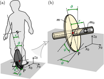
Figure 1: Riding an EUC (a), and an analogous autonomous system (b).

The rolling of the wheel is described by kinematic constraints in the most compact form [18, 19, 20, 21]. Thus, the unicycle can be considered as a nonholonomic mechanical system. Such systems are often described by the generalized Lagrangian equations (or Routh–Voss equations) [22, 23], and this method yields in a differential-algebraic system of equations which has its own challenges. Instead, the Appellian approach [24, 25], which is used in this study, results in a system of first order ordinary differential equations as the most compact and simplest representation of the underlying nonholonomic system. Apart from its simplicity, the Appellian approach yields a control affine system, with the internal forces and/or torques acting as control inputs, and thus, the resulting nonlinear dynamical model is ready for control design. This enables one to deploy a plethora of control techniques without dealing with the complexity of differential-algebraic systems. More details about nonholonomic systems may be found in [26, 27, 28, 29, 30, 31, 32, 33].

In this study, a new autonomous unicycle model consisting of a wheel and a moving mass (see Figure 1(b)) is proposed. The tilt and yaw motions are controlled via moving the mass along the axle. This provides the simplest possible representation for unicycle control and enables us to analyze stability and controllability of different motions analytically. First, by omitting the moving mass, we explore the dynamics of the uncontrolled rolling and categorize different steady state motions (e.g., straight rolling, turning) of interest. This simplified case also enables us to explain the self stabilizing effects in the tilt direction above a critical speed. By adding the moving mass and an internal force between the wheel and and the mass, we create a control system and study how the steady states are affected. Moreover, this enables us to design feedback controllers which stabilize the steady states at any speed and enables the unicycle to perform a large variety of maneuvers including lane changes and sharp turns. Our control design exploits the inherent instabilities of the system in order to demonstrate high level of maneuverability.

The article is structured as follows. In Section II, the modeling framework and steady state analysis of the rolling wheel example are presented. Section III introduces a novel autonomous unicycle model and analyzes the steady states of the open-loop system. Section IV proposes controller designs that successfully perform lane changing and turning maneuvers. The performance of these controllers are demonstrated by numerical simulations. We conclude our results in Section V and provide future research directions.

II Dynamics of the rolling wheel

We introduce the modeling framework and notation on the rolling wheel example which represents the uncontrolled behavior of the unicycle. We reveal the dynamical characteristics, including the self-stabilization phenomenon, which can be exploited for control design.

II-A Governing equations

A wheel has ${N=6}$ degrees of freedom (DoF) in the three dimensional space. That is, the spatial position and orientation are described by six variables: the position of the center of gravity ${\mathbf{r}_{\rm G}=[x_{\rm G}\,\ y_{\rm G}\,\ z_{\rm G}]^{\mathsf{T}}}$ and the yaw ($\psi$), tilt ($\vartheta$) and pitch ($\varphi$) angles; see Figure 2. Note that tilt is often called roll in the vehicle dynamics literature but here we do not use this convention to avoid confusion with the fact that disc rolls on the horizontal plane.

To describe the motion of the wheel, three coordinate frames are introduced: see Figure 2. The axes $x_{0}$ and $y_{0}$ of the ground fixed frame ${\mathrm{F}_{0}}$ span the horizontal plane and its $z_{0}$ axis gives the vertical direction. The frame ${\mathrm{F}_{1}}$ is moving with the wheel such that its origin is the wheel-ground contact point P. This frame is rotated with respect to ${\mathrm{F}_{0}}$ around the $z_{0}$ axis with yaw angle $\psi$ so that the $x_{1}$ axis is tangential to the path of P (the fixed polode). The frame ${\mathrm{F}_{2}}$ is rotated with respect to ${\mathrm{F}_{1}}$ around the $x_{1}$ axis with the tilt angle $\vartheta$ so the $x_{1}$ and $z_{1}$ axes span the plane of the wheel and the $y_{2}$ axis is aligned with the wheel axle. The origin of frame ${\mathrm{F}_{2}}$ is placed to the wheel center point $\mathrm{G}$.

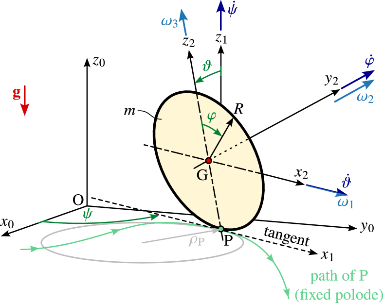
Figure 2: Mechanical model of the rolling wheel

Assume that the wheel rolls without slipping; the kinematic condition of rolling is that the instantaneous center of rotation coincides with the contact point $\rm P$:

$$\mathbf{v}_{\rm P}=\mathbf{0}\,.$$ (1)

This yields the kinematic constraints:

$$\begin{split}\dot{x}_{\rm G}&=\dot{\psi}R\cos{\psi}\sin{\vartheta}+\dot{\vartheta}R\sin{\psi}\cos{\vartheta}+\dot{\varphi}R\cos{\psi}\,,\\ \dot{y}_{\rm G}&=\dot{\psi}R\sin{\psi}\sin{\vartheta}-\dot{\vartheta}R\cos{\psi}\cos{\vartheta}+\dot{\varphi}R\sin{\psi}\,,\end{split}$$ (2)

and the geometric constraint

$$\dot{z}_{\rm G} =-R\dot{\vartheta}\sin{\vartheta}\,\quad\Rightarrow\quad z_{\rm G}=R\cos{\vartheta}\,,$$ (3)

where the vertical position $z_{\rm G}$ depends on the tilt angle $\vartheta$; see Figure 2. Therefore the rolling wheel is a nonholonomic mechanical system with ${n_{\rm g}=1}$ geometric constraint (3) and ${n_{\rm k}=2}$ kinematic constraints (2). The equations of motion are derived in Appendix A by means of the Appellian approach [24, 25] which provide the most compact algebraic form.

According to the number of geometric and kinematic constraints, ${n_{q}=6-n_{\rm g}=5}$ generalized coordinates have to be chosen which describe the system unambiguously; let these be:

$$\big{(}x_{\rm G},\,y_{\rm G},\,\psi,\,\vartheta,\,\varphi\big{)}\,.$$ (4)

Moreover, ${n_{\sigma}=n_{q}-n_{\rm k}=3}$ pseudo velocities have to be chosen; let these be defined by the components of the angular velocity $\bm{\omega}$ resolved in frame ${\rm F}_{2}$ (cf. (78) in Appendix A):

$$\begin{split}\omega_{1}&:=\dot{\vartheta}\,,\\ \omega_{2}&:=\dot{\psi}\sin\vartheta+\dot{\varphi}\,,\\ \omega_{3}&:=\dot{\psi}\cos\vartheta\,.\end{split}$$ (5)

Then, the Appellian approach yields the following equations of motion:

$$\begin{split}&\begin{cases}\begin{aligned} \dot{\omega}_{1}&=\frac{6}{5}\omega_{2}\omega_{3}-\frac{1}{5}\omega_{3}^{2}\tan\vartheta+\frac{4g}{5R}\sin\vartheta\,,\\ \dot{\omega}_{2}&=-\frac{2}{3}\omega_{1}\omega_{3}\,,\\ \hskip 0.43057pt\dot{\omega}_{3}&=-2\omega_{1}\omega_{2}+\omega_{1}\omega_{3}\tan\vartheta\,,\\ \dot{\vartheta}&=\omega_{1}\,,\end{aligned}\end{cases}\\ &\begin{cases}\begin{aligned} \dot{\psi}&=\omega_{3}\frac{1}{\cos\vartheta}\,,\\ \dot{\varphi}&=\omega_{2}-\omega_{3}\tan\vartheta\,,\\ \dot{x}_{\rm G}&=\omega_{1}R\sin\psi\cos\vartheta+\omega_{2}R\cos\psi\,,\\ \dot{y}_{\rm G}&=-\omega_{1}R\cos\psi\cos\vartheta+\omega_{2}R\sin\psi\,.\end{aligned}\end{cases}\end{split}$$ (6)

This means that the rolling wheel is an ${n=6-n_{\rm g}-n_{\rm k}/2=4}$ DoF nonholonomic mechanical system. The equations in (6) are ordered such that the system can be separated into essential dynamics (the first four equations) and hidden dynamics (the second four equations) such that the essential dynamics is independent of the hidden dynamics [22]. The equations of motion (6) are in the form ${\dot{\mathbf{x}}=f(\mathbf{x})}$ where the state is defined as

$$\mathbf{x}=\begin{bmatrix}\omega_{1}&\omega_{2}&\omega_{3}&\vartheta&\psi&\varphi&x_{\rm G}&y_{\rm G}\end{bmatrix}^{\mathsf{T}}\!.$$ (7)

II-B Steady state motions

The rolling wheel exhibits a steady state motion when the essential dynamics (first four equations in (6)) possess an equilibrium. That is, the pseudo velocities and the tilt angle are constants:

$$\omega_{1}(t)\equiv\omega_{1*}\,,\ \omega_{2}(t)\equiv\omega_{2*}\,,\ \omega_{3}(t)\equiv\omega_{3*}\,,\ \vartheta(t)\equiv\vartheta_{*}\,.$$ (8)

Then, according to the fourth equation in (6) means that the tilt rate must be zero, i.e., ${\omega_{1*}=0}$. Substituting this into (6) the first equation yields

$$6\omega_{2*}\omega_{3*}R-\omega_{3*}^{2}R\tan{\vartheta_{*}}+4g\sin{\vartheta_{*}}=0\,,$$ (9)

while the hidden motion can be expressed using the last four equations in (6) as

$$\begin{split}\dot{\psi}(t)&\equiv\dot{\psi}_{*}=\omega_{3*}\frac{1}{\cos{\vartheta_{*}}}\,,\\ \dot{\varphi}(t)&\equiv\dot{\varphi}_{*}=\omega_{2*}-\omega_{3*}\tan{\vartheta_{*}}\,,\\ \dot{x}_{\rm G}(t)&=\omega_{2*}R\cos{\psi}(t)\,,\\ \dot{y}_{\rm G}(t)&=\omega_{2*}R\sin{\psi}(t)\,.\end{split}$$ (10)

That is, the yaw rate $\dot{\psi}$ and the pitch rate $\dot{\varphi}$ are constants, while the horizontal velocity components $\dot{x}_{\rm G}$, $\dot{y}_{\rm G}$ of the center of gravity vary with time through the yaw angle $\psi$.

Integrating (10), the generalized coordinates become

$$\begin{split}\psi_{*}(t)&=\dot{\psi}_{*}t+\psi_{0}\,,\\ \varphi_{*}(t)&=\dot{\varphi}_{*}t+\varphi_{0}\,,\\ x_{\rm G*}(t)&=\begin{cases}\bigg{(}\dfrac{\dot{\varphi}_{*}}{\dot{\psi}_{*}}+\sin\vartheta_{*}\bigg{)}R\sin{(\dot{\psi}_{*}t+\psi_{0})}+x_{0}&{\rm if}\ \ \dot{\psi}_{*}\neq 0\,,\\ \dot{\varphi}_{*}tR\cos\psi_{0}+x_{0}&{\rm if}\ \ \dot{\psi}_{*}=0\,,\end{cases}\\ y_{\rm G*}(t)&=\begin{cases}-\bigg{(}\dfrac{\dot{\varphi}_{*}}{\dot{\psi}_{*}}+\sin\vartheta_{*}\bigg{)}R\cos{(\dot{\psi}_{*}t+\psi_{0})}+y_{0}&{\rm if}\ \ \dot{\psi}_{*}\neq 0\,,\\ \dot{\varphi}_{*}tR\sin\psi_{0}+y_{0}&{\rm if}\ \ \dot{\psi}_{*}=0\,,\end{cases}\end{split}$$ (11)

where the parameters $\psi_{0}$ and $\varphi_{0}$ denote the initial yaw and pitch angles while $x_{0}$ and $y_{0}$ originate in the initial position of point $\rm G$. The center of gravity $\rm G$ of the wheel follows a circular path of radius ${\rho_{\rm G}=|\dot{\varphi}_{*}/\dot{\psi}_{*}+\sin\vartheta_{*}|\,R}$ if the yaw rate is not zero (${\dot{\psi}_{*}\neq 0}$). Correspondingly, the contact point P draws a circle of radius

$$\rho_{\rm P}=\left|\dfrac{\dot{\varphi}_{*}}{\dot{\psi}_{*}}\right|R\,,$$ (12)

on the ground plane; see Figure 2. We refer to this motion as turning-rolling in the rest of the paper. For zero yaw rate (${\dot{\psi}_{*}=0}$), the center or gravity moves along a straight path. We refer to this as straight rolling in the rest of the paper.

Keep in mind that the steady state tilt angle, yaw rate and pitch rate are not independent of each other. To establish a relationship between these quantities, one must replace the steady state pseudo velocities ($\omega_{1*}$, $\omega_{2*}$, $\omega_{3*}$) in (9) with the generalized velocities ($\dot{\psi}_{*}$, $\dot{\varphi}_{*}$) according to (5):

$$5\dot{\psi}_{*}^{2}R\sin{\vartheta_{*}}\cos{\vartheta_{*}}+6\dot{\psi}_{*}\dot{\varphi}_{*}R\cos{\vartheta_{*}}+4g\sin{\vartheta_{*}}=0\,.$$ (13)

This formula is visualized in Figure 3(a). Note that this relation is linear with respect to the steady state pitch rate $\dot{\varphi}_{*}$ so it can be rearranged as

$$\dot{\varphi}_{*}=-\frac{5}{6}\dot{\psi}_{*}\sin{\vartheta_{*}}-\frac{2g}{3R}\frac{\tan{\vartheta_{*}}}{\dot{\psi}_{*}}\,,$$ (14)

for turning-rolling (${\dot{\psi}_{*}\neq 0}$). For straight rolling (${\dot{\psi}_{*}=0}$), (13) reduces to

$$\sin{\vartheta_{*}}=0,$$ (15)

yielding ${\vartheta_{*}=0}$, that is, the wheel must be non-tilted. Observe that (15) is independent of the pitch rate $\dot{\varphi}_{*}$, so the straight rolling is feasible for arbitrary pitch rates. Another special case is when the pitch rate is zero (${\dot{\varphi}_{*}=0}$). Substituting this into  (13) results in

$$5\dot{\psi}_{*}^{2}R\sin{\vartheta_{*}}\cos{\vartheta_{*}}+4g\sin{\vartheta_{*}}=0\,,$$ (16)

which can only hold when the tilt angle is zero, that is, ${\vartheta_{*}=0}$. We refer to this solution as spinning on the spot in the rest of the paper. Finally, the very special case ${\dot{\psi}_{*}=\dot{\varphi}_{*}=0}$ corresponds to the static equilibrium of the standing disc, which is, indeed, unstable.

The stability of the three cases (turning-rolling steady state motion, straight rolling and spinning on the spot) are analyzed consecutively below.

II-C Stability of the steady state motion

For simplicity assume the initial values ${\psi_{0}=0}$, ${\varphi_{0}=0}$, ${x_{0}=0}$, and ${y_{0}=0}$. According to (5), (8), and (11), the steady state motion is given as

$${\mathbf{x}}_{*}=\begin{bmatrix}\omega_{1*}\\ \omega_{2*}\\ \omega_{3*}\\ \vartheta_{*}\\ \psi_{*}(t)\\ \varphi_{*}(t)\\ x_{\rm G*}(t)\\ y_{\rm G*}(t)\end{bmatrix}=\begin{bmatrix}0\\ \dot{\psi}_{*}\sin\vartheta_{*}+\dot{\varphi}_{*}\\ \dot{\psi}_{*}\cos\vartheta_{*}\\ \vartheta_{*}\\ \dot{\psi}_{*}t\\ \dot{\varphi}_{*}t\\ \dots\\ \dots\end{bmatrix}\,,$$ (17)

where the dots in $x_{\rm G*}(t)$ and $y_{\rm G*}(t)$ refer to (11).

Introducing the state perturbations ${\tilde{\mathbf{x}}:=\mathbf{x}-{\mathbf{x}}_{*}}$, (6) leads to the linearized equations of the form ${\dot{\tilde{\mathbf{x}}}=\mathbf{A}\tilde{\mathbf{x}}}$ where the state matrix is obtained as ${\mathbf{A}=f^{\prime}({\mathbf{x}}_{*})}$. This yields

$$\mathbf{A}=\begin{bmatrix}0&A_{12}&A_{13}&A_{14}&0&0&0&0\\ A_{21}&0&0&0&0&0&0&0\\ A_{31}&0&0&0&0&0&0&0\\ 1&0&0&0&0&0&0&0\\ 0&0&A_{53}&A_{54}&0&0&0&0\\ 0&1&A_{63}&A_{64}&0&0&0&0\\ A_{71}&A_{72}&0&0&A_{75}&0&0&0\\ A_{81}&A_{82}&0&0&A_{85}&0&0&0\end{bmatrix},$$ (18)

where

$$\begin{array}[]{llllll}\lx@intercol A_{12}=\frac{6}{5}\dot{\psi}_{*}\cos{\vartheta_{*}}\,,\hfil\lx@intercol&\lx@intercol A_{13}=\frac{4}{5}\dot{\psi}_{*}\sin{\vartheta_{*}}+\frac{6}{5}\dot{\varphi}_{*}\,,\hfil\lx@intercol\\ \lx@intercol A_{14}=-\frac{1}{5}\dot{\psi}_{*}^{2}+\frac{4g}{5R}\cos{\vartheta_{*}}\,,\hfil\lx@intercol&\lx@intercol A_{21}=-\frac{2}{3}\dot{\psi}_{*}\cos{\vartheta_{*}}\hfil\lx@intercol\\ \lx@intercol A_{31}=-\dot{\psi}_{*}\sin{\vartheta_{*}}-2\dot{\varphi}_{*}\,,\hfil\lx@intercol&\lx@intercol A_{53}=\frac{1}{\cos{\vartheta_{*}}}\,,\hfil\lx@intercol\\ \lx@intercol A_{54}=\dot{\psi}_{*}\tan{\vartheta_{*}}\,,\hfil\lx@intercol&\lx@intercol A_{63}=-\tan{\vartheta_{*}}\,,\hfil\lx@intercol\\ \lx@intercol A_{64}=-\frac{\dot{\psi}_{*}}{\cos{\vartheta_{*}}}\,,\hfil\lx@intercol&\lx@intercol A_{71}=R\sin\psi_{*}\cos{\vartheta_{*}}\,,\hfil\lx@intercol\\ \lx@intercol A_{72}=R\cos\psi_{*}\,,\hfil\lx@intercol&\lx@intercol A_{75}=-R\sin\psi_{*}\left(\dot{\psi}_{*}\sin{\vartheta_{*}}+\dot{\varphi}_{*}\right)\!,\hfil\lx@intercol\\ \lx@intercol A_{81}=-R\cos\psi_{*}\cos{\vartheta_{*}}\,,\hfil\lx@intercol&\lx@intercol A_{82}=R\sin\psi_{*}\,,\hfil\lx@intercol\\ \lx@intercol A_{85}=R\cos\psi_{*}\left(\dot{\psi}_{*}\sin{\vartheta_{*}}+\dot{\varphi}_{*}\right),\hfil\lx@intercol\end{array}$$ (19)

and the pitch rate $\dot{\varphi}_{*}$ must be substituted according to (14).

The linear stability of the steady state motion can be determined by means of the characteristic equation ${\det(\lambda\mathbf{I}-\mathbf{A})=0}$ which yields

$$\big{(}\lambda^{2}-A_{12}A_{21}-A_{13}A_{31}-A_{14}\big{)}\lambda^{6}=0.$$ (20)

Note that the characteristic equation is independent of the matrix components $A_{53}$, $A_{54}$, $A_{63}$, $A_{64}$, $A_{71}$, $A_{72}$, $A_{75}$, $A_{81}$, $A_{82}$ and $A_{85}$ which are related to the hidden states $\psi$, $\varphi$, $x_{\rm G}$ and $y_{\rm G}$. The characteristic roots become

$$\begin{split}\lambda_{1,2}&=\pm\sqrt{\frac{4g}{5R}\cos{\vartheta_{*}}-\bigg{(}\dot{\psi}_{*}^{2}+\frac{14}{5}\dot{\psi}_{*}\dot{\varphi}_{*}\sin{\vartheta_{*}}+\frac{12}{5}\dot{\varphi}_{*}^{2}\bigg{)}}\,,\\ \lambda_{j}&=0,\quad j=3,\dots,8\,.\end{split}$$ (21)

The corresponding steady state is neutrally stable if the first two characteristic roots constitute a purely imaginary complex conjugate pair ${\lambda_{1,2}\in\mathbb{C}}$ and ${\lambda_{1}=\bar{\lambda}_{2}}$. Otherwise, if the characteristic roots are real ${\lambda_{1,2}\in\mathbb{R}}$ and ${\lambda_{1}=-\lambda_{2}}$, the steady state motion is unstable. When varying the tilt angle $\vartheta_{*}$, the yaw rate $\dot{\psi}_{*}$ and pitch rate $\dot{\varphi}_{*}$ one may change the stability of the steady-state motion.

II-C1 Turning-rolling steady state

In case of a general turning-rolling type steady state motion, neither the tilt angle nor the yaw and pitch rates are zero, i.e., ${\vartheta_{*}\neq 0}$, ${\dot{\psi}_{*}\neq 0}$ and ${\dot{\varphi}_{*}\neq 0}$. Then stability of the steady state changes at the critical yaw rates

$$\begin{split}\dot{\psi}_{\rm crit,1,2}=\sqrt{\frac{2g}{5R}}\sqrt{\frac{3-6\cos^{2}{\vartheta_{*}}\pm\sqrt{76\sin^{4}{\vartheta_{*}}-96\sin^{2}{\vartheta_{*}}+9}}{(2\sin^{2}{\vartheta_{*}}-3)\cos{\vartheta_{*}}}}\end{split}$$ (22)

for

$$|\vartheta_{*}|\leq\mathcal{V}=\arcsin{\left(\sqrt{\frac{12}{19}-\frac{9\sqrt{5}}{38}}\right)\approx 18.62^{\circ}}.$$ (23)

For a given tilt angle ${|\vartheta_{*}|\leq\mathcal{V}}$, if ${|\dot{\psi}_{*}|<\dot{\psi}_{\rm crit,1}}$ or ${\dot{\psi}_{\rm crit,2}<|\dot{\psi}_{*}|}$ then the characteristic roots in (21) are purely imaginary ${\lambda_{1,2}\in\mathbb{C}}$ and ${\lambda_{1}=\bar{\lambda}_{2}}$, and the corresponding motion is (neutrally) stable. On the other hand, if ${\dot{\psi}_{\rm crit,1}<|\dot{\psi}_{*}|<\dot{\psi}_{\rm crit,2}}$ then the characteristic roots are real ${\lambda_{1,2}\in\mathbb{R}}$ and ${\lambda_{1}=-\lambda_{2}}$, and the corresponding motion is unstable.

Notice that, if the tilt angle is large enough ${|\vartheta_{*}|>\mathcal{V}}$ then all corresponding steady state motion are stable, since $\mathcal{V}$ is independent of any physical parameter, it is a fundamental physical constant related to the steady state stability of any rolling wheel.

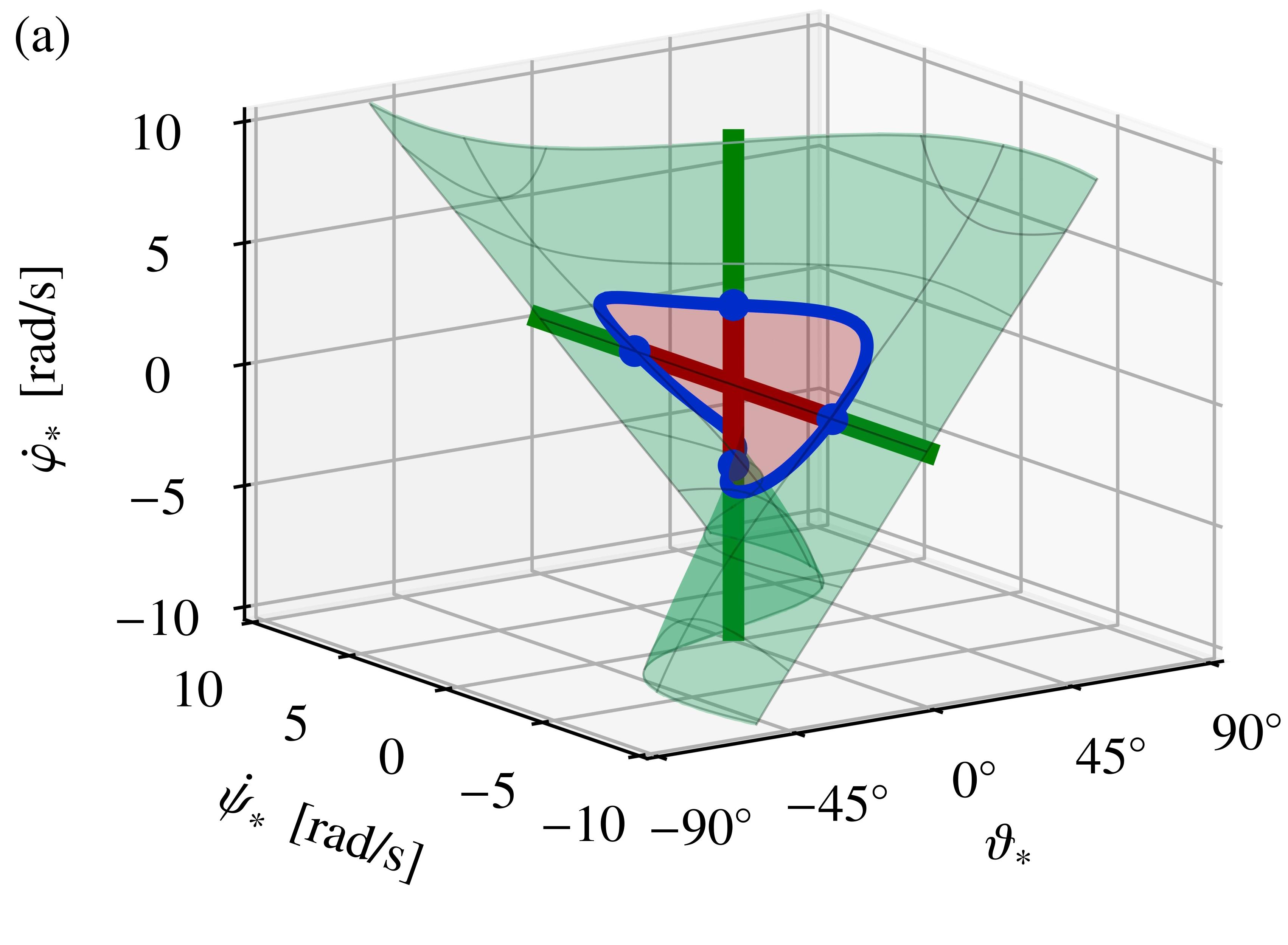
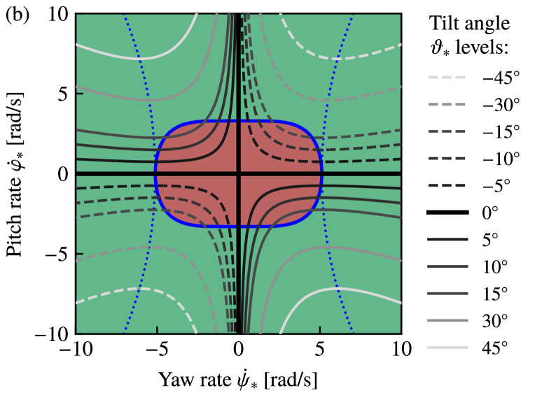
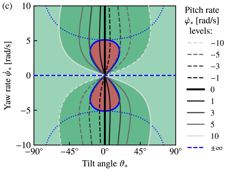
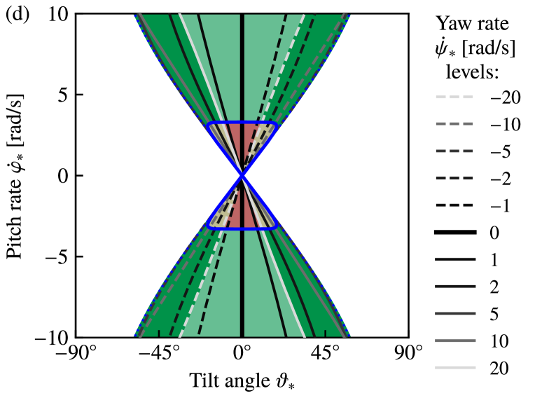
Figure 3: Level sets and stability of steady state motion (13) of the rolling wheel

II-C2 Straight rolling

As discussed above the straight rolling steady state motion (${\dot{\psi}_{*}=0}$) can only occur for zero tilt angle ${\vartheta_{*}=0}$. That is, the steady state (17) simplifies to

$$\omega_{2*}=\dot{\varphi}_{*}\,,\hskip 10.00002pt\varphi_{*}(t)=\dot{\varphi}_{*}t\,,\hskip 10.00002ptx_{\rm G*}(t)=R\dot{\varphi}_{*}t\,,$$ (24)

and all the other states become zero. The state matrix (18) is

$$\mathbf{A}=\begin{bmatrix}0&0&\frac{6}{5}\dot{\varphi}_{*}&\frac{4g}{5R}&0&0&0&0\\ 0&0&0&0&0&0&0&0\\ -2\dot{\varphi}_{*}&0&0&0&0&0&0&0\\ 1&0&0&0&0&0&0&0\\ 0&0&1&0&0&0&0&0\\ 0&1&0&0&0&0&0&0\\ 0&R&0&0&0&0&0&0\\ -R&0&0&0&R\dot{\varphi}_{*}&0&0&0\end{bmatrix}\,,$$ (25)

and the characteristic roots (21) simplify to

$$\lambda_{1,2}=\pm\sqrt{\frac{4g}{5R}-\frac{12}{5}{\dot{\varphi}}_{*}^{2}}\,.$$ (26)

This leads to the critical pitch rate of straight rolling, that is

$${\dot{\varphi}}_{\rm crit}=\sqrt{\frac{g}{3R}}\,,$$ (27)

so the straight rolling steady state is (neutrally) stable if the wheel rolls fast enough ${|\dot{\varphi}_{*}|>\dot{\varphi}_{\rm crit}}$. Otherwise, it is unstable.

We remark that instead of the pitch rate $\dot{\varphi}_{*}$ one may introduce the parameter ${v_{*}=\dot{\varphi}_{*}R}$ which is the steady state velocity of the center of gravity. This way the critical pitch rate (27) can be converted to a critical velocity.

II-C3 Spinning on the spot

The spinning steady state motion (${\dot{\varphi}_{*}=0}$) can also occur for zero tilt angle ${\vartheta_{*}=0}$. Then the steady state becomes

$$\omega_{3*}=\dot{\psi}_{*}\,,\hskip 10.00002pt\psi_{*}=\dot{\psi}_{*}t\,,$$ (28)

and all the other states are zero. The state matrix (18) becomes

$$\mathbf{A}=\begin{bmatrix}0&\frac{6}{5}\dot{\psi}_{*}&0&\frac{4g}{5R}-\frac{1}{5}\dot{\psi}_{*}^{2}&0&0&0&0\\ -\frac{2}{3}\dot{\psi}_{*}&0&0&0&0&0&0&0\\ 0&0&0&0&0&0&0&0\\ 1&0&0&0&0&0&0&0\\ 0&0&1&0&0&0&0&0\\ 0&1&0&-\dot{\psi}_{*}&0&0&0&0\\ R\sin\psi_{*}&R\cos\psi_{*}&0&0&0&0&0&0\\ -R\cos\psi_{*}&R\sin\psi_{*}&0&0&0&0&0&0\end{bmatrix},$$ (29)

while the characteristic roots (21) and the critical yaw rate (22) simplify to

$$\lambda_{1,2} =\pm\sqrt{\frac{4g}{5R}-{\dot{\psi}}_{*}^{2}}\,,$$ (30)

$$\dot{\psi}_{\rm crit} =\sqrt{\frac{4g}{5R}}\,.$$ (31)

That is, the spinning steady state is (neutrally) stable if the wheel spins fast enough ${|{\dot{\psi}}_{*}|>{\dot{\psi}}_{\rm crit}}$. Otherwise, it is unstable.

TABLE I: Numerical parameters for the rolling wheel and unicycle

Quantity	Symbol	Value	Unit
wheel mass	$m$	10	kg
point mass	$m_{0}$	5	kg
wheel radius	$R$	0.3	m
gravitational acceleration	$g$	9.81	m/s2

All results about the steady state motions and their stability are shown in Figure 3. Panel (a) shows the steady state motions (13) as surface in the ($\vartheta_{*}$, $\dot{\psi}_{*}$, $\dot{\varphi}_{*}$) space. Panel (b) shows the level sets of $\vartheta_{*}$ in the ($\dot{\psi}_{*}$, $\dot{\varphi}_{*}$) plane. Similarly, panels (c) and (d) show the level sets of $\dot{\psi}_{*}$ and $\dot{\varphi}_{*}$, respectively. Green ($\blacksquare\!\blacksquare$) and red ($\blacksquare\!\blacksquare$) areas represent stable and unstable steady state solutions, respectively, while the solid blue line (—) is the stability boundary. The dashed blue line (– –) in panel (c) shows where ${\dot{\varphi}_{*}\rightarrow\pm\infty}$. The dotted blue curves ($\cdots$​) in panels (b) and (c) indicate the folding of the surface which are the outer edges of the sand glass shaped colored area in panel (d). In the dark green area ($\blacksquare\!\blacksquare$) in panel (d), two stable steady state states exist with different yaw rates $\dot{\psi}_{*}$, while in the yellow area ($\blacksquare\!\blacksquare$) a stable and an unstable steady state exist. In the white area, no steady state exists regardless of the yaw rate due to the folding of the surface.

III Modeling the unicycle

The unicycle considered here is shown in Figure 4, where the motion is controlled by moving a mass point along the axle of the wheel. In this section, we present the governing equations and analyze the steady states of the open loop system.

III-A Governing equations

The model of the unicycle is built upon the rolling wheel model presented in Section II with the added point mass $m_{0}$ moving along the axle. The mass’ relative position is given by

$$\mathbf{r}_{\rm GA}=\begin{bmatrix}0&r&0\end{bmatrix}_{{\rm F}_{2}}^{\mathsf{T}},$$ (32)

where $r$ represents the position of the point mass along the axle while other two coordinates are restricted to zero by the axle. Between the disc and the point mass, there is an internal pair of forces; the control force acting on the point mass is

$$\mathbf{F}=\begin{bmatrix}0&u&0\end{bmatrix}_{{\rm F}_{2}}^{\mathsf{T}}\,,$$ (33)

while $-\mathbf{F}$ acts on the wheel with opposite sense. The control input $u$ is used for balancing and steering the unicycle.

The equations of motion of the unicycle are derived in Appendix B in a similar way as the model of the rolling wheel; the differences between the two models are highlighted below. The rolling constraints of the wheel are valid in the same form presenting two kinematic constraints and one geometric constraint, see (2) and (3), respectively. Thus, the unicycle is a nonholonomic mechanical system with ${n_{\rm g}=3}$ geometric constraints given in (3) and (32), and ${n_{\rm k}=2}$ kinematic constraints in (2). Accordingly, ${n_{q}=9-n_{\rm g}=6}$ generalized coordinates have to be chosen which describe the system unambiguously; let these be:

$$\begin{split}\big{(}x_{\rm G},\ y_{\rm G},\ \vartheta,\ \psi,\ \varphi,\ r\big{)}\,.\end{split}$$ (34)

Moreover, ${n_{\sigma}=n_{q}-n_{\rm k}=4}$ pseudo velocities have to be chosen; let these be defined by the components of the angular velocity $\bm{\omega}$ of the wheel (see (78) in Appendix B) and the relative speed $\dot{r}$ of the point mass:

$$\begin{split}\omega_{1}&:=\dot{\vartheta}\,,\\ \omega_{2}&:=\dot{\psi}\sin\vartheta+\dot{\varphi}\,,\\ \omega_{3}&:=\dot{\psi}\cos\vartheta\,,\\ \sigma&:=\dot{r}\,.\end{split}$$ (35)

The Appellian approach yields the equations of motion

$$\begin{split}&\begin{cases}\begin{aligned} \dot{\omega}_{1}=&\,\frac{1}{5mR^{2}+4m_{0}r^{2}}\big{(}4\omega_{1}^{2}m_{0}Rr-\omega_{3}^{2}(mR^{2}+4m_{0}r^{2})\tan{\vartheta}\\ &-8\omega_{1}\sigma m_{0}r+2\omega_{2}\omega_{3}R(3mR+2m_{0}r\tan{\vartheta})\\ &-4m_{0}gr\cos{\vartheta}+4mgR\sin{\vartheta}+4Ru\big{)}\,,\\[4.30554pt] \dot{\omega}_{2}=&\,\frac{2}{3mR^{2}+2m_{0}R^{2}+12m_{0}r^{2}}\big{(}-2\omega_{1}\omega_{2}m_{0}Rr\\ &-\omega_{1}\omega_{3}(mR^{2}+m_{0}R^{2}+4m_{0}r^{2})+2\omega_{3}\sigma m_{0}R\big{)}\,,\\[4.30554pt] \dot{\omega}_{3}=&\,\frac{1}{3mR^{2}+2m_{0}R^{2}+12m_{0}r^{2}}\big{(}-2\omega_{1}\omega_{2}R^{2}(3m+2m_{0})\\ &+\omega_{1}\omega_{3}(3mR^{2}\tan{\vartheta}+2m_{0}(R^{2}\tan{\vartheta}+2Rr+6r^{2}\tan{\vartheta}))\\ &-24\omega_{3}\sigma m_{0}r\big{)}\,,\\[4.30554pt] \dot{\vartheta}=&\,\omega_{1}\,,\\[4.30554pt] \dot{\sigma}=&\,\frac{m_{0}}{5mR^{2}+4m_{0}r^{2}}\big{(}\omega_{1}^{2}(5mR^{2}+4m_{0}(R^{2}+r^{2}))r\\ &+\omega_{3}^{2}(5mR^{2}r-4m_{0}Rr^{2}\tan{\vartheta}+4m_{0}r^{3}-mR^{3}\tan{\vartheta})\\ &-8\omega_{1}\sigma R^{2}r+\omega_{2}\omega_{3}R(mR^{2}+4m_{0}(Rr\tan{\vartheta}-r^{2}))\\ &-(mR^{2}+4m_{0}r^{2})g\sin{\vartheta}-4m_{0}gRr\cos{\vartheta}\\ &+(5\tfrac{m}{m_{0}}R^{2}+4R^{2}+4r^{2})u\big{)}\,,\\[4.30554pt] \dot{r}=&\,\sigma\,,\end{aligned}\end{cases}\\ &\begin{cases}\begin{aligned} \dot{\psi}=&\,\omega_{3}\frac{1}{\cos{\vartheta}}\,,\\[4.30554pt] \dot{\varphi}=&\,\omega_{2}-\omega_{3}\tan{\vartheta}\,\,,\\ \dot{x}_{\rm G}=&\,\omega_{1}R\sin{\psi}\cos{\vartheta}+\omega_{2}R\cos{\psi}\,,\\ \dot{y}_{\rm G}=&\,-\omega_{1}R\cos{\psi}\cos{\vartheta}+\omega_{2}R\sin{\psi}\,,\end{aligned}\end{cases}\end{split}$$ (36)

which is a ${n=9-n_{\rm g}-n_{\rm k}/2=5}$ DoF nonholonomic mechanical system. The equations of motion (36) of the unicycle can be divided into essential and hidden dynamics [22]; the essential dynamics consists of the first six equations of (36), while the hidden dynamics are given by the remaining four equations. Observe that the hidden dynamics in the unicycle model (36) is identical to the hidden dynamics of the rolling wheel model (6). Moreover, considering ${m_{0}=0}$ and ${u=0}$ the essential dynamics in (36) simplify to the essential dynamics in (6).

Figure 4: Model of the unicycle for steering

Thanks to the Appellian approach, the dynamical model (36) of the unicycle is naturally formulated as a control affine system ${\dot{\mathbf{x}}=f(\mathbf{x})+g(\mathbf{x})u}$ with the state vector

$$\mathbf{x}=\begin{bmatrix}\omega_{1}&\omega_{2}&\omega_{3}&\vartheta&\sigma&r&\psi&\varphi&x_{\rm G}&y_{\rm G}\end{bmatrix}^{\mathsf{T}}\!.$$ (37)

and control input $u$; cf. (33), so this model is ready for control design.

III-B Steady state motion

Considering ${u\equiv 0}$ (i.e. the point mass freely moves along the axle), the unicycle model (36) possesses the steady state motion with essential dynamics

$$\begin{array}[]{rlrlrl}\omega_{1}(t)&\,\equiv\omega_{1*},&\omega_{2}(t)&\,\equiv\omega_{2*},&\omega_{3}(t)&\,\equiv\omega_{3*},\\ \vartheta(t)&\,\equiv\vartheta_{*},&\sigma(t)&\,\equiv\sigma_{*},&r(t)&\,\equiv r_{*}.\end{array}$$ (40)

Substituting this into the first six equations of (36) yields

$$\begin{split}&\omega_{2*}\omega_{3*}\big{(}{6mR^{2}}+{4m_{0}Rr_{*}\tan{\vartheta_{*}}}\big{)}-\omega_{3*}^{2}\big{(}{mR^{2}}+{4m_{0}r_{*}^{2}}\big{)}\tan{\vartheta_{*}}\\ &\quad-{4m_{0}gr_{*}\cos{\vartheta_{*}}}+{4mgR\sin{\vartheta_{*}}}=0\,,\\[4.30554pt] &\omega_{2*}\omega_{3*}\big{(}{mm_{0}R^{3}}-{4m_{0}^{2}Rr_{*}^{2}}+{4m_{0}^{2}R^{2}r_{*}\tan{\vartheta_{*}}}\big{)}\\ &\quad+\omega_{3*}^{2}\big{(}{5mm_{0}R^{2}r_{*}}+{4m_{0}^{2}r_{*}^{3}-({mm_{0}R^{3}}+{4m_{0}^{2}Rr_{*}^{2})\tan{\vartheta_{*}}}}\big{)}\\ &\quad-({4m_{0}^{2}gr_{*}^{2}}+{mm_{0}gR^{2})\sin{\vartheta_{*}}}-{4m_{0}^{2}gRr_{*}\cos{\vartheta_{*}}}=0\,.\end{split}$$ (41)

The hidden motion of the unicycle is the same as the hidden motion of the wheel which is described by (10) and (11).

Using (35), the relations (41) can be reformulated using the generalized velocities $\dot{\psi}_{*}$, $\dot{\vartheta}_{*}$, $\dot{\varphi}_{*}$, and $\dot{r}_{*}$:

$$\begin{split}&{}{5mR^{2}\dot{\psi}_{*}^{2}\sin{\vartheta_{*}}\cos{\vartheta_{*}}}+{4m_{0}R\dot{\psi}_{*}^{2}r_{*}\sin^{2}{\vartheta_{*}}}\\ &\quad-{4m_{0}\dot{\psi}_{*}^{2}r_{*}^{2}\sin{\vartheta_{*}}\cos{\vartheta_{*}}}+{6mR^{2}\dot{\psi}_{*}\dot{\varphi}_{*}\cos{\vartheta_{*}}}\\ &\quad+{4m_{0}R\dot{\psi}_{*}\dot{\varphi}_{*}r_{*}\sin{\vartheta_{*}}}-{4m_{0}gr_{*}\cos{\vartheta_{*}}}\\ &\quad+{4mgR\sin{\vartheta_{*}}}=0\,,\\[4.30554pt] &{}{mR^{3}\dot{\psi}_{*}\dot{\varphi}_{*}\cos{\vartheta_{*}}}+{4m_{0}R^{2}\dot{\psi}_{*}\dot{\varphi}_{*}r_{*}\sin{\vartheta_{*}}}\\ &\quad-{4m_{0}R\dot{\psi}_{*}\dot{\varphi}_{*}r_{*}^{2}\cos{\vartheta_{*}}}+{5mR^{2}\dot{\psi}_{*}^{2}r_{*}\cos^{2}{\vartheta_{*}}}\\ &\quad+{4m_{0}R^{2}\dot{\psi}_{*}^{2}r_{*}\sin^{2}{\vartheta_{*}}}-{8m_{0}R\dot{\psi}_{*}^{2}r_{*}^{2}\sin{\vartheta_{*}}\cos{\vartheta_{*}}}\\ &\quad+{4m_{0}\dot{\psi}_{*}^{2}r_{*}^{3}\cos^{2}{\vartheta_{*}}}-{mgR^{2}\sin{\vartheta_{*}}}-{4m_{0}gRr_{*}\cos{\vartheta_{*}}}\\ &\quad-{4m_{0}gr_{*}^{2}\sin{\vartheta_{*}}}=0\,.\end{split}$$ (42)

Similarly to the rolling wheel, one may express the steady state pitch rate $\dot{\varphi}_{*}$ and point mass position $r_{*}$ as a function of the the tilt angle $\vartheta_{*}$ and the yaw rate $\dot{\psi}_{*}$:

$$\begin{split}\dot{\varphi}_{*}&=\frac{1}{\dot{\psi}_{*}R(6mR\cos{\vartheta_{*}+4m_{0}r_{*}\sin{\vartheta_{*}})}}\big{(}-4mgR\sin{\vartheta_{*}}\\ &\quad+\dot{\psi}_{*}^{2}(4m_{0}r_{*}^{2}-5mR^{2})\sin{\vartheta_{*}}\cos{\vartheta_{*}}\\ &\quad-4\dot{\psi}_{*}^{2}m_{0}Rr_{*}\sin^{2}{\vartheta_{*}}+4m_{0}gr_{*}\cos{\vartheta_{*}}\big{)}\,,\\[4.30554pt] r_{*}&=\frac{mR(\dot{\psi}_{*}^{2}R\cos{\vartheta_{*}}+2g)\sin{\vartheta_{*}}\cos{\vartheta_{*}}}{6\dot{\psi}_{*}^{2}mR\cos^{3}{\vartheta_{*}}-4m_{0}g}\,,\end{split}$$ (43)

if

$$\begin{split}\dot{\psi}_{*}&\neq 0\,,\quad\dot{\psi}_{*}\neq\pm\sqrt{\dfrac{2m_{0}g}{3mR\cos^{3}{\vartheta_{*}}}},\end{split}$$ (44)

holds. Note that the steady state point mass position $r_{*}$ must be substituted into the expression of the steady state pitch rate $\dot{\varphi}_{*}$ in (43). For the non-generic cases when (44) does not hold, the steady state motions are explained below.

When the yaw rate is zero ${\dot{\psi}_{*}=0}$, straight rolling occurs and (42) simplify to

$$\begin{split}&{4mR\sin{\vartheta_{*}}}-{4m_{0}r_{*}\cos{\vartheta_{*}}}=0\,,\\ &\big{(}{mR^{2}+{4m_{0}r_{*}^{2}}\big{)}\sin{\vartheta_{*}}}+{4m_{0}Rr_{*}\cos{\vartheta_{*}}}=0\,.\end{split}$$ (45)

These are only satisfied for zero tilt angle ${\vartheta_{*}=0}$, which also implies the centered position of the point mass ${r_{*}=0}$. Since the pitch rate $\dot{\varphi}_{*}$ does not appear in (45), it can be arbitrary similarly to straight rolling of the wheel.

In case of ${\dot{\psi}_{*}=\pm\sqrt{{2m_{0}g}/({3mR\cos^{3}{\vartheta_{*}}})}}$, (42) still results in zero tilt angle ${\vartheta_{*}=0}$ and the relations simplify to

$$\begin{split}\dot{\psi}_{*1,2}&=\pm\sqrt{\frac{{2}{m_{0}}{g}}{3{m}{R}}}\,,\quad\dot{\varphi}_{*1,2}=\pm\sqrt{\dfrac{{2}{m_{0}}{g}}{3mR^{3}}}r_{*}\,,\end{split}$$ (46)

which describe a turning-rolling steady state motion with a non-tilted wheel. This is a new behavior of the unicycle which does not exist for rolling wheel, since the rolling disc must be tilted in order to have a turning-rolling steady state motion, cf. (13). Note that, this steady state can only occur for the specific yaw rates ${\dot{\psi}_{*1,2}}$ depending only on physical parameters, while the corresponding pitch rates ${\dot{\varphi}_{*1,2}}$ also depend only on the point mass position $r_{*}$. The non-tilted turning steady state becomes a spinning steady state (${\dot{\varphi}_{*1,2}}=0$) if the point mass is at the center ${r_{*}=0}$.

The other spinning steady state can be obtained by substituting zero pitch rate ${\dot{\varphi}_{*}=0}$ into (42), which yields

$$\begin{split}&\dot{\psi}_{*}^{2}\big{(}(5mR^{2}-4m_{0}r_{*}^{2})\sin{\vartheta_{*}}\cos{\vartheta_{*}}+{4m_{0}Rr_{*}\sin^{2}{\vartheta_{*}}}\big{)}\\ &\quad+{4mgR\sin{\vartheta_{*}}}-{4m_{0}gr_{*}\cos{\vartheta_{*}}}=0\,,\\[4.30554pt] &\dot{\psi}_{*}^{2}\big{(}({5mr_{*}R^{2}}-{4m_{0}R^{2}r_{*}+{4m_{0}r_{*}^{3}})\cos^{2}{\vartheta_{*}}}+{4m_{0}R^{2}r_{*}}\\ &\quad-{8m_{0}Rr_{*}^{2}\sin{\vartheta_{*}}\cos{\vartheta_{*}}}\big{)}-{(mgR^{2}+{4m_{0}gr_{*}^{2}})\sin{\vartheta_{*}}}\\ &\quad-{4m_{0}gRr_{*}\cos{\vartheta_{*}}}=0\,.\end{split}$$ (47)

Similar to the spinning wheel, such steady state motion exists for zero tilt angle (${\vartheta_{*}=0}$) when the point mass is at the center ${r_{*}=0}$. However, in case of the unicycle, spinning type steady state motion also exists with non-zero tilt angle (${\vartheta_{*}\neq 0}$) when

$$\begin{split}\dot{\psi}_{*}&=\pm\sqrt{\frac{4m_{0}gr_{*}\cos{\vartheta_{*}}-4mgR\sin{\vartheta_{*}}}{(5mR^{2}-4m_{0}r_{*}^{2})\sin{\vartheta_{*}}\cos{\vartheta_{*}}+4m_{0}Rr_{*}\sin^{2}{\vartheta_{*}}}}\,,\\[4.30554pt] r_{*}&=\frac{R\tan{\vartheta_{*}}}{2m_{0}}\Big{(}m\cos^{2}{\vartheta_{*}}+m_{0}\\ &\quad+\sqrt{m^{2}\cos^{4}{\vartheta_{*}}+3mm_{0}\cos^{2}{\vartheta_{*}}+m_{0}^{2}}\Big{)}\,.\end{split}$$ (48)

We refer to this steady state as tilted spinning, which is also a new behavior of the unicycle compared to the rolling wheel. According to (48), the point mass is always above the wheel center since ${{\rm sgn}\,r_{*}={\rm sgn}\,\vartheta_{*}}$ or ${r_{*}\,\vartheta_{*}>0}$; (cf. Figure 4). Investigating special cases like ${\vartheta_{*}=0}$ or ${r_{*}=0}$ leads to steady states already discussed above.

One limiting factor of our unicycle model is that the point mass may slide below the ground which is physically not feasible. To exclude these cases, one can calculate the $z$ coordinate of the position vector $\mathbf{r}_{\rm A}=\mathbf{r}_{\rm G}+\mathbf{r}_{\rm GA}$ of the point mass in frame ${\rm F_{0}}$ and require it to be positive. This yields the condition

$$R\cos{\vartheta_{*}}+r_{*}\sin{\vartheta_{*}}>0\,.$$ (49)

All steady state motions of the unicycle are summarized in Figure 5 in the plane of the steady state tilt angle $\vartheta_{*}$ and the yaw rate ${\dot{\psi}_{*}}$.

The corresponding pitch rate $\dot{\varphi}_{*}$ and the point mass position $r_{*}$ can be expressed by (43). The non-generic steady states are the straight rolling and the non-tilted turning. The straight rolling, i.e. ${\vartheta_{*}=0}$ and ${\dot{\psi}_{*}=0}$, is marked by a black square $\blacksquare$; in this case the steady state pitch rate $\dot{\varphi}_{*}$ may be arbitrary and the point mass is at wheel center ${r_{*}=0}$. The non-tilted turning, i.e. ${\vartheta_{*}=0}$ and ${\dot{\psi}_{*}=\dot{\psi}_{*1,2}}$, is marked by black dots $\CIRCLE$; in this case the pitch rate $\dot{\varphi}_{*}$ and the point mass position $r_{*}$ linked as in (46).

The regular (non-tilted) spinning steady state motions, i.e. ${\vartheta_{*}=0}$ and ${\dot{\varphi}_{*}=0}$, are shown by the solid black line (—); in this case the yaw rate $\dot{\psi}_{*}$ may be arbitrary and the point mass is at the wheel center ${r_{*}=0}$. The tilted spinning steady states, i.e. ${\dot{\varphi}_{*}=0}$ and ${\vartheta_{*}\neq 0}$, are shown by dashed black lines (– –); the corresponding yaw rate $\dot{\psi}_{*}$ and point mass position $r_{*}$ are expressed by (48).

The general turning-rolling steady states are divided into separate areas. The light blue $\blacksquare\!\blacksquare$ and light purple $\blacksquare\!\blacksquare$ areas show the physically feasible steady states when the point mass is placed below ${0<z_{\rm A}<z_{\rm G}}$ or above ${z_{\rm A}>z_{\rm G}}$ the wheel center point $\rm G$, respectively. The white area $\bm{\sqsubset}\!\bm{\sqsupset}$ represents the physically unfeasible steady states when the point mass is at or below the ground level, that is, ${z_{\rm A}\leq 0}$.

Note that, Figure 5 was constructed using the numerical parameters in Table I; using different parameters, like different mass ratios ${m_{0}/m}$, the main structure of the steady states remain qualitatively similar but the shape and size of the parameter regions related to the non-feasible steady states may be different.

The steady states have been categorized with considering zero input force (${u\equiv 0}$). Assuming a nonzero constant input (${u\equiv u_{*}}$) may result in further steady states. For example, a straight rolling case may occur with tilted wheel when the mass is held ‘above’ the wheel center. Studying such steady states are out of the scope of the present study.

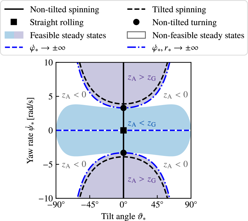
Figure 5: Summary of the steady state motions of the unicycle

III-C Stability of steady states

Linear stability analysis is performed to determine the stability of the previously discussed steady state motions of the unicycle. Linearizing (36) around a steady state $\mathbf{x}_{*}$ leads to the form ${\dot{\tilde{\mathbf{x}}}=\mathbf{A}\tilde{\mathbf{x}}}$ where ${\tilde{\mathbf{x}}=\mathbf{x}-\mathbf{x}_{*}}$ denotes the perturbed states and state matrix ${\mathbf{A}=f^{\prime}(\mathbf{x}_{*})}$ can be written as

$$\mathbf{A}=\begin{bmatrix}0&A_{12}&A_{13}&A_{14}&0&A_{16}&0&0&0&0\\ A_{21}&0&0&0&A_{25}&0&0&0&0&0\\ A_{31}&0&0&0&A_{35}&0&0&0&0&0\\ 1&0&0&0&0&0&0&0&0&0\\ 0&A_{52}&A_{53}&A_{54}&0&A_{56}&0&0&0&0\\ 0&0&0&0&1&0&0&0&0&0\\ 0&0&A_{73}&A_{74}&0&0&0&0&0&0\\ 0&1&A_{83}&A_{84}&0&0&0&0&0&0\\ A_{91}&A_{92}&0&0&0&0&A_{97}&0&0&0\\ A_{101}&A_{102}&0&0&0&0&A_{107}&0&0&0\end{bmatrix},$$ (50)

whose elements are given in Appendix C. Note that the steady state tilt angle $\vartheta_{*}$, yaw rate $\dot{\psi}_{*}$, pitch rate $\dot{\varphi}_{*}$ and point mass position $r_{*}$ in the elements of $\mathbf{A}$ are not independent of each other, they must satisfy (42). Therefore, each of the different steady state motions (turning-rolling, straight rolling, non-tilted turning) must be analyzed separately. In this paper we focus on the straight rolling and turning-rolling motions while the non-tilted turning is left for future research. Also note that, the spinning steady state is a special case of the more general turning-rolling steady state; since it has minor practical relevance its further analysis is omitted.

The characteristic equation ${\det(\lambda\mathbf{I}-\mathbf{A})=0}$ takes the form

$$\begin{split}&\big{(}\lambda^{4}-\lambda^{2}(A_{12}A_{21}+A_{13}A_{31}+A_{14}+A_{25}A_{52}+A_{35}A_{53}+A_{56})\\ &+A_{12}A_{21}A_{35}A_{53}+A_{12}A_{21}A_{56}-A_{12}A_{31}A_{25}A_{53}-A_{12}A_{25}A_{54}\\ &+A_{13}A_{31}A_{25}A_{52}+A_{13}A_{31}A_{56}-A_{13}A_{21}A_{35}A_{52}-A_{13}A_{35}A_{54}\\ &+A_{14}A_{25}A_{52}+A_{14}A_{35}A_{53}+A_{14}A_{56}\\ &-A_{16}A_{21}A_{52}-A_{16}A_{31}A_{53}-A_{16}A_{54}\big{)}\lambda^{6}=0\,.\end{split}$$ (51)

This is independent of the matrix elements $A_{73}$, $A_{74}$, $A_{83}$, $A_{84}$, $A_{91}$, $A_{92}$, $A_{97}$, $A_{101}$, $A_{102}$ and $A_{107}$, which corresponds to the hidden states $\psi$, $\varphi$, $x_{\rm G}$ and $y_{\rm G}$.

III-C1 Turning-rolling steady state

During the stability analysis, the characteristic roots of (LABEL:eq:chp_general_unicycle) are analyzed, where the steady state pitch rate $\dot{\varphi}_{*}$ and point mass position $r_{*}$ must be substituted according to (43). Due to the highly complicated expressions, numerical evaluation is used to obtain the characteristic roots and determine the stability of the turning-rolling steady states. The results are shown in Figure 6 for several mass ratios with ${m_{0}=0,1,2,5,10,15,20,30}$ kg, while the other physical parameters are presented in Table I. The same coloring scheme is used as in Fig. 3.

III-C2 Straight rolling

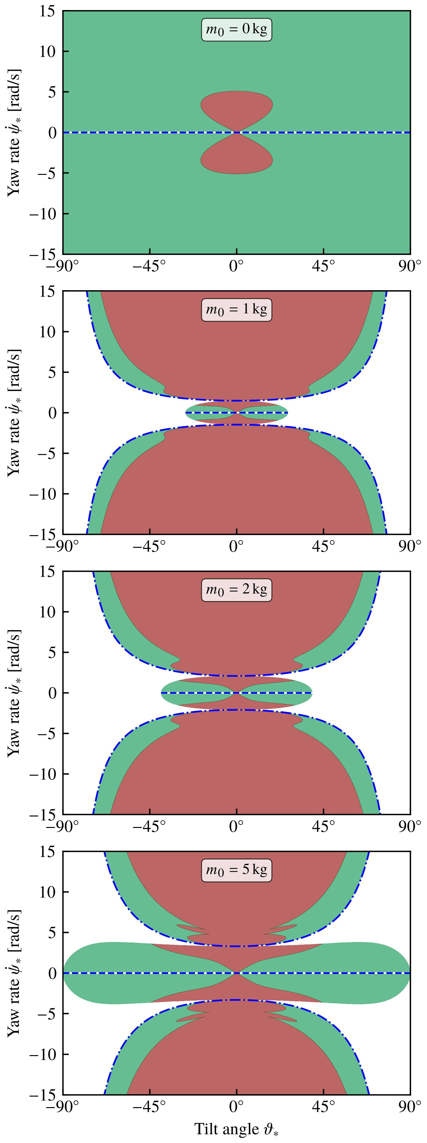
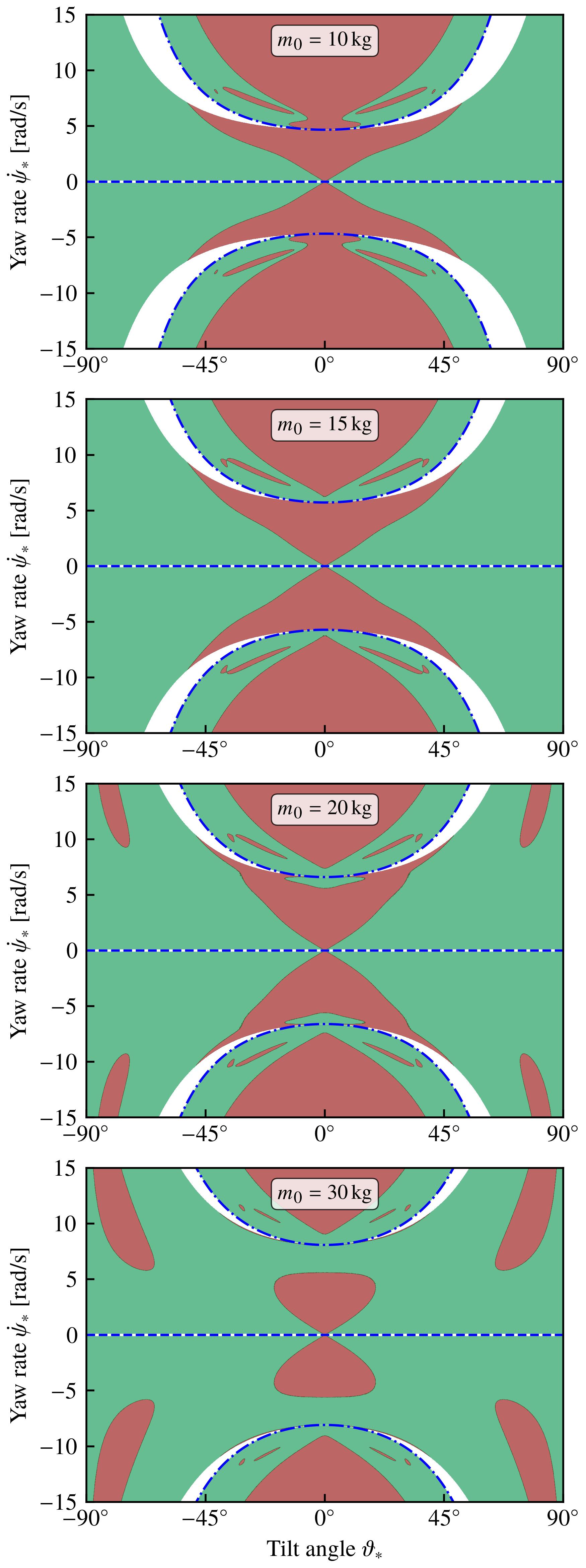
Figure 6: Stability of steady state motions of the unicycle for different $m_{0}$ values

The corresponding steady state can be given as (24) and all the other states become zero, considering that the initial values $x_{\rm 0}$, $y_{\rm 0}$ and $\dot{\psi}_{0}$ are zeros. In this case, the state matrix (50) simplifies to

$$\mathbf{A}=\begin{bmatrix}0&0&\frac{6}{5}\dot{\varphi}_{*}&\frac{4g}{5R}&0&-\frac{4m_{0}g}{5mR^{2}}&0&0&0&0\\ 0&0&0&0&0&0&0&0&0&0\\ -2\dot{\varphi}_{*}&0&0&0&0&0&0&0&0&0\\ 1&0&0&0&0&0&0&0&0&0\\ 0&0&\frac{R}{5}\dot{\varphi}_{*}&-\frac{g}{5}&0&-\frac{4m_{0}g}{5mR}&0&0&0&0\\ 0&0&0&0&1&0&0&0&0&0\\ 0&0&1&0&0&0&0&0&0&0\\ 0&1&0&0&0&0&0&0&0&0\\ 0&R&0&0&0&0&0&0&0&0\\ -R&0&0&0&0&0&R\dot{\varphi}_{*}&0&0&0\end{bmatrix}.$$ (52)

When comparing this with (25) obtained for the rolling wheel, there are two extra rows and columns, 5 and 6, related to the new states $r$ and $\sigma$.

The characteristic polynomial (LABEL:eq:chp_general_unicycle) reduces to

$$\begin{split}\big{(}a\lambda^{4}+b\lambda^{2}+c\big{)}\lambda^{6}=0\,,\end{split}$$ (53)

where

$$\begin{split}a&={5mR^{2}},\,\\ b&={12\dot{\varphi}_{*}^{2}mR^{2}+4(m_{0}-m)gR},\,\\ c&=4m_{0}g({2\dot{\varphi}_{*}^{2}R-g}).\end{split}$$ (54)

The system is stable if the coefficients $a,b$ and $c$ have the same sign. While $a>0$ always holds, $b>0$ and $c>0$ lead to

$$|\dot{\varphi}_{*}|>\sqrt{\frac{(m-m_{0})g}{3mR}}\quad\text{ and }\quad|\dot{\varphi}_{*}|>\sqrt{\frac{g}{2R}}\,,$$ (55)

respectively. The second condition is always stronger, so the critical pitch rate of the unicycle is

$$\dot{\varphi}_{\rm crit}=\sqrt{\frac{g}{2R}}\,.$$ (56)

That is, the straight rolling of the uncontrolled unicycle is (neutrally) stable if ${|\dot{\varphi}_{*}|>\dot{\varphi}_{\rm crit}}$; it is unstable if ${|\dot{\varphi}_{*}|<\dot{\varphi}_{\rm crit}}$.

Note that, the critical pitch rate (56) is independent of the masses $m$ and $m_{0}$. Also, it is larger than the critical pitch rate of the rolling disc (27). The dependency of the characteristic roots on the steady state pitch rate $\dot{\varphi}_{*}$ are summarized in Figure 7 for both the rolling disc (${m_{0}=0}$) and the unicycle (${m_{0}>0}$). Observe that while in case of the rolling wheel the characteristic roots $\lambda_{1,2}$ (thick gray curves) determine the criticality, in case of the unicycle (even for small values of $m_{0}$!) the criticality is determined by the characteristic roots $\lambda_{3,4}$ (orange curves) rather than by the characteristic roots $\lambda_{1,2}$ (blue curves). This resolves the seemingly contradictory issue that the critical pitch rate “jumps” form (27) to (56) when $m_{0}$ becomes positive.

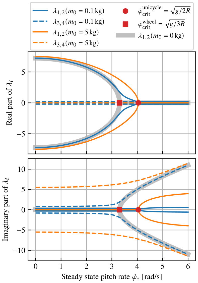
Figure 7: Characteristic roots as a funtion the steady state pitch rate $\dot{\varphi}_{*}$ comparing the cases of rolling wheel and unicycle

III-C3 Spinning on the spot

The stability analysis of this steady state is covered by the analysis of the turning-rolling motion. Since the motion has minor practical relevance for unicycles further discussions are omitted here.

IV Steering control of the unicycle

The straight rolling steady state (24) is used as the basis for designing the steering controller of the unicycle. For simplicity, it is assumed that the unicycle has an initial pitch rate ${\dot{\varphi}_{0}=\dot{\varphi}_{*}}$ and initially it travels along the $x_{0}$ axis. Above we showed that the straight rolling steady state might be unstable or neutrally stable without control. Here we demonstrate that this motion can be made asymptotically stable with appropriate feedback control.

The linear state space model of the unicycle assumes the form where ${\tilde{\mathbf{x}}=\mathbf{x}-\mathbf{x}_{*}}$. The state matrix ${\mathbf{A}=f^{\prime}(\mathbf{x}_{*})}$ is given in (52) and it depends on the steady state pitch rate $\dot{\varphi}_{*}$. The input matrix ${\mathbf{B}=g^{\prime}(\mathbf{x}_{*})}$ is given by

$$\begin{split}\mathbf{B}&=\begin{bmatrix}\frac{4}{5mR}\ \ 0\ \ 0\ \ 0\ \ \frac{5m+4m_{0}}{5mm_{0}}\ \ 0\ \ 0\ \ 0\ \ 0\ \ 0\end{bmatrix}^{\mathsf{T}}.\end{split}$$ (57)

IV-A Controllability

The controllability matrix of the unicycle can be obtained as

$$\begin{split}\mathbf{M}_{\rm c}=\begin{bmatrix}\mathbf{B}\ \ \mathbf{A}\mathbf{B}\ \ \mathbf{A}^{\!2}\mathbf{B}\ \ \dots\ \ \mathbf{A}^{\!9}\mathbf{B}\end{bmatrix}.\end{split}$$ (58)

Substituting (52) and (57) we obtain

$$\mathbf{M}_{\rm c}=\begin{bmatrix}M_{11}&M_{12}&M_{13}&0&0&M_{16}&0&0&M_{19}&0\\ 0&0&0&0&0&0&0&0&0&0\\ 0&0&0&cM_{44}&cM_{45}&0&cM_{47}&cM_{48}&0&cM_{410}\\ 0&0&0&M_{44}&M_{45}&0&M_{47}&M_{48}&0&M_{410}\\ M_{51}&M_{52}&M_{53}&0&0&M_{56}&0&0&M_{59}&0\\ 0&0&0&M_{64}&M_{65}&0&M_{67}&M_{68}&0&M_{610}\\ 0&M_{72}&M_{73}&0&0&M_{76}&0&0&M_{79}&0\\ 0&0&0&0&0&0&0&0&0&0\\ 0&0&0&0&0&0&0&0&0&0\\ 0&0&0&M_{104}&M_{105}&0&M_{107}&M_{108}&0&M_{1010}\!\end{bmatrix}\!,$$ (59)

with ${c=-2\dot{\varphi}_{*}}$. Notice that rows 2, 8 and 9 are full of zeros while rows 3 and 4 are linearly dependent. Thus, ${\mathrm{rank}\,\mathbf{M}_{\rm c}=6}$ and the controllability matrix is not full row rank. That is, at the linear level, the unicycle is not fully controllable with the single input $u$.

When spelling out the 3^rd and 4^th equations in the linear system ${\dot{\tilde{\mathbf{x}}}=\mathbf{A}\tilde{\mathbf{x}}+\mathbf{B}u}$ one obtains

$$\begin{split}\dot{\omega}_{3}&=-2\dot{\varphi}_{*}\omega_{1}\,,\\ \dot{\vartheta}&=\omega_{1}\,\end{split}$$ (60)

which lead to

$$\omega_{3}=-2\dot{\varphi}_{*}\vartheta\,.$$ (61)

This means that the yaw rate $\dot{\psi}$ is linearly proportional to the tilt angle $\vartheta$, since $\omega_{3}\approx\dot{\psi}$ for small tilt angles; cf. (35). That is, to steer the unicycle it is necessary to tilt it accordingly.

Note that one may steer the unicycle with a specific yaw rate $\dot{\psi}_{*}$ in (46) even with zero tilt angle, but model must be linearized around the non-tilted turning steady state of the unicycle. This is left for future research.

IV-B Maneuvering

In this study, two maneuvers are considered for the steering control of the unicycle: a lane change and a $90^{\circ}$ right turn while assuming that the unicycle initially travels along the $x_{0}$ axis. Considering the steady state velocity ${v_{\mathrm{G}*}=R\dot{\varphi}_{*}}$ of the center of gravity leads to the critical speed ${v_{\mathrm{G,crit}}=\sqrt{Rg/2}}$ for the critical pitch rate $\dot{\varphi}_{\mathrm{crit}}$ in (56). For the parameters in Table I, we obtain ${v_{\mathrm{G,crit}}\approx 1.21}$ m/s². Thus, both of the maneuvers are investigated for two speeds: ${v_{\mathrm{G}1}=1\,\mathrm{m/s}}$ which is below the critical speed, and ${v_{\mathrm{G}2}=5\,\mathrm{m/s}}$ which is above the critical speed.

When designing the controllers to execute these maneuvers, the non-reachable states $\omega_{2}$, $\omega_{3}$, $\varphi$, $x_{\rm G}$ are omitted; cf. (37) and (59). Then, according to the state matrix (52) and input matrix (57) the reduced system becomes

$$\begin{split}\dot{\omega}_{1}&=\bigg{(}\frac{4g}{5R}-\frac{12}{5}\dot{\varphi}_{*}^{2}\bigg{)}\vartheta-\frac{4m_{0}g}{5mR^{2}}r+\frac{4}{5mR}u\,,\\ \dot{\vartheta}&=\omega_{1}\,,\\ \dot{\sigma}&=-\bigg{(}\frac{g}{5}+\frac{2R}{5}\dot{\varphi}_{*}^{2}\bigg{)}\vartheta-\frac{4m_{0}g}{5mR}r+\frac{5m+4m_{0}}{5mm_{0}}u\,,\\ \dot{r}&=\sigma\,,\\ \dot{\psi}&=-2\dot{\varphi}_{*}\vartheta\,,\\ \dot{y}_{\rm G}&=-R\omega_{1}+R\dot{\varphi}_{*}\psi\,,\end{split}$$ (62)

where the tildes above the states (representing perturbations) are omitted since the equilibrium values are zeros for all these states. We formally define the states in this reduced system as outputs of the full linear system ${\dot{\tilde{\mathbf{x}}}=\mathbf{A}\tilde{\mathbf{x}}+\mathbf{B}u}$ when designing the controllers for the lane change and turning maneuvers.

IV-B1 Lane change

For the lane change maneuver the state $y_{\rm G}$ can be utilized to plan the motion since the unicycle should move parallel to the $x_{0}$ axis at the beginning and at the end of the maneuver. According to this, we consider the input

$$\mathbf{y}=\mathbf{C}\mathbf{x}:=\begin{bmatrix}\omega_{1}&\vartheta&\sigma&r&\psi&y_{\rm G}\end{bmatrix}^{\mathsf{T}},$$ (63)

(cf. (62)) with

$$\mathbf{C}=\begin{bmatrix}1&0&0&0&0&0&0&0&0&0\\ 0&0&0&1&0&0&0&0&0&0\\ 0&0&0&0&1&0&0&0&0&0\\ 0&0&0&0&0&1&0&0&0&0\\ 0&0&0&0&0&0&1&0&0&0\\ 0&0&0&0&0&0&0&0&0&1\end{bmatrix}.$$ (64)

The output controllability matrix can be constructed as

$$\begin{split}\mathbf{M}_{\rm oc}=\begin{bmatrix}\mathbf{C}\mathbf{B}\ \ \mathbf{C}\mathbf{A}\mathbf{B}\ \ \mathbf{C}\mathbf{A}^{\!2}\mathbf{B}\ \ \dots\ \ \mathbf{C}\mathbf{A}^{\!9}\mathbf{B}\end{bmatrix},\end{split}$$ (65)

which has a maximal row rank ${\mathrm{rank}\,\mathbf{M}_{\rm oc}=6}$. That is, the unicycle is output controllable.

To control the unicycle, we apply the linear output feedback law

$$u:=-\mathbf{K}(\mathbf{y}-\mathbf{y}_{\rm des})\,,$$ (66)

with control gains ${\mathbf{K}=[D_{\vartheta}\ P_{\vartheta}\ D_{r}\ P_{r}\ P_{\psi}\ P_{y}]}$ and

$$\begin{array}[]{rcccccccccccl}\mathbf{y}_{\rm des}=[&0&&0&&0&&0&&0&&y_{\rm des}(t)&]^{\mathsf{T}}\,,\end{array}$$ (67)

where $y_{\rm des}(t)$ encodes the desired trajectory in terms of $y_{\rm G}$. Here we consider

$$\begin{split}y_{\rm des}(t)&=\begin{cases}\begin{array}[]{lrl}0,&0\leq&~{}t<2,\\ L\big{(}\cos\big{(}\tfrac{\pi}{5}(t-2)\big{)}-1\big{)},&2\leq&~{}t<7,\\ -L,&7\leq&~{}t<10;\\ \end{array}\end{cases}\end{split}$$ (68)

and we use ${L=2.5\,{\rm m}}$ for speed ${v_{\mathrm{G}1}=1\,\mathrm{m/s}}$ and ${L=10\,{\rm m}}$ for speed ${v_{\mathrm{G}2}=2\,\mathrm{m/s}}$. The desired trajectories are depicted as a black dashed-dotted curves in the ${(x_{0},y_{0})}$-plane in the bottom left panel in Fig. 8. For simplicity, we consider the desired yaw angle ${{\dot{\psi}_{\rm des}}(t)\equiv 0}$ in (67). More sophisticated reference trajectories might be constructed utilizing (42).

Note that there are two derivative gains and four proportional gains in this control law, which follows from the Appellian description of the unicycle. The characteristic equation of the closed-loop system is

$$\det\big{(}\lambda\mathbf{I}-(\mathbf{A-BKC})\big{)}=0\,.$$ (69)

By selecting the control gains in $\mathbf{K}$ appropriately one may place the non-zero characteristic roots to the left half complex plane and guarantee stability for the closed-loop system. In particular, using the control gains in Table II results in ${\lambda_{k}=-8}$ s^-1, ${k=1,\dots,6}$.

TABLE II: Control gains for the lane change maneuver

Below critical speed
${v_{\mathrm{G}1}<v_{\mathrm{G,crit}}}$
	$D_{\vartheta}$	$\mathbf{-2042.70}$	Ns
	$P_{\vartheta}$	$\mathbf{-7637.29}$	N
	$D_{r}$	$2116.86$	Ns/m
	$P_{r}$	$11942.04$	N/m
	$P_{\psi}$	$3382.02$	N
	$P_{y}$	$4509.36$	N/m

Above critical speed
${v_{\mathrm{G}2}>v_{\mathrm{G,crit}}}$
	$D_{\vartheta}$	$\mathbf{75.51}$	Ns
	$P_{\vartheta}$	$\mathbf{777.28}$	N
	$D_{r}$	$99.52$	Ns/m
	$P_{r}$	$405.60$	N/m
	$P_{\psi}$	$676.4$	N
	$P_{y}$	$180.37$	N/m

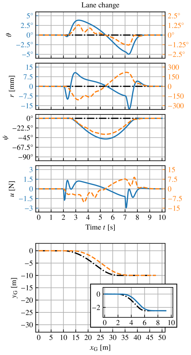
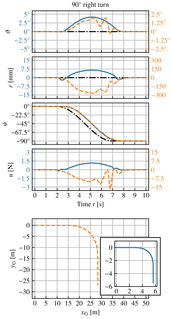
Figure 8: Maneuvers: lane change (left column) and 90^∘ right turn (right column) for subcritical speed (solid blue) and supercritical speed (dashed orange)

The performance of the closed loop system is demonstrated by numerical simulations in the left column in Fig. 8 The simulations were carried out using the full nonlinear equations of motion (36) applying the control law (66) with reference trajectory (68) and control gains in Table II. The time evolution of tilt angle $\vartheta$, point mass position $r$, yaw angle $\psi$, and the control input $u$ are depicted in the top four panels, while the bottom panel shows the movement of the wheel center $\rm G$ above the ${(x_{0},y_{0})}$-plane. The desired lane change maneuver is followed by the unicycle, and the controller successfully stabilizes the desired motion for both speeds. The gains $P_{\vartheta}$ and $D_{\vartheta}$ are highlighted in Table II as they have opposite signs above and below the critical speed. Below the critical speed (${v_{\mathrm{G}1}<v_{\mathrm{G,crit}}}$), the open loop dynamics is unstable, here the $P_{\vartheta}$ and $D_{\vartheta}$ gains correspond to positive stiffness and damping in the mechanical sense. In contrast, above the critical speed (${v_{\mathrm{G}2}>v_{\mathrm{G,crit}}}$) the open loop dynamics is (neutrally) stable and the $P_{\vartheta}$ and $D_{\vartheta}$ gains correspond to negative stiffness and damping. This illustrates that executing a lane change maneuver above the critical speed takes more effort, since the straight-rolling motion of the open-loop systems is more stable. This can also be observed when comparing the required control input for the different speeds. Still the required control input remains small (${|u|<10}$ N) for both speeds.

IV-B2 90^∘ Turn

For the 90^∘ right turn maneuver, the unicycle moves parallel to the $y_{0}$ axis and the state $y_{\rm G}$ becomes unreachable by the control input. Thus, the state $y_{\rm G}$ may not be used to plan motion in this case. Instead we use the yaw angle $\psi$ to construct the reference trajectory. Considering this, the output vector

$$\mathbf{y}=\mathbf{C}\mathbf{x}:=\begin{bmatrix}\omega_{1}&\vartheta&\sigma&r&\psi\end{bmatrix}^{\mathsf{T}}\!,$$ (70)

with

$$\mathbf{C}=\begin{bmatrix}1&0&0&0&0&0&0&0&0&0\\ 0&0&0&1&0&0&0&0&0&0\\ 0&0&0&0&1&0&0&0&0&0\\ 0&0&0&0&0&1&0&0&0&0\\ 0&0&0&0&0&0&1&0&0&0\end{bmatrix}.$$ (71)

is defined; cf. (63) and (64). The output controllability matrix can be constructed as in (65); since it has maximal row rank, ${\mathrm{rank}\,\mathbf{M}_{\rm oc}=5}$, the unicycle is output controllable.

TABLE III: Control gains for the turning maneuver

Below critical speed
${v_{\mathrm{G}1}<v_{\mathrm{G,crit}}}$
	$D_{\vartheta}$	$\mathbf{-776.65}$	Ns
	$P_{\vartheta}$	${-2776.88}$	N
	$D_{r}$	$882.53$	Ns/m
	$P_{r}$	$4881.84$	N/m
	$P_{\psi}$	$536.67$	N

Above critical speed
${v_{\mathrm{G}2}>v_{\mathrm{G,crit}}}$
	$D_{\vartheta}$	$\mathbf{106.44}$	Ns
	$P_{\vartheta}$	${-128.32}$	N
	$D_{r}$	$41.49$	Ns/m
	$P_{r}$	$73.69$	N/m
	$P_{\psi}$	$112.73$	N

Here the linear output feedback control law of the form (66) is applied with control gains ${\mathbf{K}=[D_{\vartheta}\ P_{\vartheta}\ D_{r}\ P_{r}\ P_{\psi}]}$ and

$$\begin{array}[]{rcccccccccl}\mathbf{y}_{\rm des}=[&0&&0&&0&&0&&\psi_{\rm des}(t)&]^{\mathsf{T}},\end{array}$$ (72)

where the yaw angle

$$\psi_{\rm des}(t)=\begin{cases}\begin{array}[]{lrl}0,&0\leq&~{}t<2,\\ \frac{\pi}{4}\big{(}\cos\big{(}\tfrac{\pi}{5}(t-2)\big{)}-1\big{)},&2\leq&~{}t<7,\\ \frac{\pi}{2},&7\leq&~{}t<10,\\ \end{array}\end{cases}$$ (73)

encodes the desired trajectory. Such trajectory is depicted as a black dashed-dotted curve in Fig. 8, (right column, third panel). Choosing the control gains as in Table III for the speeds $v_{\mathrm{G}1}$ and $v_{\mathrm{G}2}$ the non-zero characteristic roots of the closed-loop system are placed at ${\lambda_{k}=-8}$ s^-1, ${k=1,\dots,5}$. Since these are in the left half complex plane, the resulting closed-loop system is stable.

The simulation results are shown in the right side of Figure 8. The simulations are carried out using the full nonlinear equations of motion (36) applying the feedback law (66) with reference trajectory (72) and control gains in Table III. The designed controller enables the execution of successful right turns for both speeds. Comparing the control gains below and above the critical speed for the turning maneuver, only the derivative gain $D_{\vartheta}$ changes sign as highlighted in Table III. When observing the time evolution the states and the control input in Figure 8, one may notice some high-frequency content which is more pronounced for the supercritical speed (orange curves). These are caused by the Coriolis force since the yaw rate is not zero while the point mass is moving along the axle during the maneuvers. These effects are compensated by the controller while executing the maneuvers.

V Conclusion

In this study, modeling, analyses and control of an autonomous unicycle were considered. The most compact form of the equations of motion were derived by means of the Appellian approach. The steady state motions of the rolling wheel were classified as cases of straight rolling, turning-rolling and spinning on the spot. The stability for all the steady state motions were determined by linear analysis and the critical angular velocities (above which the steady state motions are stable) were given in closed form. It was also shown that a turning-rolling steady state is always stable above a critical tilt angle which is independent of the system parameters.

Building upon the knowledge gained from the dynamics of the rolling wheel, the simplest possible control strategy is proposed for autonomous unicycles by means of actuating the position of a point mass normal to the wheel plane, in order to accomplish steering maneuvers such as lane changes and turns. The nonlinear equations of motions of the unicycle were given in closed form. Apart from finding steady states akin to those of the rolling wheel, additional steady states were identified such as non-tilted turning and tilted spinning. For the open-loop unicycle, stability results were obtained for the straight rolling steady state and the stability of the turning-rolling steady states were determined semi-analytically, numerically.

Utilizing the equations linearized about the straight rolling steady state, two steering controllers of partial state feedback were proposed for the unicycle to carry out a lane change and a 90^∘ turn. The resulting linear systems are output controllable and applying designed controllers to the nonlinear system the unicycle successfully completed the desired maneuvers as confirmed also by numerical simulations. The developed modeling, analysis and control framework may also allow more sophisticated motion planning as well as nonlinear control design which can take full advantage of the agility of unicycles. Such techniques, which are left for future research, may allow one to achieve high level of maneuverability for autonomous unicycles and to provide steering assist for human-ridden unicycles.

Appendix A Model derivation for the rolling wheel via the Appellian approach

A vector resolved in frame ${\rm F}_{2}$ can be transformed to the frame ${\rm F}_{0}$ as

$$\square_{{\rm F}_{0}}=\mathbf{T}_{02}\square_{{\rm F}_{2}}\,,$$ (74)

where the rotation matrix is

$$\mathbf{T}_{02}=\begin{bmatrix}\cos{\psi}&-\sin{\psi}\cos{\vartheta}&\sin{\psi}\sin{\vartheta}\\ \sin{\psi}&\cos{\psi}\cos{\vartheta}&-\cos{\psi}\sin{\vartheta}\\ 0&\sin{\vartheta}&\cos{\vartheta}\end{bmatrix}\,.$$ (75)

The velocity of the wheel-ground contact point P can be expressed as

$$\mathbf{v}_{\rm P}=\mathbf{v}_{\rm G}+\bm{\omega}\times\mathbf{r}_{\rm GP}\,,$$ (76)

where velocity of the center of gravity G can resolved in the ground-fixed frame ${\rm F}_{0}$ as

$$\mathbf{v}_{\rm G}=\dot{\mathbf{r}}_{\rm G}=\begin{bmatrix}\dot{x}_{\rm G}&\dot{y}_{\rm G}&\dot{z}_{\rm G}\end{bmatrix}^{\mathsf{T}}_{{\rm F}_{0}}\,,$$ (77)

while the angular velocity of the wheel can be expressed in the moving frame ${\rm F}_{2}$

$$\bm{\omega}=\begin{bmatrix}\dot{\vartheta}&\dot{\psi}\sin\vartheta+\dot{\varphi}&\dot{\psi}\cos\vartheta\end{bmatrix}^{\mathsf{T}}_{{\rm F}_{2}}\,,$$ (78)

using the tilt rate $\dot{\vartheta}$, the yaw rate $\dot{\psi}$, the pitch rate $\dot{\varphi}$ and the tilt angle $\vartheta$. One may also express the position vector as

$$\mathbf{r}_{\rm GP} =\begin{bmatrix}0&0&-R\end{bmatrix}^{\mathsf{T}}_{{\rm F}_{2}}\,.$$ (79)

Then transforming the cross product in (76) to the ground-fixed frame ${\rm F}_{0}$ with the help of (75), the rolling condition (1) results is the kinematic constraints (2) and the geometric constraint (3).

The definitions of pseudo velocities are appropriate only if the generalized velocities ($\dot{x}_{\mathrm{G}}$, $\dot{y}_{\mathrm{G}}$, $\dot{\psi}$, $\dot{\vartheta}$, $\dot{\varphi}$) can unambiguously be expressed by means of the pseudo velocities ($\omega_{1}$, $\omega_{2}$, $\omega_{3}$) and generalized coordinates ($x_{\mathrm{G}}$, $y_{\mathrm{G}}$, $\psi$, $\vartheta$, $\varphi$). To check this, we combine the kinematic constraints (2) and the definitions of pseudo velocities (5) into one linear system of equations:

$$\begin{bmatrix}0\\ 0\\ \omega_{1}\\ \omega_{2}\\ \omega_{3}\end{bmatrix}\!=\!\underbrace{\begin{bmatrix}-1&0&R\sin{\vartheta}\cos{\psi}&R\sin{\psi}\cos{\vartheta}&R\cos{\psi}\\ 0&-1&R\sin{\psi}\sin{\vartheta}&-R\cos{\psi}\cos{\vartheta}&R\sin{\psi}\\ 0&0&0&1&0\\ 0&0&\sin\vartheta&0&1\\ 0&0&\cos\vartheta&0&0\end{bmatrix}}_{\displaystyle\mathbf{C}}\!\begin{bmatrix}\dot{x}_{\rm G}\\ \dot{y}_{\rm G}\\ \dot{\psi}\\ \dot{\vartheta}\\ \dot{\varphi}\end{bmatrix}$$ (80)

This linear system can be solved if $\mathbf{C}$ is invertible, that is, if its determinant is nonzero. Since ${\det\mathbf{C}=\cos\vartheta}$, the matrix $\mathbf{C}$ is singular when the wheel is horizontal (${\vartheta=\pm\pi/2}$), which is excluded from this analysis. Thus, the generalized velocities ($\dot{x}_{\mathrm{G}}$, $\dot{y}_{\mathrm{G}}$, $\dot{\psi}$, $\dot{\vartheta}$, $\dot{\varphi}$) can be expressed with the pseudo velocities ($\omega_{1}$, $\omega_{2}$, $\omega_{3}$) as

$$\begin{split}\dot{x}_{\rm G}&=\omega_{1}R\sin{\psi}\cos{\vartheta}+\omega_{2}R\cos{\psi}\,,\\ \dot{y}_{\rm G}&=-\omega_{1}R\cos{\psi}\cos{\vartheta}+\omega_{2}R\sin{\psi}\,,\\ \dot{\psi}&=\omega_{3}\frac{1}{\cos{\vartheta}}\,,\\ \dot{\vartheta}&=\omega_{1}\,,\\ \dot{\varphi}&=\omega_{2}-\omega_{3}\tan{\vartheta}\,.\end{split}$$ (81)

The acceleration energy of a rigid body is defined as:

$$S=\frac{1}{2}m\mathbf{a}_{\rm G}^{2}+\frac{1}{2}\bm{\alpha}\cdot\mathbf{J}_{\rm G}\bm{\alpha}+\bm{\alpha}\cdot(\bm{\omega}\times\mathbf{J}_{\rm G}\bm{\omega})\,,$$ (82)

where ${\mathbf{a}_{\rm G}=\dot{\mathbf{v}}_{\rm G}}$ is the acceleration of the center of gravity, ${\bm{\alpha}=\dot{\bm{\omega}}}$ is the angular acceleration and $\mathbf{J}_{\rm G}$ is the mass moment of inertia with respect to the center of gravity. All these vectors must be expressed based on the generalized coordinates ($x_{\mathrm{G}}$, $y_{\mathrm{G}}$, $\psi$, $\vartheta$, $\varphi$), pseudo velocities ($\omega_{1}$, $\omega_{2}$, $\omega_{3}$) and pseudo accelerations ($\dot{\omega}_{1}$, $\dot{\omega}_{2}$, $\dot{\omega}_{3}$). Also, the vectors have the most compact form when expressed in frame ${\rm F}_{2}$:

$$\begin{split}\mathbf{a}_{\rm G}&=\begin{bmatrix}R(\dot{\omega}_{2}+\omega_{1}\omega_{3})\\ -R(\dot{\omega}_{1}-\omega_{2}\omega_{3})\\ -R(\omega_{1}^{2}+\omega_{2}\omega_{3}\tan{\vartheta})\end{bmatrix}_{{\rm F}_{2}},\\ \bm{\alpha}&=\begin{bmatrix}\dot{\omega}_{1}-\omega_{2}\omega_{3}+\omega_{3}^{2}\tan{\vartheta}\\ \dot{\omega}_{2}\\ \dot{\omega}_{3}+\omega_{1}\omega_{2}-\omega_{1}\omega_{3}\tan{\vartheta}\end{bmatrix}_{{\rm F}_{2}},\\ \mathbf{J}_{\rm G}&=\frac{mR^{2}}{4}\begin{bmatrix}1&0&0\\ 0&2&0\\ 0&0&1\end{bmatrix}_{{\rm F}_{2}}.\end{split}$$ (83)

The calculation of the accelerations is not trivial in the moving frame $\mathrm{F}_{2}$; still, this gives the simplest possible algebraic form.

These lead to the acceleration energy of the rolling disc:

$$\begin{split}S=&\,\frac{mR^{2}}{8}\big{(}5\dot{\omega}_{1}^{2}+6\dot{\omega}_{2}^{2}+\dot{\omega}_{3}^{2}+(2\omega_{3}^{2}\tan{\vartheta}-12\omega_{2}\omega_{3})\dot{\omega}_{1}\\ &+8\omega_{1}\omega_{3}\dot{\omega}_{2}+(4\omega_{1}\omega_{2}-2\omega_{1}\omega_{3}\tan{\vartheta})\dot{\omega}_{3}\big{)}+\dots\,,\end{split}$$ (84)

where the dots ($\dots$) represent further terms that are independent of the pseudo accelerations ($\dot{\omega}_{1}$, $\dot{\omega}_{2}$, $\dot{\omega}_{3}$) so they can be neglected.

Appell’s equations are formulated as

$$\dfrac{\partial S}{\partial\dot{\omega}_{\!j}}=\Pi_{j},\quad j=1,\dots,3\,,$$ (85)

where $\Pi_{j}$ is the pseudo force corresponding to the pseudo acceleration $\dot{\omega}_{j}$. The pseudo forces can be calcualted from the virtual power of the active forces:

$$\delta P=\mathbf{G}\cdot\delta\mathbf{v}_{\rm G}=\sum_{j=1}^{3}\Pi_{j}\,\delta\omega_{\!j}\,.$$ (86)

Here ${\mathbf{G}=[0\ \ 0\ \ -mg]_{{\rm F}_{0}}^{\mathsf{T}}}$ represents the gravitational force, the only active force in our model, while ${\delta\mathbf{v}_{\rm G}=[\delta\dot{x}_{\rm G}\ \,\delta\dot{y}_{\rm G}\ \,\delta\dot{z}_{\rm G}]_{{\rm F}_{0}}^{\mathsf{T}}=[\ \cdot\ \ \cdot\ \ -R\sin{\vartheta}\,\delta\omega_{1}]_{{\rm F}_{0}}^{\mathsf{T}}}$ represents the virtual velocity; cf. (77). These yield the pseudo forces:

$$\Pi_{1} =mgR\sin{\vartheta}\,,$$

$$\Pi_{2} =0\,,$$ (87)

$$\Pi_{3} =0\,.$$

Based on the acceleration energy (84), Appell’s formula (85) and the pseudo forces (87), the pseudo accelerations can be expressed as

$$\begin{split}\dot{\omega}_{1}&=\frac{6}{5}\omega_{2}\omega_{3}-\frac{1}{5}\omega_{3}^{2}\tan\vartheta+\frac{4g}{5R}\sin\vartheta\,,\\ \dot{\omega}_{2}&=-\frac{2}{3}\omega_{1}\omega_{3}\,,\\ \hskip 0.43057pt\dot{\omega}_{3}&=-2\omega_{1}\omega_{2}+\omega_{1}\omega_{3}\tan\vartheta\,,\end{split}$$ (88)

These equations together with the generalized velocities (81) form the system of eight first order ordinary differential equations, which constitute the equations of the motion of the rolling wheel; cf. (6).

Appendix B Model derivation for the unicycle via the Appellian approach

With the added point mass the definition (35) of pseudo velocities is appropriate because the generalized velocities ($\dot{x}_{\mathrm{G}}$, $\dot{y}_{\mathrm{G}}$, $\dot{\psi}$, $\dot{\vartheta}$, $\dot{\varphi}$, $\dot{r}$) can unambiguously be expressed by means of the pseudo velocities ($\omega_{1}$, $\omega_{2}$, $\omega_{3}$, $\sigma$) and the generalized coordinates ($x_{\mathrm{G}}$, $y_{\mathrm{G}}$, $\psi$, $\vartheta$, $\varphi$, $r$) when (81) is extended with ${\dot{r}=\sigma}$.

The acceleration energy $S$ of the unicycle consisting of the rigid wheel and the point mass is defined as:

$$S=\frac{1}{2}m\mathbf{a}_{\rm G}^{2}+\frac{1}{2}\bm{\alpha}\cdot\mathbf{J}_{\rm G}\bm{\alpha}+\bm{\alpha}\cdot(\bm{\omega}\times\mathbf{J}_{\rm G}\bm{\omega})+\frac{1}{2}m_{0}\mathbf{a}_{\rm A}^{2}\,,$$ (89)

where the first three terms are identical to those in (82) while the last term contains the acceleration of the point mass

$$\mathbf{a}_{\rm A}=\begin{bmatrix}R\dot{\omega}_{2}-r\dot{\omega}_{3}+\omega_{1}\omega_{3}(R+r\tan{\vartheta})-2\omega_{3}\sigma\\ -R\dot{\omega}_{1}+\dot{\sigma}-\omega_{1}^{2}r+\omega_{2}\omega_{3}R-\omega_{3}^{2}r\\ r\dot{\omega}_{1}-\omega_{1}^{2}R+2\omega_{1}\sigma-\omega_{2}\omega_{3}R\tan{\vartheta}+\omega_{3}^{2}r\tan{\vartheta}\end{bmatrix}_{{\rm F}_{2}}\!.$$ (90)

These lead to

$$\begin{split}S=&\ \frac{1}{8}\big{(}5mR^{2}+4m_{0}(R^{2}+r^{2})\big{)}\dot{\omega}_{1}^{2}+\frac{1}{4}\big{(}(3m+2m_{0})R^{2}\big{)}\dot{\omega}_{2}^{2}\\ &+\frac{1}{8}\big{(}mR^{2}+4m_{0}r^{2}\big{)}\dot{\omega}_{3}^{2}+\frac{m_{0}}{2}\dot{\sigma}^{2}-4m_{0}R\dot{\omega}_{1}\dot{\sigma}-m_{0}Rr\dot{\omega}_{2}\dot{\omega}_{3}\\ &+\frac{1}{4}\big{(}8\omega_{1}\sigma m_{0}r+\omega_{3}^{2}(4m_{0}r^{2}\tan{\vartheta}+4m_{0}Rr+mR^{2}\tan{\vartheta})\\ &\qquad-\omega_{2}\omega_{3}(6mR^{2}+4m_{0}R^{2}+4m_{0}Rr\tan{\vartheta})\big{)}\dot{\omega}_{1}\\ &+\big{(}\omega_{1}\omega_{3}(mR^{2}+m_{0}R^{2}+m_{0}Rr\tan{\vartheta})-2\omega_{3}\sigma m_{0}R\big{)}\dot{\omega}_{2}\\ &+\frac{1}{4}\big{(}2\omega_{1}\omega_{2}mR^{2}-\omega_{1}\omega_{3}(mR^{2}+4m_{0}r^{2})\tan{\vartheta}\\ &\qquad-4\omega_{1}\omega_{3}m_{0}Rr+8\omega_{3}\sigma m_{0}r\big{)}\dot{\omega}_{3}\\ &-m_{0}\big{(}\omega_{1}^{2}r-\omega_{2}\omega_{3}R+\omega_{3}^{2}r\big{)}\dot{\sigma}+\dots\,.\end{split}$$ (91)

The pseudo forces $\Pi_{j}$ are expressed based on the virtual power:

$$\delta P=\mathbf{G}\cdot\delta\mathbf{v}_{\rm G}+\mathbf{G}_{\rm A}\cdot\delta\mathbf{v}_{\rm A}+\mathbf{F}\cdot\delta\mathbf{v}_{\rm A}-\mathbf{F}\cdot\delta\mathbf{v}_{\rm G}=\sum_{j=1}^{4}\Pi_{j}\,\delta\omega_{\!j}\,,$$ (92)

where ${\mathbf{G}=[0\ \ 0\ \ -mg]_{{\rm F}_{0}}^{\mathsf{T}}}$ and ${\mathbf{G}_{\rm A}=[0\ \,0\ -\!m_{0}g]_{{\rm F}_{0}}^{\mathsf{T}}}$ are the gravitational forces acting on the wheel and the point mass, respectively, $\mathbf{F}$ is the control force (33) and we used the notation ${\omega_{4}=\sigma}$. This yields the following pseudo forces:

$$\begin{split}\Pi_{1}&=(m+m_{0})gR\sin{\vartheta}-m_{0}gr\cos{\vartheta}\,,\\ \Pi_{2}&=0\,,\\ \Pi_{3}&=0\,,\\ \Pi_{4}&=u-m_{0}g\sin{\vartheta}\,.\end{split}$$ (93)

In case of ${m_{0}>0}$, the pseudo accelerations ($\dot{\omega}_{1}$, $\dot{\omega}_{2}$, $\dot{\omega}_{3}$, $\dot{\sigma}$) can be obtained from the Appellian equations of the form (85), while the generalized velocities ($\dot{x}_{\mathrm{G}}$, $\dot{y}_{\mathrm{G}}$, $\dot{\psi}$, $\dot{\vartheta}$, $\dot{\varphi}$, $\dot{r}$) can also be expressed from the definition of the pseudo velocities (35) and the kinematic constraints (2) for $\vartheta\neq\pm\pi/2$. These result in the equations of motion of the unicycle (36).

Appendix C Elements of matrix $\mathbf{A}$ in (50)

Note that in the following formulas the steady state tilt angle $\vartheta_{*}$, yaw rate $\dot{\psi}_{*}$, pitch rate $\dot{\varphi}_{*}$ and point mass position $r_{*}$ are not independent of each other but they must satisfy the relations in (42):

$$A_{12} =\frac{2R\dot{\psi}_{*}}{5mR^{2}+4m_{0}r_{*}^{2}}\big{(}3mR\cos{\vartheta_{*}}+2m_{0}r_{*}\sin{\vartheta_{*}}\big{)}\,,$$

$$A_{13} =\frac{2}{5mR^{2}+4m_{0}r_{*}^{2}}\big{(}2mR^{2}\dot{\psi}_{*}\sin{\vartheta_{*}}+3mR^{2}\dot{\varphi}_{*}$$

$$\quad+2m_{0}Rr_{*}\dot{\psi}_{*}\sin{\vartheta_{*}}\tan{\vartheta_{*}}+2m_{0}Rr_{*}\dot{\varphi}_{*}\tan{\vartheta_{*}}$$

$$\quad-4m_{0}r_{*}^{2}\dot{\psi}_{*}\sin{\vartheta_{*}}\big{)}\,,$$

$$A_{14} =\frac{4m_{0}Rr_{*}\dot{\psi}_{*}(\dot{\varphi}_{*}+\dot{\psi}_{*}\sin{\vartheta_{*}})}{(5mR^{2}+4m_{0}r_{*}^{2})\cos{\vartheta_{*}}}+\frac{1}{5mR^{2}+4m_{0}r_{*}^{2}}\big{(}\!-\!mR^{2}\dot{\psi}_{*}^{2}$$

$$\quad+4mgR\cos{\vartheta_{*}}-4m_{0}r_{*}^{2}\dot{\psi}_{*}^{2}+4m_{0}gr_{*}\sin{\vartheta_{*}}\big{)}\,,$$

$$A_{16} =\frac{4m_{0}}{25m^{2}R^{4}+40mm_{0}R^{2}r_{*}^{2}+16m_{0}^{2}r_{*}^{4}}\big{(}5mR^{3}\dot{\psi}_{*}^{2}\sin^{2}{\vartheta_{*}}$$

$$\quad+5mR^{3}\dot{\psi}_{*}\dot{\varphi}_{*}\sin{\vartheta_{*}}-20mR^{2}r_{*}\dot{\psi}_{*}^{2}\sin{\vartheta_{*}}\cos{\vartheta_{*}}$$

$$\quad-12mR^{2}r_{*}\dot{\psi}_{*}\dot{\varphi}_{*}\cos{\vartheta_{*}}-5mgR^{2}\cos{\vartheta_{*}}$$

$$\quad-4m_{0}Rr_{*}^{2}\dot{\psi}_{*}^{2}\sin^{2}{\vartheta_{*}}-4m_{0}Rr_{*}^{2}\dot{\psi}_{*}\dot{\varphi}_{*}\sin{\vartheta_{*}}$$

$$\quad-8mgRr_{*}\sin{\vartheta_{*}}+4m_{0}gr_{*}^{2}\cos{\vartheta_{*}}\big{)}\,,$$

$$A_{21} =-\frac{1}{3mR^{2}+2m_{0}R^{2}+12m_{0}r_{*}^{2}}\big{(}2mR^{2}\dot{\psi}_{*}\cos{\vartheta_{*}}$$

$$\quad+2m_{0}R^{2}\dot{\psi}_{*}\cos{\vartheta_{*}}+4m_{0}Rr_{*}\dot{\psi}_{*}\sin{\vartheta_{*}}$$

$$\quad+4m_{0}Rr_{*}\dot{\varphi}_{*}+8m_{0}r_{*}^{2}\dot{\psi}_{*}\cos{\vartheta_{*}}\big{)}\,,$$

$$A_{25} =\frac{4m_{0}R\dot{\psi}_{*}\cos{\vartheta_{*}}}{3mR^{2}+2m_{0}R^{2}+12m_{0}r_{*}^{2}}\,,$$

$$A_{31} =\frac{1}{3mR^{2}+2m_{0}R^{2}+12m_{0}r_{*}^{2}}\big{(}-3mR^{2}\dot{\psi}_{*}\sin{\vartheta_{*}}$$

$$\quad-2m_{0}R^{2}\dot{\psi}_{*}\sin{\vartheta_{*}}-6mR^{2}\dot{\varphi}_{*}-4m_{0}R^{2}\dot{\varphi}_{*}$$

$$\quad+4m_{0}Rr_{*}\dot{\psi}_{*}\cos{\vartheta_{*}}+12m_{0}r_{*}^{2}\dot{\psi}_{*}\sin{\vartheta_{*}}\big{)}\,,$$

$$A_{35} =-\frac{24m_{0}r_{*}\dot{\psi}_{*}\cos{\vartheta_{*}}}{3mR^{2}+2m_{0}R^{2}+12m_{0}r_{*}^{2}}\,,$$

$$A_{52} =\frac{R\dot{\psi}_{*}\cos{\vartheta_{*}}}{5mR^{2}+4m_{0}r_{*}^{2}}\big{(}mR^{2}+4m_{0}Rr_{*}\tan{\vartheta_{*}}-4m_{0}r_{*}^{2}\big{)}\,,$$

$$A_{53} =\frac{1}{5mR^{2}+4m_{0}r_{*}^{2}}\big{(}mR^{3}\dot{\varphi}_{*}-mR^{3}\dot{\psi}_{*}\sin{\vartheta_{*}}$$

$$\quad+10mR^{2}r_{*}\dot{\psi}_{*}\cos{\vartheta_{*}}+4m_{0}R^{2}r_{*}\dot{\psi}_{*}\sin{\vartheta_{*}}\tan{\vartheta_{*}}$$

$$\quad+4m_{0}R^{2}r_{*}\dot{\varphi}_{*}\tan{\vartheta_{*}}-12m_{0}Rr_{*}^{2}\dot{\psi}_{*}\sin{\vartheta_{*}}$$

$$\quad-4m_{0}R\dot{\varphi}_{*}r_{*}^{2}+8m_{0}r_{*}^{3}\dot{\psi}_{*}\cos{\vartheta_{*}}\big{)}\,,$$

$$A_{54} =\frac{1}{(10mR^{2}+8m_{0}r_{*}^{2})\cos{\vartheta_{*}}}\big{(}-2mR^{3}\dot{\psi}_{*}^{2}\cos{\vartheta_{*}}$$

$$\quad+8m_{0}R^{2}r_{*}\dot{\psi}_{*}^{2}\sin{\vartheta_{*}}+8m_{0}R^{2}r_{*}\dot{\psi}_{*}\dot{\varphi}_{*}$$

$$\quad-2mgR^{2}\cos^{2}{\vartheta_{*}}-8m_{0}Rr_{*}^{2}\dot{\psi}_{*}^{2}\cos{\vartheta_{*}}$$

$$\quad+8m_{0}gRr_{*}\sin{\vartheta_{*}}\cos{\vartheta_{*}}-8m_{0}gr_{*}^{2}\cos^{2}{\vartheta_{*}}\big{)}\,,$$

$$A_{56} =\frac{1}{25R^{4}m^{2}+40mm_{0}R^{2}r_{*}^{2}+16m_{0}^{2}r_{*}^{4}}\big{(}25m^{2}R^{4}\dot{\psi}_{*}^{2}\cos^{2}{\vartheta_{*}}$$

$$\quad+20mm_{0}R^{4}\dot{\psi}_{*}^{2}\sin^{2}{\vartheta_{*}}+20mm_{0}R^{4}\dot{\psi}_{*}\dot{\varphi}_{*}\sin{\vartheta_{*}}$$

$$\quad-80mm_{0}R^{3}r_{*}\dot{\psi}_{*}^{2}\sin{\vartheta_{*}}\cos{\vartheta_{*}}-48mm_{0}R^{3}r_{*}\dot{\psi}_{*}\dot{\varphi}_{*}\cos{\vartheta_{*}}$$

$$\quad-20mm_{0}gR^{3}\cos{\vartheta_{*}}+40mm_{0}R^{2}r_{*}^{2}\dot{\psi}_{*}^{2}\cos^{2}{\vartheta_{*}}$$

$$\quad-16m_{0}^{2}R^{2}r_{*}^{2}\dot{\psi}_{*}^{2}\sin^{2}{\vartheta_{*}}-16m_{0}^{2}R^{2}r_{*}^{2}\dot{\psi}_{*}\dot{\varphi}_{*}\sin{\vartheta_{*}}$$

$$\quad-32mm_{0}gR^{2}r_{*}\sin{\vartheta_{*}}+16m_{0}^{2}gRr_{*}^{2}\cos{\vartheta_{*}}$$

$$\quad+16m_{0}^{2}r_{*}^{4}\dot{\psi}_{*}^{2}\cos^{2}{\vartheta_{*}}\big{)}\,,$$

$$A_{73} =\frac{1}{\cos{\vartheta_{*}}}\,,\quad A_{74}=\dot{\psi}_{*}\tan{\vartheta_{*}}\,,$$

$$A_{83} =-\tan{\vartheta_{*}}\,,\quad A_{84}=-\frac{\dot{\psi}_{*}}{\cos{\vartheta_{*}}}\,,$$

$$A_{91} =R\sin{\psi_{*}}\cos{\vartheta_{*}}\,,\quad A_{92}=R\cos{\psi_{*}}\,,$$

$$A_{97} =-R\left(\dot{\psi}_{*}\sin{\vartheta_{*}}+\dot{\varphi}_{*}\right)\sin{\psi_{*}}\,,$$

$$A_{101} =-R\cos{\psi_{*}}\cos{\vartheta_{*}}\,,\quad A_{102}=R\sin{\psi_{*}}\,,$$

$$A_{107} =R\left(\dot{\psi}_{*}\sin{\vartheta_{*}}+\dot{\varphi}_{*}\right)\cos{\psi_{*}}\,.\$$

Máté B. Vizi received the BSc degree in Mechatronic Engineering and the MSc degree in Mechanical Engineering Modelling from the Budapest University of Technology and Economics (BME), Hungary, in 2016 and 2018, respectively. He is currently pursuing the PhD degree in the same institution. He is a Research Assistant with the ELKH–BME Dynamics of Machines Research Group at the Department of Applied Mechanics at BME. His current research interests include nonlinear dynamics, control and time delay systems.

Gábor Orosz received the MSc degree in Engineering Physics from the Budapest University of Technology, Hungary, in 2002 and the PhD degree in Engineering Mathematics from the University of Bristol, UK, in 2006. He held postdoctoral positions at the University of Exeter, UK, and at the University of California, Santa Barbara. In 2010, he joined the University of Michigan, Ann Arbor where he is currently an Associate Professor in Mechanical Engineering and in Civil and Environmental Engineering. From 2017 to 2018 he was a Visiting Professor in Control and Dynamical Systems at the California Institute of Technology. In 2022 he was a Visiting Professor in Applied Mechanics at the Budapest University of Technology. His research interests include nonlinear dynamics and control, time delay systems, machine learning and data-driven systems with applications to connected and automated vehicles, traffic flow, and biological networks.

Dénes Takács received his MSc and PhD in Mechanical Engineering from the Budapest University of Technology and Economics in 2005 and 2011, respectively. Between 2011 and 2018, he worked in the MTA-BME Research Group on Dynamics of Machines and Vehicles in Budapest, Hungary. Since 2018, he has been an Associate Professor at Budapest University of Technology and Economics, Budapest, Hungary. His research interests include tire and vehicle dynamics, nonlinear dynamics and time delay systems.

Gábor Stépán received the MSc and PhD degrees in mechanical engineering from Budapest University of Technolgy and Economics, Hungary, in 1978 and 1982, respectively, and the DSc degree from the Hungarian Academy of Sciences, Budapest, Hungary, in 1994. He was a Visiting Researcher in the Mechanical Engineering Department of the University of Newcastle upon Tyne, UK, during 1988–1989, the Laboratory of Applied Mathematics and Physics of the Technical University of Denmark in 1991, and the Faculty of Mechanical Engineering of the Delft University of Technology during 1992–1993. He was a Fulbright Visiting Professor at the Mechanical Engineering Department of the California Institute of Technology during 1994–1995, and a Visiting Professor at the Department of Engineering Mathematics of Bristol University in 1996. He is currently a Professor of Applied Mechanics at the Budapest University of Technology and Economics. He is a fellow of CIRP and SIAM, received the the Delay Systems Lifetime Achievements Award of IFAC, the Caughey Dynamics Award and the Lyapunov Award of ASME. He is a member of the Hungarian Academy of Sciences and the Academy of Europe. His research interests include nonlinear vibrations in delayed dynamical systems, and applications in mechanical engineering and biomechanics such as wheel dynamics (rolling, braking, shimmy), robotic force control, machine tool vibrations, human balancing, and traffic dynamics.

References

- [1] M. Dozza, T. Li, L. Billstein, C. Svernlöv, and A. Rasch. How do different micro-mobility vehicles affect longitudinal control? results from a field experiment. Journal of Safety Research, 84:24–32, 2023.
- [2] C. Osaka, H. Kanoh, M. Masubuchi, and S. Hayasbi. Stabilization of unicycle. System and Control, 25(3):159–166, 1981.
- [3] A. Schoonwinkel. Design and Test of a Computer Stabilized Unicycle. PhD thesis, Stanford University, 1987.
- [4] D. W. Vos and A. H. von Flotow. Dynamics and nonlinear adaptive control of an autonomous unicycle: theory and experiment. In 29th IEEE Conference on Decision and Control, volume 1, pages 182–187, 1990.
- [5] Y. Naveh, P. Z. Bar-Yoseph, and Y. Halevi. Nonlinear modeling and control of a unicycle. Dynamics and Control, 9:279–296, 1999.
- [6] D. Zenkov, A. Bloch, and J. Marsden. The Lyapunov-Malkin theorem and stabilization of the unicycle with rider. Systems & Control Letters, 45:293–300, 2002.
- [7] Y. Isomi and S. Majima. Tracking control method for an underactuated unicycle robot using an equilibrium state. In IEEE International Conference on Control and Automation, pages 1844–1849, 2009.
- [8] X. Ruan, J. Hu, and Q. Wang. Modeling with Euler-Lagrang equation and cybernetical analysis for a unicycle robot. In 2nd International Conference on Intelligent Computation Technology and Automation, volume 2, pages 108–111. IEEE, 2009.
- [9] S. I. Han and J. M. Lee. Balancing and velocity control of a unicycle robot based on the dynamic model. IEEE Transactions on Industrial Electronics, 62(1):405–413, 2014.
- [10] L. Zhao, X. Zhang, Q. Xu, and J. Ji. Dynamics modeling and postural stability control of a unicycle robot. In International Conference on Fluid Power and Mechatronics (FPM), pages 1123–1127. IEEE, 2015.
- [11] X. Cao, D. C. Bui, D. Takács, and G. Orosz. Autonomous unicycle: Modeling, dynamics, and control. submitted, 2023.
- [12] H. B. Brown and Y. Xu. A single-wheel, gyroscopically stabilized robot. In Proceedings of IEEE international conference on robotics and automation, volume 4, pages 3658–3663. IEEE, 1996.
- [13] M. Q. Dao and K. Z. Liu. Gain-scheduled stabilization control of a unicycle robot. JSME International Journal, Series C, Mechanical Systems, Machine Elements and Manufacturing, 48(4):649–656, 2005.
- [14] K. Ghaffari T. and J. Kövecses. Improving stability and performance of digitally controlled systems: The concept of modified holds. In IEEE International Conference on Robotics and Automation, pages 5173–5180. IEEE, 2010.
- [15] H. Jin, T. Wang, F. Yu, Y. Zhu, J. Zhao, and J. Lee. Unicycle robot stabilized by the effect of gyroscopic precession and its control realization based on centrifugal force compensation. IEEE/ASME Transactions on Mechatronics, 21(6):2737–2745, 2016.
- [16] Z. Sheng and K. Yamafuji. Study on the stability and motion control of a unicycle: Part I: Dynamics of a human riding a unicycle and its modeling by link mechanisms. JSME International Journal, Series C, Mechanical Systems, Machine Elements and Manufacturing, 38(2):249–259, 1995.
- [17] H. Suzuki, S. Moromugi, and T. Okura. Development of robotic unicycles. Journal of Robotics and Mechatronics, 26(5):540–549, 2014.
- [18] J. P. Meijaard, J. M. Papadopoulos, A. Ruina, and A. L. Schwab. Linearized dynamics equations for the balance and steer of a bicycle: a benchmark and review. Proceedings of the Royal Society A, 463(2084):1955–1982, 2007.
- [19] H. Dankowicz. Multibody Mechanics and Visualization. Springer, 2005.
- [20] J. Xiong, N. Wang, and C. Liu. Stability analysis for the Whipple bicycle dynamics. Multibody System Dynamics, 48:311–335, 2020.
- [21] W. B. Qin, Y. Zhang, D. Takács, G. Stépán, and G. Orosz. Nonholonomic dynamics and control of road vehicles: moving toward automation. Nonlinear Dynamics, 110(3):1959–2004, 2022.
- [22] E. J. Routh. The Advanced Part of A Treatise on the Dynamics of a System of Rigid Bodies. MacMillan, 1884.
- [23] A. Voss. Ueber die Differentialgleichungen der Mechanik (About the differential equations of mechanics). Mathematische Annalen (Mathematical Annals), 25:258–286, 1885.
- [24] P. Appell. Sur une forme générale des équations de la dynamique (On a general form of the equations of dynamics). Journal für die reine und angewandte Mathematik (Journal for Pure and Applied Mathematics), 121:310–319, 1900.
- [25] J. W. Gibbs. On the fundamental formulae of dynamics. American Journal of Mathematics, 2(1):49–64, 1879.
- [26] P. V. Voronets. Ob uravneniyakh dvizheniya dlya negolonomnykh sistem (On the equations of motion of nonholonomic systems). Matematicheskiĭ Sbornik (Mathematical Collection), 22(4):659–686, 1901.
- [27] G. Hamel. Nichtholonome Systeme höherer Art (Nonholonomic systems of a higher kind). Sitzungsberichte der Berliner Mathematischen Gesellschaft (Meeting Reports of the Berlin Mathematical Society), 37:41–52, 1938.
- [28] T. R. Kane. Dynamics of nonholonomic systems. ASME Journal on Applied Mechanics, 28:574–578, 1961.
- [29] F. Gantmacher. Lectures in Analytical Mechanics. MIR Publishers, Moscow, 1970.
- [30] Ju. I. Neimark and N. A. Fufaev. Dynamics of Nonholonomic Systems, volume 33 of Translations of Mathematical Monographs. American Mathematical Society, 1972.
- [31] W. S. Koon and J. E. Marsden. The Hamiltonian and Lagrangian approaches to the dynamics of nonholonomic systems. Reports on Mathematical Physics, 40(1):21–62, 1997.
- [32] S. Ostrovskaya and J. Angeles. Nonholonomic systems revisited within the framework of analytical mechanics. Applied Mechanics Reviews, 57(7):415–433, 1998.
- [33] A. M. Bloch. Nonholonomic Mechanics and Control. Springer, 2003.