Q(D)O-ES: Population-based Quality (Diversity) Optimisation for Post Hoc Ensemble Selection in AutoML

Abstract

Automated machine learning (AutoML) systems commonly ensemble models post hoc to improve predictive performance, typically via greedy ensemble selection (GES). However, we believe that GES may not always be optimal, as it performs a simple deterministic greedy search. In this work, we introduce two novel population-based ensemble selection methods, QO-ES and QDO-ES, and compare them to GES. While QO-ES optimises solely for predictive performance, QDO-ES also considers the diversity of ensembles within the population, maintaining a diverse set of well-performing ensembles during optimisation based on ideas of quality diversity optimisation. The methods are evaluated using 71 classification datasets from the AutoML benchmark, demonstrating that QO-ES and QDO-ES often outrank GES, albeit only statistically significant on validation data. Our results further suggest that diversity can be beneficial for post hoc ensembling but also increases the risk of overfitting.

1  Introduction

Many automated machine learning (AutoML) systems do not return a single model but rather an ensemble of models. Following the taxonomy of ensembles from Cruz et al., (2018), AutoML systems perform three ensemble steps: Generation, the system generates base models while searching for an optimal configuration (e.g., Auto-Sklearn (Feurer et al.,, 2015, 2022)) or cross-validating predetermined configurations (e.g., AutoGluon (Erickson et al.,, 2020)); Selection, they select a subset of the base models generated in the first step, e.g. the top 50 models; Aggregation, they employ post hoc ensembling to aggregate the prediction of all selected base models.

Looking at ten prominent open-source AutoML systems, 60% rely on post hoc ensembling: Auto-Sklearn 1 (Feurer et al.,, 2015), Auto-Sklearn 2 (Feurer et al.,, 2022), AutoGluon (Erickson et al.,, 2020), Auto-PyTorch (Mendoza et al.,, 2018; Zimmer et al.,, 2021), H2O AutoML (LeDell and Poirier,, 2020), and MLJAR (Płońska and Płoński,, 2021). Among them, only H2O AutoML uses stacking (Wolpert,, 1992) with a linear model, while all others rely on greedy ensemble selection with replacement (GES) (Caruana et al.,, 2004, 2006). The four systems that do not use post hoc ensembling by default – TPOT (Olson et al.,, 2016), GAMA (Gijsbers and Vanschoren,, 2019), FLAML (Wang et al.,, 2021), and LightAutoML (Vakhrushev et al.,, 2021) – return the single best model; nevertheless, all of them but TPOT offer post hoc ensembling as an option.

The ten systems never studied the potential of post hoc ensembling nor evaluated different methods in their publications. The most frequently used method, GES, searches in a greedy manner for an optimal weight vector to linearly aggregate the predictions of base models. We believe, as GES uses a simple deterministic greedy search, there is potential to improve upon GES.

To do so, we focused on population-based optimisation methods as they have already shown success in optimisation (Kennedy and Eberhart,, 1995; Das and Suganthan,, 2010; Hansen and Auger,, 2014; Kochenderfer and Wheeler,, 2019). In particular, such methods allow us to add stochasticity while building the ensemble, e.g., through crossover or random sampling. In contrast, GES performs greedy improvement at each search step and thus cannot take advantage of interactions between base models that do not immediately improve performance; which might lead into local optima.

This motivated us to explore population-based ensemble selection with replacement for AutoML.

It is generally accepted in the literature that the diversity of an ensemble, from now on called ensemble diversity, can improve its performance (Dietterich, 2000b, ; Kuncheva and Whitaker,, 2003; Sagi and Rokach,, 2018). Prior work on ensemble selection without replacement, where one searches for an optimal subset of base models instead of a weight vector, incorporated ensemble diversity in the search (Partridge and Yates,, 1996; Banfield et al.,, 2005; Partalas et al.,, 2010; Li et al.,, 2012). This motivated us to also include ensemble diversity in our optimisation method.

In the context of machine learning, ensemble diversity can be understood as a measure of the degree to which base models make different errors (Hansen and Salamon,, 1990; Dietterich, 2000a, ; Banfield et al.,, 2005; Kumar and Kumar,, 2012; Wood et al.,, 2023). For a given objective function or task, however, there often seems to be a trade-off between ensemble diversity and performance (Tang et al.,, 2006; Ahmed et al.,, 2017; Wood et al.,, 2023). This suggests that approaches such as that by Li et al., (2012), which jointly optimise ensemble diversity and performance, may be ineffective. For this reason, in our work, we focus on quality diversity optimisation (QDO).

QDO (Cully et al.,, 2015; Mouret and Clune,, 2015; Chatzilygeroudis et al.,, 2021) is a recent trend in population-based optimisation. To avoid confusion, we note that the term diversity in QDO does not refer to ensemble diversity, but rather to behavioural diversity, i.e., the variability in behaviour between members of a given population. QDO maximises a single-objective function while maintaining a behaviourally diverse population. In robotics, for example, we could be interested in constructing bipedal robots with varying behaviour, e.g., tall and heavy or small and lightweight ones, that all should be able to walk fast in a straight line (Mouret and Clune,, 2015).

With QDO for ensemble selection, we propose to maximise ensemble performance while maintaining a population of ensembles that is behaviourally diverse w.r.t. ensemble diversity. In other words, we maintain a population of top-performing ensembles with varying amounts of ensemble diversity. In contrast, a traditional population-based search keeps only the best-performing ensembles in the population – regardless of their ensemble diversity. As a behaviourally diverse population may be beneficial during optimisation (Mouret and Clune,, 2015; Nguyen et al.,, 2015; Lehman and Stanley,, 2011; Chatzilygeroudis et al.,, 2021), and ensemble diversity may be beneficial for performance (Sagi and Rokach,, 2018), we see considerable promise in also considering QDO in our exploration of population-based ensemble selection.

Our contribution is the empirical performance comparison of GES against population-based search with and without diversity (QDO-ES and QO-ES, where QO stands for quality optimisation) for post hoc ensemble selection in AutoML. We show that population-based methods often rank better than GES on 71 classification datasets from the AutoML benchmark (Gijsbers et al.,, 2022). Moreover, we found that QDO-ES and QO-ES statistically significantly outperform GES on validation data, although the significance does not generalise to test data.

Our code and data are publicly available: see Appendix H.

2  Background

The goal of post hoc ensembling for AutoML is to aggregate a pool $P=\{p_{1},...,p_{m}\}$ of $m$ base models consisting of all models that are trained and validated during model selection or a subset thereof. For example, Auto-Sklearn sets $P$ to the $50$ best models according to the validation score. The ensemble is trained on the models’ predictions generated during validation, i.e., the predictions on hold-out validation data or the out-of-fold predictions of $k$-fold cross-validation. Thereby, post hoc ensembling methods optimise a user-defined objective function. For the rest of this paper, we focus on classification, but the concept explained and our method can be extended to regression.

Formally, ensemble selection with replacement minimises an ensemble loss function $L(E)$ on the validation data, where $E$ is a multiset of base models, i.e., a set that allows repetition, which can be written as $E=(P,r)$, with $r\colon P\rightarrow\mathbb{Z}^{+}_{0}$ and $r(i)$ denotes the number of times base model $p_{i}$ is repeated in $E$. Given an ensemble $E$, we can compute its weight vector

$$w_{E}=\left[\frac{r(i)}{\sum_{j=1}^{m}{r(j)}}\;\bigg{|}\;i\in\left[1\dots m\right]\right].$$ (1)

The prediction of $E$ is the $w_{E}$-weighted arithmetic mean of the prediction probabilities of all base models. The class with the highest prediction probability is predicted.

Greedy ensemble selection with replacement (GES) (Caruana et al.,, 2004, 2006) iteratively builds $E$ by means of a greedy deterministic search process that adds one base model at each iteration. GES is an ensemble selection method, also called ensemble pruning (Tsoumakas et al.,, 2009). Hence, it produces a sparse $w_{E}$ by design. Zero-weighted base models can be removed from the ensemble and increase neither inference time nor ensemble size; making both smaller than in non-sparse ensemble weighting methods, such as stacking. Algorithm 1 corresponds to the original definition of GES and has been implemented as such in AutoGluon. Auto-Sklearn omitted line 10, which means that the resulting ensemble might not be the one with the best performance on the validation data. The approach to break ties at lines 7 and 10 is also specific to the implementation.

Algorithm 1 Greedy Ensemble Selection with Replacement

1:Pool of base models $P$, ensemble loss function $L$, number of iterations $I$

2:Weight vector $w$ of length $|P|$

3:$r\leftarrow\left[0\cdots 0\right]$ $\triangleright$ Initialise the empty ensemble $E=(P,r)$.

4:$H\leftarrow\{r\}$ $\triangleright$ Initialise the ensemble history.

5:for $1\dots I$ do

6:     $R\leftarrow\{r^{\prime}\;|\;r^{\prime}=r\text{ with one element incremented by $1$}\}$ $\triangleright$ All possible repetitions of base model for this iteration.

7:     $r\leftarrow pickOne(\operatorname*{arg\,min}\limits_{r^{\prime}\in R}L((P,r^{\prime})))$ $\triangleright$ Select the repetition(s) minimising the loss and pick one (to break ties).

8:     $\mathit{H}\leftarrow\mathit{H}\cup\{r\}$

9:end for

10:$r^{*}\leftarrow pickOne(\operatorname*{arg\,min}\limits_{r^{\prime}\in\mathit{H}}L((P,r^{\prime})))$ $\triangleright$ Take the best seen ensemble as final ensemble.

11:return $w\text{ computed with Equation}$ 1 using $E=(P,r^{*})$.

3  Related Work

GES was first introduced to AutoML by Auto-Sklearn 1 (Feurer et al.,, 2015). The authors stated that GES outperforms alternatives such as stacking or gradient-free numerical optimisation. Recently, Purucker and Beel, (2022) have shown that GES can perform better than other post hoc ensembling methods for data from OpenML (Vanschoren et al.,, 2013). Otherwise, to the best of our knowledge, GES was never compared to any other post hoc ensembling method.

Following Auto-Sklearn, most AutoML systems chose to employ GES as well; Auto-PyTorch and AutoGluon even based their initial implementation on the one from Auto-Sklearn. Aside from minor variations (e.g. in tie-breaking or computing the final weights), in all these cases, the underlying algorithm follows GES as defined by Caruana et al., (2004).

Population-based alternatives to GES have been explored in other fields, e.g., to find a subset of base models for an ensemble (Partridge and Yates,, 1996; Zhou et al.,, 2002; Zhou and Tang,, 2003; Cavalcanti et al.,, 2016; Onan et al.,, 2017). QDO has been used previously to build ensembles (Boisvert and Sheppard,, 2021; Nickerson and Hu,, 2021; Cardoso et al., 2021b, ; Cardoso et al., 2021a, ; Cardoso et al.,, 2022; Ferigo et al.,, 2023), but always with a focus on maintaining a behaviourally diverse population of base models, from which to build an ensemble after optimisation. In contrast, we focus on the behavioural diversity of a population of ensembles. Our QDO approach relates more closely to multi-objective optimisation for ensemble selection with quality and diversity as objectives (Partridge and Yates,, 1996; Martınez-Munoz and Suárez,, 2004; Banfield et al.,, 2005; Partalas et al.,, 2010; Li et al.,, 2012; Cavalcanti et al.,, 2016). However, multi-objective approaches optimise both objectives, while QDO optimises only performance, benefiting from a behaviourally diverse population during optimisation.

4  Methods: Population-based Quality (Diversity) Optimisation for Ensemble Selection

Our methods maintain a population of ensembles to perform a stochastic search for an optimal weight vector. Following the concepts of ensemble selection with replacement, as introduced by GES, the final weight vector is sparse by design, and we express an ensemble as a multiset of base models $E$. We distinguish between quality optimisation for ensemble selection (QO-ES) and quality diversity optimisation for ensemble selection (QDO-ES) based on how the population is maintained.

Following QDO terminology, we store the population in an archive $A$, a set of size $a$. We build on pyribs (Tjanaka et al.,, 2021), a Python library for QDO, to implement archives. In QO-ES, we maintain the population by simply storing the $a$ observed solutions with the lowest loss in $A$. In contrast, to maintain a population for QDO-ES we additionally require a notion of behavioural diversity and a storage mechanism for $A$ that considers behavioural diversity.

In the following, we detail first how we maintain behavioural diversity in QDO-ES, and then the ways in which stochastic decisions are used in our approaches.

4.1  Maintaining Populations with Behavioural Diversity

QDO-ES requires a behaviour space $\mathcal{B}$ for ensemble diversity, such that we can determine the behavioural diversity w.r.t. ensemble diversity, and an archive that considers behavioural diversity.

4.1.1  A Behaviour Space for Ensemble Diversity

We map an ensemble $E$ to a behaviour space $\mathcal{B}$ according to two ensemble diversity metrics:

Average loss correlation (ALC) measures the explicit ensemble diversity following previous work on correlation-based ensemble diversity metrics (Tumer and Ghosh,, 1999; Brown et al.,, 2005). Our implementation measures the average Pearson correlation between loss vectors over all pairs of non-zero weighted base models in $E$. A loss vector contains the difference between $1$ and the prediction probability of the correct class for each instance.

Configuration space similarity (CSS) measures the implicit ensemble diversity by measuring the average pairwise similarity of configurations of base models included in $E$ using the Gower similarity (Gower,, 1971); it is implicit, since different configurations do not guarantee different predictions. To the best of our knowledge, the similarity of configurations has never been used in an ensembling context, but implicitly measuring the behavioural diversity has been used successfully in QDO for reinforcement learning (Ferigo et al.,, 2023). Moreover, CSS does not require a potentially biased definition of ensemble diversity, because it measures an existing variation in the input space of algorithms that produce the base models; in comparison, ALC measures the ensemble diversity in the output space of the base models produced by these algorithms.

ALC and CSS are formalised in Appendix D.1. We choose a two-dimensional behaviour space, because these are known to work well when behavioural diversity is not aligned with performance (Pugh et al.,, 2016). As pointed out in the introduction, there appears to be a trade-off between ensemble diversity and performance. Thus, the alignment of behavioural diversity and performance of an ensemble is generally unknown.

4.1.2  An Archive for QDO-ES

In a typical QDO application, we divide the behaviour space once into $a$ niches (sometimes called partitions), represented by bins. The niches are computed based on the theoretical range of $\mathcal{B}$’s dimensions such that the niches’ boundaries are uniformly distributed across $\mathcal{B}$. During optimisation, the best-observed solutions for each niche are then stored in the archive $A$. In detail, solutions are stored in the niche corresponding to their behaviour values if their loss is smaller than the current solution in the bin (or if the bin is empty). Thus, $A$ in QDO enforces local competition between behaviourally similar solutions (Chatzilygeroudis et al.,, 2021). We used a sliding boundaries archive (Fontaine et al.,, 2019) for QDO-ES to enable better local competition and more representative random sampling; motivated in more detail in Appendix D.2.

Note that QDO practitioners are interested in the best solutions for all niches, while we, in AutoML, are only interested in the single best ensemble. Our application of QDO is atypical; nevertheless, having access to a diverse population during optimisation can improve performance, even if one is only interested in a single best solution (Nguyen et al.,, 2015; Mouret and Clune,, 2015).

4.2  Stochasticity during Optimisation

We implemented three ways to include stochasticity during optimisation: sampling of parents, crossover, and mutation. We sample two solutions to apply crossover (potentially followed by mutation) on them; alternatively, if no crossover is applied, we sample only one and mutate it.

4.2.1  Sampling

We implemented three approaches to sample parents from an archive: deterministic sampling, which returns the best solution(s) from the archive; a non-deterministic variant of tournament selection (Miller and Goldberg,, 1995), which samples a set of solutions and returns the winner(s) of a randomized tournament – described detailed in Appendix D.3; and dynamic sampling, an adaptive approach that either uses deterministic or random sampling.

In dynamic sampling, the initial probability of random sampling is $50\%$ such that both choices are equally likely in the first iteration. The probability of deterministic vs. random sampling is updated after each iteration, based on the ratio between the average performance of both sampling approaches over a window of recent iterations, such that the sampling strategy with higher average performance is more likely to be used in the next iteration; see Appendix D.4.

We opted for an adaptive sampling approach because we expect the optimal probability of deterministic vs. random sampling changes over time – like an exploration-exploitation tradeoff (Qin and Suganthan,, 2005; Audibert et al.,, 2009; Li et al.,, 2013). Furthermore, we did not want to introduce an additional hyperparameter.

4.2.2  Mutation

To keep the resulting weight vector sparse and to adhere to the concepts of ensemble selection with replacement, we follow the idea of GES, in the sense that we adjust $r$ during mutation by incrementing one of its elements. We introduce additional stochasticity by randomly choosing this element. We provide more details and pseudo-code on the mutation operator in Appendix D.5.

4.2.3  Crossover

We use two-point crossover (Jong and Spears,, 1992) or average crossover (Li et al.,, 2013). We apply crossover to $r^{\prime}$ and $r^{\prime\prime}$ for two ensembles $E^{\prime}$ and $E^{\prime\prime}$ instead of $w_{E^{\prime}}$ and $w_{E^{\prime\prime}}$; otherwise, crossover could produce a vector for which we cannot produce an $r$ for the multiset $E$, i.e., compute the reverse of Equation 1. To produce a valid multiset, we round the results of average crossover to the next higher integer. For two-point crossover, we observed that the offspring were often almost only zeros, because $r^{\prime}$ and $r^{\prime\prime}$ are sparse. To counteract this, we apply two-point crossover only on the elements that are non-zero in $r^{\prime}$ or $r^{\prime\prime}$, see Appendix D.6 for more details.

The probability of using crossover adapts through the run, similar to the adaptive sampling approach. Following the same mechanism, the offspring produced by crossover may mutate.

4.3  Putting Everything Together

The final realisation of Q(D)O-ES is described in Algorithm 2. First, $initArchive(A,P)$ tries to insert an initial set of ensembles into the archive (Algorithm 2, line 3). We implemented three approaches initialising the set: the ensembles consisting only of a base model, all ensembles of size $2$ including the best base model, or $m$-many random ensembles of size $2$, formalised in Appendix D.7.

Second, a batch of solutions is built in each iteration (Lines 6-13) using $sample()$, $crossover()$, and $mutate()$. The inner workings of each of those functions depend on their hyperparameters and current adaptive probability. In the end, a new solution is created by only crossover, only mutation, or crossover and mutation. Finally, we evaluate the proposed solutions contained in the batch and try to insert them into the archive (Lines 14). Due to randomness, proposed solutions may equal previously evaluated ones. Hence, we introduced rejection sampling (Algorithm 2, line 10) such that previously evaluated ensembles are not added to the batch. To avoid endless rejection sampling in observed edge cases, we added an emergency brake to stop the loop, see Appendix D.8.

Finally, we compute $r^{*}$ using $bestSolution(A)$, which returns the best $r$ according to the validation loss among: the single best model, the average crossover of all solutions in $A$, and the best solution in $A$.

Algorithm 2 Population-based Quality (Diversity) Optimisation for Ensemble Selection

1:Pool of base models $P$, ensemble loss function $L$, quality (diversity) archive $A$, number of iterations $I$, batch size $B$

2:Weight vector $w$ of length $|P|$

3:$A\leftarrow initArchive(A,P)$ $\triangleright$ Fill the archive with a set of initial ensembles.

4:for $1\dots I$ do

5:     $S\leftarrow\emptyset$

6:     while $|S|<B$ do $\triangleright$ Build the batch $S$.

7:         $r,r^{\prime}\leftarrow sample(A)$ $\triangleright$ If crossover is deactivated, $r=r^{\prime}$.

8:         $r_{sol}\leftarrow crossover(r,r^{\prime})$

9:         $r_{sol}\leftarrow mutate((P,r_{sol}))$ $\triangleright$ If mutate is deactivated, $r_{sol}=mutate((P,r_{sol}))$.

10:         if $unknown(r_{sol})$ then $\triangleright$ Rejection sampling.

11:              $S\leftarrow S\cup r_{sol}$

12:         end if

13:     end while

14:     $A\leftarrow insertIntoArchive(A,S)$ $\triangleright$ Add solutions to the archive and update the boundaries for QDO-ES.

15:end for

16:$r^{*}\leftarrow getBestSolution(A)$

17:return $w\text{ computed with Equation}$ 1 using $E=(P,r^{*})$.

5  Experiments

We compare GES, QO-ES, and QDO-ES. Moreover, we used the single best model as a baseline.

The datasets used in our experiments and the final evaluation follow the evaluation procedure described and discussed in the AutoML benchmark (AMLB) (Gijsbers et al.,, 2022). We follow the AMLB because, in our experiments, the output of an ensemble method simulates the output of an AutoML system as if it would have used the evaluated method for post hoc ensembling.

More precisely, we evaluated the methods w.r.t. ROC AUC using $10$-fold cross-validation on the 71 OpenML classification datasets used in the AMLB. For multi-class, we use macro average one-vs-rest ROC AUC. Since ROC AUC requires prediction probabilities and is independent of a decision threshold, we complement it by also evaluating w.r.t. balanced accuracy, which requires predicted labels and is dependent on a threshold (rather than another threshold-independent metric such as log loss). In accordance to the AMLB procedure, we distinguish between binary and multi-class. We refer to a combination of a classification setting with an evaluation metric as a scenario (e.g., ROC AUC for multi-class).

Base Model Generation

To simulate post hoc ensembling methods for AutoML, we require a pool of base models $P$ as generated by an AutoML system. Therefore, we ran Auto-Sklearn 1 on each fold of each dataset, twice – once for each metric. For each fold, we stored the set of all models validated during model selection. In our experiment and by default, Auto-Sklearn 1 uses a 33% hold-out split from the training data as validation data. Afterwards, we pruned this set per fold to $50$. As pruning is a preprocessing step before post hoc ensembling, we decided to include two pruning strategies in our experiments, denoted as TopN and SiloTopN, such that we obtain two $Ps$ per fold. For TopN, we pruned to the top $50$ best-performing models according to the validation score following Auto-Sklearn’s default behaviour. For SiloTopN, we pruned to $50$, such that as many top-performing models of each algorithm family are kept following AutoGluon’s approach.

Following the AMLB, we gave Auto-Sklearn a budget of 4 hours, 32 GB of memory, and 8 cores per fold. In all our experiments, we used AMD EPYC 7452 CPUs. We increased the memory to 64 or 128 GB, to prevent Auto-Sklearn from running out of memory for 11 datasets. As a result, Auto-Sklearn generated at least 50 models for all but $5$ datasets, see Appendix E.1 for an overview.

Hyperparameter settings

Because the behaviour of QO-ES and QDO-ES depends heavily on their hyperparameters, and to make sure that all methods are compared fairly, we defined a grid of hyperparameter settings and exhaustively evaluated it. This led to the evaluation of $219$ distinct configurations: $1$ for the single best model; $2$ for GES, one for AutoGluon’s and one Auto-Sklearn’s variant (see Section 2); $108$ for QD-ES; and $108$ for QDO-ES. We also treat the pruning strategy as a hyperparameter, which doubles our configuration space to $437$ (the single best is identical for both pruning methods). The list of hyperparameter settings for Q(D)O-ES is available in Appendix E.2.

To compute the final evaluation score, the average over the folds, we ran each configuration for every fold of each dataset for both metrics – that is, in total, we evaluated $437*71*10*2=620540$ ensemble runs. We set the number of iterations to $50$ for GES following Auto-Sklearn’s default and guaranteed that Q(D)O-ES used the same number of total function evaluations, i.e., $50*m$, by adjusting the number of iterations in Algorithm 2 depending on the batch size and having one remainder batch if needed. To measure the efficiency, we capture the running time of the ensemble methods to complete the $50$ iterations or $50*m$ function evaluations. Moreover, we capture the size of the final ensemble by counting how many base models are non-zero weighted and therefore influence the final prediction. We implemented multiprocessing for GES and Q(D)O-ES and ran all configurations with the same hardware and resources used for Auto-Sklearn.

To select a configuration for each method on each dataset, we used leave-one-out cross-validation (LOO CV). For $d$ datasets, the configuration with the highest median normalised improvement on $d-1$ datasets is selected to represent the method on the out-of-fold dataset. A discussion on why we used the median normalised improvement and find it to be the only appropriate method for our experiments can be found in Appendix E.3.

Normalised Improvement

We use normalised improvement, following the AMLB. Thereby, we scale the scores per dataset, such that $0$ is equal to the performance of the best configuration on this dataset and $-1$ is equal to the performance of the single best model. If their performance is equal, then we set everything as good as the single best model to $-1$ and penalize worse configurations to $-10$, see Appendix E.4. For the LOO CV selection, we only normalise across configurations from the same method, while we normalise across all selected configurations for the final evaluation.

Statistical Tests

Again following the AMLB, we perform a Friedman test with a Nemenyi post hoc test ($\alpha=0.05$) on the non-normalised scores of each method to obtain an absolute ranking of all methods and to test for statistically significant differences between them.

6  Results

For each scenario, we visualise the mean absolute rank and results of the statistical tests via critical differences in Figure 1. We observe that for all scenarios, post hoc ensemble selection is statistically significantly better than the single best model – we can always boost the performance on average. Q(D)O-ES ranks higher than GES in all scenarios, except for balanced accuracy multi-class.

(a) ROC AUC - Binary (41 Datasets)

(b) ROC AUC - Multi-class (30 Datasets)

(c) Balanced Accuracy - Binary (41 Datasets)

(d) Balanced Accuracy - Multi-class (30 Datasets)

Figure 1: Critical Difference Plots for Test Scores: Mean rank of the methods (lower is better). Methods connected by a bar are not significantly different.

To further investigate our results, we use boxplots of the normalised improvement to visualise the distribution of the relative performance for all methods over the datasets – see Figure 2. Even though the ensemble methods outperform the single best (indicated by a red line) on average, there are datasets on which this does not hold (as indicated by the numbers in the square brackets in Figure 2). Because all methods have access to the validation score of the single best and only propose an ensemble if it outperforms the single best, this phenomenon is directly linked to overfitting.

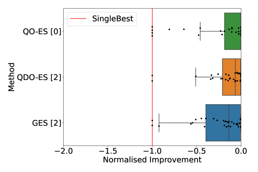
(a) ROC AUC - Binary (41 Datasets)

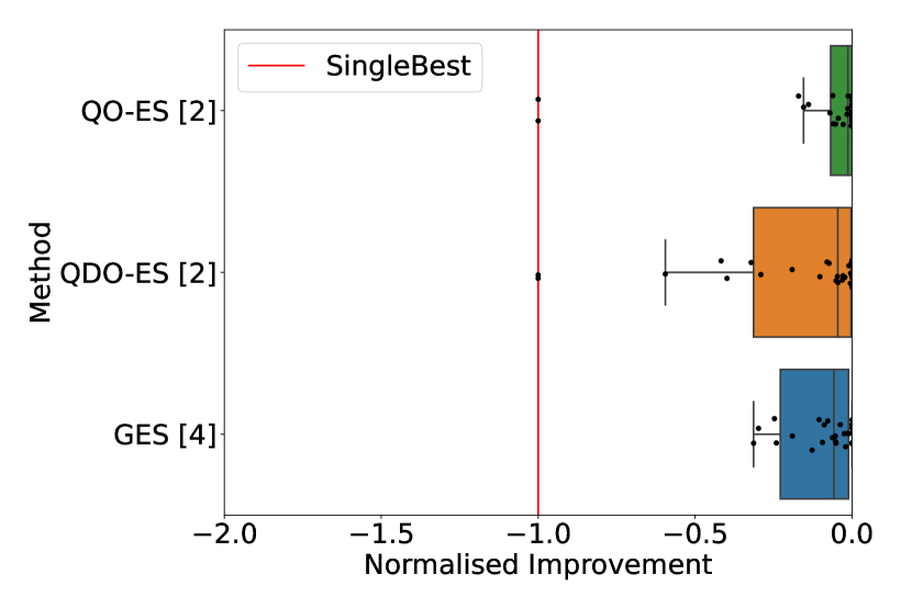
(b) ROC AUC - Multi-class (30 Datasets)

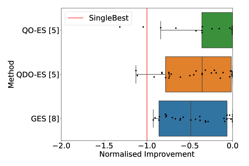
(c) Balanced Accuracy - Binary (41 Datasets)

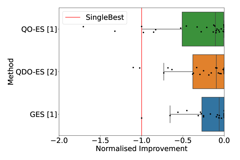
(d) Balanced Accuracy - Multi-class (30 Datasets)

Figure 2: Normalised Improvement Boxplots: Higher is better. Each dot represents a dataset. The number in square brackets next to a method’s name counts the outliers smaller than $-2$.

We want to note that computing all results without parallelization across datasets, folds, configurations, and metrics but with parallelization of the AutoML systems and the ensemble method on 8 cores took approximately around $3.9$ years of wall-clock time, see Appendix F.1.

Overfitting

We observed that overfitting had a large influence on the final testing performance of our methods when repeating our evaluation for validation instead of testing scores; see Figure 3. We note that the difference between Q(D)O-ES and GES is statistically significant in all scenarios. Moreover, the normalised improvement gains for Q(D)O-ES are also substantially larger than for GES, see Appendix F.2. Likewise, as expected, no post hoc ensembling method performs worse than the single best model on any dataset. Thus, the main challenge post hoc ensembling encounters is the lack of generalisation from validation to testing sets.

(a) ROC AUC - Binary (41 Datasets)

(b) ROC AUC - Multi-class (30 Datasets)

(c) Balanced Accuracy - Binary (41 Datasets)

(d) Balanced Accuracy - Multi-class (30 Datasets)

Figure 3: Critical Difference Plots for Validation Scores: Mean rank of the methods (lower is better). Methods connected by a bar are not significantly different.

We believe that the validation data generated by Auto-Sklearn’s 33% hold-out split may be responsible for the large difference between validation and test performance. In future work, it would be interesting to investigate the performance and generalisation of our methods for other AutoML systems that use more sophisticated validation procedures, e.g., AutoGluon with n-repeated k-fold cross-validation.

Regarding GES, we observe that based on the LOO CV procedure, AutoGluon’s variant is always selected for balanced accuracy, while for ROC AUC, Auto-Sklearn’s variant is selected for all multi-class classification datasets and ${\sim}12\%$ ($5/41$) binary classification datasets. For validation scores, AutoGluon’s variant is always selected. We note that the difference in the implementations of AutoGluon and Auto-Sklearn (see Section 2) can be interpreted as differences in handling overfitting: the first variant is more prone to overfitting than the latter, due to relying more on the validation score for the selection of the final ensemble.

Ensemble Diversity

We note that for all methods, the preprocessing approach selected based on the LOO CV procedure was SiloTopN, rather than TopN. The diversity of base models fostered by including algorithms from each family seems to always be beneficial. This difference in algorithmic diversity is also visible in the pool of base models $P$ per dataset. The average number of distinct algorithms in $P$ across all datasets and metrics is ${\sim}2.77$ for TopN while SiloTopN achieves ${\sim}15.33$; see Table 2 in Appendix E.1 for numbers per dataset. We also observe this when analysing hyperparameter importance, see Appendix F.3; we found the preprocessing method to be the most important hyperparameter, followed by the sampling and initialisation method.

Regarding the use of ensemble diversity for optimisation, we see that QO-ES beats QDO-ES except for balanced accuracy multi-class on testing data. On validation data, QDO-ES always beats QO-ES, although the differences in rank are not significant. We hypothesise that adding ensemble diversity to the optimisation process can, in principle, be beneficial, but also increases the risk of overfitting, because it utilises the distribution of ensemble diversity, which might not generalise.

Efficiency

See Table 1 for an overview of the efficiency for each ensemble method per scenario. The size of an ensemble corresponds to how many base models must compute predictions and thus directly represents the inference efficiency of an ensemble. To investigate the optimisation efficiency of the methods we studied, we looked at the average running time required for completing $50$ iterations. Note that for multi-class, the methods are more efficient for balanced accuracy than for ROC AUC, as computing balanced accuracy is more costly than ROC AUC for multi-class.

The average size across all scenarios of the generated ensembles is ${\sim}8.5$ for GES, ${\sim}12$ for QO-ES, and ${\sim}12$ for QDO-ES. Although Q(D)O-ES generates slightly bigger ensembles, their weight vectors are still sparse, considering that $50$ base models were available in most cases. GES needs on average across all scenarios ${\sim}103$ seconds. Our current implementation of QO-ES takes ${\sim}165$ seconds, and QDO-ES ${\sim}196$ seconds, but optimising our code would likely increase efficiency. We note that these times are insignificant compared to the time budget of $4$ hours expended by Auto-Sklearn for finding the base models.

Table 1: Ensemble Efficiency: Average ensemble size and running time for $50$ iterations in seconds.

	Average Ensemble Size				Average Running Time $@50$
	Balanced Accuracy		ROC AUC		Balanced Accuracy		ROC AUC
Method	Binary	Multi-class	Binary	Multi-class	Binary	Multi-class	Binary	Multi-class
GES	7.95	7.91	8.02	10.09	49.13	120.36	43.66	197.57
QDO-ES	9.23	11.47	14.06	13.27	81.92	158.24	91.04	451.48
QO-ES	8.02	10.28	15.76	13.88	65.41	132.76	75.5	388.62

Ablation Study

When performing ablation studies for Q(D)O-ES, we found that the preprocessing approach seems to be the most important component for our approach; followed by the sampling method and approach of archive initialisation (see Appendix F.3). Specifically, SiloTopN seems to always perform better than TopN, as indicated by the selected preprocessing approach above (see Appendix F.4). The best sampling and initialisation method seem to differ slightly per scenario.

7  Conclusion

Post hoc ensembling is widely used in AutoML systems and can be crucial for obtaining peak predictive performance. One of the most popular methods is greedy ensemble selection with replacement (GES) (Caruana et al.,, 2004, 2006). In this work, we presented QO-ES and QDO-ES, two novel population-based optimisation algorithms for post hoc ensemble selection in AutoML. QO-ES maintains an archive of the best-performing ensembles and sequentially improves upon them, making use of mutation and crossover operators. QDO-ES builds upon QO-ES, but leverages concepts from quality diversity optimisation (Chatzilygeroudis et al.,, 2021), maintaining an archive of differently behaviourally diverse ensembles during optimisation. In extensive experiments, we demonstrated that 1) post hoc ensemble selection improves upon the single best model, 2) our population-based methods QO-ES and QDO-ES generally outperform GES (although the performance differences are not statistically significant on testing data), and 3) respecting the diversity of ensembles during optimisation can be beneficial but also increases the risk of overfitting. Lastly, we want to highlight that overfitting is a serious challenge for post hoc ensembling in AutoML.

Acknowledgements

The CPU nodes of the OMNI cluster of the University of Siegen (North Rhine-Westphalia, Germany) were used for all experiments presented in this work. This research is partially supported by the Bavarian Ministry of Economic Affairs, Regional Development and Energy through the Center for Analytics - Data - Applications (ADACenter) within the framework of BAYERN DIGITAL II (20-3410-2-9-8) and by TAILOR, which is part of the EU Horizon 2020 research and innovation programme under GA No 952215. Finally, we thank the reviewers for their constructive feedback and contribution to improving the paper.

Appendix A Submission Checklist

1. For all authors…

   1. Do the main claims made in the abstract and introduction accurately reflect the paper’s contributions and scope? [Yes] We state in the abstract and introduction that we compare GES to QO-ES and QDO-ES, which is what we did in the paper.

   2. Did you describe the limitations of your work? [Yes] In the Appendix, see B.

   3. Did you discuss any potential negative societal impacts of your work? [Yes] In the Appendix, see C.

   4. Have you read the ethics author’s and review guidelines and ensured that your paper conforms to them? https://2023.automl.cc/ethics/ [Yes] We believe our paper confirms to them.

2. If you are including theoretical results…

   1. Did you state the full set of assumptions of all theoretical results? [N/A] We included no theoretical results.

   2. Did you include complete proofs of all theoretical results? [N/A] We included no theoretical results.

3. If you ran experiments…

   1. Did you include the code, data, and instructions needed to reproduce the main experimental results, including all requirements (e.g., requirements.txt with explicit version), an instructive README with installation, and execution commands (either in the supplemental material or as a url)? [Yes] See our repository mentioned in the introduction for all details.

   2. Did you include the raw results of running the given instructions on the given code and data? [Yes] See our repository mentioned in the introduction for the results.

   3. Did you include scripts and commands that can be used to generate the figures and tables in your paper based on the raw results of the code, data, and instructions given? [Yes] See our repository mentioned in the introduction.

   4. Did you ensure sufficient code quality such that your code can be safely executed and the code is properly documented? [Yes] We believe that our code quality and documentation are sufficient.

   5. Did you specify all the training details (e.g., data splits, pre-processing, search spaces, fixed hyperparameter settings, and how they were chosen)? [Yes] See the Section 5 and the Appendix for detail. Additionally, see our repository mentioned in the introduction.

   6. Did you ensure that you compared different methods (including your own) exactly on the same benchmarks, including the same datasets, search space, code for training and hyperparameters for that code? [Yes] We ran all methods on the same data.

   7. Did you run ablation studies to assess the impact of different components of your approach? [Yes] We ran our approach for a gird of hyperparameters and assessed their importance, see Appendix E.2 and F.3.

   8. Did you use the same evaluation protocol for the methods being compared? [Yes] We ran all methods on the same data with the same evaluation protocol and code.

   9. Did you compare performance over time? [No] We compared performance for a specific point in time (after $50$ iterations of GES, i.e., after $m*50$ function evaluations). Performance over time was out of scope for our experiments. In our opinion, anytime performance is much less relevant for post hoc ensembling compared to other AutoML methods such as HPO or NAS.

   10. Did you perform multiple runs of your experiments and report random seeds? [Yes] Yes, we used 10-fold cross-validation for all our runs. The used random seeds can be found in our code.

   11. Did you report error bars (e.g., with respect to the random seed after running experiments multiple times)? [No] We took the average over the 10 folds as a score following previous work and have not reported variance across folds. Nevertheless, boxplots allow for assessing the variance of performance with respect to different data sets.

   12. Did you use tabular or surrogate benchmarks for in-depth evaluations? [N/A] Such benchmarks were not available for our use case.

   13. Did you include the total amount of compute and the type of resources used (e.g., type of gpus, internal cluster, or cloud provider)? [Yes] See Section 5.

   14. Did you report how you tuned hyperparameters, and what time and resources this required (if they were not automatically tuned by your AutoML method, e.g. in a nas approach; and also hyperparameters of your own method)? [Yes] See Section 5.

4. If you are using existing assets (e.g., code, data, models) or curating/releasing new assets…

   1. If your work uses existing assets, did you cite the creators? [Yes] See Section 5 and Appendix G.

   2. Did you mention the license of the assets? [Yes] See Appendix G.

   3. Did you include any new assets either in the supplemental material or as a url? [Yes] See our repository mentioned in the introduction.

   4. Did you discuss whether and how consent was obtained from people whose data you’re using/curating? [N/A] We are only using publicly available data that was used before in benchmarks.

   5. Did you discuss whether the data you are using/curating contains personally identifiable information or offensive content? [N/A] We believe that the data we are using does not contain personally identifiable information or offensive content.

5. If you used crowdsourcing or conducted research with human subjects…

   1. Did you include the full text of instructions given to participants and screenshots, if applicable? [N/A] We did not use crowdsourcing or conducted research with human subjects.

   2. Did you describe any potential participant risks, with links to Institutional Review Board (irb) approvals, if applicable? [N/A] We did not use crowdsourcing or conducted research with human subjects.

   3. Did you include the estimated hourly wage paid to participants and the total amount spent on participant compensation? [N/A] We did not use crowdsourcing or conducted research with human subjects.

Appendix B Limitations

We note that our work is limited with respect to the following points: 1) we found that overfitting is a large problem but only were able to compare our methods for Auto-Sklearn 1 and not additional AutoML systems that have better validation data available, such as Auto-Sklearn 2 or AutoGluon; 2) we were only able to explore a subset of all possible hyperparameters and hyperparameter settings for our newly proposed methods; 3) we were only able to evaluate w.r.t. two metrics; and 4) we were not able to explore all potential variations of QDO that could have been used for QDO-ES.

Appendix C Broader Impact Statement

We believe that our work is mostly abstract and methodical. Thus, after careful reflection, we determined that this work presents no notable or new negative impacts to society or the environment that are not already present for existing state-of-the-art AutoML systems. We proposed to replace one component of an AutoML system such that the predictive performance improves while efficiency stays mostly the same. Therefore, we only see the potential positive impact that higher predictive performance might help to make better decisions using AutoML.

Appendix D Supplements for the Algorithm Description

D.1  Formula for Diversity Measures

To measure the diversity of an ensemble $E=(P,r)$, we consider all non-zero weighted base models in the ensemble, that is, $P^{\prime}=\{p_{i}\in P\;|\;r(i)>0\}$ with $|P^{\prime}|=m^{\prime}$.

The average loss correlation (ALC) is defined for $P^{\prime}$ and a set of loss vectors $L=\{l_{1},...,l_{m^{\prime}}\}$. A loss vector $l_{i}$ corresponds to the difference between $1$ and the prediction probability of $p_{i}$ for the correct class for each instance. Then, ALC is defined as the average Pearson correlation $\rho$ of two loss vectors over all pairs of models in $P^{\prime}$:

$$ALC=\frac{2}{m^{\prime}(m^{\prime}-1)}\sum^{m^{\prime}-1}_{i=1}\sum^{m^{\prime}}_{j=i+1}\rho(l_{i},l_{j}).$$ (2)

The configuration space similarity (CSS) is defined for $P^{\prime}$ and a set of configurations $C=\{c_{1},...,c_{m^{\prime}}\}$ where $c_{i}$ is the configuration of $p_{i}$. We assume that the configurations are from the same configuration space such that at least the hyperparameter describing the used algorithm exists for any two $c$. Moreover, we assume that we are given the maximal observed ranges in $C$ of all numerical hyperparameters. For a numerical hyperparameter $h$, we denote its range with $R_{h}$. Generally, we denote the value of a configuration $c$ for a hyperparameter $h$ with $h^{c}$. CSS is the average Gower distance (Gower,, 1971) over all pairs of models in $P^{\prime}$:

$$CSS=\frac{2}{m^{\prime}(m^{\prime}-1)}\sum^{m^{\prime}-1}_{i=1}\sum^{m^{\prime}}_{j=i+1}(1-G_{i,j}).$$ (3)

The Gower similarity $G_{i,j}$ is defined only for the set of hyperparameters $K=\{h_{1},...,h_{|K|}\}$ that appear in $c_{i}$ and $c_{j}$. Furthermore, the Gower similarity differentiates between categorical and numeric hyperparameters and is the average over the similarity of each hyperparameter in $K$:

$$G_{i,j}=\frac{1}{|K|}\sum_{k=1}^{|K|}\begin{cases}G^{\mathrm{cat}}_{i,j,k},&\mbox{if $h_{k}$ is categorical}\\ G^{\mathrm{num}}_{i,j,k},&\mbox{otherwise}\end{cases},$$ (4)

with

$$G^{\mathrm{cat}}_{i,j,k}=\begin{cases}\mbox{1,}&\mbox{if }h_{k}^{c_{i}}=h_{k}^{c_{j}}\\ \mbox{0,}&\mbox{otherwise}\end{cases},$$ (5)

and,

$$G^{\mathrm{num}}_{i,j,k}=\frac{|h^{c_{i}}_{k}-h^{c_{j}}_{k}|}{R_{h_{k}}}.$$ (6)

As at least the hyperparameter describing the used algorithm exits for both configurations, $G_{i,k}\geq 0$. Moreover, it is at most $1$ if all hyperparameters are identical.

D.2  Motivation to use a Sliding Boundaries Archive for QDO-ES

For QDO-ES, we implemented a sliding boundaries archive (Fontaine et al.,, 2019). A sliding boundaries archive regularly recomputes the niche boundaries based on the observed range of behaviour values after initialising the niches based on the theoretical range.

We use a sliding boundaries archive because we cannot guarantee that the observable values of a behaviour space for ensemble diversity are uniformly distributed, as is usually assumed for QDO (Chatzilygeroudis et al.,, 2021; Nickerson and Hu,, 2021). Moreover, the observable range of ensemble diversity metrics differs between datasets since they depend, e.g., on the base models’ predictions. The sliding boundaries archive allows us to maintain a similar granularity of the partitions between datasets. The granularity will also be finer than the initially computed partitions and thus enable more local competition.

Additionally and more importantly, because we keep one ensemble per niche, the sliding boundaries archive aligns the population with the underlying distribution of the observed behaviour space, making random sampling more representative.

D.3  Used Variant of Tournament Selection

In our non-deterministic variant of tournament selection, we define the tournament size $T$ based on the number of solutions we want to sample. If we want to sample one solution, we randomly sample 10 solutions from the archive. We sample 20 solutions if we want to sample two solutions. In the first few iterations, we might have less than $T$ solutions in the archive. In such a case, we take all solutions in the archive and additionally mutate solutions, taken from the initial set of solutions proposed to the archive, with Algorithm 3.

Given $T$-many solutions, we assign each solution a probability of being sampled. The best-performing solution is assigned a probability of $0.8$, the second best $0.8*0.2^{1}$, the third best $0.8*0.2^{2}$, and so on until $0.8*0.2^{(T-1)}$. Finally, we sample either one or two solutions with these probabilities. If we sample two solutions, we sample without replacement.

D.4  Implementation of an Adaptive Probability

We have several components in our algorithm where a probability defines whether these are activated or deactivated or how they are configured. In all cases, we used a self-adaptive probability instead of a predetermined constant value or function over time. Thus, avoiding additional hyperparameters and the bias of selecting a constant value or function over time for all tasks. This includes: dynamic sampling; whether crossover is used; and whether mutation is used after crossover.

We can represent such a choice as a binary decision between using $a$ or $b$. Initially, the probability of using $a$, $Pr(a)$, is set to $50\%$ (consequently $Pr(b)=1-Pr(a)$). That is, we randomly select whether to use $a$ or $b$. Then, after each iteration, the probability is adapted based on the observed performance of $a$ and $b$ over the last $f$ iterations. $f$ is a hyperparameter. We set $f=10$ because we aimed for a window over the performance such that bad performance in earlier iterations can be forgotten in face of dynamic changes to the performance of $a$ and $b$. We track the performance of solutions in relation to their origin, i.e., whether the solutions were produced with $a$ or $b$. Moreover, we do not change the probability if less than $2$ solutions were created with $a$ or $b$.

For the update, we first compute the average performance over all solutions seen in the last $10$ iterations for $a$ and $b$, denoted as $a_{avg}$ and $b_{avg}$. Using these values, we compute: $Pr(a)=1-\frac{a_{avg}}{a_{avg}+b_{avg}}$. Finally, we bound $Pr(a)$ in $\left[0.05,0.95\right]$ for dynamic sampling and in $\left[0.1,0.9\right]$ otherwise. We apply these bounds to avoid reaching a probability of $0$ for $a$ or $b$ such that it would not be chosen anymore and consequently not have solutions for an update.

We have tighter bounds for mutation after crossover and crossover, since we observed that a probability of $0.05$ behaved similarly to a probability of $0$ – not enough solutions were produced such that future updates could change the probability. This happens only for mutation after crossover and crossover, as both are only used for a subset of all solutions. In contrast, dynamic sampling is always used as the initial step for creating a new solution (see Algorithm 2); assuming dynamic sampling is used and not another sampling method.

D.5  Mutation Operator

Our mutation operator follows the idea of GES (Algorithm 1), in the sense that we adjust $r$ during mutation by incrementing one of its elements. We introduce additional stochasticity by randomly choosing this element. Consequently, we implemented a randomized version of GES’s update as a mutation operator, see Algorithm 3. However, since $E$ is not built iteratively in Q(D)O-ES, we need to track which base model we previously added to avoid producing the same ensemble twice (handled by lines 4, 7, and 8).

Algorithm 3 Iteration Independent Randomized With-replacement-like Mutation

1:Ensemble $E=(P,r)$

2:Ensemble $E_{mutated}=(P,r_{mutated})$

3:$R\leftarrow\{r^{\prime}\;|\;r^{\prime}=r\text{ with one element incremented by $1$}\}$ $\triangleright$ Obtain all possible extensions of $r$

4:$R_{seen}\leftarrow lookUpSeenFor(r)$ $\triangleright$ Obtain previously produced extensions

5:$R_{potential}\leftarrow R\setminus R_{seen}$

6:$r_{mutated}\leftarrow randomSample(R_{potential})$

7:$R_{seen}\leftarrow R_{seen}\cup r_{mutated}$ $\triangleright$ Update previously produced extensions

8:$storeForLookUp(r,R_{seen});storeForLookUp(r_{mutated},\emptyset)$ $\triangleright$ Store previously produced extensions

9:return $(P,r_{mutated})$

D.6  Two-Point Crossover of Repetition Vectors

For two-point crossover of two repetition vectors $r$ and $r^{\prime}$, we first select the subsets $r_{sub}$ and $r_{sub}^{\prime}$ of elements that are non-zero in either $r$ or $r^{\prime}$. If this subset is smaller than three, we fall back to average crossover. We require a vector of at least length three to perform two-point crossover. Otherwise, only one possibility to perform two-point crossover would exist.

Next, we select two distinct points randomly and crossover $r_{sub}$ and $r_{sub}^{\prime}$ with these points. Afterwards, we fill $r$ / $r^{\prime}$ with the elements of $r_{sub}$ / $r_{sub}^{\prime}$ creating $r_{co}$ / $r_{co}^{\prime}$. Finally, we verify that the elements of $r_{co}$ / $r_{co}^{\prime}$ are not all zero and return $r_{co}$ / $r_{co}^{\prime}$. If neither $r_{co}$ nor $r_{co}^{\prime}$ contain non-zero elements, then we again fall back to average crossover to produce offspring.

Two-point crossover can produce two unique children. If this happens, we add both (mutated) children to the batch in QO-ES and QDO-ES (Algorithm 2).

D.7  Initialisation Approaches

Population-based search requires an initial population $S$. To produce the initial population for Q(D)O-ES, we implemented three approaches: all ensembles consisting only of a base model, all ensembles of size $2$ including the best base model, or $m$-many random ensembles of size $2$. Formally, the set of all ensembles consisting only of one base model is given by

$$S_{1}=\biggl{\{}(P,r)\;\bigg{|}\;\sum^{m}_{i=1}r(i)=1\biggr{\}}.$$ (7)

The set of all ensembles of size $2$ including the best base model with $j$ the index of the single best model, is given by

$$S_{2}=\biggl{\{}(P,r)\;\bigg{|}\;r(j)=1\wedge\sum^{m}_{i=1}r(i)=2\biggr{\}}.$$ (8)

The single best model is the base model in $P$ with the highest validation score. To construct the set $S_{3}$ of $m$-many random ensembles of size $2$, we randomly select two members of the ensemble $m$ times. Formally, $S_{3}\subset\hat{S}_{3}$ with $|S_{3}|=m$ and $\hat{S}_{3}$ the set of all possible ensembles of size $2$:

$$\hat{S}_{3}=\biggl{\{}(P,r)\;\bigg{|}\;\exists!i,j\in\{1,\ldots,m\},i\neq j:r(i)=1=r(j)\ \biggr{\}}.$$ (9)

Note, the size of this initial population differs between the methods by definition; $S_{1}=S_{3}=m$ while $S_{2}=m-1$.

D.8  Emergency Brake for Rejection Sampling

We added an emergency brake that temporarily changes the increment during mutations (Algorithm 3, Line 3) and/or probability of crossover when more than $50$ solutions are rejected in one iteration.

We were motivated to do this because we observed an edge case where Algorithm 2 was not able to propose any unseen solutions. Thus, the algorithm ran into an endless loop of rejection sampling. We observed this in the first few iterations of the algorithm after the archive was initialised with ensembles consisting only of a base model, or when the probability of crossover was very high in the first few iterations.

Our overall emergency brake consists of two parts, one brake for rejections resulting from mutation and one for rejections resulting from crossover. In one iteration, both brakes can be activated (multiple) times at the same time if the algorithm still does not produce unseen solutions.

If mutation does not produce any new solutions and crossover is deactivated (or does not produce new solutions either), then the mutation emergency brake is activated after $50$ rejections resulting from mutation. Once the break is activated, the increment of the repetition vectors during mutation (Algorithm 3, Line 3) is increased by $1$ for the current iteration.

The rejections might also result from solutions created by crossover and not by mutation because crossover cannot produce unseen children, and the adaptive probability of mutation after crossover is too small to be called in the current iteration. In this case, we increase the probability of mutation after crossover to $100\%$ for this iteration after $50$ rejections stemming from crossover.

Appendix E Supplements for the Experiments

E.1  Dataset Overivew

Table 2 gives an overview of datasets and base models used in our experiments. Additionally, we show the average (over folds) for the number of base models and the number of distinct algorithms over the pools of base models for balanced accuracy $\mathcal{BA}$ and ROC AUC $\mathcal{R}$, respectively for the preprocessing methods SiloTopN and TopN.

Table 2: Supplementary information for all datasets and generated base models.

Dataset Name						Mean #Base Models				Mean #Distinct Algorithms
	OpenML Task ID	#Instances	#Features	#Classes	Memory (GB)	$\mathcal{BA}_{TopN}$	$\mathcal{BA}_{SiloTopN}$	$\mathcal{R}_{TopN}$	$\mathcal{R}_{SiloTopN}$	$\mathcal{BA}_{TopN}$	$\mathcal{BA}_{SiloTopN}$	$\mathcal{R}_{TopN}$	$\mathcal{R}_{SiloTopN}$
yeast	2073	1484	9	10	32	50.0	50.0	50.0	50.0	1.7	16.0	2.1	16.0
KDDCup09_appetency	3945	50000	231	2	32	50.0	50.0	50.0	50.0	1.5	16.0	1.2	15.8
covertype	7593	581012	55	7	64	49.9	49.9	50.0	50.0	10.0	12.6	7.9	12.2
amazon-commerce-reviews	10090	1500	10001	50	32	50.0	50.0	50.0	50.0	1.4	15.8	1.8	15.9
Australian	146818	690	15	2	32	50.0	50.0	50.0	50.0	2.8	16.0	2.3	16.0
wilt	146820	4839	6	2	32	50.0	50.0	50.0	50.0	1.3	16.0	1.6	16.0
numerai28.6	167120	96320	22	2	32	50.0	50.0	50.0	50.0	5.3	15.8	5.0	15.7
phoneme	168350	5404	6	2	32	50.0	50.0	50.0	50.0	1.3	16.0	1.3	16.0
credit-g	168757	1000	21	2	32	50.0	50.0	50.0	50.0	1.5	16.0	2.6	16.0
steel-plates-fault	168784	1941	28	7	32	50.0	50.0	50.0	50.0	1.4	16.0	1.1	16.0
APSFailure	168868	76000	171	2	32	50.0	50.0	50.0	50.0	2.5	16.0	2.0	16.0
dilbert	168909	10000	2001	5	32	50.0	50.0	50.0	50.0	1.5	15.7	1.0	15.7
fabert	168910	8237	801	7	32	50.0	50.0	50.0	50.0	3.4	16.0	2.6	16.0
jasmine	168911	2984	145	2	32	50.0	50.0	50.0	50.0	3.0	15.8	1.9	15.9
airlines	189354	539383	8	2	64	50.0	50.0	50.0	50.0	5.8	14.5	5.9	14.4
dionis	189355	416188	61	355	128	20.8	20.8	28.2	28.2	7.4	7.4	7.9	7.9
albert	189356	425240	79	2	64	50.0	50.0	50.0	50.0	8.1	13.6	8.6	12.5
gina	189922	3153	971	2	32	50.0	50.0	50.0	50.0	1.0	16.0	1.0	16.0
ozone-level-8hr	190137	2534	73	2	32	50.0	50.0	50.0	50.0	1.0	16.0	1.8	15.9
vehicle	190146	846	19	4	32	50.0	50.0	50.0	50.0	1.6	16.0	1.6	16.0
madeline	190392	3140	260	2	32	50.0	50.0	50.0	50.0	1.2	16.0	1.3	16.0
philippine	190410	5832	309	2	32	50.0	50.0	50.0	50.0	1.0	16.0	1.2	16.0
ada	190411	4147	49	2	32	50.0	50.0	50.0	50.0	1.9	16.0	1.6	16.0
arcene	190412	100	10001	2	32	50.0	50.0	50.0	50.0	1.3	16.0	1.2	15.9
jannis	211979	83733	55	4	32	50.0	50.0	50.0	50.0	1.0	15.4	3.1	15.1
Diabetes130US	211986	101766	50	3	32	50.0	50.0	50.0	50.0	1.0	15.6	1.0	15.7
micro-mass	359953	571	1301	20	32	50.0	50.0	50.0	50.0	1.1	16.0	1.5	16.0
eucalyptus	359954	736	20	5	32	50.0	50.0	50.0	50.0	1.3	16.0	2.6	15.9
blood-transfusion-service-center	359955	748	5	2	32	50.0	50.0	50.0	50.0	1.9	16.0	4.1	16.0
qsar-biodeg	359956	1055	42	2	32	50.0	50.0	50.0	50.0	2.4	16.0	2.3	16.0
cnae-9	359957	1080	857	9	32	50.0	50.0	50.0	50.0	1.6	16.0	1.2	16.0
pc4	359958	1458	38	2	32	50.0	50.0	50.0	50.0	1.4	16.0	2.1	16.0
cmc	359959	1473	10	3	32	50.0	50.0	50.0	50.0	1.9	16.0	1.6	16.0
car	359960	1728	7	4	32	50.0	50.0	50.0	50.0	1.1	16.0	1.0	16.0
mfeat-factors	359961	2000	217	10	32	50.0	50.0	50.0	50.0	1.1	16.0	3.5	16.0
kc1	359962	2109	22	2	32	50.0	50.0	50.0	50.0	2.2	16.0	2.2	16.0
segment	359963	2310	20	7	32	50.0	50.0	50.0	50.0	1.4	16.0	1.4	16.0
dna	359964	3186	181	3	32	50.0	50.0	50.0	50.0	1.2	16.0	1.1	15.8
kr-vs-kp	359965	3196	37	2	32	50.0	50.0	50.0	50.0	1.8	16.0	1.1	15.8
Internet-Advertisements	359966	3279	1559	2	32	50.0	50.0	50.0	50.0	1.8	16.0	2.6	16.0
Bioresponse	359967	3751	1777	2	32	50.0	50.0	50.0	50.0	3.6	15.9	2.6	15.8
churn	359968	5000	21	2	32	50.0	50.0	50.0	50.0	1.3	16.0	1.2	16.0
first-order-theorem-proving	359969	6118	52	6	32	50.0	50.0	50.0	50.0	2.8	15.8	2.6	15.7
GesturePhaseSegmentationProcessed	359970	9873	33	5	32	50.0	50.0	50.0	50.0	1.1	15.8	2.0	15.9
PhishingWebsites	359971	11055	31	2	32	50.0	50.0	50.0	50.0	1.1	15.8	1.1	15.6
sylvine	359972	5124	21	2	32	50.0	50.0	50.0	50.0	1.3	16.0	1.1	16.0
christine	359973	5418	1637	2	32	50.0	50.0	50.0	50.0	3.5	15.8	2.9	15.9
wine-quality-white	359974	4898	12	7	32	50.0	50.0	50.0	50.0	1.0	16.0	1.7	16.0
Satellite	359975	5100	37	2	32	50.0	50.0	50.0	50.0	1.2	16.0	1.2	16.0
Fashion-MNIST	359976	70000	785	10	64	50.0	50.0	50.0	50.0	12.3	13.4	6.1	15.0
connect-4	359977	67557	43	3	32	50.0	50.0	50.0	50.0	1.0	16.0	1.0	15.7
Amazon_employee_access	359979	32769	10	2	32	50.0	50.0	50.0	50.0	2.5	15.9	1.7	16.0
nomao	359980	34465	119	2	32	50.0	50.0	50.0	50.0	1.0	15.9	1.0	15.9
jungle_chess_2pcs_raw_endgame_complete	359981	44819	7	3	32	50.0	50.0	50.0	50.0	1.0	16.0	1.0	16.0
bank-marketing	359982	45211	17	2	32	50.0	50.0	50.0	50.0	1.0	15.8	1.2	15.8
adult	359983	48842	15	2	32	50.0	50.0	50.0	50.0	1.3	16.0	1.0	16.0
helena	359984	65196	28	100	32	50.0	50.0	50.0	50.0	2.8	15.8	3.6	15.2
volkert	359985	58310	181	10	32	50.0	50.0	50.0	50.0	2.1	15.5	1.1	15.5
robert	359986	10000	7201	10	64	50.0	50.0	50.0	50.0	11.2	14.3	7.7	13.7
shuttle	359987	58000	10	7	32	50.0	50.0	50.0	50.0	1.2	16.0	2.1	16.0
guillermo	359988	20000	4297	2	32	50.0	50.0	50.0	50.0	3.1	15.5	2.9	15.6
riccardo	359989	20000	4297	2	32	50.0	50.0	50.0	50.0	1.5	15.6	1.1	15.5
MiniBooNE	359990	130064	51	2	32	50.0	50.0	50.0	50.0	1.4	15.7	1.1	15.4
kick	359991	72983	33	2	32	50.0	50.0	50.0	50.0	2.0	15.9	1.2	15.8
Click_prediction_small	359992	39948	12	2	32	50.0	50.0	50.0	50.0	1.0	16.0	1.0	15.9
okcupid-stem	359993	50789	20	3	32	50.0	50.0	50.0	50.0	1.1	15.9	1.0	15.5
sf-police-incidents	359994	2215023	9	2	64	49.5	49.5	50.0	50.0	10.5	12.9	6.1	13.1
KDDCup99	360112	4898431	42	23	128	13.5	13.5	29.2	29.2	5.1	5.1	9.2	9.2
porto-seguro	360113	595212	58	2	64	50.0	50.0	50.0	50.0	10.6	14.4	10.8	14.5
Higgs	360114	1000000	29	2	64	47.9	47.9	48.8	48.8	9.8	13.2	11.2	11.8
KDDCup09-Upselling	360975	50000	14892	2	128	50.0	50.0	49.0	49.0	4.9	13.4	6.0	11.7

E.2  Configuration Space

Table 3 shows all hyperparameter and their possible values for the configuration space of QO-ES and QDO-ES. We refer to the set of all ensembles consisting only of a single base model as L1 Ensembles, while we refer to all ensembles of size $2$ that include the single best model, or $m$-many random ensembles of size $2$ as L2 Ensembles.

Table 3: Q(D)O-ES Configuration Space.

Hyperparameter	Values
Preprocessing	SiloTopN, TopN
Batch Size	20, 40
Archive Size	16, 49
Archive Initialisation	L1 Ensembles, L2 of Single Best, Random L2
Sampling Method	Deterministic, Tournament, Dynamic
Crossover	two-point crossover, average crossover, no crossover

E.3  Discussion on the Configuration Selection Approach

We use the median normalised improvement to select the most representative configuration during leave-one-out cross-validation because it reflects what we believe to be the distinguishing factor between different methods based on an evaluation following the AutoML benchmark (AMLB) (Gijsbers et al.,, 2022) – the highest median in the boxplots of the normalised improvement.

We are aware that alternative selection approaches could change our results or that one could, in principle, learn to select the best configuration. However, the only valid alternative in an evaluation following the AMLB would have been mean rank. As this is the only other distinguishing factor used in plots, specifically critical difference plots. However, as noted already in the AMLB and visible in its results, the absolute rank is not representative of a performance distribution and hides relative performance differences. In contrast, the median normalised improvement is based on a relative measure and relates to a performance distribution via the median.

E.4  Normalised Improvement

Our implementation of normalised improvement follows the AutoML benchmark (Gijsbers et al.,, 2022). That is, we scale the scores for a dataset such that $-1$ is equal to the score of the single best model, and $0$ is equal to the score of the best method on the dataset.

Formally, we normalise the score $s_{D}$ of a method for a dataset $D$ using:

$$\frac{s_{D}-s_{D}^{b}}{s_{D}^{*}-s_{D}^{b}}-1,$$ (10)

with the score of the baseline $s_{D}^{b}$ and the best-observed score for the dataset $s_{D}^{*}$. We assume that higher scores are always better.

We extend this definition for the edge cases where no method is better than the baseline, i.e., $s_{D}^{*}-s_{D}^{b}=0$. We assume that this edge case never happened in the AutoML benchmark. Otherwise, their definition and implementation would have been undefined / crashed. In our setting, such an edge case can happen due to overfitting such that the ensemble methods becomes worse than the single best model.

We generalize the definition of this edge case to the case $|s_{D}^{*}-s_{D}^{b}|<=\Delta$. We set $\Delta$ to $0.0001$, because normalised improvement also becomes unrepresentative for a dataset if $s_{D}^{*}-s_{D}^{b}$ is very small (because we divide by $s_{D}^{*}-s_{D}^{b}$).

If the edge case happens, we set the score of all methods worse than the baseline to $-10$, following a penalization-like approach (e.g., PAR10 from Algorithm Selection (Lindauer et al.,, 2019)). Methods for which $|s_{D}-s_{D}^{b}|<=\Delta$ holds are assigned a score of $-1$.

Appendix F Supplements for the Results

F.1  Estimated Lower Bound of Wall-Clock Time for the Experiments

We estimated the lower bound for the wall-clock time for our experiments to be approximately $3.91$ years. We did not capture the CPU time while running our experiments and cannot calculate this in retrospect due to parallelization. We note, that the wall-clock time is an absolute lower bound for the CPU time. Moreover, for our estimate of wall-clock time, we exclude the overhead that parallelization and containerization induced, because we did not time this overhead. Nevertheless, we believe this to be a non-marginal overhead, considering the considerable number of ensemble runs and our experiences of running the experiments.

To compute the estimate, we first consider the wall-clock time it took to generate the base models with Auto-Sklearn. Therefore, we multiply the budget of $4$ hours that we gave to Auto-Sklearn with 8 cores: $4$ hours $\times$ $10$ folds $\times$ $71$ datasets $\times$ $2$ metrics; amounting to ${\sim}0.65$ years.

Next, we consider the wall-clock time it took to run all configurations of all ensemble methods. Therefore, we use the time it took to fit and predict with the ensemble methods. We captured this while evaluating the ensemble methods (the related data can be found in our code repository). Note, that the fit and predict time measurement excludes any time spent related to the base models, as the evaluation only works on predictions of the base models stored after their generation – this excludes loading the predictions or the datasets. Likewise, the measured time excludes the time it took to score ensemble methods and store the results related to the evaluation. Lastly, the ensemble method had 8 cores available for fitting and predicting. Given these constraints, we estimate a lower bound by summing the fit and predict time of all configurations across all datasets, folds, configurations, and both metrics; amounting to ${\sim}3.26$ years.

In conclusion, we estimated the lower bound for the wall-clock time for our experiments to be approximately $3.91$ years without parallelization across datasets, folds, configurations, or metrics.

F.2  Additional Results on Validation Data

For a visualisation of the distribution of the relative performance of the ensemble methods on validation data, see Figure 4 for boxplots of the normalised improvement. We observe that the normalised improvement for QDO-ES is substantially larger than for GES and QO-ES.

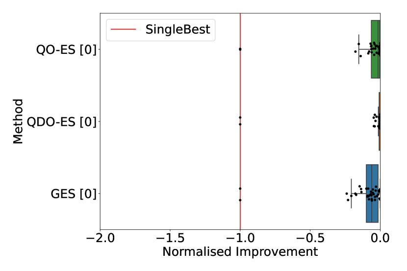
(a) ROC AUC - Binary (41 Datasets)

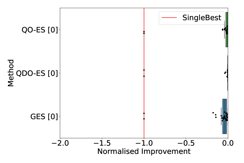
(b) ROC AUC - Multi-class (30 Datasets)

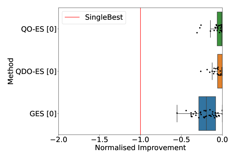
(c) Balanced Accuracy - Binary (41 Datasets)

(d) Balanced Accuracy - Multi-class (30 Datasets)

Figure 4: Normalised Improvement Boxplots for Validation Scores: Higher normalised improvement is better. Each black point represents the improvement for one dataset.

F.3  Ablation Study: Q(D)O-ES Hyperparameter Importance

We perform an ablation study of the components of Q(D)O-ES by determining the importance of hyperparameters on the final performance.

We analyse the importance of hyperparameters using fANOVA (Hutter et al.,, 2014). Therefore, we compute the importance of the hyperparameters defined in Table 3 for each dataset for QO-ES and QDO-ES. Table 4 shows the mean importance (higher is more important) over all datasets split by metric and classification task for QDO-ES and QO-ES.

Table 4: Mean hyperparameter importance computed with fANOVA for QO-ES and QDO-ES (higher means more important).

	QDO-ES				QO-ES
	Balanced Accuracy		ROC AUC		Balanced Accuracy		ROC AUC
Hyperparameter	Binary	Multi-class	Binary	Multi-class	Binary	Multi-class	Binary	Multi-class
Preprocessing	0.57	0.52	0.68	0.51	0.60	0.75	0.69	0.73
Batch Size	0.03	0.03	0.02	0.03	0.03	0.01	0.02	0.02
Archive Size	0.02	0.02	0.01	0.03	0.02	0.01	0.01	0.01
Archive Initialisation	0.15	0.16	0.11	0.21	0.14	0.12	0.10	0.10
Sampling Method	0.15	0.18	0.12	0.16	0.14	0.06	0.11	0.07
Crossover	0.08	0.09	0.06	0.07	0.07	0.06	0.06	0.06

We observe that "Preprocessing", that is, the pruning method before we perform post hoc ensembling, is by far the most important hyperparameter across all scenarios for both QDO-ES and QO-ES. "Archive Initialisation" and "Sampling Method" follow with a similar distance of importance to "Preprocessing" and seem to be important as well. These are followed by "Crossover" with a lower relative importance, while varying "Batch Size" or "Archive Size" do not seem to have any meaningful impact on the final performance.

F.4  Ablation Study: Performance of Hyperparameter Values for Q(D)O-ES

We perform an ablation study of the configurations of the components of Q(D)O-ES by determining the impact of individual hyperparameter values on the final performance.

To assess this performance of individual hyperparameter values, we compute the aggregated normalised improvement per hyperparameter value. That is, we first compute the normalised improvement for all configurations per dataset. Then, we split all configurations based on hyperparameter values and compute the average across all configurations per split; resulting in an average score per dataset for a specific hyperparameter value. Finally, following similar arguments as in Appendix E.3, we compute the median across all datasets per scenario (i.e., the combination of metric and task type). This value now shows the median performance attributed to the hyperparameter value and allows us to interpret how well certain hyperparameter values perform aggregated across datasets. See Table 5 for an overview of the median normalised improvement for all hyperparameters.

Table 5: Median normalised improvement per value of a hyperparameter for QO-ES and QDO-ES (higher is better). A performance of $-1$ is equal to the performance of the SingleBest model, and a performance of $0$ is equal to the performance of the best-observed configuration per dataset.

		QDO-ES				QO-ES
		Balanced Accuracy		ROC AUC		Balanced Accuracy		ROC AUC
Hyperparameter	Value	Binary	Multi-class	Binary	Multi-class	Binary	Multi-class	Binary	Multi-class
Preprocessing	SiloTopN	-0.65	-0.42	-0.27	-0.16	-0.63	-0.46	-0.26	-0.15
	TopN	-0.67	-0.63	-0.33	-0.39	-0.65	-0.63	-0.29	-0.36
Batch Size	20	-0.68	-0.51	-0.3	-0.24	-0.66	-0.49	-0.29	-0.22
	40	-0.67	-0.48	-0.3	-0.25	-0.65	-0.5	-0.31	-0.23
Archive Size	16	-0.66	-0.49	-0.3	-0.24	-0.66	-0.51	-0.3	-0.22
	49	-0.69	-0.5	-0.3	-0.25	-0.65	-0.48	-0.3	-0.22
Archive Initialisation	L1 Ensembles	-0.7	-0.48	-0.3	-0.24	-0.62	-0.46	-0.3	-0.23
	L2 of Single Best	-0.65	-0.51	-0.32	-0.25	-0.65	-0.53	-0.31	-0.23
	Random L2	-0.48	-0.48	-0.24	-0.25	-0.66	-0.48	-0.29	-0.23
Sampling Method	Deterministic	-0.74	-0.54	-0.31	-0.25	-0.68	-0.53	-0.31	-0.24
	Tournament	-0.63	-0.47	-0.3	-0.24	-0.64	-0.48	-0.29	-0.22
	Dynamic	-0.64	-0.48	-0.3	-0.25	-0.62	-0.45	-0.3	-0.22
Crossover	Two-Point	-0.68	-0.47	-0.31	-0.25	-0.65	-0.49	-0.3	-0.22
	Average	-0.64	-0.49	-0.3	-0.24	-0.65	-0.49	-0.28	-0.22
	No	-0.68	-0.53	-0.3	-0.25	-0.67	-0.5	-0.31	-0.23

We observe that the largest difference in performance between hyperparameter values occurs for "Preprocessing"; mirroring the importance of these hyperparameters shown in Table 4. Likewise, the largest difference in performance can be seen for "Preprocessing" in multi-class classification. Likely a result of overfitting, as overfitting is potentially less severe for multi-class classification (Feldman et al.,, 2019).

Appendix G Essential Python Frameworks for the Implementation and Experiments

The following frameworks were essential for our implementation and experiments:

• Auto-Sklearn 1.0 (Feurer et al.,, 2015), Version: 0.14.7, BSD-3-Clause License; We used Auto-Sklearn to generate base models and took the initial code for greedy ensemble selection from Auto-Sklearn’s implementation.

• pyribs (Tjanaka et al.,, 2021), Version 0.4.0, MIT License; We used pyribs’ framework to implement population-based search and the archives.

• Assembled (Purucker and Beel,, 2022), Version 0.0.4, MIT License; We used Assembled to store the base models generated with Auto-Sklearn and to run our ensemble-related experiments.

Appendix H DOIs for Data and Code

The following assets were newly created as part of our experiments:

• The code for our experiments: https://doi.org/10.6084/m9.figshare.23613624.

• The prediction data of base models collected by running Auto-Sklearn 1.0 on the classification datasets from the AutoML benchmark: https://doi.org/10.6084/m9.figshare.23613627.

Appendix I Test and Validation Performance Per Dataset Per Scenario

The following tables provide the exact performance of each ensembling method per dataset. The tables are split per scenario (i.e., the combinations of metric and task type).

Table 6: Test ROC AUC - Binary: The mean and standard deviation of the test score over all folds for each method. The best methods per dataset are shown in bold. All methods close to the best method are considered best (using NumPy’s default $isclose$ function).

Dataset	GES	QDO-ES	QO-ES	SingleBest
APSFailure	0.9917 (± 0.0036)	0.9918 (± 0.0041)	0.9921 (± 0.0036)	0.9912 (± 0.0029)
Amazon_employee_access	0.8681 (± 0.015)	0.8684 (± 0.0134)	0.8684 (± 0.014)	0.8616 (± 0.017)
Australian	0.9317 (± 0.0198)	0.9329 (± 0.0236)	0.9349 (± 0.0202)	0.927 (± 0.0255)
Bioresponse	0.8724 (± 0.0156)	0.8721 (± 0.0169)	0.8731 (± 0.0163)	0.8675 (± 0.0196)
Click_prediction_small	0.7004 (± 0.0142)	0.7009 (± 0.0139)	0.7009 (± 0.0137)	0.6964 (± 0.0152)
Higgs	0.841 (± 0.0017)	0.841 (± 0.0017)	0.841 (± 0.0017)	0.8328 (± 0.002)
Internet-Advertisements	0.987 (± 0.0076)	0.9863 (± 0.0063)	0.9859 (± 0.0077)	0.9759 (± 0.0196)
KDDCup09-Upselling	0.9077 (± 0.009)	0.908 (± 0.0085)	0.9082 (± 0.0085)	0.9058 (± 0.01)
KDDCup09_appetency	0.836 (± 0.0114)	0.8374 (± 0.0126)	0.8385 (± 0.0125)	0.8292 (± 0.0148)
MiniBooNE	0.9874 (± 0.001)	0.9874 (± 0.0011)	0.9874 (± 0.0011)	0.9871 (± 0.001)
PhishingWebsites	0.9968 (± 0.0008)	0.9967 (± 0.001)	0.9966 (± 0.0012)	0.9963 (± 0.0011)
Satellite	0.9836 (± 0.0287)	0.9871 (± 0.019)	0.9886 (± 0.014)	0.9788 (± 0.03)
ada	0.9169 (± 0.019)	0.9172 (± 0.0201)	0.917 (± 0.0199)	0.9155 (± 0.0176)
adult	0.9294 (± 0.0046)	0.9294 (± 0.0045)	0.9294 (± 0.0046)	0.9286 (± 0.0048)
airlines	0.727 (± 0.003)	0.7271 (± 0.0031)	0.7271 (± 0.003)	0.7208 (± 0.0033)
albert	0.7623 (± 0.0026)	0.7623 (± 0.0027)	0.7622 (± 0.0025)	0.7592 (± 0.0038)
arcene	0.8933 (± 0.0981)	0.897 (± 0.0829)	0.8977 (± 0.103)	0.8977 (± 0.1084)
bank-marketing	0.9388 (± 0.0068)	0.9387 (± 0.0067)	0.9388 (± 0.0067)	0.9369 (± 0.0074)
blood-transfusion-service-center	0.7506 (± 0.0459)	0.7467 (± 0.0606)	0.7407 (± 0.0591)	0.7383 (± 0.0386)
christine	0.831 (± 0.0146)	0.8314 (± 0.0144)	0.8317 (± 0.0143)	0.8264 (± 0.0138)
churn	0.9193 (± 0.0266)	0.9212 (± 0.0224)	0.9215 (± 0.0238)	0.9215 (± 0.0245)
credit-g	0.7834 (± 0.0388)	0.7849 (± 0.0374)	0.7863 (± 0.0333)	0.766 (± 0.0383)
gina	0.9936 (± 0.0039)	0.9936 (± 0.004)	0.9937 (± 0.004)	0.9917 (± 0.0049)
guillermo	0.9151 (± 0.0091)	0.9158 (± 0.0087)	0.9157 (± 0.0086)	0.9117 (± 0.0079)
jasmine	0.8825 (± 0.0184)	0.8831 (± 0.019)	0.8824 (± 0.0182)	0.8816 (± 0.0216)
kc1	0.8364 (± 0.0374)	0.8384 (± 0.0355)	0.8388 (± 0.0347)	0.8362 (± 0.0319)
kick	0.7869 (± 0.0077)	0.787 (± 0.0076)	0.7871 (± 0.0076)	0.7808 (± 0.0059)
kr-vs-kp	0.9995 (± 0.0007)	0.9995 (± 0.0008)	0.9994 (± 0.0008)	0.9994 (± 0.0007)
madeline	0.969 (± 0.0061)	0.9689 (± 0.0053)	0.9692 (± 0.0055)	0.9671 (± 0.0051)
nomao	0.9961 (± 0.0009)	0.9961 (± 0.001)	0.9961 (± 0.0009)	0.9959 (± 0.001)
numerai28.6	0.5308 (± 0.0036)	0.5306 (± 0.0037)	0.5306 (± 0.0034)	0.5294 (± 0.0043)
ozone-level-8hr	0.9178 (± 0.0265)	0.9204 (± 0.029)	0.9184 (± 0.0275)	0.912 (± 0.0257)
pc4	0.9448 (± 0.0213)	0.9438 (± 0.0223)	0.9435 (± 0.0203)	0.9331 (± 0.0308)
philippine	0.9149 (± 0.0101)	0.915 (± 0.0103)	0.914 (± 0.0117)	0.9134 (± 0.0114)
phoneme	0.964 (± 0.0069)	0.9643 (± 0.0064)	0.9643 (± 0.0064)	0.9637 (± 0.007)
porto-seguro	0.6401 (± 0.0035)	0.6408 (± 0.0041)	0.6408 (± 0.004)	0.6356 (± 0.0045)
qsar-biodeg	0.928 (± 0.0297)	0.93 (± 0.0294)	0.9288 (± 0.0288)	0.9184 (± 0.0323)
riccardo	0.9997 (± 0.0003)	0.9998 (± 0.0002)	0.9997 (± 0.0002)	0.9997 (± 0.0002)
sf-police-incidents	0.7084 (± 0.0037)	0.7091 (± 0.0033)	0.7092 (± 0.0034)	0.6924 (± 0.0072)
sylvine	0.9927 (± 0.0034)	0.9923 (± 0.0033)	0.9925 (± 0.0033)	0.9915 (± 0.0037)
wilt	0.9953 (± 0.0047)	0.9953 (± 0.0044)	0.9957 (± 0.0034)	0.9949 (± 0.0045)

Table 7: Test ROC AUC - Multi-class: The mean and standard deviation of the test score over all folds for each method. The best methods per dataset are shown in bold. All methods close to the best method are considered best (using NumPy’s default $isclose$ function).

Dataset	GES	QDO-ES	QO-ES	SingleBest
Diabetes130US	0.7143 (± 0.0064)	0.7142 (± 0.0064)	0.7144 (± 0.0067)	0.7099 (± 0.0051)
Fashion-MNIST	0.9945 (± 0.0005)	0.9946 (± 0.0005)	0.9945 (± 0.0005)	0.9942 (± 0.0005)
GesturePhaseSegmentationProcessed	0.9137 (± 0.0086)	0.9137 (± 0.0083)	0.9143 (± 0.0085)	0.9039 (± 0.0055)
KDDCup99	0.9987 (± 0.0042)	0.9992 (± 0.0018)	0.9991 (± 0.0018)	0.9997 (± 0.0007)
amazon-commerce-reviews	0.9946 (± 0.0032)	0.9945 (± 0.0034)	0.9948 (± 0.0029)	0.9859 (± 0.0052)
car	0.9998 (± 0.0006)	1.0 (± 0.0001)	1.0 (± 0.0001)	1.0 (± 0.0001)
cmc	0.7475 (± 0.0329)	0.7468 (± 0.0315)	0.7477 (± 0.0328)	0.7391 (± 0.0298)
cnae-9	0.9977 (± 0.0019)	0.9978 (± 0.0015)	0.998 (± 0.0011)	0.9952 (± 0.0037)
connect-4	0.9405 (± 0.0039)	0.9408 (± 0.0038)	0.9408 (± 0.0039)	0.9371 (± 0.0026)
covertype	0.9991 (± 0.0001)	0.9991 (± 0.0001)	0.9991 (± 0.0001)	0.9988 (± 0.0001)
dilbert	0.9999 (± 0.0001)	0.9999 (± 0.0)	0.9999 (± 0.0)	0.9998 (± 0.0001)
dionis	0.9993 (± 0.0001)	0.9993 (± 0.0001)	0.9993 (± 0.0001)	0.9987 (± 0.0003)
dna	0.9947 (± 0.0033)	0.995 (± 0.0032)	0.995 (± 0.0032)	0.9941 (± 0.0036)
eucalyptus	0.9222 (± 0.016)	0.9205 (± 0.017)	0.9212 (± 0.0148)	0.9162 (± 0.0172)
fabert	0.9428 (± 0.0034)	0.9428 (± 0.0033)	0.9427 (± 0.0033)	0.9334 (± 0.0044)
first-order-theorem-proving	0.8398 (± 0.0118)	0.8398 (± 0.0113)	0.84 (± 0.0112)	0.8359 (± 0.0127)
helena	0.8917 (± 0.0025)	0.8919 (± 0.0025)	0.8919 (± 0.0025)	0.8778 (± 0.0029)
jannis	0.8853 (± 0.0034)	0.8856 (± 0.0034)	0.8856 (± 0.0033)	0.8802 (± 0.0035)
jungle_chess_2pcs_raw_endgame_complete	0.9927 (± 0.0017)	0.9926 (± 0.0016)	0.9927 (± 0.0016)	0.9915 (± 0.0022)
mfeat-factors	0.9983 (± 0.0028)	0.9985 (± 0.0028)	0.9984 (± 0.0026)	0.9988 (± 0.0009)
micro-mass	0.9966 (± 0.0031)	0.9965 (± 0.0032)	0.9978 (± 0.0018)	0.9939 (± 0.0084)
okcupid-stem	0.8288 (± 0.0056)	0.829 (± 0.0055)	0.8289 (± 0.0054)	0.8258 (± 0.0054)
robert	0.8982 (± 0.0048)	0.8984 (± 0.0042)	0.8987 (± 0.0045)	0.8864 (± 0.0066)
segment	0.9956 (± 0.0017)	0.9953 (± 0.0019)	0.9958 (± 0.0016)	0.9949 (± 0.0021)
shuttle	0.9928 (± 0.0226)	1.0 (± 0.0)	1.0 (± 0.0)	1.0 (± 0.0)
steel-plates-fault	0.9618 (± 0.0074)	0.9629 (± 0.0067)	0.9621 (± 0.0078)	0.9569 (± 0.0119)
vehicle	0.9679 (± 0.0088)	0.9671 (± 0.0102)	0.9682 (± 0.0092)	0.9656 (± 0.0089)
volkert	0.9565 (± 0.0023)	0.957 (± 0.0018)	0.9567 (± 0.0021)	0.9531 (± 0.0022)
wine-quality-white	0.866 (± 0.0329)	0.864 (± 0.0284)	0.8652 (± 0.0331)	0.8613 (± 0.0394)
yeast	0.8771 (± 0.0386)	0.8743 (± 0.0445)	0.877 (± 0.0371)	0.8627 (± 0.0365)

Table 8: Test Balanced Accuracy - Binary: The mean and standard deviation of the test score over all folds for each method. The best methods per dataset are shown in bold. All methods close to the best method are considered best (using NumPy’s default $isclose$ function).

Dataset	GES	QDO-ES	QO-ES	SingleBest
APSFailure	0.9625 (± 0.0073)	0.9608 (± 0.0105)	0.9594 (± 0.0082)	0.9539 (± 0.0128)
Amazon_employee_access	0.7914 (± 0.0089)	0.7913 (± 0.0112)	0.7923 (± 0.0121)	0.7837 (± 0.0142)
Australian	0.8526 (± 0.0331)	0.8582 (± 0.0285)	0.8612 (± 0.0307)	0.8471 (± 0.0287)
Bioresponse	0.7911 (± 0.0151)	0.7924 (± 0.0125)	0.7956 (± 0.0171)	0.7946 (± 0.0181)
Click_prediction_small	0.6365 (± 0.0142)	0.6381 (± 0.0119)	0.6384 (± 0.0129)	0.6377 (± 0.0146)
Higgs	0.7518 (± 0.0016)	0.7519 (± 0.0017)	0.752 (± 0.0016)	0.7469 (± 0.0027)
Internet-Advertisements	0.9445 (± 0.0203)	0.9481 (± 0.0215)	0.9455 (± 0.024)	0.9442 (± 0.0225)
KDDCup09-Upselling	0.7985 (± 0.0104)	0.7993 (± 0.0125)	0.8002 (± 0.0099)	0.8001 (± 0.0105)
KDDCup09_appetency	0.7492 (± 0.0134)	0.7472 (± 0.022)	0.7505 (± 0.0163)	0.7465 (± 0.0168)
MiniBooNE	0.9462 (± 0.003)	0.9461 (± 0.0032)	0.9464 (± 0.0032)	0.9443 (± 0.0026)
PhishingWebsites	0.9706 (± 0.0049)	0.9695 (± 0.0038)	0.9696 (± 0.0051)	0.9696 (± 0.0037)
Satellite	0.8738 (± 0.0728)	0.8936 (± 0.0832)	0.8613 (± 0.0597)	0.925 (± 0.093)
ada	0.8324 (± 0.0322)	0.8352 (± 0.0289)	0.8339 (± 0.0277)	0.8316 (± 0.0304)
adult	0.843 (± 0.0073)	0.8431 (± 0.0079)	0.8439 (± 0.0079)	0.8428 (± 0.0083)
airlines	0.6624 (± 0.0025)	0.6628 (± 0.0022)	0.6628 (± 0.0025)	0.6583 (± 0.0022)
albert	0.6917 (± 0.0036)	0.6917 (± 0.0037)	0.6918 (± 0.0037)	0.6892 (± 0.0027)
arcene	0.8208 (± 0.1933)	0.7792 (± 0.1827)	0.7917 (± 0.1784)	0.7525 (± 0.2149)
bank-marketing	0.874 (± 0.0108)	0.8739 (± 0.0099)	0.8746 (± 0.0107)	0.8736 (± 0.0098)
blood-transfusion-service-center	0.67 (± 0.0409)	0.6821 (± 0.0483)	0.6746 (± 0.051)	0.6816 (± 0.055)
christine	0.754 (± 0.015)	0.7575 (± 0.0156)	0.7553 (± 0.0174)	0.7482 (± 0.0204)
churn	0.9094 (± 0.0143)	0.9112 (± 0.0191)	0.912 (± 0.0156)	0.9087 (± 0.0161)
credit-g	0.6983 (± 0.0563)	0.7079 (± 0.0592)	0.7145 (± 0.035)	0.6936 (± 0.0353)
gina	0.9663 (± 0.0106)	0.9625 (± 0.0157)	0.9628 (± 0.0141)	0.9622 (± 0.0149)
guillermo	0.8366 (± 0.0119)	0.835 (± 0.0115)	0.8377 (± 0.0117)	0.8341 (± 0.0112)
jasmine	0.8173 (± 0.0205)	0.8163 (± 0.0169)	0.8197 (± 0.0189)	0.8123 (± 0.0226)
kc1	0.7363 (± 0.0316)	0.7543 (± 0.0285)	0.7512 (± 0.0345)	0.7344 (± 0.0285)
kick	0.7003 (± 0.0081)	0.6993 (± 0.0082)	0.7024 (± 0.0079)	0.698 (± 0.0059)
kr-vs-kp	0.9943 (± 0.0052)	0.9933 (± 0.0059)	0.9943 (± 0.0052)	0.993 (± 0.0062)
madeline	0.9108 (± 0.0117)	0.9073 (± 0.0133)	0.9169 (± 0.0107)	0.9083 (± 0.0171)
nomao	0.9688 (± 0.0029)	0.9684 (± 0.0026)	0.9691 (± 0.0024)	0.9682 (± 0.0021)
numerai28.6	0.5204 (± 0.0046)	0.5204 (± 0.0049)	0.5215 (± 0.0043)	0.5189 (± 0.0047)
ozone-level-8hr	0.8234 (± 0.0353)	0.8259 (± 0.0383)	0.8296 (± 0.037)	0.8337 (± 0.0305)
pc4	0.8763 (± 0.0365)	0.8791 (± 0.051)	0.883 (± 0.0392)	0.8719 (± 0.0406)
philippine	0.8368 (± 0.0108)	0.8332 (± 0.0124)	0.8342 (± 0.0135)	0.8296 (± 0.0158)
phoneme	0.8902 (± 0.0176)	0.8914 (± 0.0134)	0.8886 (± 0.015)	0.8893 (± 0.0136)
porto-seguro	0.5991 (± 0.0056)	0.5991 (± 0.0041)	0.6 (± 0.0047)	0.5989 (± 0.0054)
qsar-biodeg	0.8539 (± 0.039)	0.8537 (± 0.0303)	0.8538 (± 0.041)	0.8403 (± 0.0271)
riccardo	0.998 (± 0.0007)	0.9983 (± 0.0007)	0.9978 (± 0.0007)	0.9981 (± 0.0007)
sf-police-incidents	0.6375 (± 0.0043)	0.6377 (± 0.0032)	0.6373 (± 0.0041)	0.6257 (± 0.0048)
sylvine	0.9567 (± 0.0079)	0.9567 (± 0.0068)	0.9567 (± 0.0063)	0.9561 (± 0.0082)
wilt	0.9676 (± 0.0165)	0.9644 (± 0.0186)	0.9622 (± 0.0199)	0.9771 (± 0.0136)

Table 9: Test Balanced Accuracy - Multi-class: The mean and standard deviation of the test score over all folds for each method. The best methods per dataset are shown in bold. All methods close to the best method are considered best (using NumPy’s default $isclose$ function).

Dataset	GES	QDO-ES	QO-ES	SingleBest
Diabetes130US	0.4996 (± 0.0071)	0.4993 (± 0.0065)	0.4994 (± 0.005)	0.4964 (± 0.0058)
Fashion-MNIST	0.9124 (± 0.0042)	0.9129 (± 0.0042)	0.9121 (± 0.0038)	0.9046 (± 0.0062)
GesturePhaseSegmentationProcessed	0.6749 (± 0.0209)	0.6766 (± 0.0194)	0.6771 (± 0.0232)	0.641 (± 0.0137)
KDDCup99	0.8113 (± 0.0638)	0.8076 (± 0.0677)	0.8071 (± 0.06)	0.7985 (± 0.0547)
amazon-commerce-reviews	0.868 (± 0.0279)	0.866 (± 0.0284)	0.862 (± 0.031)	0.8153 (± 0.0327)
car	0.9932 (± 0.0111)	0.9917 (± 0.0113)	0.9913 (± 0.0125)	0.9932 (± 0.0066)
cmc	0.5499 (± 0.0441)	0.5513 (± 0.0408)	0.5532 (± 0.0328)	0.5482 (± 0.0368)
cnae-9	0.9509 (± 0.0164)	0.9509 (± 0.0152)	0.9528 (± 0.0172)	0.9454 (± 0.0177)
connect-4	0.7634 (± 0.009)	0.7632 (± 0.0078)	0.7615 (± 0.0081)	0.7594 (± 0.0085)
covertype	0.9633 (± 0.0026)	0.9635 (± 0.003)	0.9635 (± 0.0027)	0.956 (± 0.0031)
dilbert	0.9949 (± 0.0021)	0.9945 (± 0.003)	0.9943 (± 0.0025)	0.9943 (± 0.0027)
dionis	0.8462 (± 0.017)	0.8485 (± 0.0163)	0.8475 (± 0.0164)	0.841 (± 0.0107)
dna	0.9619 (± 0.0119)	0.9655 (± 0.0124)	0.9654 (± 0.0117)	0.959 (± 0.0116)
eucalyptus	0.6463 (± 0.0705)	0.6426 (± 0.0658)	0.62 (± 0.0526)	0.6264 (± 0.0538)
fabert	0.7115 (± 0.0117)	0.7148 (± 0.0104)	0.7141 (± 0.0104)	0.6952 (± 0.0146)
first-order-theorem-proving	0.5116 (± 0.0223)	0.5107 (± 0.0238)	0.5069 (± 0.0188)	0.5028 (± 0.0203)
helena	0.2743 (± 0.0066)	0.2783 (± 0.005)	0.2775 (± 0.0065)	0.2644 (± 0.0052)
jannis	0.6504 (± 0.0106)	0.6506 (± 0.0109)	0.6504 (± 0.0107)	0.6484 (± 0.0085)
jungle_chess_2pcs_raw_endgame_complete	0.9261 (± 0.0116)	0.9268 (± 0.011)	0.925 (± 0.0132)	0.9182 (± 0.0139)
mfeat-factors	0.982 (± 0.0075)	0.982 (± 0.0063)	0.981 (± 0.0077)	0.981 (± 0.0077)
micro-mass	0.9137 (± 0.0341)	0.906 (± 0.0426)	0.9088 (± 0.0536)	0.9108 (± 0.0361)
okcupid-stem	0.6971 (± 0.0083)	0.6961 (± 0.0088)	0.6969 (± 0.0077)	0.6956 (± 0.0091)
robert	0.5327 (± 0.0115)	0.5384 (± 0.0125)	0.5371 (± 0.0134)	0.5258 (± 0.0106)
segment	0.9346 (± 0.0183)	0.9342 (± 0.0201)	0.9368 (± 0.0179)	0.929 (± 0.0218)
shuttle	0.9534 (± 0.0674)	0.9677 (± 0.0594)	0.9685 (± 0.0594)	0.9677 (± 0.0594)
steel-plates-fault	0.831 (± 0.0254)	0.8331 (± 0.0234)	0.8367 (± 0.0208)	0.8138 (± 0.033)
vehicle	0.8447 (± 0.0332)	0.8343 (± 0.0321)	0.8366 (± 0.0266)	0.8352 (± 0.0398)
volkert	0.7087 (± 0.0107)	0.7085 (± 0.008)	0.7114 (± 0.0079)	0.6699 (± 0.0073)
wine-quality-white	0.4546 (± 0.0463)	0.4345 (± 0.0405)	0.4469 (± 0.0457)	0.4271 (± 0.0678)
yeast	0.5786 (± 0.0705)	0.5728 (± 0.0664)	0.5657 (± 0.0579)	0.5631 (± 0.0772)

Table 10: Validation ROC AUC - Binary: The mean and standard deviation of the validation score over all folds for each method. The best methods per dataset are shown in bold. All methods close to the best method are considered best (using NumPy’s default $isclose$ function).

Dataset	GES	QDO-ES	QO-ES	SingleBest
APSFailure	0.9952 (± 0.001)	0.9953 (± 0.001)	0.9952 (± 0.0009)	0.9943 (± 0.001)
Amazon_employee_access	0.8703 (± 0.0072)	0.8712 (± 0.0076)	0.8705 (± 0.0075)	0.8596 (± 0.0067)
Australian	0.9604 (± 0.0109)	0.9611 (± 0.0105)	0.961 (± 0.0107)	0.9525 (± 0.0122)
Bioresponse	0.8768 (± 0.0084)	0.8772 (± 0.0078)	0.8771 (± 0.0079)	0.8701 (± 0.0083)
Click_prediction_small	0.7042 (± 0.0047)	0.7043 (± 0.0047)	0.7042 (± 0.0046)	0.6999 (± 0.0051)
Higgs	0.8406 (± 0.002)	0.8406 (± 0.002)	0.8407 (± 0.0021)	0.8325 (± 0.002)
Internet-Advertisements	0.9935 (± 0.003)	0.9941 (± 0.0019)	0.994 (± 0.0019)	0.9898 (± 0.0029)
KDDCup09-Upselling	0.9124 (± 0.0033)	0.9131 (± 0.0031)	0.9129 (± 0.003)	0.9092 (± 0.0028)
KDDCup09_appetency	0.8429 (± 0.0106)	0.8432 (± 0.0105)	0.8431 (± 0.0106)	0.8325 (± 0.0106)
MiniBooNE	0.9875 (± 0.0004)	0.9874 (± 0.0004)	0.9874 (± 0.0005)	0.987 (± 0.0005)
PhishingWebsites	0.9971 (± 0.0003)	0.9971 (± 0.0003)	0.9971 (± 0.0003)	0.9968 (± 0.0004)
Satellite	0.9989 (± 0.0012)	0.9991 (± 0.0011)	0.999 (± 0.0013)	0.9984 (± 0.0013)
ada	0.9235 (± 0.0049)	0.9239 (± 0.0048)	0.9236 (± 0.0048)	0.9202 (± 0.0058)
adult	0.9301 (± 0.0018)	0.9301 (± 0.0018)	0.9301 (± 0.0018)	0.9293 (± 0.0018)
airlines	0.7271 (± 0.0015)	0.7272 (± 0.0016)	0.7272 (± 0.0015)	0.721 (± 0.0019)
albert	0.7621 (± 0.0021)	0.7621 (± 0.0021)	0.7621 (± 0.0021)	0.7588 (± 0.0035)
arcene	0.9977 (± 0.0049)	0.9986 (± 0.0043)	0.9986 (± 0.0043)	0.9749 (± 0.0252)
bank-marketing	0.9386 (± 0.0024)	0.9387 (± 0.0024)	0.9387 (± 0.0024)	0.937 (± 0.0033)
blood-transfusion-service-center	0.7759 (± 0.0098)	0.7787 (± 0.0117)	0.7771 (± 0.0127)	0.7598 (± 0.0134)
christine	0.8449 (± 0.0079)	0.845 (± 0.0078)	0.8449 (± 0.0079)	0.835 (± 0.0069)
churn	0.9448 (± 0.0128)	0.9446 (± 0.0128)	0.9448 (± 0.0127)	0.9405 (± 0.0134)
credit-g	0.8371 (± 0.0231)	0.8389 (± 0.022)	0.8379 (± 0.0225)	0.8188 (± 0.0234)
gina	0.9956 (± 0.0015)	0.9956 (± 0.0015)	0.9956 (± 0.0015)	0.9949 (± 0.0021)
guillermo	0.9162 (± 0.0028)	0.9168 (± 0.0026)	0.9169 (± 0.0027)	0.9129 (± 0.0017)
jasmine	0.8974 (± 0.012)	0.8978 (± 0.0122)	0.8979 (± 0.0121)	0.8882 (± 0.0135)
kc1	0.8598 (± 0.0098)	0.8595 (± 0.0095)	0.8594 (± 0.0092)	0.8496 (± 0.0103)
kick	0.7923 (± 0.0049)	0.7924 (± 0.005)	0.7923 (± 0.005)	0.7842 (± 0.0038)
kr-vs-kp	0.9999 (± 0.0002)	0.9999 (± 0.0001)	0.9999 (± 0.0001)	0.9998 (± 0.0002)
madeline	0.9718 (± 0.0034)	0.9721 (± 0.0033)	0.9719 (± 0.0033)	0.9681 (± 0.0034)
nomao	0.9964 (± 0.0002)	0.9964 (± 0.0002)	0.9964 (± 0.0002)	0.9962 (± 0.0002)
numerai28.6	0.5344 (± 0.0025)	0.5346 (± 0.0026)	0.5347 (± 0.0026)	0.5312 (± 0.0027)
ozone-level-8hr	0.9554 (± 0.0093)	0.9571 (± 0.0079)	0.956 (± 0.0091)	0.9486 (± 0.0078)
pc4	0.9677 (± 0.0081)	0.9677 (± 0.0075)	0.9676 (± 0.0075)	0.9543 (± 0.0107)
philippine	0.9202 (± 0.0076)	0.9205 (± 0.0075)	0.9205 (± 0.0075)	0.918 (± 0.0074)
phoneme	0.9636 (± 0.0041)	0.964 (± 0.0035)	0.9641 (± 0.0033)	0.962 (± 0.0043)
porto-seguro	0.6429 (± 0.0017)	0.6432 (± 0.002)	0.6432 (± 0.002)	0.6371 (± 0.0037)
qsar-biodeg	0.9554 (± 0.0057)	0.9559 (± 0.0064)	0.9559 (± 0.0062)	0.9449 (± 0.0081)
riccardo	0.9999 (± 0.0)	0.9999 (± 0.0)	0.9999 (± 0.0001)	0.9999 (± 0.0)
sf-police-incidents	0.708 (± 0.0036)	0.7085 (± 0.0033)	0.7085 (± 0.0034)	0.6923 (± 0.007)
sylvine	0.9928 (± 0.0013)	0.9928 (± 0.0013)	0.9927 (± 0.0014)	0.9922 (± 0.0016)
wilt	0.9982 (± 0.0013)	0.9982 (± 0.0012)	0.9982 (± 0.0013)	0.9976 (± 0.0017)

Table 11: Validation ROC AUC - Multi-class: The mean and standard deviation of the validation score over all folds for each method. The best methods per dataset are shown in bold. All methods close to the best method are considered best (using NumPy’s default $isclose$ function).

Dataset	GES	QDO-ES	QO-ES	SingleBest
Diabetes130US	0.7146 (± 0.0038)	0.7147 (± 0.0038)	0.7147 (± 0.0038)	0.7101 (± 0.0024)
Fashion-MNIST	0.9946 (± 0.0004)	0.9946 (± 0.0004)	0.9946 (± 0.0004)	0.9942 (± 0.0004)
GesturePhaseSegmentationProcessed	0.9152 (± 0.0064)	0.9153 (± 0.0064)	0.9154 (± 0.0064)	0.9056 (± 0.0039)
KDDCup99	0.9999 (± 0.0001)	0.9999 (± 0.0001)	0.9999 (± 0.0001)	0.9995 (± 0.0006)
amazon-commerce-reviews	0.9959 (± 0.001)	0.996 (± 0.001)	0.9959 (± 0.001)	0.9878 (± 0.0032)
car	1.0 (± 0.0)	1.0 (± 0.0)	1.0 (± 0.0)	1.0 (± 0.0)
cmc	0.7804 (± 0.0191)	0.7804 (± 0.0193)	0.7802 (± 0.0195)	0.7665 (± 0.0197)
cnae-9	0.9992 (± 0.0003)	0.9992 (± 0.0003)	0.9992 (± 0.0003)	0.9985 (± 0.0006)
connect-4	0.9423 (± 0.0017)	0.9426 (± 0.0017)	0.9425 (± 0.0017)	0.9393 (± 0.0018)
covertype	0.9991 (± 0.0001)	0.9991 (± 0.0001)	0.9991 (± 0.0001)	0.9989 (± 0.0001)
dilbert	1.0 (± 0.0)	1.0 (± 0.0)	1.0 (± 0.0)	0.9999 (± 0.0)
dionis	0.9993 (± 0.0001)	0.9993 (± 0.0001)	0.9993 (± 0.0001)	0.9987 (± 0.0003)
dna	0.9962 (± 0.0009)	0.9964 (± 0.0009)	0.9963 (± 0.0009)	0.9954 (± 0.001)
eucalyptus	0.9382 (± 0.0056)	0.9386 (± 0.0054)	0.9384 (± 0.0057)	0.928 (± 0.0056)
fabert	0.9448 (± 0.0018)	0.945 (± 0.0017)	0.945 (± 0.0017)	0.9355 (± 0.0024)
first-order-theorem-proving	0.8444 (± 0.0027)	0.8449 (± 0.0025)	0.8449 (± 0.0024)	0.8369 (± 0.0035)
helena	0.8933 (± 0.0023)	0.8935 (± 0.0021)	0.8935 (± 0.0021)	0.8792 (± 0.0025)
jannis	0.8838 (± 0.0023)	0.884 (± 0.0024)	0.8839 (± 0.0025)	0.8781 (± 0.003)
jungle_chess_2pcs_raw_endgame_complete	0.993 (± 0.0015)	0.993 (± 0.0015)	0.993 (± 0.0015)	0.9918 (± 0.002)
mfeat-factors	0.9998 (± 0.0002)	0.9998 (± 0.0002)	0.9998 (± 0.0002)	0.9996 (± 0.0004)
micro-mass	0.9995 (± 0.0005)	0.9995 (± 0.0005)	0.9995 (± 0.0004)	0.9991 (± 0.0007)
okcupid-stem	0.8287 (± 0.0021)	0.8289 (± 0.0022)	0.8289 (± 0.0022)	0.8259 (± 0.0018)
robert	0.9009 (± 0.0035)	0.9011 (± 0.0034)	0.9011 (± 0.0035)	0.8903 (± 0.0032)
segment	0.9975 (± 0.0007)	0.9975 (± 0.0008)	0.9975 (± 0.0008)	0.9967 (± 0.001)
shuttle	1.0 (± 0.0)	1.0 (± 0.0)	1.0 (± 0.0)	1.0 (± 0.0)
steel-plates-fault	0.9712 (± 0.0047)	0.9716 (± 0.0044)	0.9715 (± 0.0045)	0.9688 (± 0.0041)
vehicle	0.9779 (± 0.0044)	0.9779 (± 0.0044)	0.9778 (± 0.0043)	0.9734 (± 0.0047)
volkert	0.9572 (± 0.0019)	0.9573 (± 0.0017)	0.9572 (± 0.0019)	0.9536 (± 0.0018)
wine-quality-white	0.9064 (± 0.0075)	0.9068 (± 0.0078)	0.9064 (± 0.0077)	0.8982 (± 0.0072)
yeast	0.8947 (± 0.0125)	0.8961 (± 0.0137)	0.8956 (± 0.0134)	0.8795 (± 0.0142)

Table 12: Validation Balanced Accuracy - Binary: The mean and standard deviation of the validation score over all folds for each method. The best methods per dataset are shown in bold. All methods close to the best method are considered best (using NumPy’s default $isclose$ function).

Dataset	GES	QDO-ES	QO-ES	SingleBest
APSFailure	0.9718 (± 0.0033)	0.9723 (± 0.0035)	0.9727 (± 0.0036)	0.9663 (± 0.0048)
Amazon_employee_access	0.8 (± 0.0071)	0.8041 (± 0.0077)	0.804 (± 0.0074)	0.7863 (± 0.0092)
Australian	0.9113 (± 0.0106)	0.9192 (± 0.0105)	0.9178 (± 0.0092)	0.9049 (± 0.0127)
Bioresponse	0.8079 (± 0.0126)	0.8129 (± 0.0107)	0.8137 (± 0.01)	0.7984 (± 0.0111)
Click_prediction_small	0.6485 (± 0.0039)	0.6489 (± 0.0048)	0.6492 (± 0.0043)	0.6444 (± 0.0047)
Higgs	0.7518 (± 0.0015)	0.752 (± 0.0017)	0.752 (± 0.0017)	0.7464 (± 0.0028)
Internet-Advertisements	0.9664 (± 0.0052)	0.9689 (± 0.005)	0.9688 (± 0.0068)	0.9618 (± 0.0058)
KDDCup09-Upselling	0.8112 (± 0.0057)	0.8128 (± 0.0062)	0.8123 (± 0.0059)	0.8052 (± 0.0054)
KDDCup09_appetency	0.7749 (± 0.0157)	0.7744 (± 0.0152)	0.7744 (± 0.0162)	0.7636 (± 0.013)
MiniBooNE	0.9475 (± 0.0014)	0.9477 (± 0.0013)	0.9478 (± 0.0013)	0.9449 (± 0.0016)
PhishingWebsites	0.9754 (± 0.0019)	0.9756 (± 0.0019)	0.9764 (± 0.0018)	0.9733 (± 0.0018)
Satellite	0.9916 (± 0.0114)	0.9924 (± 0.0123)	0.9922 (± 0.0117)	0.9844 (± 0.0182)
ada	0.8535 (± 0.0083)	0.8554 (± 0.0086)	0.8549 (± 0.0083)	0.846 (± 0.0091)
adult	0.8474 (± 0.0031)	0.8472 (± 0.003)	0.8474 (± 0.0029)	0.8453 (± 0.0029)
airlines	0.6634 (± 0.001)	0.6636 (± 0.001)	0.6638 (± 0.001)	0.658 (± 0.0012)
albert	0.6931 (± 0.0018)	0.6932 (± 0.0022)	0.6933 (± 0.0021)	0.6897 (± 0.0017)
arcene	0.9602 (± 0.0326)	0.9699 (± 0.0227)	0.969 (± 0.0241)	0.9437 (± 0.0339)
bank-marketing	0.8781 (± 0.0044)	0.8779 (± 0.0046)	0.8782 (± 0.0044)	0.8765 (± 0.0042)
blood-transfusion-service-center	0.73 (± 0.0227)	0.7354 (± 0.0206)	0.7282 (± 0.0192)	0.7078 (± 0.0168)
christine	0.7794 (± 0.0063)	0.784 (± 0.0071)	0.7825 (± 0.0071)	0.7666 (± 0.0059)
churn	0.9193 (± 0.0108)	0.9204 (± 0.0102)	0.9206 (± 0.01)	0.9144 (± 0.0103)
credit-g	0.7727 (± 0.0204)	0.7799 (± 0.0213)	0.7779 (± 0.0209)	0.7571 (± 0.0219)
gina	0.9775 (± 0.0038)	0.9773 (± 0.0037)	0.9775 (± 0.0033)	0.9733 (± 0.0055)
guillermo	0.8421 (± 0.003)	0.8441 (± 0.002)	0.844 (± 0.0028)	0.8364 (± 0.0018)
jasmine	0.8415 (± 0.0103)	0.842 (± 0.0105)	0.8412 (± 0.0103)	0.8273 (± 0.0079)
kc1	0.7852 (± 0.0153)	0.7926 (± 0.0137)	0.7893 (± 0.0096)	0.7696 (± 0.0152)
kick	0.7094 (± 0.0034)	0.7092 (± 0.004)	0.71 (± 0.0039)	0.7033 (± 0.0038)
kr-vs-kp	0.998 (± 0.0018)	0.9982 (± 0.0013)	0.9982 (± 0.0015)	0.9975 (± 0.0023)
madeline	0.928 (± 0.0066)	0.9294 (± 0.0057)	0.929 (± 0.0063)	0.9207 (± 0.0086)
nomao	0.9727 (± 0.0016)	0.9726 (± 0.0017)	0.9728 (± 0.0016)	0.9711 (± 0.0013)
numerai28.6	0.5268 (± 0.003)	0.527 (± 0.0023)	0.5272 (± 0.0028)	0.5234 (± 0.0025)
ozone-level-8hr	0.9079 (± 0.0154)	0.9139 (± 0.0089)	0.9102 (± 0.0155)	0.9004 (± 0.0136)
pc4	0.9203 (± 0.015)	0.9285 (± 0.01)	0.9281 (± 0.0117)	0.9071 (± 0.0119)
philippine	0.8479 (± 0.0103)	0.8488 (± 0.0098)	0.8494 (± 0.0093)	0.8395 (± 0.0103)
phoneme	0.9019 (± 0.004)	0.9042 (± 0.0039)	0.9035 (± 0.0036)	0.8927 (± 0.0039)
porto-seguro	0.6041 (± 0.0021)	0.6037 (± 0.0019)	0.6043 (± 0.0022)	0.6006 (± 0.0022)
qsar-biodeg	0.9108 (± 0.011)	0.9157 (± 0.009)	0.9143 (± 0.0101)	0.8933 (± 0.0133)
riccardo	0.999 (± 0.0004)	0.999 (± 0.0004)	0.999 (± 0.0004)	0.9987 (± 0.0005)
sf-police-incidents	0.6376 (± 0.0038)	0.6387 (± 0.0037)	0.6377 (± 0.0039)	0.6252 (± 0.0055)
sylvine	0.965 (± 0.0037)	0.9654 (± 0.0028)	0.9657 (± 0.0034)	0.963 (± 0.0038)
wilt	0.9891 (± 0.0054)	0.9907 (± 0.0055)	0.9894 (± 0.0056)	0.9866 (± 0.0052)

Table 13: Validation Balanced Accuracy - Multi-class: The mean and standard deviation of the validation score over all folds for each method. The best methods per dataset are shown in bold. All methods close to the best method are considered best (using NumPy’s default $isclose$ function).

Dataset	GES	QDO-ES	QO-ES	SingleBest
Diabetes130US	0.5045 (± 0.0019)	0.5041 (± 0.0021)	0.5042 (± 0.0017)	0.5002 (± 0.0022)
Fashion-MNIST	0.9141 (± 0.0029)	0.9154 (± 0.003)	0.915 (± 0.0027)	0.9049 (± 0.0048)
GesturePhaseSegmentationProcessed	0.6966 (± 0.0186)	0.6971 (± 0.0187)	0.6971 (± 0.0197)	0.6565 (± 0.0107)
KDDCup99	0.7938 (± 0.02)	0.8072 (± 0.0223)	0.8026 (± 0.0208)	0.7841 (± 0.0195)
amazon-commerce-reviews	0.8868 (± 0.0166)	0.8942 (± 0.0152)	0.8921 (± 0.0176)	0.8337 (± 0.0159)
car	0.9983 (± 0.0039)	0.9994 (± 0.0017)	0.9992 (± 0.0017)	0.9969 (± 0.0066)
cmc	0.6256 (± 0.0167)	0.6326 (± 0.0162)	0.6291 (± 0.015)	0.6087 (± 0.0165)
cnae-9	0.9773 (± 0.0083)	0.9782 (± 0.0079)	0.9782 (± 0.0076)	0.9711 (± 0.0085)
connect-4	0.7727 (± 0.0068)	0.7733 (± 0.0066)	0.7731 (± 0.0064)	0.7683 (± 0.0062)
covertype	0.9641 (± 0.0016)	0.9647 (± 0.0017)	0.9644 (± 0.0014)	0.9553 (± 0.0011)
dilbert	0.9973 (± 0.0008)	0.9975 (± 0.0007)	0.9974 (± 0.0008)	0.9953 (± 0.0019)
dionis	0.8463 (± 0.0172)	0.8487 (± 0.0159)	0.8476 (± 0.0164)	0.8406 (± 0.0108)
dna	0.9735 (± 0.0051)	0.9763 (± 0.0035)	0.9749 (± 0.0047)	0.9708 (± 0.0052)
eucalyptus	0.7454 (± 0.0168)	0.7467 (± 0.0083)	0.7484 (± 0.0159)	0.7172 (± 0.0098)
fabert	0.7306 (± 0.0047)	0.7353 (± 0.0054)	0.7353 (± 0.0062)	0.71 (± 0.01)
first-order-theorem-proving	0.5311 (± 0.008)	0.5342 (± 0.0078)	0.5339 (± 0.0081)	0.5178 (± 0.0071)
helena	0.2777 (± 0.006)	0.2819 (± 0.0066)	0.2812 (± 0.0073)	0.2659 (± 0.0047)
jannis	0.654 (± 0.0068)	0.6549 (± 0.0063)	0.6545 (± 0.0066)	0.648 (± 0.0058)
jungle_chess_2pcs_raw_endgame_complete	0.9307 (± 0.0121)	0.9314 (± 0.0124)	0.9311 (± 0.0123)	0.923 (± 0.0115)
mfeat-factors	0.9934 (± 0.0033)	0.9934 (± 0.0035)	0.9936 (± 0.0035)	0.9914 (± 0.0038)
micro-mass	0.967 (± 0.0147)	0.9665 (± 0.0159)	0.9659 (± 0.0162)	0.9604 (± 0.0179)
okcupid-stem	0.7027 (± 0.003)	0.7032 (± 0.0024)	0.7033 (± 0.0026)	0.6994 (± 0.0023)
robert	0.5527 (± 0.0091)	0.5564 (± 0.0099)	0.5554 (± 0.0104)	0.5347 (± 0.0112)
segment	0.9596 (± 0.0071)	0.963 (± 0.0068)	0.9619 (± 0.0075)	0.9511 (± 0.0075)
shuttle	1.0 (± 0.0)	1.0 (± 0.0)	1.0 (± 0.0)	1.0 (± 0.0)
steel-plates-fault	0.8595 (± 0.0135)	0.8633 (± 0.0118)	0.8633 (± 0.0126)	0.8479 (± 0.0112)
vehicle	0.902 (± 0.0111)	0.9036 (± 0.0132)	0.9036 (± 0.012)	0.8818 (± 0.014)
volkert	0.7143 (± 0.0096)	0.7162 (± 0.0085)	0.7157 (± 0.0074)	0.6745 (± 0.0038)
wine-quality-white	0.5782 (± 0.0453)	0.599 (± 0.0274)	0.5901 (± 0.0296)	0.5212 (± 0.0438)
yeast	0.6134 (± 0.0265)	0.6165 (± 0.0243)	0.6148 (± 0.0255)	0.6017 (± 0.0309)

References

- Ahmed et al., (2017) Ahmed, M. A. O., Didaci, L., Lavi, B., and Fumera, G. (2017). Using diversity for classifier ensemble pruning: an empirical investigation. Theoretical and Applied Informatics, 1(29).
- Audibert et al., (2009) Audibert, J., Munos, R., and Szepesvári, C. (2009). Exploration-exploitation tradeoff using variance estimates in multi-armed bandits. Theoretical Computer Science, 410(19):1876–1902.
- Banfield et al., (2005) Banfield, R. E., Hall, L. O., Bowyer, K. W., and Kegelmeyer, W. P. (2005). Ensemble diversity measures and their application to thinning. Information Fusion, 6(1):49–62.
- Boisvert and Sheppard, (2021) Boisvert, S. and Sheppard, J. W. (2021). Quality diversity genetic programming for learning decision tree ensembles. In Genetic Programming - 24th European Conference, Proceedings, volume 12691 of Lecture Notes in Computer Science, pages 3–18. Springer.
- Brown et al., (2005) Brown, G., Wyatt, J. L., Harris, R., and Yao, X. (2005). Diversity creation methods: a survey and categorisation. Information Fusion, 6(1):5–20.
- (6) Cardoso, R. P., Hart, E., Kurka, D. B., and Pitt, J. (2021a). WILDA: wide learning of diverse architectures for classification of large datasets. In Castillo, P. A. and Laredo, J. L. J., editors, Applications of Evolutionary Computation - 24th International Conference, Proceedings, volume 12694 of Lecture Notes in Computer Science, pages 649–664. Springer.
- (7) Cardoso, R. P., Hart, E., Kurka, D. B., and Pitt, J. V. (2021b). Using novelty search to explicitly create diversity in ensembles of classifiers. In Chicano, F. and Krawiec, K., editors, GECCO ’21: Genetic and Evolutionary Computation Conference, pages 849–857. ACM.
- Cardoso et al., (2022) Cardoso, R. P., Hart, E., Kurka, D. B., and Pitt, J. V. (2022). The diversity-accuracy duality in ensembles of classifiers. In Fieldsend, J. E. and Wagner, M., editors, GECCO ’22: Genetic and Evolutionary Computation Conference, Companion Volume, pages 627–630. ACM.
- Caruana et al., (2006) Caruana, R., Munson, A., and Niculescu-Mizil, A. (2006). Getting the most out of ensemble selection. In Proceedings of the 6th IEEE International Conference on Data Mining, pages 828–833. IEEE Computer Society.
- Caruana et al., (2004) Caruana, R., Niculescu-Mizil, A., Crew, G., and Ksikes, A. (2004). Ensemble selection from libraries of models. In Machine Learning, Proceedings of the Twenty-first International Conference, volume 69 of ACM International Conference Proceeding Series. ACM.
- Cavalcanti et al., (2016) Cavalcanti, G. D. C., Oliveira, L. S., Moura, T. J. M., and Carvalho, G. V. (2016). Combining diversity measures for ensemble pruning. Pattern Recognition Letters, 74:38–45.
- Chatzilygeroudis et al., (2021) Chatzilygeroudis, K., Cully, A., Vassiliades, V., and Mouret, J.-B. (2021). Quality-diversity optimization: a novel branch of stochastic optimization. In Black Box Optimization, Machine Learning, and No-Free Lunch Theorems, pages 109–135. Springer.
- Cruz et al., (2018) Cruz, R. M. O., Sabourin, R., and Cavalcanti, G. D. C. (2018). Dynamic classifier selection: Recent advances and perspectives. Information Fusion, 41:195–216.
- Cully et al., (2015) Cully, A., Clune, J., Tarapore, D., and Mouret, J. (2015). Robots that can adapt like animals. Nature, 521(7553):503–507.
- Das and Suganthan, (2010) Das, S. and Suganthan, P. N. (2010). Differential evolution: A survey of the state-of-the-art. IEEE Transactions on Evolutionary Computation, 15(1):4–31.
- (16) Dietterich, T. G. (2000a). Ensemble methods in machine learning. In Multiple Classifier Systems, First International Workshop, MCS 2000, Proceedings, volume 1857 of Lecture Notes in Computer Science, pages 1–15. Springer.
- (17) Dietterich, T. G. (2000b). An experimental comparison of three methods for constructing ensembles of decision trees: Bagging, boosting, and randomization. Machine learning, 40(2):139–157.
- Erickson et al., (2020) Erickson, N., Mueller, J., Shirkov, A., Zhang, H., Larroy, P., Li, M., and Smola, A. J. (2020). Autogluon-tabular: Robust and accurate automl for structured data. CoRR, abs/2003.06505.
- Feldman et al., (2019) Feldman, V., Frostig, R., and Hardt, M. (2019). The advantages of multiple classes for reducing overfitting from test set reuse. In Proceedings of the 36th International Conference on Machine Learning, ICML 2019, volume 97 of Proceedings of Machine Learning Research, pages 1892–1900. PMLR.
- Ferigo et al., (2023) Ferigo, A., Custode, L. L., and Iacca, G. (2023). Quality diversity evolutionary learning of decision trees. In Proceedings of the 38th ACM/SIGAPP Symposium on Applied Computing, pages 425–432.
- Feurer et al., (2022) Feurer, M., Eggensperger, K., Falkner, S., Lindauer, M., and Hutter, F. (2022). Auto-sklearn 2.0: Hands-free automl via meta-learning. The Journal of Machine Learning Research, 23(1):11936–11996.
- Feurer et al., (2015) Feurer, M., Klein, A., Eggensperger, K., Springenberg, J., Blum, M., and Hutter, F. (2015). Efficient and robust automated machine learning. Advances in neural information processing systems, 28.
- Fontaine et al., (2019) Fontaine, M. C., Lee, S., Soros, L. B., de Mesentier Silva, F., Togelius, J., and Hoover, A. K. (2019). Mapping hearthstone deck spaces through map-elites with sliding boundaries. In Proceedings of The Genetic and Evolutionary Computation Conference, pages 161–169.
- Gijsbers et al., (2022) Gijsbers, P., Bueno, M. L. P., Coors, S., LeDell, E., Poirier, S., Thomas, J., Bischl, B., and Vanschoren, J. (2022). AMLB: an automl benchmark. CoRR, abs/2207.12560.
- Gijsbers and Vanschoren, (2019) Gijsbers, P. and Vanschoren, J. (2019). GAMA: Genetic automated machine learning assistant. Journal of Open Source Software, 4(33):1132.
- Gower, (1971) Gower, J. C. (1971). A general coefficient of similarity and some of its properties. Biometrics, 27(4):857–871.
- Hansen and Salamon, (1990) Hansen, L. K. and Salamon, P. (1990). Neural network ensembles. IEEE transactions on pattern analysis and machine intelligence, 12(10):993–1001.
- Hansen and Auger, (2014) Hansen, N. and Auger, A. (2014). Principled design of continuous stochastic search: From theory to practice. In Theory and Principled Methods for the Design of Metaheuristics, Natural Computing Series, pages 145–180. Springer.
- Hutter et al., (2014) Hutter, F., Hoos, H. H., and Leyton-Brown, K. (2014). An efficient approach for assessing hyperparameter importance. In Proceedings of the 31th International Conference on Machine Learning, ICML 2014, volume 32 of JMLR Workshop and Conference Proceedings, pages 754–762. JMLR.org.
- Jong and Spears, (1992) Jong, K. A. D. and Spears, W. M. (1992). A formal analysis of the role of multi-point crossover in genetic algorithms. Annals of mathematics and Artificial intelligence, 5(1):1–26.
- Kennedy and Eberhart, (1995) Kennedy, J. and Eberhart, R. (1995). Particle swarm optimization. In Proceedings of ICNN’95 - International Conference on Neural Networks, volume 4, pages 1942–1948. IEEE.
- Kochenderfer and Wheeler, (2019) Kochenderfer, M. J. and Wheeler, T. A. (2019). Algorithms for optimization, Chapter 8, Stochastic Methods. Mit Press.
- Kumar and Kumar, (2012) Kumar, G. and Kumar, K. (2012). The use of artificial-intelligence-based ensembles for intrusion detection: A review. Applied Computational Intelligence and Soft Computing, 2012:850160:1–850160:20.
- Kuncheva and Whitaker, (2003) Kuncheva, L. I. and Whitaker, C. J. (2003). Measures of diversity in classifier ensembles and their relationship with the ensemble accuracy. Mach. Learn., 51(2):181–207.
- LeDell and Poirier, (2020) LeDell, E. and Poirier, S. (2020). H2O AutoML: Scalable automatic machine learning. 7th ICML Workshop on Automated Machine Learning (AutoML).
- Lehman and Stanley, (2011) Lehman, J. and Stanley, K. O. (2011). Abandoning objectives: Evolution through the search for novelty alone. Evolutionary Computation, 19(2):189–223.
- Li et al., (2012) Li, N., Yu, Y., and Zhou, Z. (2012). Diversity regularized ensemble pruning. In Machine Learning and Knowledge Discovery in Databases - European Conference, ECML PKDD 2012, Proceedings, Part I, volume 7523 of Lecture Notes in Computer Science, pages 330–345. Springer.
- Li et al., (2013) Li, R., Emmerich, M. T. M., Eggermont, J., Bäck, T., Schütz, M., Dijkstra, J., and Reiber, J. H. C. (2013). Mixed integer evolution strategies for parameter optimization. Evolutionary Computation, 21(1):29–64.
- Lindauer et al., (2019) Lindauer, M., van Rijn, J. N., and Kotthoff, L. (2019). The algorithm selection competitions 2015 and 2017. Artificial Intelligence, 272:86–100.
- Martınez-Munoz and Suárez, (2004) Martınez-Munoz, G. and Suárez, A. (2004). Aggregation ordering in bagging. In Proc. of the IASTED International Conference on Artificial Intelligence and Applications, pages 258–263. Citeseer.
- Mendoza et al., (2018) Mendoza, H., Klein, A., Feurer, M., Springenberg, J. T., Urban, M., Burkart, M., Dippel, M., Lindauer, M., and Hutter, F. (2018). Towards automatically-tuned deep neural networks. In AutoML: Methods, Sytems, Challenges, chapter 7, pages 141–156. Springer.
- Miller and Goldberg, (1995) Miller, B. L. and Goldberg, D. E. (1995). Genetic algorithms, tournament selection, and the effects of noise. Complex systems, 9(3).
- Mouret and Clune, (2015) Mouret, J. and Clune, J. (2015). Illuminating search spaces by mapping elites. CoRR, abs/1504.04909.
- Nguyen et al., (2015) Nguyen, A. M., Yosinski, J., and Clune, J. (2015). Innovation engines: Automated creativity and improved stochastic optimization via deep learning. In Proceedings of the Genetic and Evolutionary Computation Conference, GECCO 2015, pages 959–966. ACM.
- Nickerson and Hu, (2021) Nickerson, K. L. and Hu, T. (2021). Principled quality diversity for ensemble classifiers using map-elites. In GECCO ’21: Genetic and Evolutionary Computation Conference, Companion Volume, pages 259–260. ACM.
- Olson et al., (2016) Olson, R. S., Bartley, N., Urbanowicz, R. J., and Moore, J. H. (2016). Evaluation of a tree-based pipeline optimization tool for automating data science. In Proceedings of the 2016 on Genetic and Evolutionary Computation Conference, pages 485–492. ACM.
- Onan et al., (2017) Onan, A., Korukoglu, S., and Bulut, H. (2017). A hybrid ensemble pruning approach based on consensus clustering and multi-objective evolutionary algorithm for sentiment classification. Information Processing & Management, 53(4):814–833.
- Partalas et al., (2010) Partalas, I., Tsoumakas, G., and Vlahavas, I. P. (2010). An ensemble uncertainty aware measure for directed hill climbing ensemble pruning. Machine Learning, 81(3):257–282.
- Partridge and Yates, (1996) Partridge, D. and Yates, W. B. (1996). Engineering multiversion neural-net systems. Neural Computation, 8(4):869–893.
- Płońska and Płoński, (2021) Płońska, A. and Płoński, P. (2021). Mljar: State-of-the-art automated machine learning framework for tabular data. version 0.10.3.
- Pugh et al., (2016) Pugh, J. K., Soros, L. B., and Stanley, K. O. (2016). Searching for quality diversity when diversity is unaligned with quality. In Parallel Problem Solving from Nature - PPSN XIV - 14th International Conference, volume 9921 of Lecture Notes in Computer Science, pages 880–889. Springer.
- Purucker and Beel, (2022) Purucker, L. and Beel, J. (2022). Assembled-OpenML: Creating efficient benchmarks for ensembles in AutoML with OpenML. In First International Conference on Automated Machine Learning (Late-Breaking Workshop).
- Qin and Suganthan, (2005) Qin, A. K. and Suganthan, P. N. (2005). Self-adaptive differential evolution algorithm for numerical optimization. In Proceedings of the IEEE Congress on Evolutionary Computation, CEC, pages 1785–1791. IEEE.
- Sagi and Rokach, (2018) Sagi, O. and Rokach, L. (2018). Ensemble learning: A survey. Wiley Interdisciplinary Reviews: Data Mining and Knowledge Discovery, 8(4).
- Tang et al., (2006) Tang, E. K., Suganthan, P. N., and Yao, X. (2006). An analysis of diversity measures. Machine Learning, 65(1):247–271.
- Tjanaka et al., (2021) Tjanaka, B., Fontaine, M. C., Lee, D. H., Zhang, Y., Vu, T. T. M., Sommerer, S., Dennler, N., and Nikolaidis, S. (2021). pyribs: A bare-bones python library for quality diversity optimization. https://github.com/icaros-usc/pyribs.
- Tsoumakas et al., (2009) Tsoumakas, G., Partalas, I., and Vlahavas, I. P. (2009). An ensemble pruning primer. In Applications of Supervised and Unsupervised Ensemble Methods, volume 245 of Studies in Computational Intelligence, pages 1–13. Springer.
- Tumer and Ghosh, (1999) Tumer, K. and Ghosh, J. (1999). Linear and order statistics combiners for pattern classification. CoRR, cs.NE/9905012.
- Vakhrushev et al., (2021) Vakhrushev, A., Ryzhkov, A., Savchenko, M., Simakov, D., Damdinov, R., and Tuzhilin, A. (2021). Lightautoml: Automl solution for a large financial services ecosystem. CoRR, abs/2109.01528.
- Vanschoren et al., (2013) Vanschoren, J., van Rijn, J. N., Bischl, B., and Torgo, L. (2013). Openml: networked science in machine learning. ACM SIGKDD Explorations Newsletter, 15(2):49–60.
- Wang et al., (2021) Wang, C., Wu, Q., Weimer, M., and Zhu, E. (2021). FLAML: A fast and lightweight automl library. In Proceedings of Machine Learning and Systems 2021. mlsys.org.
- Wolpert, (1992) Wolpert, D. H. (1992). Stacked generalization. Neural Networks, 5(2):241–259.
- Wood et al., (2023) Wood, D., Mu, T., Webb, A. M., Reeve, H. W. J., Luján, M., and Brown, G. (2023). A unified theory of diversity in ensemble learning. CoRR, abs/2301.03962.
- Zhou and Tang, (2003) Zhou, Z. and Tang, W. (2003). Selective ensemble of decision trees. In Rough Sets, Fuzzy Sets, Data Mining, and Granular Computing, 9th International Conference, Proceedings, volume 2639 of Lecture Notes in Computer Science, pages 476–483. Springer.
- Zhou et al., (2002) Zhou, Z., Wu, J., and Tang, W. (2002). Ensembling neural networks: Many could be better than all. Artificial intelligence, 137(1-2):239–263.
- Zimmer et al., (2021) Zimmer, L., Lindauer, M., and Hutter, F. (2021). Auto-pytorch tabular: Multi-fidelity metalearning for efficient and robust autodl. IEEE Transactions on Pattern Analysis and Machine Intelligence, pages 3079 – 3090. also available under https://arxiv.org/abs/2006.13799.