Higher molecular $P_{\psi s}^{\Lambda/\Sigma}$ pentaquarks arising from the $\Xi_{c}^{(\prime,*)}\bar{D}_{1}/\Xi_{c}^{(\prime,*)}\bar{D}_{2}^{*}$ interactions

Abstract

The discoveries of the $P_{\psi s}^{\Lambda}(4459)$ and $P_{\psi s}^{\Lambda}(4338)$ as the potential $\Xi_{c}\bar{D}^{(*)}$ molecules have sparked our curiosity in exploring a novel class of molecular $P_{\psi s}^{\Lambda/\Sigma}$ pentaquarks. In this study, we carry out an investigation into the higher molecular pentaquarks, specifically focusing on the $P_{\psi s}^{\Lambda/\Sigma}$ states arising from the $\Xi_{c}^{(\prime,*)}\bar{D}_{1}/\Xi_{c}^{(\prime,*)}\bar{D}_{2}^{*}$ interactions. Our approach employs the one-boson-exchange model, incorporating both the $S$-$D$ wave mixing effect and the coupled channel effect. Our numerical results suggest that the $\Xi_{c}\bar{D}_{1}$ states with $I(J^{P})=0({1}/{2}^{+},\,{3}/{2}^{+})$, the $\Xi_{c}\bar{D}_{2}^{*}$ states with $I(J^{P})=0({3}/{2}^{+},\,{5}/{2}^{+})$, the $\Xi_{c}^{\prime}\bar{D}_{1}$ states with $I(J^{P})=0({1}/{2}^{+},\,{3}/{2}^{+})$, the $\Xi_{c}^{\prime}\bar{D}_{2}^{*}$ states with $I(J^{P})=0({3}/{2}^{+},\,{5}/{2}^{+})$, the $\Xi_{c}^{*}\bar{D}_{1}$ states with $I(J^{P})=0({1}/{2}^{+},\,{3}/{2}^{+},\,{5}/{2}^{+})$, and the $\Xi_{c}^{*}\bar{D}_{2}^{*}$ states with $I(J^{P})=0({1}/{2}^{+},\,{3}/{2}^{+},\,{5}/{2}^{+},\,{7}/{2}^{+})$ can be recommended as the most promising molecular $P_{\psi s}^{\Lambda}$ pentaquark candidates, and there may exist the potential molecular $P_{\psi s}^{\Sigma}$ pentaquark candidates for several isovector $\Xi_{c}^{(\prime,*)}\bar{D}_{1}/\Xi_{c}^{(\prime,*)}\bar{D}_{2}^{*}$ states. With the higher statistical data accumulation at the LHCb’s Run II and Run III status, there is the possibility that our predicted $P_{\psi s}^{\Lambda/\Sigma}$ states can be detected through the weak decay of the $\Xi_{b}$ baryon, especially in hunting for the predicted $P_{\psi s}^{\Lambda}$ states.

I Introduction

If the hadronic states exhibit configurations or properties beyond the conventional $q\bar{q}$ meson and $qqq$ baryon schemes GellMann:1964nj ; Zweig:1981pd , they are commonly refereed to as the exotic hadron states, which include molecular states, compact multiquark states, hybrids, glueballs, and so on. In the past two decades, abundant candidates for exotic hadron states have been reported by different experiments, making the study of these states a central focus in the field of the hadron physics Liu:2013waa ; Hosaka:2016pey ; Chen:2016qju ; Richard:2016eis ; Lebed:2016hpi ; Brambilla:2019esw ; Liu:2019zoy ; Chen:2022asf ; Olsen:2017bmm ; Guo:2017jvc ; Meng:2022ozq . This research has expanded our understanding of the hadron structures and provided valuable insights into the nonperturbative behavior of quantum chromodynamics (QCD). Since the masses of numerous observed exotic hadron states lie very close to the thresholds of two hadrons, the investigation of hadronic molecular states has gained popularity.

Significant progresses have been made in the study of the hidden-charm pentaquark states $P_{\psi}^{N}$ and $P_{\psi s}^{\Lambda}$ in recent years, where we present the observed hidden-charm pentaquark states Aaij:2015tga ; Aaij:2019vzc ; LHCb:2020jpq ; LHCb:2022jad in Fig. 1. In 2015, the LHCb Collaboration reported the first discovery of the hidden-charm pentaquarks, namely $P_{\psi}^{N}(4380)$ and $P_{\psi}^{N}(4450)$, through an analysis of the $J/\psi p$ invariant mass spectrum of the $\Lambda_{b}^{0}\to J/\psi pK^{-}$ process Aaij:2015tga . However, in 2015, the experimental information alone did not allow for the distinction between various theoretical explanations for these observed hidden-charm pentaquark structures Chen:2016qju . Especially, the LHCb claimed that the observed $P_{\psi}^{N}$ structures possess the opposite parities Aaij:2015tga , which posed challenge within a unified framework of the hadronic molecular state Chen:2016qju .

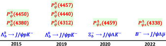
Figure 1: The summary of the observed hidden-charm pentaquark states in the recent years Aaij:2015tga ; Aaij:2019vzc ; LHCb:2020jpq ; LHCb:2022jad . Here, we provide a list of these states along with their associated production processes and the years in which they were first observed.

In 2019, LHCb conducted a more precise measurement of the $\Lambda_{b}^{0}\to J/\psi pK^{-}$ process, utilizing experimental data from both Run I and Run II Aaij:2019vzc . This analysis revealed that the previously observed $P_{\psi}^{N}(4450)$ consists of two distinct substructures, $P_{\psi}^{N}(4440)$ and $P_{\psi}^{N}(4457)$. Furthermore, a new enhancement structure named $P_{\psi}^{N}(4312)$ was discovered, which can naturally be attributed to the $\Sigma_{c}\bar{D}^{(*)}$ molecular states Li:2014gra ; Karliner:2015ina ; Wu:2010jy ; Wang:2011rga ; Yang:2011wz ; Wu:2012md ; Chen:2015loa . This updated experimental analysis from LHCb offers substantial support for the existence of the hidden-charm baryon-meson molecular pentaquark states in the realm of hadron spectroscopy Li:2014gra ; Karliner:2015ina ; Wu:2010jy ; Wang:2011rga ; Yang:2011wz ; Wu:2012md ; Chen:2015loa . However, the explorations of the hidden-charm pentaquark states, both experimentally and theoretically, remain an ongoing process.

In 2020, LHCb presented the evidence for a potential hidden-charm pentaquark structure with strangeness in the $J/\psi\Lambda$ invariant mass spectrum of the $\Xi_{b}\to J/\psi\Lambda K^{-}$ process LHCb:2020jpq , which was named $P_{\psi s}^{\Lambda}(4459)$. To date, the experimental measurement has not determined its spin-parity quantum number. Subsequently, in 2022, LHCb reported a new hidden-charm pentaquark structure with strangeness, $P_{\psi s}^{\Lambda}(4338)$, observed in the $B^{-}\to J/\psi\Lambda\bar{p}$ process by analyzing the $J/\psi\Lambda$ invariant mass spectrum LHCb:2022jad . The preferred spin-parity quantum number for this state is $J^{P}=1/2^{-}$.

For revealing the properties of these observed hidden-charm pentaquark structures with strangeness like $P_{\psi s}^{\Lambda}(4459)$ LHCb:2020jpq and $P_{\psi s}^{\Lambda}(4338)$ LHCb:2022jad , theoretical studies, employing the hadronic molecule scenario, have been proposed in Refs. Chen:2016ryt ; Wu:2010vk ; Hofmann:2005sw ; Anisovich:2015zqa ; Wang:2015wsa ; Feijoo:2015kts ; Lu:2016roh ; Xiao:2019gjd ; Shen:2020gpw ; Chen:2015sxa ; Zhang:2020cdi ; Wang:2019nvm ; Weng:2019ynv ; Paryev:2023icm ; Azizi:2023foj ; Wang:2022neq ; Wang:2022mxy ; Karliner:2022erb ; Yan:2022wuz ; Meng:2022wgl ; Ozdem:2023htj ; Feijoo:2022rxf ; Garcilazo:2022edi ; Yang:2022ezl ; Zhu:2022wpi ; Chen:2022wkh ; Ortega:2022uyu ; Giachino:2022pws ; Nakamura:2022jpd ; Wang:2022tib ; Ozdem:2022kei ; Xiao:2022csb ; Wang:2022gfb ; Clymton:2022qlr ; Chen:2022onm ; Chen:2021spf ; Gao:2021hmv ; Ferretti:2021zis ; Giron:2021fnl ; Cheng:2021gca ; Du:2021bgb ; Chen:2021cfl ; Hu:2021nvs ; Yang:2021pio ; Li:2021ryu ; Lu:2021irg ; Zou:2021sha ; Wang:2021itn ; Wu:2021caw ; Clymton:2021thh ; Xiao:2021rgp ; Ozdem:2021ugy ; Zhu:2021lhd ; Chen:2021tip ; Azizi:2021utt ; Dong:2021juy ; Liu:2020hcv ; Wang:2020eep ; Peng:2020hql ; Chen:2020uif ; Peng:2019wys ; Chen:2020opr ; Chen:2020kco ; Burns:2022uha . However, several puzzling phenomena arise when attempting to explain the observed $P_{\psi s}^{\Lambda}(4459)$ and $P_{\psi s}^{\Lambda}(4338)$ as the $\Xi_{c}\bar{D}^{(*)}$ molecular states Wang:2022mxy . For the $P_{\psi s}^{\Lambda}(4459)$ LHCb:2020jpq , the presence of the double peak structures slightly below the threshold of the $\Xi_{c}\bar{D}^{*}$ channel poses a challenge. Regarding the $P_{\psi s}^{\Lambda}(4338)$ LHCb:2022jad , its measured mass is close to and above the threshold of the $\Xi_{c}\bar{D}$ channel, making it difficult to assign it as the $\Xi_{c}\bar{D}$ molecular state. This difficulty arises from the requirement of the hadronic molecule explanation that the observed hadron state’s mass should be close to and below the sum of the thresholds of its constituent hadrons Chen:2016qju ; Liu:2019zoy .

To address these puzzling phenomena, further investigation into the properties of the $P_{\psi s}^{\Lambda}(4459)$ and $P_{\psi s}^{\Lambda}(4338)$ is needed. Extensive discussions on these topics have taken place in recent years Paryev:2023icm ; Azizi:2023foj ; Wang:2022neq ; Wang:2022mxy ; Karliner:2022erb ; Yan:2022wuz ; Meng:2022wgl ; Ozdem:2023htj ; Feijoo:2022rxf ; Garcilazo:2022edi ; Yang:2022ezl ; Zhu:2022wpi ; Chen:2022wkh ; Ortega:2022uyu ; Giachino:2022pws ; Nakamura:2022jpd ; Wang:2022tib ; Ozdem:2022kei ; Xiao:2022csb ; Wang:2022gfb ; Clymton:2022qlr ; Chen:2022onm ; Chen:2021spf ; Gao:2021hmv ; Ferretti:2021zis ; Giron:2021fnl ; Cheng:2021gca ; Du:2021bgb ; Chen:2021cfl ; Hu:2021nvs ; Yang:2021pio ; Li:2021ryu ; Lu:2021irg ; Zou:2021sha ; Wang:2021itn ; Wu:2021caw ; Clymton:2021thh ; Xiao:2021rgp ; Ozdem:2021ugy ; Zhu:2021lhd ; Chen:2021tip ; Azizi:2021utt ; Dong:2021juy ; Liu:2020hcv ; Wang:2020eep ; Peng:2020hql ; Chen:2020uif ; Peng:2019wys ; Chen:2020opr ; Chen:2020kco ; Burns:2022uha and should be checked in future experiments. Additionally, it is worth studying whether similar behaviors exist in other molecular $P_{\psi s}^{\Lambda}$ pentaquarks. This approach holds potential for unraveling the aforementioned puzzling phenomena. Moreover, the exploration of a novel class of molecular $P_{\psi s}^{\Lambda/\Sigma}$ pentaquarks could further enrich our knowledge in this field, providing valuable insights for future experimental searches and contributing to a more comprehensive understanding of these molecular pentaquarks.

The main focus of our study is on the $\Xi_{c}^{(\prime,*)}\bar{D}_{1}/\Xi_{c}^{(\prime,*)}\bar{D}_{2}^{*}$ systems that can be regarded as a new class of molecular pentaquark candidates, namely molecular $P_{\psi s}^{\Lambda/\Sigma}$ pentaquarks, with masses ranging approximately from 4.87 to 5.10 GeV. Here, the $D_{1}$ and $D_{2}^{*}$ states stand for the $D_{1}(2420)$ and $D_{2}^{*}(2460)$ charmed mesons listed in the Particle Data Group ParticleDataGroup:2022pth . In our calculations, we deduce the effective potentials of the $\Xi_{c}^{(\prime,*)}\bar{D}_{1}/\Xi_{c}^{(\prime,*)}\bar{D}_{2}^{*}$ systems using the one-boson-exchange (OBE) model. These potentials incorporate contributions from the exchange of the $\sigma$, $\pi$, $\eta$, $\rho$, and $\omega$ particles Chen:2016qju ; Liu:2019zoy . To ensure comprehensive and systematic results, we account for both the $S$-$D$ wave mixing effect and the coupled channel effect. This consideration enables a more extensive mass spectrum of the $\Xi_{c}^{(\prime,*)}\bar{D}_{1}/\Xi_{c}^{(\prime,*)}\bar{D}_{2}^{*}$-type hidden-charm molecular pentaquark candidates with strangeness. By employing the obtained OBE effective potentials, we can then solve the coupled channel Schrödinger equation to search for the bound state solutions. This process allows us to predict a novel class of molecular $P_{\psi s}^{\Lambda/\Sigma}$ pentaquark candidates comprising the charmed baryons $\Xi_{c}^{(\prime,*)}$ and the anticharmed mesons $\bar{D}_{1}/\bar{D}_{2}^{*}$.

This paper is organized as follows. After presenting the Introduction in Sec. I, we deduce the OBE effective potentials for the $\Xi_{c}^{(\prime,*)}\bar{D}_{1}/\Xi_{c}^{(\prime,*)}\bar{D}_{2}^{*}$ systems in Sec. II. With these obtained OBE effective potentials, we discuss the bound state properties for the $\Xi_{c}^{(\prime,*)}\bar{D}_{1}/\Xi_{c}^{(\prime,*)}\bar{D}_{2}^{*}$ systems, and predict a novel class of molecular $P_{\psi s}^{\Lambda/\Sigma}$ pentaquark candidates composed of the charmed baryons $\Xi_{c}^{(\prime,*)}$ and the anticharmed mesons $\bar{D}_{1}/\bar{D}_{2}^{*}$ in Sec. III. Finally, this work ends with the discussions and conclusions in Sec. IV.

II The deduction of the OBE effective potentials of the $\Xi_{c}^{(\prime,*)}\bar{D}_{1}/\Xi_{c}^{(\prime,*)}\bar{D}_{2}^{*}$ systems

The main task of the present work is to investigate a novel class of molecular $P_{\psi s}^{\Lambda/\Sigma}$ pentaquark candidates comprising the charmed baryons $\Xi_{c}^{(\prime,*)}$ and the anticharmed mesons $\bar{D}_{1}/\bar{D}_{2}^{*}$, so the $\Xi_{c}^{(\prime,*)}\bar{D}_{1}/\Xi_{c}^{(\prime,*)}\bar{D}_{2}^{*}$ interactions are the important inputs in the whole calculations. In this work, we deduce the effective potentials of the $\Xi_{c}^{(\prime,*)}\bar{D}_{1}/\Xi_{c}^{(\prime,*)}\bar{D}_{2}^{*}$ systems by adopting the OBE model Chen:2016qju ; Liu:2019zoy , which is one of the powerful tool to discuss the interactions between hadrons by exchanging the allowed light pseudoscalar, scalar, and vector mesons, such as $\pi$, $\eta$, $\sigma$, $\rho$, $\omega$, and so on. During the past few decades, the OBE model is widely adopted to study the hadron-hadron interactions. Especially, this model was applied to reproduce the masses of the observed $P_{\psi}^{N}$ Aaij:2019vzc and $P_{\psi s}^{\Lambda}$ LHCb:2020jpq ; LHCb:2022jad under the baryon-meson molecule picture Li:2014gra ; Karliner:2015ina ; Wu:2010jy ; Wang:2011rga ; Yang:2011wz ; Wu:2012md ; Chen:2015loa ; Paryev:2023icm ; Azizi:2023foj ; Wang:2022neq ; Wang:2022mxy ; Karliner:2022erb ; Yan:2022wuz ; Meng:2022wgl ; Ozdem:2023htj ; Feijoo:2022rxf ; Garcilazo:2022edi ; Yang:2022ezl ; Zhu:2022wpi ; Chen:2022wkh ; Ortega:2022uyu ; Giachino:2022pws ; Nakamura:2022jpd ; Wang:2022tib ; Ozdem:2022kei ; Xiao:2022csb ; Wang:2022gfb ; Clymton:2022qlr ; Chen:2022onm ; Chen:2021spf ; Gao:2021hmv ; Ferretti:2021zis ; Giron:2021fnl ; Cheng:2021gca ; Du:2021bgb ; Chen:2021cfl ; Hu:2021nvs ; Yang:2021pio ; Li:2021ryu ; Lu:2021irg ; Zou:2021sha ; Wang:2021itn ; Wu:2021caw ; Clymton:2021thh ; Xiao:2021rgp ; Ozdem:2021ugy ; Zhu:2021lhd ; Chen:2021tip ; Azizi:2021utt ; Dong:2021juy ; Liu:2020hcv ; Wang:2020eep ; Peng:2020hql ; Chen:2020uif ; Peng:2019wys ; Chen:2020opr ; Chen:2020kco ; Burns:2022uha , which encourages us to predict the $\Xi_{c}^{(\prime,*)}\bar{D}_{1}/\Xi_{c}^{(\prime,*)}\bar{D}_{2}^{*}$-type hidden-charm molecular pentaquark candidates with strangeness within the OBE model.

II.1 Effective Lagrangians

When taking the OBE model to estimate the interactions between hadrons quantitatively, the previous theoretical studies usually adopt the effective Lagrangian approach to calculate the scattering amplitudes Chen:2016qju ; Liu:2019zoy , and it is necessary to construct the relevant effective Lagrangians. For describing the $\Xi_{c}^{(\prime,*)}\bar{D}_{1}/\Xi_{c}^{(\prime,*)}\bar{D}_{2}^{*}$ interactions, the contributions from the exchange of the scalar meson $\sigma$, the pseudoscalar mesons $\pi$ and $\eta$, and the vector mesons $\rho$ and $\omega$ are considered Chen:2016qju ; Liu:2019zoy , and we need to calculate them out one by one and sum them in the concrete calculations.

For the sake of completeness, we briefly recall the properties of the baryons $\Xi_{c}^{(\prime,*)}$ and the mesons $\bar{D}_{1}/\bar{D}_{2}^{*}$, which can provide the crucial information to construct the effective Lagrangians. By taking the heavy quark spin symmetry Wise:1992hn , the total angular momentum of the light degrees of freedom $j_{\ell}$ including both the light quark spin $s_{q}$ and the orbital angular momentum $\ell$ is a good quantum number for the hadron containing the single heavy quark, and the hadronic states with the total angular momentum $J=j_{\ell}\pm 1/2$ can form the doublet, except for the case for $j_{\ell}=0$. Thus, the properties of the single heavy hadrons in the same doublet are degenerate approximatively, which can be written as the superfield to construct the effective Lagrangians. For these discussed singly charmed baryons, $\Xi_{c}$ with $J^{P}=1/2^{+}$ is the $S$-wave charmed baryon in the $\bar{3}_{F}$ flavor representation with $j_{\ell}=0$, while $\Xi_{c}^{\prime}$ with $J^{P}=1/2^{+}$ and $\Xi_{c}^{*}$ with $J^{P}=3/2^{+}$ are the $S$-wave charmed baryons in the $6_{F}$ flavor representation with $j_{\ell}=1$ ParticleDataGroup:2022pth . In general, the singly charmed baryon matrices $\mathcal{B}_{\bar{3}}$ and $\mathcal{B}_{6}^{(*)}$ are defined as Wise:1992hn ; Casalbuoni:1992gi ; Casalbuoni:1996pg ; Yan:1992gz ; Bando:1987br ; Harada:2003jx ; Chen:2017xat

$$\mathcal{B}_{\bar{3}}=\left(\begin{array}[]{ccc}0&\Lambda_{c}^{+}&\Xi_{c}^{+}\\ -\Lambda_{c}^{+}&0&\Xi_{c}^{0}\\ -\Xi_{c}^{+}&-\Xi_{c}^{0}&0\end{array}\right),\mathcal{B}_{6}^{(*)}=\left(\begin{array}[]{ccc}\Sigma_{c}^{{(*)}++}&\frac{\Sigma_{c}^{{(*)}+}}{\sqrt{2}}&\frac{\Xi_{c}^{(\prime,*)+}}{\sqrt{2}}\\ \frac{\Sigma_{c}^{{(*)}+}}{\sqrt{2}}&\Sigma_{c}^{{(*)}0}&\frac{\Xi_{c}^{(\prime,*)0}}{\sqrt{2}}\\ \frac{\Xi_{c}^{(\prime,*)+}}{\sqrt{2}}&\frac{\Xi_{c}^{(\prime,*)0}}{\sqrt{2}}&\Omega_{c}^{(*)0}\end{array}\right),$$ (2.7)

respectively. Under the heavy quark spin symmetry, the $S$-wave singly charmed baryons in $6_{F}$ flavor representation $\mathcal{B}_{6}$ and $\mathcal{B}^{*}_{6}$ can be expressed as the superfield $\mathcal{S}_{\mu}$, which is given by Wise:1992hn ; Casalbuoni:1992gi ; Casalbuoni:1996pg ; Yan:1992gz ; Bando:1987br ; Harada:2003jx ; Chen:2017xat

$$\mathcal{S}_{\mu}=-\sqrt{\frac{1}{3}}(\gamma_{\mu}+v_{\mu})\gamma^{5}\mathcal{B}_{6}+\mathcal{B}_{6\mu}^{*}.$$ (2.8)

Here, the four velocity has the form $v_{\mu}=(1,0,0,0)$ within the nonrelativistic approximation, and its conjugate field is $\bar{\mathcal{S}}_{\mu}=\mathcal{S}_{\mu}^{\dagger}\gamma^{0}$. For these focused mesons, $\bar{D}_{1}$ with $J^{P}=1^{+}$ and $\bar{D}_{2}^{*}$ with $J^{P}=2^{+}$ are the $P$-wave anticharmed mesons in the $T$ doublet with $j_{\ell}=3/2$ ParticleDataGroup:2022pth , which can be constructed as the superfield $T^{(\bar{Q})\mu}_{a}$ as follows Ding:2008gr

$$T^{(\bar{Q})\mu}_{a}=\left[\bar{D}^{*\mu\nu}_{2a}\gamma_{\nu}-\sqrt{\frac{3}{2}}\bar{D}_{1a\nu}\gamma_{5}\left(g^{\mu\nu}-\frac{1}{3}(\gamma^{\mu}-v^{\mu})\gamma^{\nu}\right)\right]\frac{1-/\!\!\!v}{2},$$

where the corresponding conjugate field is $\overline{T}^{(\bar{Q})\mu}_{a}=\gamma^{0}T_{a}^{(\bar{Q})\mu{\dagger}}\gamma^{0}$. For convenience, we take the column matrices to describe the anticharmed meson fields in the $T$ doublet, i.e., $\bar{D}_{1}=(\bar{D}_{1}^{0},\,\bar{D}_{1}^{-},\,D_{s1}^{-})^{T}$ and $\bar{D}_{2}^{*}=(\bar{D}_{2}^{*0},\,\bar{D}_{2}^{*-},\,D_{s2}^{*-})^{T}$.

Now we move on to construct the effective Lagrangians adopted in the present work by taking into account the symmetry requirements. With the help of the constraints of the heavy quark symmetry, the chiral symmetry, and the hidden local symmetry Casalbuoni:1992gi ; Casalbuoni:1996pg ; Yan:1992gz ; Harada:2003jx ; Bando:1987br , the effective Lagrangians related to the interactions between the singly charmed baryons $\Xi_{c}^{(\prime,*)}$ and the light scalar, pseudoscalar, and vector mesons are constructed as Wise:1992hn ; Casalbuoni:1992gi ; Casalbuoni:1996pg ; Yan:1992gz ; Bando:1987br ; Harada:2003jx ; Chen:2017xat

$$\mathcal{L}_{\mathcal{B}_{\bar{3}}\mathcal{B}_{\bar{3}}\mathcal{E}} = l_{B}\langle\bar{\mathcal{B}}_{\bar{3}}\sigma\mathcal{B}_{\bar{3}}\rangle+i\beta_{B}\langle\bar{\mathcal{B}}_{\bar{3}}v^{\mu}(\mathcal{V}_{\mu}-\rho_{\mu})\mathcal{B}_{\bar{3}}\rangle,$$ (2.10)

$$\mathcal{L}_{\mathcal{S}\mathcal{S}\mathcal{E}} = l_{S}\langle\bar{\mathcal{S}}_{\mu}\sigma\mathcal{S}^{\mu}\rangle-\frac{3}{2}g_{1}\varepsilon^{\mu\nu\lambda\kappa}v_{\kappa}\langle\bar{\mathcal{S}}_{\mu}\mathcal{A}_{\nu}\mathcal{S}_{\lambda}\rangle$$

$$+i\beta_{S}\langle\bar{\mathcal{S}}_{\mu}v_{\alpha}\left(\mathcal{V}^{\alpha}-\rho^{\alpha}\right)\mathcal{S}^{\mu}\rangle+\lambda_{S}\langle\bar{\mathcal{S}}_{\mu}F^{\mu\nu}(\rho)\mathcal{S}_{\nu}\rangle,$$

$$\mathcal{L}_{\mathcal{B}_{\bar{3}}\mathcal{S}\mathcal{E}} = ig_{4}\langle\bar{\mathcal{S}^{\mu}}\mathcal{A}_{\mu}\mathcal{B}_{\bar{3}}\rangle+i\lambda_{I}\varepsilon^{\mu\nu\lambda\kappa}v_{\mu}\langle\bar{\mathcal{S}}_{\nu}F_{\lambda\kappa}\mathcal{B}_{\bar{3}}\rangle+h.c.,$$

where the notation $\mathcal{E}$ in the subscript stands for the exchanged light mesons. Furthermore, the effective Lagrangians depicting the interactions of the anticharmed mesons in the $T$ doublet $\bar{D}_{1}/\bar{D}_{2}^{*}$ and the light scalar, pseudoscalar, and vector mesons can be constructed as Ding:2008gr

$$\mathcal{L}_{\bar{T}\bar{T}\mathcal{E}} = g^{\prime\prime}_{\sigma}\langle\overline{T}^{(\bar{Q})\mu}_{a}\sigma T^{\,({\bar{Q}})}_{a\mu}\rangle+ik\langle\overline{T}^{(\bar{Q})\mu}_{b}{\cal A}\!\!\!/_{ba}\gamma_{5}{T}^{\,(\bar{Q})}_{a\mu}\rangle$$ (2.13)

$$-i\beta^{\prime\prime}\langle\overline{T}^{(\bar{Q})}_{b\lambda}v^{\mu}({\cal V}_{\mu}-\rho_{\mu})_{ba}T^{\,(\bar{Q})\lambda}_{a}\rangle$$

$$+i\lambda^{\prime\prime}\langle\overline{T}^{(\bar{Q})}_{b\lambda}\sigma^{\mu\nu}F_{\mu\nu}(\rho)_{ba}T^{\,(\bar{Q})\lambda}_{a}\rangle.$$

In the constructed effective Lagrangians, the axial current $\mathcal{A}_{\mu}$ and the vector current ${\mathcal{V}}_{\mu}$ are given by

$${\mathcal{A}}_{\mu}=\frac{1}{2}\left(\xi^{\dagger}\partial_{\mu}\xi-\xi\partial_{\mu}\xi^{\dagger}\right),~{}~{}~{}~{}{\mathcal{V}}_{\mu}=\frac{1}{2}\left(\xi^{\dagger}\partial_{\mu}\xi+\xi\partial_{\mu}\xi^{\dagger}\right),$$ (2.14)

respectively. Here, the pseudo-Goldstone meson field is $\xi=e^{i\mathbb{P}/f_{\pi}}$, and $f_{\pi}$ stands for the pion decay constant with $f_{\pi}=0.132~{}{\rm GeV}$. Furthermore, $\mathcal{A}_{\mu}$ and ${\mathcal{V}}_{\mu}$ at the leading order of $\xi$ can be simplified to be

$$\mathcal{A}_{\mu}=\frac{i}{f_{\pi}}\partial_{\mu}{\mathbb{P}},~{}~{}~{}~{}~{}\mathcal{V}_{\mu}=0.$$ (2.15)

In addition, we define the vector meson field $\rho_{\mu}$ and the vector meson field strength tensor $F_{\mu\nu}$ as

$$\rho_{\mu}=\frac{i{g_{V}}}{\sqrt{2}}\mathbb{V}_{\mu},~{}~{}~{}~{}~{}F_{\mu\nu} = \partial_{\mu}\rho_{\nu}-\partial_{\nu}\rho_{\mu}+\left[\rho_{\mu},\rho_{\nu}\right],$$ (2.16)

respectively. Explicitly, the light pseudoscalar meson matrix $\mathbb{P}$ and the light vector meson matrix $\mathbb{V}_{\mu}$ are defined as

$${\mathbb{P}} = {\left(\begin{array}[]{ccc}\frac{\pi^{0}}{\sqrt{2}}+\frac{\eta}{\sqrt{6}}&\pi^{+}&K^{+}\\ \pi^{-}&-\frac{\pi^{0}}{\sqrt{2}}+\frac{\eta}{\sqrt{6}}&K^{0}\\ K^{-}&\bar{K}^{0}&-\sqrt{\frac{2}{3}}\eta\end{array}\right)},$$ (2.20)

$${\mathbb{V}}_{\mu} = {\left(\begin{array}[]{ccc}\frac{\rho^{0}}{\sqrt{2}}+\frac{\omega}{\sqrt{2}}&\rho^{+}&K^{*+}\\ \rho^{-}&-\frac{\rho^{0}}{\sqrt{2}}+\frac{\omega}{\sqrt{2}}&K^{*0}\\ K^{*-}&\bar{K}^{*0}&\phi\end{array}\right)}_{\mu},$$ (2.24)

respectively.

Combined with the constructed effective Lagrangians and the defined physical quantities, the concrete effective Lagrangians can be further obtained after expanding the above constructed effective Lagrangians to the leading order of $\xi$, which are needed in the realistic calculations. Specifically, the effective Lagrangians for the heavy hadrons $\Xi_{c}^{(\prime,*)}/\bar{D}_{1}/\bar{D}_{2}^{*}$ coupling with the light scalar meson $\sigma$ are expressed as

$$\mathcal{L}_{\mathcal{B}_{\bar{3}}\mathcal{B}_{\bar{3}}\sigma} = l_{B}\langle\bar{\mathcal{B}}_{\bar{3}}\sigma\mathcal{B}_{\bar{3}}\rangle,$$ (2.25)

$$\mathcal{L}_{\mathcal{B}_{6}^{(*)}\mathcal{B}_{6}^{(*)}\sigma} = -l_{S}\langle\bar{\mathcal{B}}_{6}\sigma\mathcal{B}_{6}\rangle+l_{S}\langle\bar{\mathcal{B}}_{6\mu}^{*}\sigma\mathcal{B}_{6}^{*\mu}\rangle$$ (2.26)

$$-\frac{l_{S}}{\sqrt{3}}\langle\bar{\mathcal{B}}_{6\mu}^{*}\sigma\left(\gamma^{\mu}+v^{\mu}\right)\gamma^{5}\mathcal{B}_{6}\rangle+h.c.,$$

$$\mathcal{L}_{\bar{T}\bar{T}\sigma} = -2g_{\sigma}^{\prime\prime}\bar{D}_{1a\mu}\bar{D}^{\mu\dagger}_{1a}\sigma+2g_{\sigma}^{\prime\prime}\bar{D}^{*\dagger}_{2a\mu\nu}\bar{D}^{*\mu\nu}_{2a}\sigma,$$ (2.27)

and the effective Lagrangians depicting the interactions of the heavy hadrons $\Xi_{c}^{(\prime,*)}/\bar{D}_{1}/\bar{D}_{2}^{*}$ and the light pseudoscalar mesons $\mathbb{P}$ are

$$\mathcal{L}_{\mathcal{B}_{6}^{(*)}\mathcal{B}_{6}^{(*)}\mathbb{P}} = i\frac{g_{1}}{2f_{\pi}}\varepsilon^{\mu\nu\lambda\kappa}v_{\kappa}\langle\bar{\mathcal{B}}_{6}\gamma_{\mu}\gamma_{\lambda}\partial_{\nu}\mathbb{P}\mathcal{B}_{6}\rangle$$

$$-i\frac{3g_{1}}{2f_{\pi}}\varepsilon^{\mu\nu\lambda\kappa}v_{\kappa}\langle\bar{\mathcal{B}}_{6\mu}^{*}\partial_{\nu}\mathbb{P}\mathcal{B}_{6\lambda}^{*}\rangle$$

$$+i\frac{\sqrt{3}g_{1}}{2f_{\pi}}v_{\kappa}\varepsilon^{\mu\nu\lambda\kappa}\langle\bar{\mathcal{B}}_{6\mu}^{*}\partial_{\nu}\mathbb{P}{\gamma_{\lambda}\gamma^{5}}\mathcal{B}_{6}\rangle+h.c.,$$

$$\mathcal{L}_{\mathcal{B}_{\bar{3}}\mathcal{B}_{6}^{(*)}\mathbb{P}} = -\sqrt{\frac{1}{3}}\frac{g_{4}}{f_{\pi}}\langle\bar{\mathcal{B}}_{6}\gamma^{5}\left(\gamma^{\mu}+v^{\mu}\right)\partial_{\mu}\mathbb{P}\mathcal{B}_{\bar{3}}\rangle$$ (2.29)

$$-\frac{g_{4}}{f_{\pi}}\langle\bar{\mathcal{B}}_{6\mu}^{*}\partial^{\mu}\mathbb{P}\mathcal{B}_{\bar{3}}\rangle+h.c.,$$

$$\mathcal{L}_{\bar{T}\bar{T}\mathbb{P}} = -\frac{5ik}{3f_{\pi}}\varepsilon^{\mu\nu\rho\tau}v_{\nu}\bar{D}^{{\dagger}}_{1a\rho}\bar{D}_{1b\tau}\partial_{\mu}\mathbb{P}_{ba}$$

$$+\frac{2ik}{f_{\pi}}\varepsilon^{\mu\nu\rho\tau}v_{\nu}\bar{D}^{*\alpha{\dagger}}_{2a\rho}\bar{D}^{*}_{2b\alpha\tau}\partial_{\mu}\mathbb{P}_{ba}$$

$$+\sqrt{\frac{2}{3}}\frac{k}{f_{\pi}}\left(\bar{D}^{\dagger}_{1a\mu}\bar{D}^{*\mu\lambda}_{2b}+\bar{D}_{1b\mu}\bar{D}^{*\mu\lambda\dagger}_{2a}\right)\partial_{\lambda}\mathbb{P}_{ba},$$

and the effective Lagrangians describing the interactions between the heavy hadrons $\Xi_{c}^{(\prime,*)}/\bar{D}_{1}/\bar{D}_{2}^{*}$ and the light vector mesons $\mathbb{V}$ are

$$\mathcal{L}_{\mathcal{B}_{\bar{3}}\mathcal{B}_{\bar{3}}\mathbb{V}} = \frac{1}{\sqrt{2}}\beta_{B}g_{V}\langle\bar{\mathcal{B}}_{\bar{3}}v\cdot\mathbb{V}\mathcal{B}_{\bar{3}}\rangle,$$ (2.31)

$$\mathcal{L}_{\mathcal{B}_{6}^{(*)}\mathcal{B}_{6}^{(*)}\mathbb{V}} = -\frac{\beta_{S}g_{V}}{\sqrt{2}}\langle\bar{\mathcal{B}}_{6}v\cdot\mathbb{V}\mathcal{B}_{6}\rangle+\frac{\beta_{S}g_{V}}{\sqrt{2}}\langle\bar{\mathcal{B}}_{6\mu}^{*}v\cdot{V}\mathcal{B}_{6}^{*\mu}\rangle$$

$$-i\frac{\lambda_{S}g_{V}}{3\sqrt{2}}\langle\bar{\mathcal{B}}_{6}\gamma_{\mu}\gamma_{\nu}\left(\partial^{\mu}\mathbb{V}^{\nu}-\partial^{\nu}\mathbb{V}^{\mu}\right)\mathcal{B}_{6}\rangle$$

$$+i\frac{\lambda_{S}g_{V}}{\sqrt{2}}\langle\bar{\mathcal{B}}_{6\mu}^{*}\left(\partial^{\mu}\mathbb{V}^{\nu}-\partial^{\nu}\mathbb{V}^{\mu}\right)\mathcal{B}_{6\nu}^{*}\rangle$$

$$-i\frac{\lambda_{S}g_{V}}{\sqrt{6}}\langle\bar{\mathcal{B}}_{6\mu}^{*}\left(\partial^{\mu}\mathbb{V}^{\nu}-\partial^{\nu}\mathbb{V}^{\mu}\right)\left(\gamma_{\nu}+v_{\nu}\right)\gamma^{5}\mathcal{B}_{6}\rangle$$

$$-\frac{\beta_{S}g_{V}}{\sqrt{6}}\langle\bar{\mathcal{B}}_{6\mu}^{*}v\cdot\mathbb{V}\left(\gamma^{\mu}+v^{\mu}\right)\gamma^{5}\mathcal{B}_{6}\rangle+h.c.,$$

$$\mathcal{L}_{\mathcal{B}_{\bar{3}}\mathcal{B}_{6}^{(*)}\mathbb{V}} = -\frac{\lambda_{I}g_{V}}{\sqrt{2}}\varepsilon^{\mu\nu\lambda\kappa}v_{\mu}\langle\bar{\mathcal{B}}_{6\nu}^{*}\left(\partial_{\lambda}\mathbb{V}_{\kappa}-\partial_{\kappa}\mathbb{V}_{\lambda}\right)\mathcal{B}_{\bar{3}}\rangle$$

$$-\frac{\lambda_{I}g_{V}}{\sqrt{6}}\varepsilon^{\mu\nu\lambda\kappa}v_{\mu}\langle\bar{\mathcal{B}}_{6}\gamma^{5}\gamma_{\nu}\left(\partial_{\lambda}\mathbb{V}_{\kappa}-\partial_{\kappa}\mathbb{V}_{\lambda}\right)\mathcal{B}_{\bar{3}}\rangle+h.c.,$$

$$\mathcal{L}_{\bar{T}\bar{T}\mathbb{V}} = \sqrt{2}\beta^{\prime\prime}g_{V}\left(v\cdot\mathbb{V}_{ba}\right)\bar{D}_{1b\mu}\bar{D}^{\mu\dagger}_{1a}$$ (2.34)

$$+\frac{5\sqrt{2}i\lambda^{\prime\prime}g_{V}}{3}\left(\bar{D}^{\nu}_{1b}\bar{D}^{\mu\dagger}_{1a}-\bar{D}^{\nu\dagger}_{1a}\bar{D}^{\mu}_{1b}\right)\partial_{\mu}\mathbb{V}_{ba\nu}$$

$$-\sqrt{2}\beta^{\prime\prime}g_{V}\left(v\cdot\mathbb{V}_{ba}\right)\bar{D}_{2b}^{*\lambda\nu}\bar{D}^{*\dagger}_{2a{\lambda\nu}}$$

$$+2\sqrt{2}i\lambda^{\prime\prime}g_{V}\left(\bar{D}^{*\lambda\nu\dagger}_{2a}\bar{D}^{*\mu}_{2b\lambda}-\bar{D}^{*\lambda\nu}_{2b}\bar{D}^{*\mu\dagger}_{2a\lambda}\right)\partial_{\mu}\mathbb{V}_{ba\nu}$$

$$+\frac{i\beta^{\prime\prime}g_{V}}{\sqrt{3}}\varepsilon^{\lambda\alpha\rho\tau}v_{\rho}\left(v\cdot\mathbb{V}_{ba}\right)\left(\bar{D}^{\dagger}_{1a\alpha}\bar{D}^{*}_{2b\lambda\tau}-\bar{D}_{1b\alpha}\bar{D}^{\dagger*}_{2a\lambda\tau}\right)$$

$$+\frac{2\lambda^{\prime\prime}g_{V}}{\sqrt{3}}\left[3\varepsilon^{\mu\lambda\nu\tau}v_{\lambda}\left(\bar{D}^{\alpha\dagger}_{1a}\bar{D}^{*}_{2b\alpha\tau}+\bar{D}^{\alpha}_{1b}\bar{D}^{*\dagger}_{2a\alpha\tau}\right)\partial_{\mu}\mathbb{V}_{ba\nu}\right.$$

$$\left.+2\varepsilon^{\lambda\alpha\rho\nu}v_{\rho}\left(\bar{D}^{\dagger}_{1a\alpha}\bar{D}^{*\mu}_{2b\lambda}+\bar{D}_{1b\alpha}\bar{D}^{\dagger\mu*}_{2a\lambda}\right)\right.$$

$$\left.\times\left(\partial_{\mu}\mathbb{V}_{ba\nu}-\partial_{\nu}\mathbb{V}_{ba\mu}\right)\right].$$

For these obtained effective Lagrangians, the coupling constants are the important input parameters to describe the strengths of the interaction vertices quantitatively. In general, we can extract the coupling constants through reproducing the experimental data when there exists the relevant experimental information, and the coupling constants also can be deduced by taking the theoretical models and approaches. Furthermore, the phase factors of the related coupling constants can be fixed with the help of the quark model Riska:2000gd . In the following numerical analysis, we take $l_{B}=-3.65$, $l_{S}=6.20$, $g_{\sigma}^{\prime\prime}=-0.76$, $g_{1}=0.94$, $g_{4}=1.06$, $k=-0.59$, $\beta_{B}g_{V}=-6.00$, $\beta_{S}g_{V}=12.00$, $\lambda_{I}g_{V}=-6.80~{}\rm{GeV^{-1}}$, $\lambda_{S}g_{V}=19.20~{}\rm{GeV^{-1}}$, $\beta^{\prime\prime}g_{V}=5.25$, and $\lambda^{\prime\prime}g_{V}=3.27~{}\rm{GeV^{-1}}$, which were given in Refs. Wang:2022mxy ; Chen:2017xat ; Chen:2019asm ; Chen:2020kco ; Wang:2020bjt ; Wang:2019nwt ; Chen:2018pzd ; Wang:2021hql ; Wang:2019aoc ; Wang:2021ajy ; Wang:2021yld ; Wang:2021aql ; Yang:2021sue ; Wang:2020dya . In the past decades, these coupling constants are widely applied to discuss the hadron-hadron interactions, especially after the observed $P_{\psi}^{N}$ and $P_{\psi s}^{\Lambda}$ Aaij:2015tga ; Aaij:2019vzc ; LHCb:2020jpq ; LHCb:2022jad .

II.2 The OBE potentials

Now we illustrate how to deduce the OBE effective potentials for the $\Xi_{c}^{(\prime,*)}\bar{D}_{1}/\Xi_{c}^{(\prime,*)}\bar{D}_{2}^{*}$ systems based on the constructed effective Lagrangians Wang:2022mxy ; Wang:2020dya ; Wang:2019nwt ; Wang:2019aoc ; Wang:2020bjt ; Wang:2021hql ; Chen:2018pzd ; Yang:2021sue ; Wang:2021ajy ; Wang:2021yld ; Wang:2021aql . In the context of the effective Lagrangian approach, we can calculate the scattering amplitude $\mathcal{M}^{h_{1}h_{2}\to h_{3}h_{4}}(\bm{q})$ of the $h_{1}h_{2}\to h_{3}h_{4}$ scattering process by exchanging the allowed light mesons $\mathcal{E}$ with the help of the Feynman rule, which can be obtained by the following relation Wang:2021ajy

$$i\mathcal{M}^{h_{1}h_{2}\to h_{3}h_{4}}(\bm{q})=\sum_{\mathcal{E}=\sigma,\,\mathbb{P},\,\mathbb{V}}i\Gamma^{h_{1}h_{3}\mathcal{E}}_{(\mu)}P_{\mathcal{E}}^{(\mu\nu)}i\Gamma^{h_{2}h_{4}\mathcal{E}}_{(\nu)}.$$ (2.35)

Here, $P_{\mathcal{E}}^{(\mu\nu)}$ is the propagator of the exchanged light meson, which can be defined as

$$P_{\sigma} = \frac{i}{q^{2}-m_{\sigma}^{2}},~{}~{}~{}~{}~{}~{}~{}~{}~{}~{}~{}~{}~{}~{}~{}~{}~{}~{}~{}~{}P_{{\mathbb{P}}}=\frac{i}{q^{2}-m_{{\mathbb{P}}}^{2}},$$

$$P_{\mathbb{V}}^{\mu\nu} = -i\frac{g^{\mu\nu}-{q^{\mu}q^{\nu}}/{m_{\mathbb{V}}^{2}}}{q^{2}-m_{\mathbb{V}}^{2}}$$ (2.36)

for the scalar, pseudoscalar, and vector mesons, respectively. Here, $q$ and $m_{\mathcal{E}}$ are the four momentum and the mass of the exchanged light meson, respectively. $\Gamma^{h_{1}h_{3}\mathcal{E}}_{(\mu)}$ and $\Gamma^{h_{2}h_{4}\mathcal{E}}_{(\nu)}$ are the corresponding interaction vertices for the $h_{1}h_{2}\to h_{3}h_{4}$ scattering process, which can be extracted from the constructed effective Lagrangians $\mathcal{L}_{h_{1}h_{3}\mathcal{E}}$ and $\mathcal{L}_{h_{2}h_{4}\mathcal{E}}$, respectively. In the above subsection, we have constructed the effective Lagrangians adopted in the present work. In Appendix A, we present the related interaction vertices. In addition, we also need to define the normalization relations for the heavy hadrons $\Xi_{c}^{(\prime,*)}/\bar{D}_{1}/\bar{D}_{2}^{*}$ to write down the scattering amplitude $\mathcal{M}^{h_{1}h_{2}\to h_{3}h_{4}}(\bm{q})$. In our calculations, we take the normalization relations for the heavy hadrons $\Xi_{c}^{(\prime,*)}/\bar{D}_{1}/\bar{D}_{2}^{*}$ as Ding:2008gr

$$\langle 0|\Xi_{c}^{(\prime)}|cqs\left({1}/{2}^{+}\right)\rangle = \sqrt{2m_{\Xi_{c}^{(\prime)}}}{\left(\chi_{\frac{1}{2}m},\frac{\bm{\sigma}\cdot\bm{p}}{2m_{\Xi_{c}^{(\prime)}}}\chi_{\frac{1}{2}m}\right)^{T}},$$

$$\langle 0|\Xi_{c}^{*\mu}|cqs\left({3}/{2}^{+}\right)\rangle = \sqrt{2m_{\Xi_{c}^{*}}}\left(\Phi_{\frac{3}{2}m}^{\mu},\frac{\bm{\sigma}\cdot\bm{p}}{2m_{\Xi_{c}^{*}}}\Phi_{\frac{3}{2}m}^{\mu}\right)^{T},$$

$$\langle 0|\bar{D}_{1}^{\mu}|\bar{c}q(1^{+})\rangle = \sqrt{m_{\bar{D}_{1}}}\epsilon^{\mu},$$

$$\langle 0|\bar{D}_{2}^{*\mu\nu}|\bar{c}q(2^{+})\rangle = \sqrt{m_{\bar{D}_{2}^{*}}}\zeta^{\mu\nu},$$ (2.37)

respectively. Here, $m_{i}$ ($i=\Xi_{c},\,\Xi_{c}^{\prime},\,\Xi_{c}^{*},\,\bar{D}_{1},\,\bar{D}_{2}^{*}$) is the mass of the heavy hadron $i$, while $\bm{\sigma}$ and $\bm{p}$ are the Pauli matrix and the momentum of the charmed baryon, respectively. $\epsilon^{\mu}$ and $\zeta^{\mu\nu}$ are the polarization vector and the polarization tensor, respectively. In the static limit, the polarization vector $\epsilon_{m}^{\mu}\,(m=0,\,\pm 1)$ can be explicitly written as $\epsilon_{-1}^{\mu}=\left(0,\,-1,\,i,\,0\right)/\sqrt{2}$, $\epsilon_{0}^{\mu}=\left(0,0,0,-1\right)$, and $\epsilon_{+1}^{\mu}=\left(0,\,1,\,i,\,0\right)/\sqrt{2}$, while the polarization tensor $\zeta^{\mu\nu}_{m}$ can be constructed by the coupling of both polarization vectors $\epsilon^{\mu}_{m_{1}}$ and $\epsilon^{\nu}_{m_{2}}$ Cheng:2010yd , which can be represented as

$$\zeta^{\mu\nu}_{m}=\sum_{m_{1},m_{2}}C^{2,m}_{1m_{1},1m_{2}}\epsilon^{\mu}_{m_{1}}\epsilon^{\nu}_{m_{2}},$$ (2.38)

where the Clebsch-Gordan coefficient $C^{2,m}_{1m_{1},1m_{2}}$ is used to describe the related coupling. In addition, the spin wave function of the charmed baryon $\Xi_{c}^{(\prime)}$ is defined as $\chi_{\frac{1}{2}m}$, and the polarization tensor $\Phi_{\frac{3}{2}m}^{\mu}$ of the charmed baryon $\Xi_{c}^{*}$ can be constructed by the coupling of the spin wave function $\chi_{\frac{1}{2}m_{1}}$ and the polarization vector $\epsilon_{m_{2}}^{\mu}$, which can be given by

$$\Phi_{\frac{3}{2}m}^{\mu}=\sum_{m_{1},m_{2}}C^{\frac{3}{2},m}_{\frac{1}{2}m_{1},1m_{2}}\chi_{\frac{1}{2}m_{1}}\epsilon_{m_{2}}^{\mu}.$$ (2.39)

Up to now, we have obtained the scattering amplitude $\mathcal{M}^{h_{1}h_{2}\to h_{3}h_{4}}(\bm{q})$ of the $h_{1}h_{2}\to h_{3}h_{4}$ process. Taking into account both the Breit approximation and the nonrelativistic normalization Breitapproximation , the effective potential in the momentum space $\mathcal{V}_{E}^{h_{1}h_{2}\to h_{3}h_{4}}(\bm{q})$ can be extracted based on the obtained scattering amplitude $\mathcal{M}^{h_{1}h_{2}\to h_{3}h_{4}}(\bm{q})$. To be more specific, the relation between the effective potential in the momentum space $\mathcal{V}^{h_{1}h_{2}\to h_{3}h_{4}}(\bm{q})$ and the scattering amplitude $\mathcal{M}^{h_{1}h_{2}\to h_{3}h_{4}}(\bm{q})$ can be written in a general form of Breitapproximation

$$\mathcal{V}_{E}^{h_{1}h_{2}\to h_{3}h_{4}}(\bm{q}) = -\frac{\mathcal{M}^{h_{1}h_{2}\to h_{3}h_{4}}(\bm{q})}{4\sqrt{m_{h_{1}}m_{h_{2}}m_{h_{3}}m_{h_{4}}}},$$ (2.40)

where $m_{h_{i}}\,(i=1,\,2,\,3,\,4)$ is the mass of the hadron $h_{i}$. The obtained effective potential in the momentum space $\mathcal{V}_{E}^{h_{1}h_{2}\to h_{3}h_{4}}(\bm{q})$ is the function of the momentum of the exchanged light mesons $\bm{q}$, but we discuss the bound state properties of the $\Xi_{c}^{(\prime,*)}\bar{D}_{1}/\Xi_{c}^{(\prime,*)}\bar{D}_{2}^{*}$ systems by solving the Schr$\ddot{\rm o}$dinger equation in the coordinate space in the present work. Thus, we need to obtain the effective potentials in the coordinate space $\mathcal{V}_{E}^{h_{1}h_{2}\to h_{3}h_{4}}(\bm{r})$ for these discussed systems. After taking the Fourier transformation for the effective potential in the momentum space $\mathcal{V}_{E}^{h_{1}h_{2}\to h_{3}h_{4}}(\bm{q})$ together with the form factor, we can deduce the effective potential in the coordinate space $\mathcal{V}_{E}^{h_{1}h_{2}\to h_{3}h_{4}}(\bm{r})$ by the following relation

$$\mathcal{V}_{E}^{h_{1}h_{2}\to h_{3}h_{4}}(\bm{r})=\int\frac{d^{3}\bm{q}}{(2\pi)^{3}}e^{i\bm{q}\cdot\bm{r}}\mathcal{V}_{E}^{h_{1}h_{2}\to h_{3}h_{4}}(\bm{q})\mathcal{F}^{2}(q^{2},m_{\mathcal{E}}^{2}).$$

Given that the conventional baryons and mesons are not point particles, the form factor $\mathcal{F}(q^{2},m_{\mathcal{E}}^{2})$ was introduced in each interaction vertex for the Feynman diagram, which can be taken to compensate the roles of the inner structure of the discussed hadrons and the off shell of the exchanged light mesons. Generally speaking, there exist many different kinds of form factors Chen:2016qju , and we choose the monopole-type form factor in the present work, i.e.,

$$\mathcal{F}(q^{2},m_{\mathcal{E}}^{2})=\frac{\Lambda^{2}-m_{\mathcal{E}}^{2}}{\Lambda^{2}-q^{2}},$$ (2.42)

which is similar to the case for studying the bound state properties of the deuteron Tornqvist:1993ng ; Tornqvist:1993vu . In the above monopole-type form factor, $\Lambda$ is the cutoff parameter, and we define the mass and the four momentum of the exchanged light meson as $m_{\mathcal{E}}$ and $q$, respectively.

In the following, we further discuss the related wave functions for the $\Xi_{c}^{(\prime,*)}\bar{D}_{1}/\Xi_{c}^{(\prime,*)}\bar{D}_{2}^{*}$ systems, which contain the color, the spin-orbital, the flavor, and the spatial wave functions. For the hadronic molecular states composed of two color-singlet hadrons, the color wave function is simply taken as unity. The spin-orbital and flavor wave functions can be constructed by taking into account the coupling of the constituent hadrons, which can be used to calculate the operator matrix elements and the isospin factors for the OBE effective potentials, respectively. In addition, the spatial wave function can be obtained by solving the Schr$\ddot{\rm o}$dinger equation, which can be regarded as the important inputs to study their properties in future, such as the strong decay properties, the electromagnetic properties, and so on. The spin-orbital wave functions $|{}^{2S+1}L_{J}\rangle$ of the $\Xi_{c}^{(\prime,*)}\bar{D}_{1}/\Xi_{c}^{(\prime,*)}\bar{D}_{2}^{*}$ systems can be constructed as

$$\Xi_{c}^{(\prime)}\bar{D}_{1}:|{}^{2S+1}L_{J}\rangle = \sum_{m,m^{\prime},m_{S}m_{L}}C^{S,m_{S}}_{\frac{1}{2}m,1m^{\prime}}C^{J,M}_{Sm_{S},Lm_{L}}\chi_{\frac{1}{2}m}\epsilon^{m^{\prime}}|Y_{L,m_{L}}\rangle,$$

$$\Xi_{c}^{(\prime)}\bar{D}_{2}^{*}:|{}^{2S+1}L_{J}\rangle = \sum_{m,m^{\prime\prime},m_{S}m_{L}}C^{S,m_{S}}_{\frac{1}{2}m,2m^{\prime}}C^{J,M}_{Sm_{S},Lm_{L}}\chi_{\frac{1}{2}m}\zeta^{m^{\prime}}|Y_{L,m_{L}}\rangle,$$

$$\Xi_{c}^{*}\bar{D}_{1}:|{}^{2S+1}L_{J}\rangle = \sum_{m,m^{\prime},m_{S}m_{L}}C^{S,m_{S}}_{\frac{3}{2}m,1m^{\prime}}C^{J,M}_{Sm_{S},Lm_{L}}\Phi_{\frac{3}{2}m}\epsilon^{m^{\prime}}|Y_{L,m_{L}}\rangle,$$

$$\Xi_{c}^{*}\bar{D}_{2}^{*}:|{}^{2S+1}L_{J}\rangle = \sum_{m,m^{\prime},m_{S}m_{L}}C^{S,m_{S}}_{\frac{3}{2}m,2m^{\prime}}C^{J,M}_{Sm_{S},Lm_{L}}\Phi_{\frac{3}{2}m}\zeta^{m^{\prime}}|Y_{L,m_{L}}\rangle,$$

where $|Y_{L,m_{L}}\rangle$ is the spherical harmonics function. Since the isospin quantum numbers for the charmed baryons $\Xi_{c}^{(\prime,*)}$ and the charmed mesons $D_{1}/D_{2}^{*}$ are $1/2$, the $\Xi_{c}^{(\prime,*)}\bar{D}_{1}/\Xi_{c}^{(\prime,*)}\bar{D}_{2}^{*}$ systems have the isospin quantum numbers either 0 or 1, where we summarize the flavor wave functions of the isoscalar and isovector $\Xi_{c}^{(\prime,*)}\bar{D}_{1}/\Xi_{c}^{(\prime,*)}\bar{D}_{2}^{*}$ systems in Table 1. Finally, we can derive the OBE effective potentials in the coordinate space for the $\Xi_{c}^{(\prime,*)}\bar{D}_{1}/\Xi_{c}^{(\prime,*)}\bar{D}_{2}^{*}$ systems by the standard strategy listed above, which is collected in Appendix B.

Table 1: The flavor wave functions of the isoscalar and isovector $\Xi_{c}^{(\prime,*)}\bar{D}_{1}/\Xi_{c}^{(\prime,*)}\bar{D}_{2}^{*}$ systems. Here, the notation $\mathcal{D}$ stands for either $D_{1}$ or $D_{2}^{*}$ meson, while $I$ and $I_{3}$ are used to denote the isospin and its third component of the discussed system, respectively.

Isospins	$\left|I,I_{3}\right\rangle$	Flavor wave functions
Isoscalar	$\left|0,0\right\rangle$	$\frac{1}{\sqrt{2}}\left|\Xi_{c}^{(\prime,*)+}\mathcal{D}^{-}\right\rangle-\frac{1}{\sqrt{2}}\left|\Xi_{c}^{(\prime,*)0}\bar{\mathcal{D}}^{0}\right\rangle$
Isovector	$\left|1,1\right\rangle$	$\left|\Xi_{c}^{(\prime,*)+}\bar{\mathcal{D}}^{0}\right\rangle$
	$\left|1,0\right\rangle$	$\frac{1}{\sqrt{2}}\left|\Xi_{c}^{(\prime,*)+}\mathcal{D}^{-}\right\rangle+\frac{1}{\sqrt{2}}\left|\Xi_{c}^{(\prime,*)0}\bar{\mathcal{D}}^{0}\right\rangle$
	$\left|1,-1\right\rangle$	$\left|\Xi_{c}^{(\prime,*)0}\mathcal{D}^{-}\right\rangle$

In the past decades, the OBE model has made a lot of progress when studying the interactions between hadrons Chen:2016qju ; Liu:2019zoy , and the previous theoretical works have introduced a series of important effects to discuss the fine structures of the hadron-hadron interactions, such as the $S$-$D$ wave mixing effect, the coupled channel effect, and so on. Specifically, the contributions of the $S$-$D$ wave mixing effect and the coupled channel effect may result in the interesting and important phenomena, such as the influence of the coupled channel effect can reproduce the double peak structures of the $P_{\psi s}^{\Lambda}(4459)$ LHCb:2020jpq existing in the $J/\psi\Lambda$ invariant mass spectrum Wang:2022mxy , which inspires our interest to consider the $S$-$D$ wave mixing effect and the coupled channel effect when discussing the $\Xi_{c}^{(\prime,*)}\bar{D}_{1}/\Xi_{c}^{(\prime,*)}\bar{D}_{2}^{*}$ interactions. After considering the roles of the $S$-$D$ wave mixing effect and the coupled channel effect, the mass spectrum of the $\Xi_{c}^{(\prime,*)}\bar{D}_{1}/\Xi_{c}^{(\prime,*)}\bar{D}_{2}^{*}$-type hidden-charm molecular pentaquark candidates with strangeness may become more abundant. When studying the $\Xi_{c}^{(\prime,*)}\bar{D}_{1}/\Xi_{c}^{(\prime,*)}\bar{D}_{2}^{*}$ interactions, the $S$-wave and $D$-wave channels $|{}^{2S+1}L_{J}\rangle$ are given by

$$\begin{array}[]{l}\Xi_{c}^{(\prime)}\bar{D}_{1}\left\{\begin{array}[]{l}J^{P}=\frac{1}{2}^{+}:\left|{}^{2}\mathbb{S}_{\frac{1}{2}}\right\rangle,\,\left|{}^{4}\mathbb{D}_{\frac{1}{2}}\right\rangle\\ J^{P}=\frac{3}{2}^{+}:\left|{}^{4}\mathbb{S}_{\frac{3}{2}}\right\rangle,\,\left|{}^{2}\mathbb{D}_{\frac{3}{2}}\right\rangle,\,\left|{}^{4}\mathbb{D}_{\frac{3}{2}}\right\rangle\end{array}\right.,\\ \Xi_{c}^{(\prime)}\bar{D}_{2}^{*}\left\{\begin{array}[]{l}J^{P}=\frac{3}{2}^{+}:\left|{}^{4}\mathbb{S}_{\frac{3}{2}}\right\rangle,\,\left|{}^{4}\mathbb{D}_{\frac{3}{2}}\right\rangle,\,\left|{}^{6}\mathbb{D}_{\frac{3}{2}}\right\rangle\\ J^{P}=\frac{5}{2}^{+}:\left|{}^{6}\mathbb{S}_{\frac{5}{2}}\right\rangle,\,\left|{}^{4}\mathbb{D}_{\frac{5}{2}}\right\rangle,\,\left|{}^{6}\mathbb{D}_{\frac{5}{2}}\right\rangle\end{array}\right.,\\ \Xi_{c}^{*}\bar{D}_{1}~{}\left\{\begin{array}[]{l}J^{P}=\frac{1}{2}^{+}:\left|{}^{2}\mathbb{S}_{\frac{1}{2}}\right\rangle,\,\left|{}^{4}\mathbb{D}_{\frac{1}{2}}\right\rangle,\,\left|{}^{6}\mathbb{D}_{\frac{1}{2}}\right\rangle\\ J^{P}=\frac{3}{2}^{+}:\left|{}^{4}\mathbb{S}_{\frac{3}{2}}\right\rangle,\,\left|{}^{2}\mathbb{D}_{\frac{3}{2}}\right\rangle,\,\left|{}^{4}\mathbb{D}_{\frac{3}{2}}\right\rangle,\,\left|{}^{6}\mathbb{D}_{\frac{3}{2}}\right\rangle\\ J^{P}=\frac{5}{2}^{+}:\left|{}^{6}\mathbb{S}_{\frac{5}{2}}\right\rangle,\,\left|{}^{2}\mathbb{D}_{\frac{5}{2}}\right\rangle,\,\left|{}^{4}\mathbb{D}_{\frac{5}{2}}\right\rangle,\,\left|{}^{6}\mathbb{D}_{\frac{5}{2}}\right\rangle\end{array}\right.,\\ \Xi_{c}^{*}\bar{D}_{2}^{*}~{}\left\{\begin{array}[]{l}J^{P}=\frac{1}{2}^{+}:\left|{}^{2}\mathbb{S}_{\frac{1}{2}}\right\rangle,\,\left|{}^{4}\mathbb{D}_{\frac{1}{2}}\right\rangle,\,\left|{}^{6}\mathbb{D}_{\frac{1}{2}}\right\rangle\\ J^{P}=\frac{3}{2}^{+}:\left|{}^{4}\mathbb{S}_{\frac{3}{2}}\right\rangle,\,\left|{}^{2}\mathbb{D}_{\frac{3}{2}}\right\rangle,\,\left|{}^{4}\mathbb{D}_{\frac{3}{2}}\right\rangle,\,\left|{}^{6}\mathbb{D}_{\frac{3}{2}}\right\rangle,\,\left|{}^{8}\mathbb{D}_{\frac{3}{2}}\right\rangle\\ J^{P}=\frac{5}{2}^{+}:\left|{}^{6}\mathbb{S}_{\frac{5}{2}}\right\rangle,\,\left|{}^{2}\mathbb{D}_{\frac{5}{2}}\right\rangle,\,\left|{}^{4}\mathbb{D}_{\frac{5}{2}}\right\rangle,\,\left|{}^{6}\mathbb{D}_{\frac{5}{2}}\right\rangle,\,\left|{}^{8}\mathbb{D}_{\frac{5}{2}}\right\rangle\\ J^{P}=\frac{7}{2}^{+}:\left|{}^{8}\mathbb{S}_{\frac{7}{2}}\right\rangle,\,\left|{}^{2}\mathbb{D}_{\frac{7}{2}}\right\rangle,\,\left|{}^{4}\mathbb{D}_{\frac{7}{2}}\right\rangle,\,\left|{}^{6}\mathbb{D}_{\frac{7}{2}}\right\rangle,\,\left|{}^{8}\mathbb{D}_{\frac{7}{2}}\right\rangle\end{array}\right.,\end{array}$$ (2.52)

where the notation $|^{2S+1}L_{J}\rangle$ is applied to illustrate the information of the spin $S$, the orbital angular momentum $L$, and the total angular momentum $J$ for the corresponding channels, while $L=\mathbb{S}$ and $\mathbb{D}$ are introduced to distinguish the $S$-wave and $D$-wave interactions for the corresponding mixing channels in the present work.

III Mass spectrum of the predicted hidden-charm molecular pentaquarks with strangeness

By employing the obtained OBE effective potentials in the coordinate space for the $\Xi_{c}^{(\prime,*)}\bar{D}_{1}/\Xi_{c}^{(\prime,*)}\bar{D}_{2}^{*}$ systems, we can further discuss their bound state properties, by which a novel class of molecular $P_{\psi s}^{\Lambda/\Sigma}$ pentaquark candidates composed of the charmed baryons $\Xi_{c}^{(\prime,*)}$ and the anticharmed mesons $\bar{D}_{1}/\bar{D}_{2}^{*}$ can be predicted. As is well known, the Schr$\ddot{\rm o}$dinger equation is a powerful tool to discuss the two-body bound state problems Chen:2016qju . After solving the coupled channel Schr$\ddot{\rm o}$dinger equation, the bound state solutions including the binding energy $E$ and the spatial wave functions of the individual channel $\psi_{i}(r)$ can be obtained for the $\Xi_{c}^{(\prime,*)}\bar{D}_{1}/\Xi_{c}^{(\prime,*)}\bar{D}_{2}^{*}$ systems. Based on the obtained spatial wave functions of the individual channel $\psi_{i}(r)$, we can further estimate the root-mean-square radius $r_{\rm RMS}$ and the probabilities of the individual channel $P_{i}$ by the following relations

$$r_{\rm RMS} = \sqrt{\int\sum_{i}\psi_{i}^{{\dagger}}(r)\psi_{i}(r)r^{4}dr},$$ (3.1)

$$P_{i} = \int\psi_{i}^{{\dagger}}(r)\psi_{i}(r)r^{2}dr,$$ (3.2)

where the spatial wave functions of the discussed system $\psi_{i}(r)$ satisfy the normalization condition, i.e., $\int\sum_{i}\psi_{i}^{{\dagger}}(r)\psi_{i}(r)r^{2}dr=1$. In short, the bound state solutions containing the binding energy $E$, the root-mean-square radius $r_{\rm RMS}$, and the probabilities of the individual channel $P_{i}$ can offer the important information to discuss the possibilities of the $\Xi_{c}^{(\prime,*)}\bar{D}_{1}/\Xi_{c}^{(\prime,*)}\bar{D}_{2}^{*}$ systems as the molecular $P_{\psi s}^{\Lambda/\Sigma}$ pentaquark candidates.

When solving the Schr$\ddot{\rm o}$dinger equation, the repulsive centrifugal potential $\ell(\ell+1)/2\mu r^{2}$ arises for the higher partial wave states $\ell\geqslant 1$, which shows that the $S$-wave state is more easily to form the hadronic molecular state compared with the higher partial wave states for the certain hadronic system Chen:2016qju ; Guo:2017jvc . Consequently, the $S$-wave $\Xi_{c}^{(\prime,*)}\bar{D}_{1}/\Xi_{c}^{(\prime,*)}\bar{D}_{2}^{*}$ systems will be the main research objects of the present work, which is also inspired by the explanations of the observed $P_{\psi}^{N}$ Aaij:2019vzc , $P_{\psi s}^{\Lambda}$ LHCb:2020jpq ; LHCb:2022jad , and $T_{cc}$ LHCb:2021vvq as the $S$-wave hadronic molecular states Li:2014gra ; Karliner:2015ina ; Wu:2010jy ; Wang:2011rga ; Yang:2011wz ; Wu:2012md ; Chen:2015loa ; Paryev:2023icm ; Azizi:2023foj ; Wang:2022neq ; Wang:2022mxy ; Karliner:2022erb ; Yan:2022wuz ; Meng:2022wgl ; Ozdem:2023htj ; Feijoo:2022rxf ; Garcilazo:2022edi ; Yang:2022ezl ; Zhu:2022wpi ; Chen:2022wkh ; Ortega:2022uyu ; Giachino:2022pws ; Nakamura:2022jpd ; Wang:2022tib ; Ozdem:2022kei ; Xiao:2022csb ; Wang:2022gfb ; Clymton:2022qlr ; Chen:2022onm ; Chen:2021spf ; Gao:2021hmv ; Ferretti:2021zis ; Giron:2021fnl ; Cheng:2021gca ; Du:2021bgb ; Chen:2021cfl ; Hu:2021nvs ; Yang:2021pio ; Li:2021ryu ; Lu:2021irg ; Zou:2021sha ; Wang:2021itn ; Wu:2021caw ; Clymton:2021thh ; Xiao:2021rgp ; Ozdem:2021ugy ; Zhu:2021lhd ; Chen:2021tip ; Azizi:2021utt ; Dong:2021juy ; Liu:2020hcv ; Wang:2020eep ; Peng:2020hql ; Chen:2020uif ; Peng:2019wys ; Chen:2020opr ; Chen:2020kco ; Burns:2022uha ; Manohar:1992nd ; Ericson:1993wy ; Tornqvist:1993ng ; Janc:2004qn ; Ding:2009vj ; Molina:2010tx ; Ding:2020dio ; Li:2012ss ; Xu:2017tsr ; Liu:2019stu ; Ohkoda:2012hv ; Tang:2019nwv ; Li:2021zbw ; Chen:2021vhg ; Ren:2021dsi ; Xin:2021wcr ; Chen:2021tnn ; Albaladejo:2021vln ; Dong:2021bvy ; Baru:2021ldu ; Du:2021zzh ; Kamiya:2022thy ; Padmanath:2022cvl ; Agaev:2022ast ; Ke:2021rxd ; Zhao:2021cvg ; Deng:2021gnb ; Santowsky:2021bhy ; Dai:2021vgf ; Feijoo:2021ppq ; Wang:2023ovj ; Peng:2023lfw ; Dai:2023cyo ; Du:2023hlu ; Kinugawa:2023fbf ; Lyu:2023xro ; Li:2023hpk ; Dai:2023mxm ; Wang:2022jop ; Wu:2022gie ; Ortega:2022efc ; Jia:2022qwr ; Praszalowicz:2022sqx ; Chen:2022vpo ; Lin:2022wmj ; Cheng:2022qcm ; Mikhasenko:2022rrl ; He:2022rta . Furthermore, the hadronic molecular state is the loosely bound state composed of the color-singlet hadrons Chen:2016qju . Thus, the most promising hadronic molecular candidate should exist the key features of the small binding energy and the large size Chen:2016qju , which is the important lesson learned from the deuteron studies and can guide us to discuss the $\Xi_{c}^{(\prime,*)}\bar{D}_{1}/\Xi_{c}^{(\prime,*)}\bar{D}_{2}^{*}$-type hidden-charm molecular pentaquark candidates with strangeness. Of course, the observed $P_{\psi}^{N}$ Aaij:2019vzc , $P_{\psi s}^{\Lambda}$ LHCb:2020jpq ; LHCb:2022jad , and $T_{cc}$ LHCb:2021vvq have the characteristics of the small binding energy and the large size under the hadronic molecule picture Li:2014gra ; Karliner:2015ina ; Wu:2010jy ; Wang:2011rga ; Yang:2011wz ; Wu:2012md ; Chen:2015loa ; Paryev:2023icm ; Azizi:2023foj ; Wang:2022neq ; Wang:2022mxy ; Karliner:2022erb ; Yan:2022wuz ; Meng:2022wgl ; Ozdem:2023htj ; Feijoo:2022rxf ; Garcilazo:2022edi ; Yang:2022ezl ; Zhu:2022wpi ; Chen:2022wkh ; Ortega:2022uyu ; Giachino:2022pws ; Nakamura:2022jpd ; Wang:2022tib ; Ozdem:2022kei ; Xiao:2022csb ; Wang:2022gfb ; Clymton:2022qlr ; Chen:2022onm ; Chen:2021spf ; Gao:2021hmv ; Ferretti:2021zis ; Giron:2021fnl ; Cheng:2021gca ; Du:2021bgb ; Chen:2021cfl ; Hu:2021nvs ; Yang:2021pio ; Li:2021ryu ; Lu:2021irg ; Zou:2021sha ; Wang:2021itn ; Wu:2021caw ; Clymton:2021thh ; Xiao:2021rgp ; Ozdem:2021ugy ; Zhu:2021lhd ; Chen:2021tip ; Azizi:2021utt ; Dong:2021juy ; Liu:2020hcv ; Wang:2020eep ; Peng:2020hql ; Chen:2020uif ; Peng:2019wys ; Chen:2020opr ; Chen:2020kco ; Burns:2022uha ; Manohar:1992nd ; Ericson:1993wy ; Tornqvist:1993ng ; Janc:2004qn ; Ding:2009vj ; Molina:2010tx ; Ding:2020dio ; Li:2012ss ; Xu:2017tsr ; Liu:2019stu ; Ohkoda:2012hv ; Tang:2019nwv ; Li:2021zbw ; Chen:2021vhg ; Ren:2021dsi ; Xin:2021wcr ; Chen:2021tnn ; Albaladejo:2021vln ; Dong:2021bvy ; Baru:2021ldu ; Du:2021zzh ; Kamiya:2022thy ; Padmanath:2022cvl ; Agaev:2022ast ; Ke:2021rxd ; Zhao:2021cvg ; Deng:2021gnb ; Santowsky:2021bhy ; Dai:2021vgf ; Feijoo:2021ppq ; Wang:2023ovj ; Peng:2023lfw ; Dai:2023cyo ; Du:2023hlu ; Kinugawa:2023fbf ; Lyu:2023xro ; Li:2023hpk ; Dai:2023mxm ; Wang:2022jop ; Wu:2022gie ; Ortega:2022efc ; Jia:2022qwr ; Praszalowicz:2022sqx ; Chen:2022vpo ; Lin:2022wmj ; Cheng:2022qcm ; Mikhasenko:2022rrl ; He:2022rta . With the above considerations, we expect that the reasonable binding energy should be at most tens of MeV, and the two constituent hadrons should not overlap too much in the spatial distributions when discussing the $\Xi_{c}^{(\prime,*)}\bar{D}_{1}/\Xi_{c}^{(\prime,*)}\bar{D}_{2}^{*}$-type hidden-charm molecular pentaquark candidates with strangeness Chen:2016qju ; Chen:2017xat .

Besides the coupling constants listed in the above section, the masses of the involved hadrons are the important inputs to obtain the numerical results, and these conventional mesons and baryons have been observed experimentally. In the following numerical analysis, we take the masses of the relevant mesons and baryons from the Particle Data Group ParticleDataGroup:2022pth and adopt the averaged masses for the multiple hadrons, i.e., $m_{\sigma}=600.00$ MeV, $m_{\pi}=137.27$ MeV, $m_{\eta}=547.86$ MeV, $m_{\rho}=775.26$ MeV, $m_{\omega}=782.66$ MeV, $m_{\Xi_{c}}=2469.08$ MeV, $m_{\Xi_{c}^{\prime}}=2578.45$ MeV, $m_{\Xi_{c}^{*}}=2645.10$ MeV, $m_{D_{1}}=2422.10$ MeV, and $m_{D_{2}^{*}}=2461.10$ MeV.

In our numerical analysis, the cutoff $\Lambda$ arises from the form factor is the crucial parameter to study the $\Xi_{c}^{(\prime,*)}\bar{D}_{1}/\Xi_{c}^{(\prime,*)}\bar{D}_{2}^{*}$-type hidden-charm molecular pentaquark candidates with strangeness. At present, the cutoff value $\Lambda$ cannot be exactly extracted for the $\Xi_{c}^{(\prime,*)}\bar{D}_{1}/\Xi_{c}^{(\prime,*)}\bar{D}_{2}^{*}$ systems, which is due to the absence of the relevant experimental data. Fortunately, the experience of studying the bound state properties of the deuteron within the OBE model can offer the valuable hints, and the cutoff parameter in the monopole-type form factor about 1.0 GeV is the reasonable input to discuss the hadronic molecular states Machleidt:1987hj ; Epelbaum:2008ga ; Esposito:2014rxa ; Chen:2016qju ; Tornqvist:1993ng ; Tornqvist:1993vu ; Wang:2019nwt ; Chen:2017jjn . Furthermore, the masses of the observed $P_{\psi}^{N}$ Aaij:2019vzc , $P_{\psi s}^{\Lambda}$ LHCb:2020jpq ; LHCb:2022jad , and $T_{cc}$ LHCb:2021vvq can be reproduced within the hadronic molecule picture Li:2014gra ; Karliner:2015ina ; Wu:2010jy ; Wang:2011rga ; Yang:2011wz ; Wu:2012md ; Chen:2015loa ; Paryev:2023icm ; Azizi:2023foj ; Wang:2022neq ; Wang:2022mxy ; Karliner:2022erb ; Yan:2022wuz ; Meng:2022wgl ; Ozdem:2023htj ; Feijoo:2022rxf ; Garcilazo:2022edi ; Yang:2022ezl ; Zhu:2022wpi ; Chen:2022wkh ; Ortega:2022uyu ; Giachino:2022pws ; Nakamura:2022jpd ; Wang:2022tib ; Ozdem:2022kei ; Xiao:2022csb ; Wang:2022gfb ; Clymton:2022qlr ; Chen:2022onm ; Chen:2021spf ; Gao:2021hmv ; Ferretti:2021zis ; Giron:2021fnl ; Cheng:2021gca ; Du:2021bgb ; Chen:2021cfl ; Hu:2021nvs ; Yang:2021pio ; Li:2021ryu ; Lu:2021irg ; Zou:2021sha ; Wang:2021itn ; Wu:2021caw ; Clymton:2021thh ; Xiao:2021rgp ; Ozdem:2021ugy ; Zhu:2021lhd ; Chen:2021tip ; Azizi:2021utt ; Dong:2021juy ; Liu:2020hcv ; Wang:2020eep ; Peng:2020hql ; Chen:2020uif ; Peng:2019wys ; Chen:2020opr ; Chen:2020kco ; Burns:2022uha ; Manohar:1992nd ; Ericson:1993wy ; Tornqvist:1993ng ; Janc:2004qn ; Ding:2009vj ; Molina:2010tx ; Ding:2020dio ; Li:2012ss ; Xu:2017tsr ; Liu:2019stu ; Ohkoda:2012hv ; Tang:2019nwv ; Li:2021zbw ; Chen:2021vhg ; Ren:2021dsi ; Xin:2021wcr ; Chen:2021tnn ; Albaladejo:2021vln ; Dong:2021bvy ; Baru:2021ldu ; Du:2021zzh ; Kamiya:2022thy ; Padmanath:2022cvl ; Agaev:2022ast ; Ke:2021rxd ; Zhao:2021cvg ; Deng:2021gnb ; Santowsky:2021bhy ; Dai:2021vgf ; Feijoo:2021ppq ; Wang:2023ovj ; Peng:2023lfw ; Dai:2023cyo ; Du:2023hlu ; Kinugawa:2023fbf ; Lyu:2023xro ; Li:2023hpk ; Dai:2023mxm ; Wang:2022jop ; Wu:2022gie ; Ortega:2022efc ; Jia:2022qwr ; Praszalowicz:2022sqx ; Chen:2022vpo ; Lin:2022wmj ; Cheng:2022qcm ; Mikhasenko:2022rrl ; He:2022rta when the cutoff values in the monopole-type form factor are around 1.0 GeV. Thus, we try to search for the loosely bound state solutions of the $\Xi_{c}^{(\prime,*)}\bar{D}_{1}/\Xi_{c}^{(\prime,*)}\bar{D}_{2}^{*}$ systems by scanning the cutoff parameters $\Lambda$ from 0.8 to 2.5 GeV, and select three typical values to present their bound state properties. Generally speaking, a loosely bound state can be recommended as the most promising hadronic molecular candidate with the cutoff parameter closed to 1.0 GeV.

In the following, we discuss the bound state properties for the $\Xi_{c}^{(\prime,*)}\bar{D}_{1}/\Xi_{c}^{(\prime,*)}\bar{D}_{2}^{*}$ systems, and predict a novel class of molecular $P_{\psi s}^{\Lambda/\Sigma}$ pentaquark candidates comprising the charmed baryons $\Xi_{c}^{(\prime,*)}$ and the anticharmed mesons $\bar{D}_{1}/\bar{D}_{2}^{*}$. To ensure comprehensive and systematic results, both the $S$-$D$ wave mixing effect and the coupled channel effect are explicitly taken into account in our calculations.

III.1 $\Xi_{c}\bar{D}_{1}$ system

The interaction of the $\Xi_{c}\bar{D}_{1}$ system is quite simple, and there only exists the $\sigma$, $\rho$, and $\omega$ exchange interactions due to the symmetry constraints Wise:1992hn . In Fig. 2, we present the OBE effective potentials for the $\Xi_{c}\bar{D}_{1}$ states with $I(J^{P})=0,1(1/2^{+},\,3/2^{+})$, where the cutoff $\Lambda$ is fixed as the typical value $1.0$ GeV. For the isoscalar $\Xi_{c}\bar{D}_{1}$ states with $J^{P}=1/2^{+}$ and $3/2^{+}$, the $\omega$ exchange is the repulsive potential, while both the $\sigma$ and $\rho$ exchanges provide the attractive potential, which lead to the strong attractive interaction. For the isovector $\Xi_{c}\bar{D}_{1}$ states with $J^{P}=1/2^{+}$ and $3/2^{+}$, the attractive part of the effective potential comes from the $\sigma$ exchange, while the $\rho$ and $\omega$ exchanges give the repulsion potential, which make the total effective potential is weakly attractive. As given in Ref. Chen:2017vai , the effective potential from the $\sigma$ exchange is attractive, and the $\omega$ exchange potential is repulsive by analyzing the quark configuration of the $\Xi_{c}\bar{D}_{1}$ system, which is consistent with our obtained results. Furthermore, the tensor force from the $S$-$D$ wave mixing effect is scarce for the $\Xi_{c}\bar{D}_{1}$ system. Thus, the single channel case and the $S$-$D$ wave mixing case give the same bound state solutions, and the probabilities for the $D$-wave channels are zero, which can be reflected in our obtained numerical results.

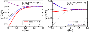
Figure 2: The OBE effective potentials for the $\Xi_{c}\bar{D}_{1}$ states with $I(J^{P})=0,1(1/2^{+},\,3/2^{+})$, where the cutoff $\Lambda$ is fixed as the typical value $1.0$ GeV.

In the following, we study the bound state solutions for the $\Xi_{c}\bar{D}_{1}$ system by solving the Schr$\ddot{\rm o}$dinger equation. First, we discuss the bound state properties of the $\Xi_{c}\bar{D}_{1}$ system by considering the $S$-$D$ wave mixing analysis, and the relevant numerical results are presented in Table 2. For the isovector $\Xi_{c}\bar{D}_{1}$ states with $J^{P}=1/2^{+}$ and $3/2^{+}$, we cannot find the bound state solutions by scanning the cutoff values $\Lambda=0.8\sim 2.5~{}{\rm GeV}$ in the $S$-$D$ wave mixing case, since the OBE effective potentials are weakly attractive for both states as illustrated in Fig. 2. For the isoscalar $\Xi_{c}\bar{D}_{1}$ states with $J^{P}=1/2^{+}$ and $3/2^{+}$, the bound state solutions can be found by choosing the cutoff values $\Lambda$ around 1.32 GeV, which is close to the reasonable range around 1.0 GeV. Thus, the isoscalar $\Xi_{c}\bar{D}_{1}$ states with $J^{P}=1/2^{+}$ and $3/2^{+}$ can be regarded as the most promising hidden-charm molecular pentaquark candidates with strangeness. Nevertheless, if we use the same cutoff value as input, there exists the same bound state properties for the isoscalar $\Xi_{c}\bar{D}_{1}$ states with $J^{P}=1/2^{+}$ and $3/2^{+}$ in the context of the $S$-$D$ wave mixing analysis, since the $\Xi_{c}\bar{D}_{1}$ system does not exist the spin-spin interaction to split into the isoscalar $\Xi_{c}\bar{D}_{1}$ bound states with $J^{P}=1/2^{+}$ and $3/2^{+}$. Thus, there exists the phenomenon of the mass degeneration for the isoscalar $\Xi_{c}\bar{D}_{1}$ bound states with $J^{P}=1/2^{+}$ and $3/2^{+}$ when adopting the same cutoff value in the $S$-$D$ wave mixing case, and such phenomenon is also found for the isoscalar $\Xi_{c}\bar{D}^{*}$ system Wang:2022mxy .

Table 2: The cutoff values dependence of the bound state solutions for the $\Xi_{c}\bar{D}_{1}$ system by considering the $S$-$D$ wave mixing case and the coupled channel case. Here, the dominant contribution channel is shown in bold font, while the units of the cutoff $\Lambda$, binding energy $E$, and root-mean-square radius $r_{{\rm RMS}}$ are $\rm{GeV}$, $\rm{MeV}$, and $\rm{fm}$, respectively.

$S$-$D$ wave mixing case
$I(J^{P})$	$\Lambda$	$E$	$r_{\rm RMS}$	P(${}^{2}\mathbb{S}_{\frac{1}{2}}/{}^{4}\mathbb{D}_{\frac{1}{2}}$)
$0(\frac{1}{2}^{+})$	1.32	$-0.27$	4.87	100.00/$o(0)$
	1.49	$-4.66$	1.58	100.00/$o(0)$
	1.65	$-12.46$	1.05	100.00/$o(0)$
$I(J^{P})$	$\Lambda$	$E$	$r_{\rm RMS}$	P(${}^{4}\mathbb{S}_{\frac{3}{2}}/{}^{2}\mathbb{D}_{\frac{3}{2}}/{}^{4}\mathbb{D}_{\frac{3}{2}}$)
$0(\frac{3}{2}^{+})$	1.32	$-0.27$	4.87	100.00/$o(0)$/$o(0)$
	1.49	$-4.66$	1.58	100.00/$o(0)$/$o(0)$
	1.65	$-12.46$	1.05	100.00/$o(0)$/$o(0)$
Coupled channel case
$I(J^{P})$	$\Lambda$	$E$	$r_{\rm RMS}$	P($\Xi_{c}\bar{D}_{1}/\Xi_{c}^{\prime}\bar{D}_{1}/\Xi_{c}^{*}\bar{D}_{1}/\Xi_{c}^{*}\bar{D}_{2}^{*}$)
$0(\frac{1}{2}^{+})$	1.04	$-0.56$	3.76	95.90/3.84/0.07/0.18
	1.07	$-4.57$	1.44	85.32/14.14/0.03/0.51
	1.09	$-10.06$	0.98	75.85/23.41/0.06/0.68
$1(\frac{1}{2}^{+})$	1.90	$-0.97$	2.75	93.47/5.24/0.08/1.21
	1.92	$-4.38$	1.27	88.00/9.64/0.13/2.24
	1.94	$-9.62$	0.84	84.19/12.69/0.16/2.97
$I(J^{P})$	$\Lambda$	$E$	$r_{\rm RMS}$	P($\Xi_{c}\bar{D}_{1}/\Xi_{c}\bar{D}_{2}^{*}/\Xi_{c}^{\prime}\bar{D}_{1}/\Xi_{c}^{\prime}\bar{D}_{2}^{*}/\Xi_{c}^{*}\bar{D}_{1}/\Xi_{c}^{*}\bar{D}_{2}^{*}$)
$0(\frac{3}{2}^{+})$	1.09	$-0.32$	4.59	97.98/0.13/0.43/0.39/0.58/0.49
	1.12	$-2.70$	1.88	91.21/1.24/1.43/1.87/1.26/3.00
	1.15	$-10.55$	0.93	69.84/6.78/2.66/6.45/0.76/13.51
$1(\frac{3}{2}^{+})$	1.71	$-0.68$	2.79	69.91/10.87/16.33/0.02/1.67/1.21
	1.72	$-4.65$	0.96	49.00/18.10/27.89/0.027/2.95/2.03
	1.73	$-9.97$	0.64	41.06/20.45/32.57/0.03/3.56/2.34

For the $\Xi_{c}\bar{D}_{1}$ system, we can further take into account the contribution of the coupled channel effect, and the obtained numerical results are given in Table 2. After including the role of the coupled channel effect, the isoscalar $\Xi_{c}\bar{D}_{1}$ states with $J^{P}=1/2^{+}$ and $3/2^{+}$ still exist the bound state solutions, while the isovector $\Xi_{c}\bar{D}_{1}$ states with $J^{P}=1/2^{+}$ and $3/2^{+}$ can form the bound states with the cutoff values restricted to be below 2.0 GeV. For the isoscalar $\Xi_{c}\bar{D}_{1}$ states with $J^{P}=1/2^{+}$ and $3/2^{+}$, the bound state solutions can be obtained by choosing the cutoff values $\Lambda$ around 1.04 GeV and 1.09 GeV, respectively, where the dominant component is the $\Xi_{c}\bar{D}_{1}$ channel. Furthermore, when taking the same cutoff value, the isoscalar $\Xi_{c}\bar{D}_{1}$ states with $J^{P}=1/2^{+}$ and $3/2^{+}$ have different bound state solutions after considering the influence of the coupled channel effect, which is similar to the case for the isoscalar $\Xi_{c}\bar{D}^{*}$ system Wang:2022mxy . We hope that the future experiments can focus on the phenomenon of the mass difference for the isoscalar $\Xi_{c}\bar{D}_{1}$ states with $J^{P}=1/2^{+}$ and $3/2^{+}$, which can test the importance of the coupled channel effect for studying the hadron-hadron interactions and the double peak hypothesis of the $P_{\psi s}^{\Lambda}(4459)$ LHCb:2020jpq existing in the $J/\psi\Lambda$ invariant mass spectrum. For the isovector $\Xi_{c}\bar{D}_{1}$ states with $J^{P}=1/2^{+}$ and $3/2^{+}$, there exist the bound state solutions when we tune the cutoff values $\Lambda$ to be around 1.90 GeV and 1.72 GeV, respectively, where both bound states have a main part of the $\Xi_{c}\bar{D}_{1}$ channel. Based on the analysis mentioned above, it is clear that the contribution of the coupled channel effect cannot be neglected when discussing the bound state properties of the $\Xi_{c}\bar{D}_{1}$ system.

By comparing the obtained bound state solutions of the isoscalar $\Xi_{c}\bar{D}_{1}$ states with $J^{P}=1/2^{+}$ and $3/2^{+}$, there is no priority for the isovector $\Xi_{c}\bar{D}_{1}$ states with $J^{P}=1/2^{+}$ and $3/2^{+}$ as the hidden-charm molecular pentaquark candidates with strangeness. Thus, we strongly suggest that the experiments should first search for the isoscalar $\Xi_{c}\bar{D}_{1}$ molecular states with $J^{P}=1/2^{+}$ and $3/2^{+}$ in future. Of course, the isovector $\Xi_{c}\bar{D}_{1}$ states with $J^{P}=1/2^{+}$ and $3/2^{+}$ as the possible candidates of the hidden-charm molecular pentaquarks with strangeness can be acceptable, since the obtained cutoff values are not especially away from the reasonable range around 1.0 GeV when appearing the isovector $\Xi_{c}\bar{D}_{1}$ bound states with $J^{P}=1/2^{+}$ and $3/2^{+}$.

Within the OBE model, the coupling constants serve as the crucial inputs to describe the interaction strengths. As a rule, we prefer to derive the coupling constants by reproducing the experimental widths with the available experimental data. In addition, we can only estimate several coupling constants by utilising various theoretical models if the pertinent experimental data are unavailable. At present, there is no experimental data available regarding the coupling constant $g_{\sigma}^{\prime\prime}$, that can be estimated using the phenomenological model in this study. However, there are various values for the coupling constant $g_{\sigma}^{\prime\prime}$ from different approaches, such as $-0.76$, $-3.40$, and $-5.21$, which are determined by the spontaneously broken chiral symmetry Wang:2019nwt , the quark model Liu:2019stu , and the correlated two-pion exchange with the pole approximation Kim:2019rud . Here, it should be noted that the $\sigma\bar{D}_{1}\bar{D}_{1}$ coupling constant is identical to the $\sigma\bar{D}^{*}\bar{D}^{*}$ coupling constant in the quark model. In the following, we discuss the bound state solutions for the isoscalar $\Xi_{c}\bar{D}_{1}$ state with $J^{P}=1/2^{+}$ by considering the uncertainties of the coupling constant $g_{\sigma}^{\prime\prime}$. In Table 3, we display the obtained bound state solutions for the isoscalar $\Xi_{c}\bar{D}_{1}$ state with $J^{P}=1/2^{+}$ by taking $g_{\sigma}^{\prime\prime}=-0.76,-3.40$, and $-5.21$. From Table 3, it can be observed that the bound state solutions for the isoscalar $\Xi_{c}\bar{D}_{1}$ state with $J^{P}=1/2^{+}$ will change, but the isoscalar $\Xi_{c}\bar{D}_{1}$ state with $J^{P}=1/2^{+}$ still can be recommended as the most promising hidden-charm molecular pentaquark candidate with strangeness when considering the uncertainties of the coupling constant $g_{\sigma}^{\prime\prime}$.

Table 3: Bound state solutions for the isoscalar $\Xi_{c}\bar{D}_{1}$ state with $J^{P}=1/2^{+}$ by taking $g_{\sigma}^{\prime\prime}=-0.76,-3.40$, and $-5.21$. The units of the cutoff $\Lambda$, binding energy $E$, and root-mean-square radius $r_{{\rm RMS}}$ are $\rm{GeV}$, $\rm{MeV}$, and $\rm{fm}$, respectively.

$g_{\sigma}^{\prime\prime}=-0.76$			$g_{\sigma}^{\prime\prime}=-3.40$			$g_{\sigma}^{\prime\prime}=-5.21$
$\Lambda$	$E$	$r_{\rm RMS}$	$\Lambda$	$E$	$r_{\rm RMS}$	$\Lambda$	$E$	$r_{\rm RMS}$
1.32	$-0.27$	4.87	0.94	$-0.28$	4.91	0.86	$-0.29$	4.87
1.49	$-4.66$	1.58	1.01	$-4.02$	1.76	0.92	$-4.74$	1.67
1.65	$-12.46$	1.05	1.08	$-11.71$	1.10	0.97	$-12.28$	1.16

III.2 $\Xi_{c}\bar{D}_{2}^{*}$ system

Similar to the $\Xi_{c}\bar{D}_{1}$ system, the $\sigma$, $\rho$, and $\omega$ exchanges provide the total effective potential for the $\Xi_{c}\bar{D}_{2}^{*}$ system within the OBE model. For the isoscalar $\Xi_{c}\bar{D}_{2}^{*}$ states with $J^{P}=3/2^{+}$ and $5/2^{+}$, the $\sigma$ and $\rho$ exchange potentials are the attractive, and the $\omega$ exchange provides the repulsive potential. For the isovector $\Xi_{c}\bar{D}_{2}^{*}$ states with $J^{P}=3/2^{+}$ and $5/2^{+}$, the attractive interaction arises from the $\sigma$ exchange, while the $\rho$ and $\omega$ exchanges give the repulsion potential. In Table 4, we collect the obtained bound state solutions for the $\Xi_{c}\bar{D}_{2}^{*}$ system by considering the $S$-$D$ wave mixing case and the coupled channel case.

Table 4: The cutoff values dependence of the bound state solutions for the $\Xi_{c}\bar{D}_{2}^{*}$ system by considering the $S$-$D$ wave mixing case and the coupled channel case. Here, the dominant contribution channel is shown in bold font, while the units of the cutoff $\Lambda$, binding energy $E$, and root-mean-square radius $r_{{\rm RMS}}$ are $\rm{GeV}$, $\rm{MeV}$, and $\rm{fm}$, respectively.

$S$-$D$ wave mixing case
$I(J^{P})$	$\Lambda$	$E$	$r_{\rm RMS}$	P(${}^{4}\mathbb{S}_{\frac{3}{2}}/{}^{4}\mathbb{D}_{\frac{3}{2}}/{}^{6}\mathbb{D}_{\frac{3}{2}}$)
$0(\frac{3}{2}^{+})$	1.32	$-0.32$	4.63	100.00/$o(0)$/$o(0)$
	1.49	$-4.89$	1.54	100.00/$o(0)$/$o(0)$
	1.65	$-12.86$	1.03	100.00/$o(0)$/$o(0)$
$I(J^{P})$	$\Lambda$	$E$	$r_{\rm RMS}$	P(${}^{6}\mathbb{S}_{\frac{5}{2}}/{}^{4}\mathbb{D}_{\frac{5}{2}}/{}^{6}\mathbb{D}_{\frac{5}{2}}$)
$0(\frac{5}{2}^{+})$	1.32	$-0.32$	4.63	100.00/$o(0)$/$o(0)$
	1.49	$-4.89$	1.54	100.00/$o(0)$/$o(0)$
	1.65	$-12.86$	1.03	100.00/$o(0)$/$o(0)$
Coupled channel case
$I(J^{P})$	$\Lambda$	$E$	$r_{\rm RMS}$	P($\Xi_{c}\bar{D}_{2}^{*}/\Xi_{c}^{\prime}\bar{D}_{1}/\Xi_{c}^{\prime}\bar{D}_{2}^{*}/\Xi_{c}^{*}\bar{D}_{1}/\Xi_{c}^{*}\bar{D}_{2}^{*}$)
$0(\frac{3}{2}^{+})$	1.06	$-0.29$	4.69	98.02/0.28/0.57/0.06/1.07
	1.10	$-3.68$	1.63	91.56/0.90/1.02/0.47/6.04
	1.13	$-10.56$	0.98	81.06/1.03/0.15/1.79/15.98
$1(\frac{3}{2}^{+})$	1.86	$-1.34$	2.14	78.06/17.92/0.28/2.17/1.56
	1.87	$-3.92$	1.19	68.33/25.96/0.38/3.19/2.14
	1.88	$-7.30$	0.85	62.02/31.19/0.44/3.88/2.47
$I(J^{P})$	$\Lambda$	$E$	$r_{\rm RMS}$	P($\Xi_{c}\bar{D}_{2}^{*}/\Xi_{c}^{\prime}\bar{D}_{2}^{*}/\Xi_{c}^{*}\bar{D}_{1}/\Xi_{c}^{*}\bar{D}_{2}^{*}$)
$0(\frac{5}{2}^{+})$	1.05	$-0.40$	4.25	97.77/0.46/0.28/1.49
	1.09	$-4.53$	1.48	91.10/1.73/1.11/6.06
	1.12	$-11.14$	0.98	84.77/2.83/1.90/10.50
$1(\frac{5}{2}^{+})$	1.58	$-0.15$	5.09	94.31/1.64/0.66/3.39
	1.60	$-5.30$	1.10	76.87/7.17/2.59/13.37
	1.61	$-9.76$	0.80	71.47/9.08/3.14/16.31

In the context of the $S$-$D$ wave mixing analysis, the bound state solutions for the isoscalar $\Xi_{c}\bar{D}_{2}^{*}$ states with $J^{P}=3/2^{+}$ and $5/2^{+}$ appear when the cutoff values $\Lambda$ are tuned larger than $1.32$ GeV, which is the reasonable cutoff value. Moreover, the probabilities for the $D$-wave channels are zero, since there does not exist the contribution of the tensor force mixing the $S$-wave and $D$-wave components in the OBE effective potentials for the $\Xi_{c}\bar{D}_{2}^{*}$ system. Based on our obtained numerical results, the isoscalar $\Xi_{c}\bar{D}_{2}^{*}$ states with $J^{P}=3/2^{+}$ and $5/2^{+}$ can be recommended as the most promising hidden-charm molecular pentaquark candidates with strangeness. Similar to the case of the isoscalar $\Xi_{c}\bar{D}_{1}$ bound states with $J^{P}=1/2^{+}$ and $3/2^{+}$, the numerical results shown in Table 4 indicate that the isoscalar $\Xi_{c}\bar{D}_{2}^{*}$ bound states with $J^{P}=3/2^{+}$ and $5/2^{+}$ also exist the phenomenon of the mass degeneration when we take the same cutoff value as input in the $S$-$D$ wave mixing case. For the isovector $\Xi_{c}\bar{D}_{2}^{*}$ states with $J^{P}=3/2^{+}$ and $5/2^{+}$, we have not found the bound state solutions when the cutoff values lie between 0.8 and 2.5 GeV. In addition, the $\Xi_{c}\bar{D}_{1}$ and $\Xi_{c}\bar{D}_{2}^{*}$ systems have the same interactions, but the binding energies of the isoscalar $\Xi_{c}\bar{D}_{2}^{*}$ states with $J^{P}=3/2^{+}$ and $5/2^{+}$ are larger than those of the isoscalar $\Xi_{c}\bar{D}_{1}$ states with $J^{P}=1/2^{+}$ and $3/2^{+}$ if we adopt the same cutoff value, since the hadrons with heavier masses are more easily form the bound states due to the relatively small kinetic terms.

Furthermore, we take into account the role of the coupled channel effect for the $\Xi_{c}\bar{D}_{2}^{*}$ system. As indicated in Table 4, the bound state solutions for the isoscalar $\Xi_{c}\bar{D}_{2}^{*}$ states with $J^{P}=3/2^{+}$ and $5/2^{+}$ can be obtained with the cutoff values $\Lambda$ above 1.06 GeV and 1.05 GeV, respectively, where the dominant channel is the $\Xi_{c}\bar{D}_{2}^{*}$ with the probability over 80%. Different from the single channel and $S$-$D$ wave mixing cases, the isoscalar $\Xi_{c}\bar{D}_{2}^{*}$ states with $J^{P}=3/2^{+}$ and $5/2^{+}$ have different bound state properties when taking the same cutoff value after including the influence of the coupled channel effect. Such a case is particularly interesting, and it is a good place to test the role of the coupled channel effect for studying the hadron-hadron interactions. Besides, our study indicates that the contribution from the coupled channel effect is crucial for the formation of the isovector $\Xi_{c}\bar{D}_{2}^{*}$ bound states with $J^{P}=3/2^{+}$ and $5/2^{+}$, and their bound state solutions can be found when the cutoff values are fixed to be larger than 1.86 GeV and 1.58 GeV, respectively. For both bound states, the $\Xi_{c}\bar{D}_{2}^{*}$ component is dominant and decreases as the cutoff parameter increases, while the contributions of other coupled channels are also important in generating both bound states.

As we can see, the isoscalar $\Xi_{c}\bar{D}_{2}^{*}$ states with $J^{P}=3/2^{+}$ and $5/2^{+}$ are expected to be the most promising hidden-charm molecular pentaquark candidates with strangeness, while the isovector $\Xi_{c}\bar{D}_{2}^{*}$ states with $J^{P}=3/2^{+}$ and $5/2^{+}$ may be the possible candidates of the hidden-charm molecular pentaquarks with strangeness.

III.3 $\Xi_{c}^{\prime}\bar{D}_{1}$ system

For the $\Xi_{c}^{\prime}\bar{D}_{1}$ system, the $\pi$ and $\eta$ exchanges also contribute to the total effective potential, except for the $\sigma$, $\rho$, and $\omega$ exchange interactions. In addition, the relevant channels for the $\Xi_{c}^{\prime}\bar{D}_{1}$ system with the same total angular momentum $J$ and parity $P$ but the different spins $S$ and orbital angular momenta $L$ can mix each other due to the existence of the tensor force operator in the OBE effective potential, which leads to the contribution of the $S$-$D$ wave mixing effect. These features are obviously different from the $\Xi_{c}\bar{D}_{1}$ and $\Xi_{c}\bar{D}_{2}^{*}$ systems. In Table 5, we give the obtained bound state properties for the $\Xi_{c}^{\prime}\bar{D}_{1}$ system by considering the single channel case, the $S$-$D$ wave mixing case, and the coupled channel case.

Table 5: The cutoff values dependence of the bound state solutions for the $\Xi_{c}^{\prime}\bar{D}_{1}$ system by considering the single channel case, the $S$-$D$ wave mixing case, and the coupled channel case. Here, the dominant contribution channel is shown in bold font, while the units of the cutoff $\Lambda$, binding energy $E$, and root-mean-square radius $r_{{\rm RMS}}$ are $\rm{GeV}$, $\rm{MeV}$, and $\rm{fm}$, respectively.

Single channel case
$I(J^{P})$	$\Lambda$	$E$	$r_{\rm RMS}$
$0(\frac{1}{2}^{+})$	0.94	$-0.34$	4.40
	1.00	$-4.81$	1.47
	1.05	$-12.80$	0.98
$0(\frac{3}{2}^{+})$	1.92	$-0.29$	4.88
	2.21	$-1.77$	2.49
	2.50	$-4.15$	1.74
$S$-$D$ wave mixing case
$I(J^{P})$	$\Lambda$	$E$	$r_{\rm RMS}$	P(${}^{2}\mathbb{S}_{\frac{1}{2}}/{}^{4}\mathbb{D}_{\frac{1}{2}}$)
$0(\frac{1}{2}^{+})$	0.93	$-0.35$	4.39	99.69/0.31
	0.99	$-4.55$	1.52	99.51/0.49
	1.04	$-12.07$	1.01	99.51/0.49
$I(J^{P})$	$\Lambda$	$E$	$r_{\rm RMS}$	P(${}^{4}\mathbb{S}_{\frac{3}{2}}/{}^{2}\mathbb{D}_{\frac{3}{2}}/{}^{4}\mathbb{D}_{\frac{3}{2}}$)
$0(\frac{3}{2}^{+})$	1.53	$-0.30$	4.87	98.78/0.20/1.02
	1.95	$-4.95$	1.65	96.78/0.50/2.72
	2.37	$-12.64$	1.15	95.81/0.65/3.54
Coupled channel case
$I(J^{P})$	$\Lambda$	$E$	$r_{\rm RMS}$	P($\Xi_{c}^{\prime}\bar{D}_{1}/\Xi_{c}^{*}\bar{D}_{1}/\Xi_{c}^{*}\bar{D}_{2}^{*}$)
$0(\frac{1}{2}^{+})$	0.91	$-0.21$	4.94	99.40/0.48/0.12
	0.96	$-4.30$	1.52	96.38/2.98/0.65
	1.00	$-12.00$	0.97	91.96/6.73/1.31
$I(J^{P})$	$\Lambda$	$E$	$r_{\rm RMS}$	P($\Xi_{c}^{\prime}\bar{D}_{1}/\Xi_{c}^{\prime}\bar{D}_{2}^{*}/\Xi_{c}^{*}\bar{D}_{1}/\Xi_{c}^{*}\bar{D}_{2}^{*}$)
$0(\frac{3}{2}^{+})$	1.07	$-3.13$	1.01	23.01/54.40/9.45/13.14
	1.08	$-7.68$	0.68	13.39/59.97/10.42/16.22
	1.09	$-12.86$	0.59	9.51/61.29/10.86/18.34
$1(\frac{3}{2}^{+})$	1.99	$-0.14$	5.08	97.58/0.09/2.09/0.25
	2.02	$-4.97$	1.13	91.25/0.33/7.53/0.89
	2.04	$-10.55$	0.77	88.95/0.43/9.49/1.13

For the isoscalar $\Xi_{c}^{\prime}\bar{D}_{1}$ state with $J^{P}=1/2^{+}$, the solutions of the bound state can be found when we set the cutoff value to be 0.96 GeV in the single channel case, and the binding energies become large with the increase of the cutoff values. If considering the $S$-$D$ wave mixing effect with channels mixing among the $|{}^{2}\mathbb{S}_{{1}/{2}}\rangle$ and $|{}^{4}\mathbb{D}_{{1}/{2}}\rangle$, we can obtain the bound state solutions for the isoscalar $\Xi_{c}^{\prime}\bar{D}_{1}$ state with $J^{P}=1/2^{+}$ when the cutoff value $\Lambda$ is fixed larger than 0.93 GeV, where the $|{}^{2}\mathbb{S}_{{1}/{2}}\rangle$ channel has the dominant contribution with the probability over 99%. In other words, the role of the $S$-$D$ wave mixing effect is tiny for the formation of this bound state. After including the coupled channel effect from the $\Xi_{c}^{\prime}\bar{D}_{1}$, $\Xi_{c}^{*}\bar{D}_{1}$, and $\Xi_{c}^{*}\bar{D}_{2}^{*}$ channels, the bound state solutions can be found when we choose the cutoff value around 0.91 GeV, where the $\Xi_{c}^{\prime}\bar{D}_{1}$ channel contribution is dominant with the probability greater than 90% and the remaining channels have small probabilities. Since the isoscalar $\Xi_{c}^{\prime}\bar{D}_{1}$ bound state with $J^{P}=1/2^{+}$ has the small binding energy and the large size with the reasonable cutoff value around 1.0 GeV, the isoscalar $\Xi_{c}^{\prime}\bar{D}_{1}$ state with $J^{P}=1/2^{+}$ can be assigned as the most promising hidden-charm molecular pentaquark candidate with strangeness.

For the isoscalar $\Xi_{c}^{\prime}\bar{D}_{1}$ state with $J^{P}=3/2^{+}$, the existence of the bound state solutions requires that the cutoff value should be at least larger than 1.92 GeV in the single channel case. After adding the contributions of the $D$-wave channels, there exists the bound state solutions with the cutoff value around 1.53 GeV for the isoscalar $\Xi_{c}^{\prime}\bar{D}_{1}$ state with $J^{P}=3/2^{+}$, where the contribution of the $S$-wave channel is over 95%. By comparing the obtained bound state solutions for the isoscalar $\Xi_{c}^{\prime}\bar{D}_{1}$ state with $J^{P}=3/2^{+}$ in the single channel and $S$-$D$ wave mixing cases, the cutoff value in the $S$-$D$ wave mixing analysis is smaller than that in the single channel analysis when obtaining the same binding energy, which means that the $S$-$D$ wave mixing effect plays the important role in generating the isoscalar $\Xi_{c}^{\prime}\bar{D}_{1}$ bound state with $J^{P}=3/2^{+}$. Furthermore, the isoscalar $\Xi_{c}^{\prime}\bar{D}_{1}$ bound state with $J^{P}=3/2^{+}$ has the small binding energy and the suitable size under the reasonable cutoff value after considering the $S$-$D$ wave mixing effect. Thus, the isoscalar $\Xi_{c}^{\prime}\bar{D}_{1}$ state with $J^{P}=3/2^{+}$ may be the promising candidate of the hidden-charm molecular pentaquark with strangeness. After that, we also discuss the bound state properties for the isoscalar $\Xi_{c}^{\prime}\bar{D}_{1}$ state with $J^{P}=3/2^{+}$ by considering the coupled channel effect, but this coupled system is dominated by the $\Xi_{c}^{\prime}\bar{D}_{2}^{*}$ channel, which results a little small size for this bound state Chen:2017xat . This can be attributed to the effective interaction of the isoscalar $\Xi_{c}^{\prime}\bar{D}_{2}^{*}$ state with $J^{P}=3/2^{+}$ is far stronger than that of the isoscalar $\Xi_{c}^{\prime}\bar{D}_{1}$ state with $J^{P}=3/2^{+}$ when we adopt the same cutoff value (see Fig. 3 for more details), and the thresholds of the $\Xi_{c}^{\prime}\bar{D}_{1}$ and $\Xi_{c}^{\prime}\bar{D}_{2}^{*}$ channels are very close with the difference is 39 MeV. As proposed in Ref. Wang:2022mxy , the cutoff values for the involved coupled channels may be different in reality, which may result in the coupled channel effect only playing the role of decorating the bound state properties for the pure state. As discussed above, when existing the related experimental information, the bound state properties of the isoscalar $\Xi_{c}^{\prime}\bar{D}_{1}$ state with $J^{P}=3/2^{+}$ deserve further studies by including the coupled channel effect and adopting different cutoff values for the involved coupled channels in future, and this approach has been used to discuss the double peak structures of the $P_{\psi s}^{\Lambda}(4459)$ under the $\Xi_{c}\bar{D}^{*}$ molecule picture in Ref. Wang:2022mxy .

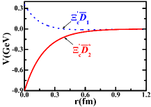
Figure 3: The OBE effective potentials for the $\Xi_{c}^{\prime}\bar{D}_{1}$ and $\Xi_{c}^{\prime}\bar{D}_{2}^{*}$ states with $I(J^{P})=0(3/2^{+})$, where the cutoff value $\Lambda$ is taken as $1.08$ GeV for an illustration.

For the isovector $\Xi_{c}^{\prime}\bar{D}_{1}$ state with $J^{P}=1/2^{+}$, the interaction is not strong enough to form the bound state even though we tune the cutoff values as high as 2.5 GeV and consider the coupled channel effect. Thus, our obtained numerical results disfavor the existence of the hidden-charm molecular pentaquark candidate with strangeness for the isovector $\Xi_{c}^{\prime}\bar{D}_{1}$ state with $J^{P}=1/2^{+}$. For the isovector $\Xi_{c}^{\prime}\bar{D}_{1}$ state with $J^{P}=3/2^{+}$, there is no bound state solutions in the single channel and the $S$-$D$ wave mixing cases by scanning the cutoff values from $0.8$ to $2.5\,{\rm GeV}$. When further adding the role of the coupled channel effect from the $\Xi_{c}^{\prime}\bar{D}_{1}$, $\Xi_{c}^{\prime}\bar{D}_{2}^{*}$, $\Xi_{c}^{*}\bar{D}_{1}$, and $\Xi_{c}^{*}\bar{D}_{2}^{*}$ channels, there exists the bound state solutions with the cutoff value $\Lambda$ slightly below 2.0 GeV, where the probability of the $\Xi_{c}^{\prime}\bar{D}_{1}$ channel is more than 88%. However, such cutoff parameter is a little away from the typical value around 1.0 GeV, which indicates that the isovector $\Xi_{c}^{\prime}\bar{D}_{1}$ state with $J^{P}=3/2^{+}$ can be treated as the potential candidate of the hidden-charm molecular pentaquark with strangeness, rather than the most promising candidate.

In the following, we discuss the tensor interactions of the $\pi$ and $\rho$ exchange potentials for the isoscalar $\Xi_{c}^{\prime}\bar{D}_{1}$ state with $J^{P}=1/2^{+}$. In Fig. 4, we present the tensor interactions of the $\pi$ and $\rho$ exchange potentials for the isoscalar $\Xi_{c}^{\prime}\bar{D}_{1}$ state with $J^{P}=1/2^{+}$. As shown in Fig. 4, the tensor interaction is optimized by the balance of the $\pi$ and $\rho$ exchange potentials for the isoscalar $\Xi_{c}^{\prime}\bar{D}_{1}$ state with $J^{P}=1/2^{+}$, which is similar to the case of the $NN$ interaction.

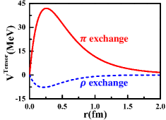
Figure 4: The tensor interactions of the $\pi$ and $\rho$ exchange potentials for the isoscalar $\Xi_{c}^{\prime}\bar{D}_{1}$ state with $J^{P}=1/2^{+}$, where the cutoff $\Lambda$ is fixed as the typical value $1.0$ GeV.

III.4 $\Xi_{c}^{\prime}\bar{D}_{2}^{*}$ system

For the $S$-wave $\Xi_{c}^{\prime}\bar{D}_{2}^{*}$ system, the total effective potential arises from the $\sigma$, $\pi$, $\eta$, $\rho$, and $\omega$ exchanges within the OBE model, while the allowed quantum numbers contain $I(J^{P})=0({3}/{2}^{+})$, $0({5}/{2}^{+})$, $1({3}/{2}^{+})$, and $1({5}/{2}^{+})$. In Table 6, we collect the obtained bound state solutions for the $\Xi_{c}^{\prime}\bar{D}_{2}^{*}$ system by considering the single channel case, the $S$-$D$ wave mixing case, and the coupled channel case.

Table 6: The cutoff values dependence of the bound state solutions for the $\Xi_{c}^{\prime}\bar{D}_{2}^{*}$ system by considering the single channel case, the $S$-$D$ wave mixing case, and the coupled channel case. Here, the dominant contribution channel is shown in bold font, while the units of the cutoff $\Lambda$, binding energy $E$, and root-mean-square radius $r_{{\rm RMS}}$ are $\rm{GeV}$, $\rm{MeV}$, and $\rm{fm}$, respectively.

Single channel case
$I(J^{P})$	$\Lambda$	$E$	$r_{\rm RMS}$
$0(\frac{3}{2}^{+})$	0.96	$-0.29$	4.59
	1.02	$-4.44$	1.52
	1.08	$-13.78$	0.95
$0(\frac{5}{2}^{+})$	1.99	$-0.28$	4.92
	2.26	$-1.57$	2.63
	2.50	$-3.35$	1.91
$1(\frac{5}{2}^{+})$	2.38	$-0.34$	4.04
	2.41	$-5.02$	1.12
	2.43	$-10.00$	0.78
$S$-$D$ wave mixing case
$I(J^{P})$	$\Lambda$	$E$	$r_{\rm RMS}$	P(${}^{4}\mathbb{S}_{\frac{3}{2}}/{}^{4}\mathbb{D}_{\frac{3}{2}}/{}^{6}\mathbb{D}_{\frac{3}{2}}$)
$0(\frac{3}{2}^{+})$	0.94	$-0.27$	4.73	99.49/0.07/0.43
	1.00	$-3.88$	1.64	99.11/0.13/0.76
	1.06	$-12.18$	1.02	99.11/0.13/0.76
$I(J^{P})$	$\Lambda$	$E$	$r_{\rm RMS}$	P(${}^{6}\mathbb{S}_{\frac{5}{2}}/{}^{4}\mathbb{D}_{\frac{5}{2}}/{}^{6}\mathbb{D}_{\frac{5}{2}}$)
$0(\frac{5}{2}^{+})$	1.56	$-0.31$	4.83	98.63/0.41/0.96
	1.99	$-4.91$	1.67	96.34/1.07/2.59
	2.42	$-12.89$	1.15	95.19/1.39/3.43
$1(\frac{5}{2}^{+})$	2.33	$-0.25$	4.44	99.79/0.06/0.15
	2.36	$-4.52$	1.19	99.43/1.15/0.42
	2.38	$-9.20$	0.84	99.29/0.19/0.52
Coupled channel case
$I(J^{P})$	$\Lambda$	$E$	$r_{\rm RMS}$	P($\Xi_{c}^{\prime}\bar{D}_{2}^{*}/\Xi_{c}^{*}\bar{D}_{1}/\Xi_{c}^{*}\bar{D}_{2}^{*}$)
$0(\frac{3}{2}^{+})$	0.93	$-0.51$	3.81	98.44/0.33/1.23
	0.97	$-4.27$	1.50	93.92/1.39/4.69
	1.01	$-12.44$	0.94	86.77/3.09/10.14
$0(\frac{5}{2}^{+})$	1.26	$-0.36$	4.33	92.19/1.76/6.05
	1.30	$-4.88$	1.29	67.14/7.07/25.79
	1.33	$-11.67$	0.83	52.74/9.56/37.70
$1(\frac{5}{2}^{+})$	1.88	$-0.35$	4.02	96.29/1.71/2.00
	1.90	$-3.11$	1.43	91.23/4.36/4.41
	1.92	$-7.68$	0.91	88.01/6.27/5.73

In the single channel case, the OBE effective potentials are sufficient to form the $\Xi_{c}^{\prime}\bar{D}_{2}^{*}$ bound states with $I(J^{P})=0({3}/{2}^{+})$, $0({5}/{2}^{+})$, and $1({5}/{2}^{+})$ when the cutoff values are taken to be around 0.96, 1.99, and 2.38 GeV, respectively. However, we fail to find the bound state solutions for the $\Xi_{c}^{\prime}\bar{D}_{2}^{*}$ state with $I(J^{P})=1({3}/{2}^{+})$ when the cutoff values $\Lambda$ are scanned from 0.8 to 2.5 GeV. In the following, we continue to discuss the bound state properties for the $\Xi_{c}^{\prime}\bar{D}_{2}^{*}$ system by considering the $S$-$D$ wave mixing effect and the coupled channel effect.

For the $\Xi_{c}^{\prime}\bar{D}_{2}^{*}$ state with $I(J^{P})=0({3}/{2}^{+})$, we can consider the $S$-$D$ wave mixing effect from the $|{}^{4}\mathbb{S}_{{3}/{2}}\rangle$, $|{}^{4}\mathbb{D}_{{3}/{2}}\rangle$, and $|{}^{6}\mathbb{D}_{{3}/{2}}\rangle$ channels, and there exists the bound state solutions when the cutoff value $\Lambda$ should be at least 0.94 GeV, where the $|{}^{4}\mathbb{S}_{{3}/{2}}\rangle$ is the dominant channel with the probability over 99%. However, when the $S$-$D$ wave mixing effect is included, the conclusion of the absence of the bound state solutions does not change for the $\Xi_{c}^{\prime}\bar{D}_{2}^{*}$ state with $I(J^{P})=1({3}/{2}^{+})$ if we fix the cutoff values $\Lambda$ smaller than 2.5 GeV. After adding the contribution of the $S$-$D$ wave mixing effect among the $|{}^{6}\mathbb{S}_{{5}/{2}}\rangle$, $|{}^{4}\mathbb{D}_{{5}/{2}}\rangle$, and $|{}^{6}\mathbb{D}_{{5}/{2}}\rangle$ channels, the $\Xi_{c}^{\prime}\bar{D}_{2}^{*}$ states with $I(J^{P})=0({5}/{2}^{+})$ and $1({5}/{2}^{+})$ have the bound state solutions when the cutoff values $\Lambda$ are larger than 1.56 GeV and 2.33 GeV, respectively. Compared to the obtained bound state solutions in the single channel case, the $S$-$D$ wave mixing effect plays the important role for forming the $\Xi_{c}^{\prime}\bar{D}_{2}^{*}$ bound state with $I(J^{P})=0({5}/{2}^{+})$. Nevertheless, the bound state properties of the $\Xi_{c}^{\prime}\bar{D}_{2}^{*}$ states with $I(J^{P})=0({3}/{2}^{+})$ and $1({5}/{2}^{+})$ change slightly after considering the role of the $S$-$D$ wave mixing effect, and the total probability of the $D$-wave channels is less than 1%, which provides the negligible contributions.

Meanwhile, we consider the influence of the coupled channel effect from the $\Xi_{c}^{\prime}\bar{D}_{2}^{*}$, $\Xi_{c}^{*}\bar{D}_{1}$, and $\Xi_{c}^{*}\bar{D}_{2}^{*}$ channels for the $\Xi_{c}^{\prime}\bar{D}_{2}^{*}$ system. For the $\Xi_{c}^{\prime}\bar{D}_{2}^{*}$ state with $I(J^{P})=0({3}/{2}^{+})$, the bound state solutions can be found when the cutoff value is fixed to be larger than 0.93 GeV, where the $\Xi_{c}^{\prime}\bar{D}_{2}^{*}$ channel provides the dominant contribution with the probability over 86%. Moreover, the coupled channel effect plays the important role for forming the $\Xi_{c}^{\prime}\bar{D}_{2}^{*}$ bound states with $I(J^{P})=0({5}/{2}^{+})$ and $1({5}/{2}^{+})$, and their bound state solutions appear when the cutoff values are larger than 1.26 GeV and 1.88 GeV, respectively. Correspondingly, the $\Xi_{c}^{\prime}\bar{D}_{2}^{*}$ is the dominant channel, and the contributions of other coupled channels increase with the cutoff values. For the $\Xi_{c}^{\prime}\bar{D}_{2}^{*}$ state with $I(J^{P})=1({3}/{2}^{+})$, we also cannot find the bound state solutions corresponding to the cutoff values $\Lambda=0.8\sim 2.5\,{\rm GeV}$ even if including the coupled channel effect.

According to our quantitative analysis, the $\Xi_{c}^{\prime}\bar{D}_{2}^{*}$ states with $I(J^{P})=0({3}/{2}^{+})$ and $0({5}/{2}^{+})$ can be recommended as the most promising hidden-charm molecular pentaquark candidates with strangeness, the $\Xi_{c}^{\prime}\bar{D}_{2}^{*}$ state with $I(J^{P})=1({5}/{2}^{+})$ may be the possible candidate of the hidden-charm molecular pentaquark with strangeness, and the $\Xi_{c}^{\prime}\bar{D}_{2}^{*}$ state with $I(J^{P})=1({3}/{2}^{+})$ is not considered as the hidden-charm molecular pentaquark candidate with strangeness.

III.5 $\Xi_{c}^{*}\bar{D}_{1}$ system

For the $S$-wave $\Xi_{c}^{*}\bar{D}_{1}$ system, the $\sigma$, $\pi$, $\eta$, $\rho$, and $\omega$ exchanges contribute to the total effective potential, while the allowed quantum numbers are $I(J^{P})=0({1}/{2}^{+})$, $0({3}/{2}^{+})$, $0({5}/{2}^{+})$, $1({1}/{2}^{+})$, $1({3}/{2}^{+})$, and $1({5}/{2}^{+})$. Here, we perform the comprehensive and systematic analysis of the bound state properties for the $\Xi_{c}^{*}\bar{D}_{1}$ system by conducting the single channel analysis, the $S$-$D$ wave mixing analysis, and the coupled channel analysis.

In Table 7, we present the obtained bound state properties for the $\Xi_{c}^{*}\bar{D}_{1}$ system by considering the single channel case and the $S$-$D$ wave mixing case. From the numerical results listed in Table 7, the $\Xi_{c}^{*}\bar{D}_{1}$ states with $I(J^{P})=0({1}/{2}^{+})$ and $0({3}/{2}^{+})$ exist the bound state solutions when we choose the cutoff values about 0.88 GeV and 1.08 GeV in the single channel analysis, respectively. As the cutoff values are increased, both bound states bind deeper and deeper. When further adding the contributions from the $D$-wave channels, the bound state solutions also appear for the $\Xi_{c}^{*}\bar{D}_{1}$ states with $I(J^{P})=0({1}/{2}^{+})$ and $0({3}/{2}^{+})$ with the cutoff values around 0.86 GeV and 1.04 GeV, respectively, where the $S$-wave percentage is more than 98% and plays the important role to generate both bound states. Compared to the obtained numerical results in the single channel case, the bound state properties for the $\Xi_{c}^{*}\bar{D}_{1}$ states with $I(J^{P})=0({1}/{2}^{+})$ and $0({3}/{2}^{+})$ do not change too much after including the $S$-$D$ wave mixing effect. Moreover, the $\Xi_{c}^{*}\bar{D}_{1}$ states with $I(J^{P})=0({5}/{2}^{+})$ and $1({5}/{2}^{+})$ can form the bound states when the cutoff values $\Lambda$ are set to be around 2.06 GeV in the context of the single channel analysis. After including the $S$-$D$ wave mixing effect among the $|{}^{6}\mathbb{S}_{{5}/{2}}\rangle$, $|{}^{2}\mathbb{D}_{{5}/{2}}\rangle$, $|{}^{4}\mathbb{D}_{{5}/{2}}\rangle$, and $|{}^{6}\mathbb{D}_{{5}/{2}}\rangle$ channels, the bound state properties for the $\Xi_{c}^{*}\bar{D}_{1}$ states with $I(J^{P})=0({5}/{2}^{+})$ and $1({5}/{2}^{+})$ will change, and we can obtain their bound state solutions when the cutoff values $\Lambda$ are lowered down 1.56 GeV and 2.04 GeV, respectively. The contributions of the $D$-wave channels are quite small, and the probability of the dominant $S$-wave channel is over 99% for the $\Xi_{c}^{*}\bar{D}_{1}$ bound state with $I(J^{P})=1({5}/{2}^{+})$. Comparing the obtained numerical results, the $S$-$D$ wave mixing effect is salient in generating the $\Xi_{c}^{*}\bar{D}_{1}$ bound state with $I(J^{P})=0({5}/{2}^{+})$, and the contribution of the $|{}^{6}\mathbb{D}_{{5}/{2}}\rangle$ channel is important, except for the $|{}^{6}\mathbb{S}_{{5}/{2}}\rangle$ channel. Unfortunately, there does not exist the bound state solutions for the $\Xi_{c}^{*}\bar{D}_{1}$ states with $I(J^{P})=1({1}/{2}^{+})$ and $1({3}/{2}^{+})$ when the cutoff values are chosen between 0.8 to 2.5 GeV and the $S$-$D$ wave mixing effect is included.

Table 7: The cutoff values dependence of the bound state solutions for the $\Xi_{c}^{*}\bar{D}_{1}$ system by considering the single channel case and the $S$-$D$ wave mixing case. Here, the dominant contribution channel is shown in bold font, while the units of the cutoff $\Lambda$, binding energy $E$, and root-mean-square radius $r_{{\rm RMS}}$ are $\rm{GeV}$, $\rm{MeV}$, and $\rm{fm}$, respectively.

Single channel case
$I(J^{P})$	$\Lambda$	$E$	$r_{\rm RMS}$
$0(\frac{1}{2}^{+})$	0.88	$-0.28$	4.61
	0.94	$-4.78$	1.46
	0.99	$-13.33$	0.96
$0(\frac{3}{2}^{+})$	1.08	$-0.37$	4.34
	1.15	$-4.22$	1.57
	1.22	$-12.31$	1.00
$0(\frac{5}{2}^{+})$	2.06	$-0.28$	4.95
	2.28	$-1.26$	2.91
	2.50	$-2.81$	2.07
$1(\frac{5}{2}^{+})$	2.06	$-0.41$	3.81
	2.09	$-4.66$	1.19
	2.11	$-9.22$	0.84
$S$-$D$ wave mixing case
$I(J^{P})$	$\Lambda$	$E$	$r_{\rm RMS}$	P(${}^{2}\mathbb{S}_{\frac{1}{2}}/{}^{4}\mathbb{D}_{\frac{1}{2}}/{}^{6}\mathbb{D}_{\frac{1}{2}}$)
$0(\frac{1}{2}^{+})$	0.86	$-0.26$	4.75	99.46/0.32/0.21
	0.92	$-4.06$	1.60	99.07/0.57/0.36
	0.98	$-13.47$	0.98	99.09/0.56/0.35
$I(J^{P})$	$\Lambda$	$E$	$r_{\rm RMS}$	P(${}^{4}\mathbb{S}_{\frac{3}{2}}/{}^{2}\mathbb{D}_{\frac{3}{2}}/{}^{4}\mathbb{D}_{\frac{3}{2}}/{}^{6}\mathbb{D}_{\frac{3}{2}}$)
$0(\frac{3}{2}^{+})$	1.04	$-0.36$	4.41	99.16/0.23/0.55/0.06
	1.12	$-4.52$	1.56	98.48/0.42/0.99/0.11
	1.19	$-12.23$	1.03	98.38/0.45/1.05/0.12
$I(J^{P})$	$\Lambda$	$E$	$r_{\rm RMS}$	P(${}^{6}\mathbb{S}_{\frac{5}{2}}/{}^{2}\mathbb{D}_{\frac{5}{2}}/{}^{4}\mathbb{D}_{\frac{5}{2}}/{}^{6}\mathbb{D}_{\frac{5}{2}}$)
$0(\frac{5}{2}^{+})$	1.56	$-0.29$	4.95	98.38/0.93/0.05/1.48
	1.98	$-4.70$	1.72	95.53/0.23/0.13/4.12
	2.40	$-12.77$	1.18	94.03/0.29/0.17/5.51
$1(\frac{5}{2}^{+})$	2.04	$-0.89$	2.75	99.80/0.01/0.01/0.18
	2.06	$-3.75$	1.33	99.67/0.02/0.01/0.30
	2.08	$-8.00$	0.91	99.58/0.03/0.01/0.38

After that, we also study the bound state properties for the $\Xi_{c}^{*}\bar{D}_{1}$ system by adding the role of the coupled channel effect from the $\Xi_{c}^{*}\bar{D}_{1}$ and $\Xi_{c}^{*}\bar{D}_{2}^{*}$ channels, and the relevant numerical results are collected in Table 8. The $\Xi_{c}^{*}\bar{D}_{1}$ states with $I(J^{P})=0({1}/{2}^{+})$ and $0({3}/{2}^{+})$ exist the small binding energies and the suitable sizes with the cutoff values around 0.90 GeV and 1.05 GeV, respectively, where the $\Xi_{c}^{*}\bar{D}_{1}$ channel has the dominant contribution. In addition, the $\Xi_{c}^{*}\bar{D}_{2}^{*}$ channel is important for the formation of the $\Xi_{c}^{*}\bar{D}_{1}$ bound state with $I(J^{P})=0({3}/{2}^{+})$, and whose contribution is over 30% when the corresponding binding energy increases to be $-12\,{\rm MeV}$. For the $\Xi_{c}^{*}\bar{D}_{1}$ state with $I(J^{P})=0({5}/{2}^{+})$, we can obtain the bound state solutions when the cutoff value is taken to be larger than 1.42 GeV, which is the mixture state formed by the $\Xi_{c}^{*}\bar{D}_{1}$ and $\Xi_{c}^{*}\bar{D}_{2}^{*}$ channels. For the $\Xi_{c}^{*}\bar{D}_{1}$ state with $I(J^{P})=1({5}/{2}^{+})$, there exists the bound state solutions when the cutoff value is tuned larger than 1.86 GeV, where the probability of the $\Xi_{c}^{*}\bar{D}_{1}$ channel is over 93%. After considering the contribution of the coupled channel effect, the bound state solutions of the $\Xi_{c}^{*}\bar{D}_{1}$ states with $I(J^{P})=1({1}/{2}^{+})$ and $1({3}/{2}^{+})$ still disappear when the cutoff values change from 0.8 to 2.5 GeV.

Table 8: The cutoff values dependence of the bound state solutions for the $\Xi_{c}^{*}\bar{D}_{1}$ system when the coupled channel effect is considered. Here, the dominant contribution channel is shown in bold font, while the units of the cutoff $\Lambda$, binding energy $E$, and root-mean-square radius $r_{{\rm RMS}}$ are $\rm{GeV}$, $\rm{MeV}$, and $\rm{fm}$, respectively.

$I(J^{P})$	$\Lambda$	$E$	$r_{\rm RMS}$	P($\Xi_{c}^{*}\bar{D}_{1}/\Xi_{c}^{*}\bar{D}_{2}^{*}$)
$0(\frac{1}{2}^{+})$	0.88	$-0.51$	3.80	99.53/0.47
	0.93	$-4.75$	1.45	97.63/2.37
	0.97	$-11.89$	0.98	94.39/5.61
$0(\frac{3}{2}^{+})$	1.02	$-0.52$	3.77	95.89/4.11
	1.06	$-4.82$	1.36	82.40/17.60
	1.09	$-11.39$	0.91	69.78/30.22
$0(\frac{5}{2}^{+})$	1.42	$-0.23$	4.88	91.01/8.99
	1.46	$-2.89$	1.59	62.21/37.79
	1.50	$-8.48$	0.90	41.36/58.64
$1(\frac{5}{2}^{+})$	1.86	$-0.37$	3.98	97.90/2.10
	1.89	$-4.68$	1.18	94.51/5.49
	1.91	$-9.41$	0.84	93.17/6.83

To summarize, our obtained numerical results indicate that the $\Xi_{c}^{*}\bar{D}_{1}$ states with $I(J^{P})=0({1}/{2}^{+})$, $0({3}/{2}^{+})$, and $0({5}/{2}^{+})$ are favored to be the most promising hidden-charm molecular pentaquark candidates with strangeness since they have the small binding energies and the suitable sizes under the reasonable cutoff values, the $\Xi_{c}^{*}\bar{D}_{1}$ state with $I(J^{P})=1({5}/{2}^{+})$ may be viewed as the possible candidate of the hidden-charm molecular pentaquark with strangeness, while the $\Xi_{c}^{*}\bar{D}_{1}$ states with $I(J^{P})=1({1}/{2}^{+})$ and $1({3}/{2}^{+})$ as the hidden-charm molecular pentaquark candidates with strangeness can be excluded.

III.6 $\Xi_{c}^{*}\bar{D}_{2}^{*}$ system

For the $S$-wave $\Xi_{c}^{*}\bar{D}_{2}^{*}$ system, there exists the $\sigma$, $\pi$, $\eta$, $\rho$, and $\omega$ exchange interactions within the OBE model, and the allowed quantum numbers are more abundant, which include $I(J^{P})=0({1}/{2}^{+})$, $0({3}/{2}^{+})$, $0({5}/{2}^{+})$, $0({7}/{2}^{+})$, $1({1}/{2}^{+})$, $1({3}/{2}^{+})$, $1({5}/{2}^{+})$, and $1({7}/{2}^{+})$. In Table 9, the obtained bound state solutions for the $\Xi_{c}^{*}\bar{D}_{2}^{*}$ system by considering the single channel case and the $S$-$D$ wave mixing case are presented.

Table 9: The cutoff values dependence of the bound state solutions for the $\Xi_{c}^{*}\bar{D}_{2}^{*}$ system by considering the single channel case and the $S$-$D$ wave mixing case. Here, the dominant contribution channel is shown in bold font, while the units of the cutoff $\Lambda$, binding energy $E$, and root-mean-square radius $r_{{\rm RMS}}$ are $\rm{GeV}$, $\rm{MeV}$, and $\rm{fm}$, respectively.

Single channel case
$I(J^{P})$	$\Lambda$	$E$	$r_{\rm RMS}$
$0(\frac{1}{2}^{+})$	0.86	$-0.36$	4.25
	0.92	$-5.08$	1.42
	0.97	$-13.97$	0.94
$0(\frac{3}{2}^{+})$	0.96	$-0.42$	4.11
	1.02	$-4.88$	1.45
	1.07	$-12.57$	0.98
$0(\frac{5}{2}^{+})$	1.23	$-0.22$	5.00
	1.35	$-4.23$	1.59
	1.47	$-12.72$	1.00
$0(\frac{7}{2}^{+})$	2.08	$-0.27$	4.99
	2.29	$-1.22$	2.95
	2.50	$-2.76$	2.10
$1(\frac{7}{2}^{+})$	1.84	$-0.61$	3.27
	1.87	$-4.73$	1.20
	1.89	$-9.07$	0.87
$S$-$D$ wave mixing case
$I(J^{P})$	$\Lambda$	$E$	$r_{\rm RMS}$	P(${}^{2}\mathbb{S}_{\frac{1}{2}}/{}^{4}\mathbb{D}_{\frac{1}{2}}/{}^{6}\mathbb{D}_{\frac{1}{2}}$)
$0(\frac{1}{2}^{+})$	0.84	$-0.46$	3.98	99.23/0.39/0.38
	0.90	$-4.63$	1.52	98.83/0.60/0.57
	0.95	$-12.42$	1.01	98.84/0.60/0.56
$I(J^{P})$	$\Lambda$	$E$	$r_{\rm RMS}$	P(${}^{4}\mathbb{S}_{\frac{3}{2}}/{}^{2}\mathbb{D}_{\frac{3}{2}}/{}^{4}\mathbb{D}_{\frac{3}{2}}/{}^{6}\mathbb{D}_{\frac{3}{2}}/{}^{8}\mathbb{D}_{\frac{3}{2}}$)
$0(\frac{3}{2}^{+})$	0.93	$-0.39$	4.26	99.16/0.22/0.39/0.08/0.15
	0.99	$-4.10$	1.61	98.62/0.37/0.64/0.13/0.24
	1.05	$-12.33$	1.02	98.58/0.39/0.66/0.13/0.24
$I(J^{P})$	$\Lambda$	$E$	$r_{\rm RMS}$	P(${}^{6}\mathbb{S}_{\frac{5}{2}}/{}^{2}\mathbb{D}_{\frac{5}{2}}/{}^{4}\mathbb{D}_{\frac{5}{2}}/{}^{6}\mathbb{D}_{\frac{5}{2}}/{}^{8}\mathbb{D}_{\frac{5}{2}}$)
$0(\frac{5}{2}^{+})$	1.15	$-0.32$	4.61	98.86/0.16/0.06/0.89/0.03
	1.27	$-4.44$	1.61	97.65/0.34/0.13/1.83/0.05
	1.39	$-13.04$	1.04	97.31/0.40/0.15/2.08/0.06
$I(J^{P})$	$\Lambda$	$E$	$r_{\rm RMS}$	P(${}^{8}\mathbb{S}_{\frac{7}{2}}/{}^{4}\mathbb{D}_{\frac{7}{2}}/{}^{6}\mathbb{D}_{\frac{7}{2}}/{}^{8}\mathbb{D}_{\frac{7}{2}}$)
$0(\frac{7}{2}^{+})$	1.57	$-0.31$	4.84	98.10/0.08/0.02/1.79
	1.96	$-4.74$	1.73	94.84/0.19/0.06/4.92
	2.38	$-12.79$	1.19	93.11/0.23/0.08/6.59
$1(\frac{7}{2}^{+})$	1.83	$-0.80$	2.92	99.89/0.01/$o(0)$/0.10
	1.86	$-5.17$	1.15	99.81/0.01/$o(0)$/0.18
	1.89	$-9.68$	0.85	99.76/0.01/$o(0)$/0.23

In the single channel analysis, the $\Xi_{c}^{*}\bar{D}_{2}^{*}$ states with $I(J^{P})=0({1}/{2}^{+})$, $0({3}/{2}^{+})$, and $0({5}/{2}^{+})$ can be bound together to form the bound states when we set the cutoff values to be around 0.86 GeV, 0.96 GeV, and 1.23 GeV, respectively, which are the reasonable cutoff values. For the $\Xi_{c}^{*}\bar{D}_{2}^{*}$ states with $I(J^{P})=0({7}/{2}^{+})$ and $1({7}/{2}^{+})$, there exist the bound state solutions when the cutoff values are taken to be around 2.08 and 1.84 GeV, respectively. For the $\Xi_{c}^{*}\bar{D}_{2}^{*}$ states with $I(J^{P})=1({1}/{2}^{+})$, $1({3}/{2}^{+})$, and $1({5}/{2}^{+})$, the bound state solutions cannot be found if we fix the cutoff values between 0.8 to 2.5 GeV.

Now we further take into account the role of the $S$-$D$ wave mixing effect for the $\Xi_{c}^{*}\bar{D}_{2}^{*}$ system. For the $\Xi_{c}^{*}\bar{D}_{2}^{*}$ states with $I(J^{P})=0({1}/{2}^{+})$, $0({3}/{2}^{+})$, $0({5}/{2}^{+})$, and $1({7}/{2}^{+})$, the $S$-$D$ wave mixing effect plays the positive but minor role for the formation of these bound states, where the contribution of the dominant $S$-wave channel is over 97%. However, the role of the tensor force from the $S$-$D$ wave mixing effect plays the important role in generating the $\Xi_{c}^{*}\bar{D}_{2}^{*}$ bound state with $I(J^{P})=0({7}/{2}^{+})$, and the corresponding bound state solutions can be obtained when we tune the cutoff value to be around 1.57 GeV. In addition, we still cannot find the bound state solutions for the $\Xi_{c}^{*}\bar{D}_{2}^{*}$ states with $I(J^{P})=1({1}/{2}^{+})$, $1({3}/{2}^{+})$, and $1({5}/{2}^{+})$ when the cutoff values are chosen between 0.8 to 2.5 GeV and the role of the $S$-$D$ wave mixing effect is introduced.

In short summary, the $\Xi_{c}^{*}\bar{D}_{2}^{*}$ states with $I(J^{P})=0({1}/{2}^{+})$, $0({3}/{2}^{+})$, $0({5}/{2}^{+})$, and $0({7}/{2}^{+})$ can be considered as the prime hidden-charm molecular pentaquark candidates with strangeness, and the $\Xi_{c}^{*}\bar{D}_{2}^{*}$ state with $I(J^{P})=1({7}/{2}^{+})$ may be the potential candidate of the hidden-charm molecular pentaquark with strangeness. In addition, our quantitative analysis does not support the $\Xi_{c}^{*}\bar{D}_{2}^{*}$ states with $I(J^{P})=1({1}/{2}^{+})$, $1({3}/{2}^{+})$, and $1({5}/{2}^{+})$ as the hidden-charm molecular pentaquark candidates with strangeness.

IV Discussions and conclusions

Since 2003, numerous exotic hadron states have been reported by various experiments, sparking the interest in exploring these exotic hadrons and establishing them as a research frontier within the hadron physics. Notably, in 2019, LHCb announced the discoveries of the $P_{\psi}^{N}(4312)$, $P_{\psi}^{N}(4440)$, and $P_{\psi}^{N}(4457)$ states, providing robust experimental evidence supporting the existence of the hidden-charm baryon-meson molecular pentaquark states. This progress has fueled our enthusiasm for constructing the family of the hidden-charm molecular pentaquarks. Inspired by the discoveries of the $P_{\psi s}^{\Lambda}(4459)$ and $P_{\psi s}^{\Lambda}(4338)$ as the potential $\Xi_{c}\bar{D}^{(*)}$ molecules, we have undertaken an investigation of the interactions between the charmed baryons $\Xi_{c}^{(\prime,*)}$ and the anticharmed mesons $\bar{D}_{1}/\bar{D}_{2}^{*}$. This work aims to explore a novel class of molecular $P_{\psi s}^{\Lambda/\Sigma}$ pentaquark candidates, which are composed of the charmed baryons $\Xi_{c}^{(\prime,*)}$ and the anticharmed mesons $\bar{D}_{1}/\bar{D}_{2}^{*}$ and possess masses ranging from approximately $4.87$ to $5.10$ GeV. Through our study, we anticipate predicting the existence of these intriguing pentaquark states.

In our concrete calculations, we have determined the effective potentials of the $\Xi_{c}^{(\prime,*)}\bar{D}_{1}/\Xi_{c}^{(\prime,*)}\bar{D}_{2}^{*}$ systems using the OBE model. These potentials incorporate the contributions from the exchange of the $\sigma$, $\pi$, $\eta$, $\rho$, and $\omega$ particles. Furthermore, we have taken into account both the $S$-$D$ wave mixing effect and the coupled channel effect. By solving the coupled channel Schr$\ddot{\rm o}$dinger equation, we have obtained the bound state properties of the discussed systems. Based on these obtained results, we propose that the following states can be considered as the most promising molecular $P_{\psi s}^{\Lambda}$ pentaquark candidates: the $\Xi_{c}\bar{D}_{1}$ states with $I(J^{P})=0({1}/{2}^{+},\,{3}/{2}^{+})$, the $\Xi_{c}\bar{D}_{2}^{*}$ states with $I(J^{P})=0({3}/{2}^{+},\,{5}/{2}^{+})$, the $\Xi_{c}^{\prime}\bar{D}_{1}$ states with $I(J^{P})=0({1}/{2}^{+},\,{3}/{2}^{+})$, the $\Xi_{c}^{\prime}\bar{D}_{2}^{*}$ states with $I(J^{P})=0({3}/{2}^{+},\,{5}/{2}^{+})$, the $\Xi_{c}^{*}\bar{D}_{1}$ states with $I(J^{P})=0({1}/{2}^{+},\,{3}/{2}^{+},\,{5}/{2}^{+})$, and the $\Xi_{c}^{*}\bar{D}_{2}^{*}$ states with $I(J^{P})=0({1}/{2}^{+},\,{3}/{2}^{+},\,{5}/{2}^{+},\,{7}/{2}^{+})$. These findings align with the conclusions drawn in Ref. Dong:2021juy and are depicted in Fig. 5. Meanwhile, the $\Xi_{c}\bar{D}_{1}$ states with $I(J^{P})=1({1}/{2}^{+},\,{3}/{2}^{+})$, the $\Xi_{c}\bar{D}_{2}^{*}$ states with $I(J^{P})=1({3}/{2}^{+},\,{5}/{2}^{+})$, the $\Xi_{c}^{\prime}\bar{D}_{1}$ state with $I(J^{P})=1({3}/{2}^{+})$, the $\Xi_{c}^{\prime}\bar{D}_{2}^{*}$ state with $I(J^{P})=1({5}/{2}^{+})$, the $\Xi_{c}^{*}\bar{D}_{1}$ state with $I(J^{P})=1({5}/{2}^{+})$, and the $\Xi_{c}^{*}\bar{D}_{2}^{*}$ state with $I(J^{P})=1({7}/{2}^{+})$ may serve as the potential molecular $P_{\psi s}^{\Sigma}$ pentaquark candidates. However, the remaining states can be excluded as the hidden-charm molecular pentaquark candidates with strangeness. It is noteworthy that the $S$-$D$ mixing effect and the coupled channel effect are crucial for the formation of several hidden-charm molecular pentaquark candidates with strangeness. Notably, the spectroscopic behavior of the isoscalar $\Xi_{c}\bar{D}_{1}$ and $\Xi_{c}\bar{D}_{2}^{*}$ systems resembles that of the isoscalar $\Xi_{c}\bar{D}^{*}$ system Wang:2022mxy , which can split into two distinct states due to the influence of the coupled channel effect.

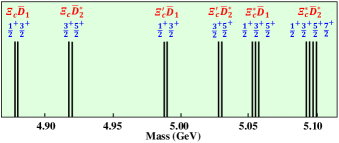
Figure 5: The characteristic spectrum of the most promising molecular $P_{\psi s}^{\Lambda}$ pentaquark candidates for the $\Xi_{c}^{(\prime,*)}\bar{D}_{1}/\Xi_{c}^{(\prime,*)}\bar{D}_{2}^{*}$ systems.

It is very intriguing and important to search for these predicted hidden-charm molecular pentaquark candidates with strangeness experimentally, which can be detected in their allowed two-body strong decay channels. The two-body strong decay final states of our predicted most promising molecular $P_{\psi s}^{\Lambda}$ pentaquark candidates contain the baryon $\Lambda$ plus the charmonium state, the baryon $\Lambda_{c}$ plus the meson $\bar{D}_{s}$, the baryon $\Xi_{c}$ plus the meson $\bar{D}$, and so on. Furthermore, the two-body strong decay channels of our predicted potential molecular $P_{\psi s}^{\Sigma}$ pentaquark candidates include the baryon $\Sigma$ plus the charmonium state, the baryon $\Sigma_{c}$ plus the meson $\bar{D}_{s}$, the baryon $\Xi_{c}$ plus the meson $\bar{D}$, and so on. Here, the baryons and mesons in these final states stand for either the ground states or the excited states. These possible two-body strong decay information can give the crucial information to detect our predicted hidden-charm molecular pentaquark candidates with strangeness in future experiments, specifically focusing on the two-body hidden-charm strong decay channels.

With the higher statistical data accumulation at the LHCb’s Run II and Run III status Bediaga:2018lhg , LHCb has the potential to detect these predicted hidden-charm molecular pentaquarks with strangeness by the $\Xi_{b}$ baryon weak decay in the near future, which is the same as the production process of the $P_{\psi s}^{\Lambda}(4459)$ LHCb:2020jpq . In addition, we hope that the joint effort from the theorists can give more abundant and reliable suggestions for future experimental searches for the hidden-charm molecular pentaquark states. Obviously, more and more hidden-charm molecular pentaquark candidates can be reported at the forthcoming experiments, and more opportunities and challenges are waiting for both theorists and experimentalists in the community of the hadron physics.

Appendix A The related interaction vertices

For the $\Xi_{c}^{(\prime,*)}\bar{T}\to\Xi_{c}^{(\prime,*)}\bar{T}$ scattering process, we provide the corresponding Feynman diagram in Fig. 6.

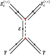
Figure 6: The corresponding Feynman diagram for the $\Xi_{c}^{(\prime,*)}\bar{T}\to\Xi_{c}^{(\prime,*)}\bar{T}$ scattering process. Here, $T$ represents either $D_{1}$ or $D_{2}^{*}$.

In our concrete calculations, we can extract the interaction vertices for the $\Xi_{c}^{(\prime,*)}\bar{T}\to\Xi_{c}^{(\prime,*)}\bar{T}$ scattering process from the constructed effective Lagrangians. The explicit expressions for the related interaction vertex functions are given below

$$\Xi_{c}\Xi_{c}\sigma : 2l_{B}m_{\Xi_{c}}\chi^{\dagger}_{3}\chi_{1},$$

$$\Xi_{c}^{\prime}\Xi_{c}^{\prime}\sigma : -2l_{S}m_{\Xi_{c}^{\prime}}\chi^{\dagger}_{3}\chi_{1},$$

$$\Xi_{c}^{*}\Xi_{c}^{*}\sigma : -2l_{S}m_{\Xi_{c}^{*}}\mathcal{A}{\bm{\epsilon}^{\dagger m_{2}^{\prime}}_{3}}\cdot{\bm{\epsilon}_{1}^{m_{2}}}\chi^{\dagger m_{1}^{\prime}}_{3}\chi_{1}^{m_{1}},$$

$$\Xi_{c}^{*}\Xi_{c}^{\prime}\sigma : \frac{2l_{S}}{\sqrt{3}}\sqrt{m_{\Xi_{c}^{*}}m_{\Xi_{c}^{\prime}}}\mathcal{B}\chi^{\dagger m_{1}}_{3}{\bm{\sigma}}\cdot{\bm{\epsilon}^{\dagger m_{2}}_{3}}\chi_{1},$$

$$\Xi_{c}^{\prime}\Xi_{c}^{\prime}\mathbb{P} : -\frac{2ig_{1}}{f_{\pi}}m_{\Xi_{c}^{\prime}}{\bm{\sigma}}\cdot{\bm{q}}\chi^{\dagger}_{3}\chi_{1},$$

$$\Xi_{c}^{*}\Xi_{c}^{*}\mathbb{P} : -\frac{3g_{1}}{f_{\pi}}m_{\Xi_{c}^{*}}\mathcal{A}\left({\bm{\epsilon}^{\dagger m_{2}^{\prime}}_{3}}\times{\bm{\epsilon}_{1}^{m_{2}}}\right)\cdot{\bm{q}}\chi^{\dagger m_{1}^{\prime}}_{3}\chi_{1}^{m_{1}},$$

$$\Xi_{c}^{\prime}\Xi_{c}\mathbb{P} : -\frac{2ig_{4}}{\sqrt{3}f_{\pi}}\sqrt{m_{\Xi_{c}^{\prime}}m_{\Xi_{c}}}\chi^{\dagger}_{3}{\bm{\sigma}}\cdot{\bm{q}}\chi_{1},$$

$$\Xi_{c}^{*}\Xi_{c}\mathbb{P} : \frac{2ig_{4}}{f_{\pi}}\sqrt{m_{\Xi_{c}^{*}}m_{\Xi_{c}}}\mathcal{B}{\bm{\epsilon}^{\dagger m_{2}}_{3}}\cdot{\bm{q}}\chi^{\dagger m_{1}}_{3}\chi_{1},$$

$$\Xi_{c}^{*}\Xi_{c}^{\prime}\mathbb{P} : \frac{\sqrt{3}g_{1}}{f_{\pi}}\sqrt{m_{\Xi_{c}^{*}}m_{\Xi_{c}^{\prime}}}\mathcal{B}\chi^{\dagger m_{1}}_{3}\left({\bm{\epsilon}^{\dagger m_{2}}_{3}}\times{\bm{\sigma}}\right)\cdot{\bm{q}}\chi_{1},$$

$$\Xi_{c}\Xi_{c}\mathbb{V} : \sqrt{2}\beta_{B}g_{V}m_{\Xi_{c}}\chi^{\dagger}_{3}\chi_{1},$$

$$\Xi_{c}^{\prime}\Xi_{c}^{\prime}\mathbb{V} : -\sqrt{2}\beta_{S}g_{V}m_{\Xi_{c}^{\prime}}\chi^{\dagger}_{3}\chi_{1}+\frac{2\sqrt{2}i\lambda_{S}g_{V}}{3}m_{\Xi_{c}^{\prime}}\chi^{\dagger}_{3}\left({\bm{\sigma}}\times{\bm{q}}\right)_{\mu}\chi_{1},$$

$$\Xi_{c}^{*}\Xi_{c}^{*}\mathbb{V} : -\sqrt{2}\beta_{S}g_{V}m_{\Xi_{c}^{*}}\mathcal{A}{\bm{\epsilon}^{\dagger m_{2}^{\prime}}_{3}}\cdot{\bm{\epsilon}_{1}^{m_{2}}}\chi^{\dagger m_{1}^{\prime}}_{3}\chi_{1}^{m_{1}}$$

$$+\sqrt{2}\lambda_{S}g_{V}m_{\Xi_{c}^{*}}\mathcal{A}$$

$$\times\left[\left({\bm{\epsilon}^{\dagger m_{2}^{\prime}}_{3}}\cdot{\bm{q}}\right)\epsilon_{1\mu}^{m_{2}}-{\epsilon^{\dagger m_{2}^{\prime}}_{3\mu}}\left(\bm{\epsilon}_{1}^{m_{2}}\cdot{\bm{q}}\right)\right]\chi^{\dagger m_{1}^{\prime}}_{3}\chi_{1}^{m_{1}},$$

$$\Xi_{c}^{\prime}\Xi_{c}\mathbb{V} : \frac{4i\lambda_{I}g_{V}}{\sqrt{6}}\sqrt{m_{\Xi_{c}^{\prime}}m_{\Xi_{c}}}\varepsilon^{0\nu\lambda\mu}\chi^{\dagger}_{3}\sigma_{\nu}q_{\lambda}\chi_{1},$$

$$\Xi_{c}^{*}\Xi_{c}\mathbb{V} : -2\sqrt{2}i\lambda_{I}g_{V}\sqrt{m_{\Xi_{c}^{*}}m_{\Xi_{c}}}\mathcal{B}\varepsilon^{0\nu\lambda\mu}\epsilon_{3\nu}^{\dagger m_{2}}q_{\lambda}\chi^{\dagger m_{1}}_{3}\chi_{1},$$

$$\Xi_{c}^{*}\Xi_{c}^{\prime}\mathbb{V} : \frac{2\beta_{S}g_{V}}{\sqrt{6}}\sqrt{m_{\Xi_{c}^{*}}m_{\Xi_{c}^{\prime}}}\mathcal{B}\chi^{\dagger m_{1}}_{3}{\bm{\epsilon}^{\dagger m_{2}}_{3}}\cdot{\bm{\sigma}}\chi_{1}$$

$$-\frac{2\lambda_{S}g_{V}}{\sqrt{6}}\sqrt{m_{\Xi_{c}^{*}}m_{\Xi_{c}^{\prime}}}\mathcal{B}\chi^{\dagger m_{1}}_{3}$$

$$\times\left[\left({\bm{\epsilon}^{\dagger m_{2}}_{3}}\cdot{\bm{q}}\right)\sigma_{1\mu}-{\epsilon^{\dagger m_{2}}_{3\mu}}\left(\bm{\sigma}\cdot{\bm{q}}\right)\right]\chi_{1},$$

$$\bar{D}_{1}\bar{D}_{1}\sigma : 2g^{\prime\prime}_{\sigma}m_{D_{1}}{\bm{\epsilon}^{\dagger}_{4}}\cdot{\bm{\epsilon}_{2}},$$

$$\bar{D}_{2}^{*}\bar{D}_{2}^{*}\sigma : 2g^{\prime\prime}_{\sigma}m_{D_{2}^{*}}\mathcal{C}\left({\bm{\epsilon}^{\dagger}_{4m}}\cdot{\bm{\epsilon}_{2a}}\right)\left({\bm{\epsilon}^{\dagger}_{4n}}\cdot{\bm{\epsilon}_{2b}}\right),$$

$$\bar{D}_{1}\bar{D}_{1}\mathbb{P} : \frac{-5k}{3f_{\pi}}m_{D_{1}}\left({\bm{\epsilon}^{\dagger}_{4}}\times{\bm{\epsilon}_{2}}\right)\cdot{\bm{q}},$$

$$\bar{D}_{2}^{*}\bar{D}_{2}^{*}\mathbb{P} : \frac{-2k}{f_{\pi}}m_{D_{2}^{*}}\mathcal{C}\left({\bm{\epsilon}^{\dagger}_{4m}}\cdot{\bm{\epsilon}_{2a}}\right)\left[\left({\bm{\epsilon}^{\dagger}_{4n}}\times{\bm{\epsilon}_{2b}}\right)\cdot{\bm{q}}\right],$$

$$\bar{D}_{2}^{*}\bar{D}_{1}\mathbb{P} : -i\sqrt{\frac{2}{3}}\frac{k}{f_{\pi}}\sqrt{m_{D_{2}^{*}}m_{D_{1}}}\mathcal{D}\left({\bm{\epsilon}^{\dagger}_{4m}}\cdot{\bm{\epsilon}_{2}}\right)\left({\bm{\epsilon}^{\dagger}_{4n}}\cdot{\bm{q}}\right),$$

$$\bar{D}_{1}\bar{D}_{1}\mathbb{V} : -\sqrt{2}\beta^{\prime\prime}g_{V}m_{D_{1}}{\bm{\epsilon}^{\dagger}_{4}}\cdot{\bm{\epsilon}_{2}}$$

$$-\frac{5\sqrt{2}\lambda^{\prime\prime}g_{V}}{3}m_{D_{1}}\left[\left({\bm{\epsilon}^{\dagger}_{4}}\cdot{\bm{q}}\right)\epsilon^{\nu}_{2}-\epsilon^{\nu\dagger}_{4}\left({\bm{\epsilon}_{2}}\cdot{\bm{q}}\right)\right],$$

$$\bar{D}_{2}^{*}\bar{D}_{2}^{*}\mathbb{V} : -\sqrt{2}\beta^{\prime\prime}g_{V}m_{D_{2}^{*}}\mathcal{C}\left({\bm{\epsilon}^{\dagger}_{4m}}\cdot{\bm{\epsilon}_{2a}}\right)\left({\bm{\epsilon}^{\dagger}_{4n}}\cdot{\bm{\epsilon}_{2b}}\right)$$

$$-2\sqrt{2}\lambda^{\prime\prime}g_{V}m_{D_{2}^{*}}\mathcal{C}\left({\bm{\epsilon}^{\dagger}_{4m}}\cdot{\bm{\epsilon}_{2a}}\right)$$

$$\times\left[\left({\bm{\epsilon}^{\dagger}_{4n}}\cdot{\bm{q}}\right)\epsilon^{\nu}_{2b}-\epsilon^{\nu\dagger}_{4n}\left({\bm{\epsilon}_{2b}}\cdot{\bm{q}}\right)\right],$$

$$\bar{D}_{2}^{*}\bar{D}_{1}\mathbb{V} : \frac{2i\lambda^{\prime\prime}g_{V}}{\sqrt{3}}\sqrt{m_{D_{2}^{*}}m_{D_{1}}}\mathcal{D}\left[3\varepsilon^{\mu 0\nu\lambda}\left({\bm{\epsilon}^{\dagger}_{4m}}\cdot{\bm{\epsilon}_{2}}\right)\epsilon_{4n\lambda}^{\dagger}q_{\mu}\right.$$

$$\left.+2\varepsilon^{\mu\lambda 0\nu}\left({\bm{\epsilon}^{\dagger}_{4m}}\cdot{\bm{q}}\right)\epsilon_{4n\mu}^{\dagger}{\epsilon_{2\lambda}}-2\left({\bm{\epsilon}^{\dagger}_{4m}}\times{\bm{\epsilon}_{2}}\right)\cdot{\bm{q}}\epsilon_{4n}^{\nu\dagger}\right].$$

In the above interaction vertex functions, we take the notations $\mathcal{A}=\sum_{m_{1},m_{2},m_{1}^{\prime},m_{2}^{\prime}}C^{\frac{3}{2},m_{1}+m_{2}}_{\frac{1}{2}m_{1},1m_{2}}C^{\frac{3}{2},m_{1}^{\prime}+m_{2}^{\prime}}_{\frac{1}{2}m_{1}^{\prime},1m_{2}^{\prime}}$, $\mathcal{B}=\sum_{m_{1},m_{2}}C^{\frac{3}{2},m_{1}+m_{2}}_{\frac{1}{2}m_{1},1m_{2}}$, $\mathcal{C}=\sum_{m,n,a,b}C^{2,m+n}_{1m,1n}C^{2,a+b}_{1a,1b}$, and $\mathcal{D}=\sum_{m,n}C^{2,m+n}_{1m,1n}$.

Appendix B The OBE effective potentials for the $\Xi_{c}^{(\prime,*)}\bar{D}_{1}/\Xi_{c}^{(\prime,*)}\bar{D}_{2}^{*}$ systems

In this appendix, we collect the obtained OBE effective potentials for the $\Xi_{c}^{(\prime,*)}\bar{D}_{1}/\Xi_{c}^{(\prime,*)}\bar{D}_{2}^{*}$ systems when considering the single channel analysis and the $S$-$D$ wave mixing analysis. Before listing the OBE effective potentials for the $\Xi_{c}^{(\prime,*)}\bar{D}_{1}/\Xi_{c}^{(\prime,*)}\bar{D}_{2}^{*}$ systems, several operators adopted in the present work are defined as

$$\mathcal{O}_{1} = {\bm{\epsilon}^{\dagger}_{4}}\cdot{\bm{\epsilon}_{2}}\chi^{\dagger}_{3}\chi_{1},$$

$$\mathcal{O}_{2} = \chi^{\dagger}_{3}\left[{\bm{\sigma}}\cdot\left(i{\bm{\epsilon}^{\dagger}_{4}}\times{\bm{\epsilon}_{2}}\right)\right]\chi_{1},$$

$$\mathcal{O}_{3} = \chi^{\dagger}_{3}T({\bm{\sigma}},i{\bm{\epsilon}^{\dagger}_{4}}\times{\bm{\epsilon}_{2}})\chi_{1},$$

$$\mathcal{O}_{4} = \mathcal{A}\left({\bm{\epsilon}^{\dagger}_{4m}}\cdot{\bm{\epsilon}_{2a}}\right)\left({\bm{\epsilon}^{\dagger}_{4n}}\cdot{\bm{\epsilon}_{2b}}\right)\chi^{\dagger}_{3}\chi_{1},$$

$$\mathcal{O}_{5} = \mathcal{A}\left({\bm{\epsilon}^{\dagger}_{4m}}\cdot{\bm{\epsilon}_{2a}}\right)\chi^{\dagger}_{3}[{\bm{\sigma}}\cdot(i{\bm{\epsilon}^{\dagger}_{4n}}\times{\bm{\epsilon}_{2b}})]\chi_{1},$$

$$\mathcal{O}_{6} = \mathcal{A}\left({\bm{\epsilon}^{\dagger}_{4m}}\cdot{\bm{\epsilon}_{2a}}\right)\chi^{\dagger}_{3}T({\bm{\sigma}},i{\bm{\epsilon}^{\dagger}_{4n}}\times{\bm{\epsilon}_{2b}})\chi_{1},$$

$$\mathcal{O}_{7} = \mathcal{B}\left({\bm{\epsilon}^{\dagger m_{2}^{\prime}}_{3}}\cdot{\bm{\epsilon}_{1}}^{m_{2}}\right)\left({\bm{\epsilon}^{\dagger}_{4}}\cdot{\bm{\epsilon}_{2}}\right)\chi^{\dagger m_{1}^{\prime}}_{3}\chi_{1}^{m_{1}},$$

$$\mathcal{O}_{8} = \mathcal{B}\left[\left({\bm{\epsilon}^{\dagger m_{2}^{\prime}}_{3}}\times{\bm{\epsilon}_{1}}^{m_{2}}\right)\cdot\left({\bm{\epsilon}^{\dagger}_{4}}\times{\bm{\epsilon}_{2}}\right)\right]\chi^{\dagger m_{1}^{\prime}}_{3}\chi_{1}^{m_{1}},$$

$$\mathcal{O}_{9} = \mathcal{B}T({\bm{\epsilon}^{\dagger m_{2}^{\prime}}_{3}}\times{\bm{\epsilon}_{1}}^{m_{2}},{\bm{\epsilon}^{\dagger}_{4}}\times{\bm{\epsilon}_{2}})\chi^{\dagger m_{1}^{\prime}}_{3}\chi_{1}^{m_{1}},$$

$$\mathcal{O}_{10} = \mathcal{A}\mathcal{B}\left({\bm{\epsilon}^{\dagger m_{2}^{\prime}}_{3}}\cdot{\bm{\epsilon}_{1}}^{m_{2}}\right)\left({\bm{\epsilon}^{\dagger}_{4m}}\cdot{\bm{\epsilon}_{2a}}\right)\left({\bm{\epsilon}^{\dagger}_{4n}}\cdot{\bm{\epsilon}_{2b}}\right)\chi^{\dagger m_{1}^{\prime}}_{3}\chi_{1}^{m_{1}},$$

$$\mathcal{O}_{11} = \mathcal{A}\mathcal{B}\left({\bm{\epsilon}^{\dagger}_{4m}}\cdot{\bm{\epsilon}_{2a}}\right)\left[\left({\bm{\epsilon}^{\dagger m_{2}^{\prime}}_{3}}\times{\bm{\epsilon}_{1}}^{m_{2}}\right)\cdot\left({\bm{\epsilon}^{\dagger}_{4n}}\times{\bm{\epsilon}_{2b}}\right)\right]\chi^{\dagger m_{1}^{\prime}}_{3}\chi_{1}^{m_{1}},$$

$$\mathcal{O}_{12} = \mathcal{A}\mathcal{B}\left({\bm{\epsilon}^{\dagger}_{4m}}\cdot{\bm{\epsilon}_{2a}}\right)T({\bm{\epsilon}^{\dagger m_{2}^{\prime}}_{3}}\times{\bm{\epsilon}_{1}}^{m_{2}},{\bm{\epsilon}^{\dagger}_{4n}}\times{\bm{\epsilon}_{2b}})\chi^{\dagger m_{1}^{\prime}}_{3}\chi_{1}^{m_{1}}.$$

In the above defined operators, we use the notations $\mathcal{A}=\sum_{m,n,a,b}C^{2,m+n}_{1m,1n}C^{2,a+b}_{1a,1b}$ and $\mathcal{B}=\sum_{m_{1},m_{2},m_{1}^{\prime},m_{2}^{\prime}}C^{\frac{3}{2},m_{1}+m_{2}}_{\frac{1}{2}m_{1},1m_{2}}C^{\frac{3}{2},m_{1}^{\prime}+m_{2}^{\prime}}_{\frac{1}{2}m_{1}^{\prime},1m_{2}^{\prime}}$. In addition, the tensor force operator $T({\bm{x}},{\bm{y}})$ is $T({\bm{x}},{\bm{y}})=3\left(\hat{\bm{r}}\cdot{\bm{x}}\right)\left(\hat{\bm{r}}\cdot{\bm{y}}\right)-{\bm{x}}\cdot{\bm{y}}$. In the concrete calculations, these defined operators $\mathcal{O}_{i}$ should be sandwiched by the corresponding spin-orbital wave functions $|{}^{2S+1}L_{J}\rangle$ of the initial and final states listed in Eq. (LABEL:spinorbitalwavefunctions), where the obtained operator matrix elements are summarized in Table 10.

Table 10: The obtained operator matrix elements in the OBE effective potentials when considering the $S$-$D$ wave mixing effect.

$J^{P}$	$1/2^{+}$	$3/2^{+}$	$5/2^{+}$	$7/2^{+}$
$\mathcal{O}_{1}$	Diag(1,1)	Diag(1,1,1)
$\mathcal{O}_{2}$	Diag(2,$-1$)	Diag($-1$,2,$-1$)
$\mathcal{O}_{3}$	$\left(\begin{array}[]{cc}0&\sqrt{2}\\ \sqrt{2}&2\end{array}\right)$	$\left(\begin{array}[]{ccc}0&-1&-2\\ -1&0&1\\ -2&1&0\end{array}\right)$
$\mathcal{O}_{4}$		Diag(1,1,1)	Diag(1,1,1)
$\mathcal{O}_{5}$		Diag($\frac{3}{2}$,$\frac{3}{2}$,$-1$)	Diag($-1$,$\frac{3}{2}$,$-1$)
$\mathcal{O}_{6}$		$\left(\begin{array}[]{ccc}0&\frac{3}{5}&\frac{3\sqrt{21}}{10}\\ \frac{3}{5}&0&\frac{3\sqrt{21}}{14}\\ \frac{3\sqrt{21}}{10}&\frac{3\sqrt{21}}{14}&\frac{4}{7}\end{array}\right)$	$\left(\begin{array}[]{ccc}0&-\frac{3\sqrt{14}}{10}&-\frac{2\sqrt{14}}{5}\\ -\frac{3\sqrt{14}}{10}&\frac{3}{7}&\frac{3}{7}\\ -\frac{2\sqrt{14}}{5}&\frac{3}{7}&-\frac{4}{7}\end{array}\right)$
$\mathcal{O}_{7}$	Diag(1,1,1)	Diag(1,1,1,1)	Diag(1,1,1,1)
$\mathcal{O}_{8}$	Diag($\frac{5}{3}$,$\frac{2}{3}$,$-1$)	Diag($\frac{2}{3}$,$\frac{5}{3}$,$\frac{2}{3}$,$-1$)	Diag($-1$,$\frac{5}{3}$,$\frac{2}{3}$,$-1$)
$\mathcal{O}_{9}$	$\left(\begin{array}[]{ccc}0&-\frac{7}{3\sqrt{5}}&\frac{2}{\sqrt{5}}\\ -\frac{7}{3\sqrt{5}}&\frac{16}{15}&-\frac{1}{5}\\ \frac{2}{\sqrt{5}}&-\frac{1}{5}&\frac{8}{5}\end{array}\right)$	$\left(\begin{array}[]{cccc}0&\frac{7}{3\sqrt{10}}&-\frac{16}{15}&-\frac{\sqrt{7}}{5\sqrt{2}}\\ \frac{7}{3\sqrt{10}}&0&-\frac{7}{3\sqrt{10}}&-\frac{2}{\sqrt{35}}\\ -\frac{16}{15}&-\frac{7}{3\sqrt{10}}&0&-\frac{1}{\sqrt{14}}\\ -\frac{\sqrt{7}}{5\sqrt{2}}&-\frac{2}{\sqrt{35}}&-\frac{1}{\sqrt{14}}&\frac{4}{7}\end{array}\right)$	$\left(\begin{array}[]{cccc}0&\frac{2}{\sqrt{15}}&\frac{\sqrt{7}}{5\sqrt{3}}&-\frac{2\sqrt{14}}{5}\\ \frac{2}{\sqrt{15}}&0&\frac{\sqrt{7}}{3\sqrt{5}}&-\frac{4\sqrt{2}}{\sqrt{105}}\\ \frac{\sqrt{7}}{5\sqrt{3}}&\frac{\sqrt{7}}{3\sqrt{5}}&-\frac{16}{21}&-\frac{\sqrt{2}}{7\sqrt{3}}\\ -\frac{2\sqrt{14}}{5}&-\frac{4\sqrt{2}}{\sqrt{105}}&-\frac{\sqrt{2}}{7\sqrt{3}}&-\frac{4}{7}\end{array}\right)$
$\mathcal{O}_{10}$	Diag(1,1,1)	Diag(1,1,1,1,1)	Diag(1,1,1,1,1)	Diag(1,1,1,1)
$\mathcal{O}_{11}$	Diag($\frac{3}{2}$,1,$\frac{1}{6}$)	Diag(1,$\frac{3}{2}$,1,$\frac{1}{6}$,$-1$)	Diag($\frac{1}{6}$,$\frac{3}{2}$,1,$\frac{1}{6}$,$-1$)	Diag($-1$,1,$\frac{1}{6}$,$-1$)
$\mathcal{O}_{12}$	$\left(\begin{array}[]{ccc}0&\frac{9}{10}&\frac{\sqrt{21}}{5}\\ \frac{9}{10}&\frac{4}{5}&\frac{3\sqrt{21}}{70}\\ \frac{\sqrt{21}}{5}&\frac{3\sqrt{21}}{70}&\frac{116}{105}\end{array}\right)$	$\left(\begin{array}[]{ccccc}0&-\frac{9\sqrt{2}}{20}&-\frac{4}{5}&\frac{3\sqrt{6}}{20}&\frac{2\sqrt{2}}{5}\\ -\frac{9\sqrt{2}}{20}&0&\frac{9\sqrt{2}}{20}&-\frac{\sqrt{3}}{5}&0\\ -\frac{4}{5}&\frac{9\sqrt{2}}{20}&0&\frac{3\sqrt{6}}{28}&-\frac{4\sqrt{2}}{35}\\ \frac{3\sqrt{6}}{20}&-\frac{\sqrt{3}}{5}&\frac{3\sqrt{6}}{28}&\frac{58}{147}&\frac{18\sqrt{3}}{245}\\ \frac{2\sqrt{2}}{5}&0&-\frac{4\sqrt{2}}{35}&\frac{18\sqrt{3}}{245}&\frac{60}{49}\end{array}\right)$	$\left(\begin{array}[]{ccccc}0&\frac{\sqrt{7}}{5}&-\frac{3}{10}&-\frac{29\sqrt{2}}{15\sqrt{7}}&\frac{\sqrt{6}}{5\sqrt{7}}\\ \frac{\sqrt{7}}{5}&0&\frac{-9}{10\sqrt{7}}&-\frac{2\sqrt{2}}{5}&0\\ -\frac{3}{10}&-\frac{9}{10\sqrt{7}}&-\frac{4}{7}&\frac{3}{7\sqrt{14}}&-\frac{12\sqrt{6}}{35\sqrt{7}}\\ -\frac{29\sqrt{2}}{15\sqrt{7}}&-\frac{2\sqrt{2}}{5}&\frac{3}{7\sqrt{14}}&-\frac{58}{147}&\frac{17\sqrt{3}}{245}\\ \frac{\sqrt{6}}{5\sqrt{7}}&0&-\frac{12\sqrt{6}}{35\sqrt{7}}&\frac{17\sqrt{3}}{245}&\frac{10}{49}\end{array}\right)$	$\left(\begin{array}[]{cccc}0&\frac{2}{5}&-\frac{3}{5\sqrt{14}}&-\frac{2\sqrt{21}}{7}\\ \frac{2}{5}&\frac{8}{35}&-\frac{\sqrt{27}}{35\sqrt{14}}&-\frac{4\sqrt{21}}{49}\\ -\frac{3}{5\sqrt{14}}&-\frac{27}{35\sqrt{14}}&-\frac{493}{735}&\frac{\sqrt{3}}{49\sqrt{2}}\\ -\frac{2\sqrt{21}}{7}&-\frac{4\sqrt{21}}{49}&\frac{\sqrt{3}}{49\sqrt{2}}&-\frac{32}{49}\end{array}\right)$

For simplicity, we define the following relations in the obtained OBE effective potentials

$$\mathcal{H}(I)Y_{\mathbb{P}} = \mathcal{H}_{1}(I)Y_{\pi}+\mathcal{H}_{2}(I)Y_{\eta},$$ (2.1)

$$\mathcal{G}(I)Y_{\mathbb{V}} = \mathcal{G}_{1}(I)Y_{\rho}+\mathcal{G}_{2}(I)Y_{\omega}.$$ (2.2)

Here, the isospin factors $\mathcal{H}(I)$ and $\mathcal{G}(I)$ are introduced for the $\Xi_{c}^{(\prime,*)}\bar{D}_{1}/\Xi_{c}^{(\prime,*)}\bar{D}_{2}^{*}$ systems, and $I$ stands for the corresponding isospin quantum number. For the $\Xi_{c}\bar{D}_{1}/\Xi_{c}\bar{D}_{2}^{*}$ systems, we can obtain

$$\mathcal{G}_{1}(I=0) = -3/2,~{}~{}~{}~{}\mathcal{G}_{1}(I=1)=1/2,$$

$$\mathcal{G}_{2}(I=0) = 1/2,~{}~{}~{}~{}~{}~{}~{}\mathcal{G}_{2}(I=1)=1/2.$$ (2.3)

For the $\Xi_{c}^{\prime(*)}\bar{D}_{1}/\Xi_{c}^{\prime(*)}\bar{D}_{2}^{*}$ systems, we can get

$$\mathcal{H}_{1}(I=0) = -3/4,~{}~{}~{}~{}~{}~{}\mathcal{H}_{1}(I=1)=1/4,$$

$$\mathcal{H}_{2}(I=0) = -1/12,~{}~{}~{}~{}\mathcal{H}_{2}(I=1)=-1/12,$$

$$\mathcal{G}_{1}(I=0) = -3/4,~{}~{}~{}~{}~{}~{}~{}\mathcal{G}_{1}(I=1)=1/4,$$

$$\mathcal{G}_{2}(I=0) = 1/4,~{}~{}~{}~{}~{}~{}~{}~{}~{}~{}\mathcal{G}_{2}(I=1)=1/4.$$ (2.4)

In the above defined relations, the Yukawa potential considering the monopole-type form factor $Y_{\mathcal{E}}$ can be written as

$$Y_{\mathcal{E}}=\frac{e^{-m_{\mathcal{E}}r}-e^{-\Lambda r}}{4\pi r}-\frac{\Lambda^{2}-m_{\mathcal{E}}^{2}}{8\pi\Lambda}e^{-\Lambda r},$$ (2.5)

where $\Lambda$ is the cutoff parameter in the monopole-type form factor, and $m_{\mathcal{E}}$ is the mass of the exchanged light meson $\mathcal{E}$.

The OBE effective potentials in the coordinate space for the $\Xi_{c}^{(\prime,*)}\bar{D}_{1}/\Xi_{c}^{(\prime,*)}\bar{D}_{2}^{*}$ systems are given by

$$\mathcal{V}^{\Xi_{c}\bar{D}_{1}\rightarrow\Xi_{c}\bar{D}_{1}} = -2l_{B}g_{\sigma}^{\prime\prime}\mathcal{O}_{1}Y_{\sigma}-\frac{1}{2}\beta_{B}\beta^{\prime\prime}g_{V}^{2}\mathcal{O}_{1}\mathcal{G}(I)Y_{\mathbb{V}},$$ (2.6)

$$\mathcal{V}^{\Xi_{c}\bar{D}_{2}^{*}\rightarrow\Xi_{c}\bar{D}_{2}^{*}} = -2l_{B}g_{\sigma}^{\prime\prime}\mathcal{O}_{4}Y_{\sigma}-\frac{1}{2}\beta_{B}\beta^{\prime\prime}g_{V}^{2}\mathcal{O}_{4}\mathcal{G}(I)Y_{\mathbb{V}},$$ (2.7)

$$\mathcal{V}^{\Xi_{c}^{\prime}\bar{D}_{1}\rightarrow\Xi_{c}^{\prime}\bar{D}_{1}} = l_{S}g_{\sigma}^{\prime\prime}\mathcal{O}_{1}Y_{\sigma}+\frac{1}{2}\beta_{S}\beta^{\prime\prime}g_{V}^{2}\mathcal{O}_{1}\mathcal{G}(I)Y_{\mathbb{V}}$$

$$+\frac{5}{18}\frac{g_{1}k}{f_{\pi}^{2}}\left[\mathcal{O}_{2}\nabla^{2}+\mathcal{O}_{3}r\frac{\partial}{\partial r}\frac{1}{r}\frac{\partial}{\partial r}\right]\mathcal{H}(I)Y_{\mathbb{P}}$$

$$-\frac{5}{27}\lambda_{S}\lambda^{\prime\prime}g_{V}^{2}\left[2\mathcal{O}_{2}\nabla^{2}-\mathcal{O}_{3}r\frac{\partial}{\partial r}\frac{1}{r}\frac{\partial}{\partial r}\right]\mathcal{G}(I)Y_{\mathbb{V}},$$

$$\mathcal{V}^{\Xi_{c}^{\prime}\bar{D}_{2}^{*}\rightarrow\Xi_{c}^{\prime}\bar{D}_{2}^{*}} = l_{S}g_{\sigma}^{\prime\prime}\mathcal{O}_{4}Y_{\sigma}+\frac{1}{2}\beta_{S}\beta^{\prime\prime}g_{V}^{2}\mathcal{O}_{4}\mathcal{G}(I)Y_{\mathbb{V}}$$

$$+\frac{1}{3}\frac{g_{1}k}{f_{\pi}^{2}}\left[\mathcal{O}_{5}\nabla^{2}+\mathcal{O}_{6}r\frac{\partial}{\partial r}\frac{1}{r}\frac{\partial}{\partial r}\right]\mathcal{H}(I)Y_{\mathbb{P}}$$

$$-\frac{2}{9}\lambda_{S}\lambda^{\prime\prime}g_{V}^{2}\left[2\mathcal{O}_{5}\nabla^{2}-\mathcal{O}_{6}r\frac{\partial}{\partial r}\frac{1}{r}\frac{\partial}{\partial r}\right]\mathcal{G}(I)Y_{\mathbb{V}},$$

$$\mathcal{V}^{\Xi_{c}^{*}\bar{D}_{1}\rightarrow\Xi_{c}^{*}\bar{D}_{1}} = l_{S}g_{\sigma}^{\prime\prime}\mathcal{O}_{7}Y_{\sigma}+\frac{1}{2}\beta_{S}\beta^{\prime\prime}g_{V}^{2}\mathcal{O}_{7}\mathcal{G}(I)Y_{\mathbb{V}}$$

$$+\frac{5}{12}\frac{g_{1}k}{f_{\pi}^{2}}\left[\mathcal{O}_{8}\nabla^{2}+\mathcal{O}_{9}r\frac{\partial}{\partial r}\frac{1}{r}\frac{\partial}{\partial r}\right]\mathcal{H}(I)Y_{\mathbb{P}}$$

$$-\frac{5}{18}\lambda_{S}\lambda^{\prime\prime}g_{V}^{2}\left[2\mathcal{O}_{8}\nabla^{2}-\mathcal{O}_{9}r\frac{\partial}{\partial r}\frac{1}{r}\frac{\partial}{\partial r}\right]\mathcal{G}(I)Y_{\mathbb{V}},$$

$$\mathcal{V}^{\Xi_{c}^{*}\bar{D}_{2}^{*}\rightarrow\Xi_{c}^{*}\bar{D}_{2}^{*}} = l_{S}g_{\sigma}^{\prime\prime}\mathcal{O}_{10}Y_{\sigma}+\frac{1}{2}\beta_{S}\beta^{\prime\prime}g_{V}^{2}\mathcal{O}_{10}\mathcal{G}(I)Y_{\mathbb{V}}$$

$$+\frac{1}{2}\frac{g_{1}k}{f_{\pi}^{2}}\left[\mathcal{O}_{11}\nabla^{2}+\mathcal{O}_{12}r\frac{\partial}{\partial r}\frac{1}{r}\frac{\partial}{\partial r}\right]\mathcal{H}(I)Y_{\mathbb{P}}$$

$$-\frac{1}{3}\lambda_{S}\lambda^{\prime\prime}g_{V}^{2}\left[2\mathcal{O}_{11}\nabla^{2}-\mathcal{O}_{12}r\frac{\partial}{\partial r}\frac{1}{r}\frac{\partial}{\partial r}\right]\mathcal{G}(I)Y_{\mathbb{V}}.$$

In the above OBE effective potentials, the superscript is used to mark the corresponding scattering process.

References

- (1) M. Gell-Mann, A Schematic Model of Baryons and Mesons, Phys. Lett. 8, 214 (1964).
- (2) G. Zweig, An SU(3) model for strong interaction symmetry and its breaking. Version 1, CERN-TH-401.
- (3) X. Liu, An overview of new particles, Chin. Sci. Bull. 59, 3815 (2014).
- (4) A. Hosaka, T. Iijima, K. Miyabayashi, Y. Sakai, and S. Yasui, Exotic hadrons with heavy flavors: , , , and related states, Prog. Theor. Exp. Phys. 2016, 062C01 (2016).
- (5) H. X. Chen, W. Chen, X. Liu, and S. L. Zhu, The hidden-charm pentaquark and tetraquark states, Phys. Rep. 639, 1 (2016).
- (6) J. M. Richard, Exotic hadrons: review and perspectives, Few Body Syst. 57, 1185-1212 (2016).
- (7) R. F. Lebed, R. E. Mitchell and E. S. Swanson, Heavy-Quark QCD Exotica, Prog. Part. Nucl. Phys. 93, 143-194 (2017).
- (8) S. L. Olsen, T. Skwarnicki, and D. Zieminska, Nonstandard heavy mesons and baryons: Experimental evidence, Rev. Mod. Phys. 90, 015003 (2018).
- (9) F. K. Guo, C. Hanhart, U. G. Meiner, Q. Wang, Q. Zhao, and B. S. Zou, Hadronic molecules, Rev. Mod. Phys. 90, 015004 (2018).
- (10) Y. R. Liu, H. X. Chen, W. Chen, X. Liu, and S. L. Zhu, Pentaquark and tetraquark states, Prog. Part. Nucl. Phys. 107, 237 (2019).
- (11) N. Brambilla, S. Eidelman, C. Hanhart, A. Nefediev, C. P. Shen, C. E. Thomas, A. Vairo, and C. Z. Yuan, The states: Experimental and theoretical status and perspectives, Phys. Rep. 873, 1 (2020).
- (12) L. Meng, B. Wang, G. J. Wang and S. L. Zhu, Chiral perturbation theory for heavy hadrons and chiral effective field theory for heavy hadronic molecules, Phys. Rept. 1019, 1-149 (2023).
- (13) H. X. Chen, W. Chen, X. Liu, Y. R. Liu and S. L. Zhu, An updated review of the new hadron states, Rept. Prog. Phys. 86, no.2, 026201 (2023).
- (14) T. Gershon [LHCb], Exotic hadron naming convention, arXiv:2206.15233.
- (15) R. Aaij et al. (LHCb Collaboration), Observation of resonances consistent with pentaquark states in decays, Phys. Rev. Lett. 115, 072001 (2015).
- (16) R. Aaij et al. (LHCb Collaboration), Observation of a narrow pentaquark state, , and of two-peak structure of the , Phys. Rev. Lett. 122, 222001 (2019).
- (17) R. Aaij et al.(LHCb Collaboration), Evidence of a structure and observation of excited states in the decay, Sci. Bull. 66, 1278-1287 (2021).
- (18) [LHCb], Observation of a resonance consistent with a strange pentaquark candidate in decays, arXiv:2210.10346
- (19) J. J. Wu, R. Molina, E. Oset and B. S. Zou, Prediction of narrow and resonances with hidden charm above 4 GeV, Phys. Rev. Lett. 105, 232001 (2010).
- (20) W. L. Wang, F. Huang, Z. Y. Zhang, and B. S. Zou, and states in a chiral quark model, Phys. Rev. C 84, 015203 (2011).
- (21) Z. C. Yang, Z. F. Sun, J. He, X. Liu, and S. L. Zhu, The possible hidden-charm molecular baryons composed of anticharmed meson and charmed baryon, Chin. Phys. C 36, 6 (2012).
- (22) J. J. Wu, T.-S. H. Lee, and B. S. Zou, Nucleon resonances with hidden charm in coupled-channel Models, Phys. Rev. C 85, 044002 (2012).
- (23) X. Q. Li and X. Liu, A possible global group structure for exotic states, Eur. Phys. J. C 74, 3198 (2014).
- (24) R. Chen, X. Liu, X. Q. Li, and S. L. Zhu, Identifying Exotic Hidden-Charm Pentaquarks, Phys. Rev. Lett. 115, 132002 (2015).
- (25) M. Karliner and J. L. Rosner, New Exotic Meson and Baryon Resonances from Doubly-Heavy Hadronic Molecules, Phys. Rev. Lett. 115, 122001 (2015).
- (26) J. Hofmann and M. F. M. Lutz, Coupled-channel study of crypto-exotic baryons with charm, Nucl. Phys. A 763, 90 (2005).
- (27) Q. Zhang, B. R. He, and J. L. Ping, Pentaquarks with the configuration in the Chiral Quark Model, arXiv:2006.01042.
- (28) J. J. Wu, R. Molina, E. Oset and B. S. Zou, Dynamically generated and resonances in the hidden charm sector around 4.3 GeV, Phys. Rev. C 84, 015202 (2011).
- (29) V. V. Anisovich, M. A. Matveev, J. Nyiri, A. V. Sarantsev, and A. N. Semenova, Nonstrange and strange pentaquarks with hidden charm, Int. J. Mod. Phys. A 30, 1550190 (2015).
- (30) Z. G. Wang, Analysis of the pentaquark states in the diquark-diquark-antiquark model with QCD sum rules, Eur. Phys. J. C 76, 142 (2016).
- (31) A. Feijoo, V. K. Magas, A. Ramos, and E. Oset, A hidden-charm pentaquark from the decay of into states, Eur. Phys. J. C 76, no. 8, 446 (2016).
- (32) J. X. Lu, E. Wang, J. J. Xie, L. S. Geng, and E. Oset, The reaction and a hidden-charm pentaquark state with strangeness, Phys. Rev. D 93, 094009 (2016).
- (33) H. X. Chen, L. S. Geng, W. H. Liang, E. Oset, E. Wang, and J. J. Xie, Looking for a hidden-charm pentaquark state with strangeness from decay into , Phys. Rev. C 93, 065203 (2016).
- (34) R. Chen, J. He, and X. Liu, Possible strange hidden-charm pentaquarks from and interactions, Chin. Phys. C 41, 103105 (2017).
- (35) X. Z. Weng, X. L. Chen, W. Z. Deng and S. L. Zhu, Hidden-charm pentaquarks and states, Phys. Rev. D 100, no.1, 016014 (2019).
- (36) C. W. Xiao, J. Nieves, and E. Oset, Prediction of hidden charm strange molecular baryon states with heavy quark spin symmetry, Phys. Lett. B 799, 135051 (2019).
- (37) C. W. Shen, H. J. Jing, F. K. Guo, and J. J. Wu, Exploring possible triangle singularities in the decay, Symmetry 12, 1611 (2020).
- (38) B. Wang, L. Meng, and S. L. Zhu, Spectrum of the strange hidden charm molecular pentaquarks in chiral effective field theory, Phys. Rev. D 101, 034018 (2020).
- (39) H. X. Chen, W. Chen, X. Liu and X. H. Liu, Establishing the first hidden-charm pentaquark with strangeness, Eur. Phys. J. C 81, no.5, 409 (2021).
- (40) F. Z. Peng, M. J. Yan, M. Sánchez Sánchez and M. P. Valderrama, The pentaquark from a combined effective field theory and phenomenological perspective, Eur. Phys. J. C 81, no.7, 666 (2021).
- (41) R. Chen, Can the newly reported be a strange hidden-charm molecular pentaquark?, Phys. Rev. D 103, no.5, 054007 (2021).
- (42) M. Z. Liu, Y. W. Pan, and L. S. Geng, Can discovery of hidden charm strange pentaquark states help determine the spins of and ?, Phys. Rev. D 103, 034003 (2021).
- (43) C. W. Xiao, J. J. Wu and B. S. Zou, Molecular nature of and its heavy quark spin partners, Phys. Rev. D 103, no.5, 054016 (2021).
- (44) M. L. Du, Z. H. Guo and J. A. Oller, Insights into the nature of the , Phys. Rev. D 104, no.11, 114034 (2021).
- (45) J. T. Zhu, L. Q. Song and J. He, and other possible molecular states from and interactions, Phys. Rev. D 103, no.7, 074007 (2021).
- (46) X. K. Dong, F. K. Guo and B. S. Zou, A survey of heavy-antiheavy hadronic molecules, Progr. Phys. 41, 65-93 (2021).
- (47) J. F. Giron and R. F. Lebed, Fine structure of pentaquark multiplets in the dynamical diquark model, Phys. Rev. D 104, no.11, 114028 (2021).
- (48) C. Cheng, F. Yang and Y. Huang, Searching for strange hidden-charm pentaquark state in reaction, Phys. Rev. D 104, no.11, 116007 (2021).
- (49) F. Yang, Y. Huang and H. Q. Zhu, Strong decays of the as a molecule, Sci. China Phys. Mech. Astron. 64, no.12, 121011 (2021).
- (50) M. W. Li, Z. W. Liu, Z. F. Sun and R. Chen, Magnetic moments and transition magnetic moments of and states, Phys. Rev. D 104, no.5, 054016 (2021).
- (51) J. X. Lu, M. Z. Liu, R. X. Shi and L. S. Geng, Understanding as a hadronic molecule in the decay, Phys. Rev. D 104, no.3, 034022 (2021).
- (52) B. S. Zou, Building up the spectrum of pentaquark states as hadronic molecules, Sci. Bull. 66, 1258 (2021).
- (53) Z. G. Wang and Q. Xin, Analysis of hidden-charm pentaquark molecular states with and without strangeness via the QCD sum rules, Chin. Phys. C 45, no.12, 123105 (2021).
- (54) Q. Wu, D. Y. Chen and R. Ji, Production of from Decay, Chin. Phys. Lett. 38, no.7, 071301 (2021).
- (55) S. Clymton, H. J. Kim and H. C. Kim, Production of hidden-charm strange pentaquarks from the reaction, Phys. Rev. D 104, no.1, 014023 (2021).
- (56) U. Özdem, Magnetic dipole moments of the hidden-charm pentaquark states: , and , Eur. Phys. J. C 81, no.4, 277 (2021).
- (57) R. Chen, Strong decays of the newly as a strange hidden-charm molecule, Eur. Phys. J. C 81, no.2, 122 (2021).
- (58) K. Azizi, Y. Sarac and H. Sundu, Investigation of pentaquark via its strong decay to , Phys. Rev. D 103, no.9, 094033 (2021).
- (59) Z. G. Wang, Analysis of the as the hidden-charm pentaquark state with QCD sum rules, Int. J. Mod. Phys. A 36, no.10, 2150071 (2021).
- (60) K. Chen, R. Chen, L. Meng, B. Wang and S. L. Zhu, Systematics of the heavy flavor hadronic molecules, Eur. Phys. J. C 82, no.7, 581 (2022).
- (61) H. X. Chen, Hidden-charm pentaquark states through current algebra: from their production to decay, Chin. Phys. C 46, no.9, 093105 (2022).
- (62) R. Chen and X. Liu, Mass behavior of hidden-charm open-strange pentaquarks inspired by the established molecular states, Phys. Rev. D 105, no.1, 014029 (2022).
- (63) K. Chen, B. Wang and S. L. Zhu, Heavy flavor molecular states with strangeness, Phys. Rev. D 105, no.9, 096004 (2022).
- (64) X. Hu and J. Ping, Investigation of hidden-charm pentaquarks with strangeness , Eur. Phys. J. C 82, no.2, 118 (2022).
- (65) H. Garcilazo and A. Valcarce, Hidden-flavor pentaquarks, Phys. Rev. D 106, no.11, 114012 (2022).
- (66) Z. Y. Yang, F. Z. Peng, M. J. Yan, M. Sánchez Sánchez and M. Pavon Valderrama, Molecular pentaquarks from light-meson exchange saturation, arXiv:2211.08211.
- (67) K. Chen, Z. Y. Lin and S. L. Zhu, Comparison between the and systems, Phys. Rev. D 106, no.11, 116017 (2022).
- (68) A. Giachino, A. Hosaka, E. Santopinto, S. Takeuchi, M. Takizawa and Y. Yamaguchi, Rich structure of the hidden-charm pentaquarks near threshold regions, arXiv:2209.10413.
- (69) S. X. Nakamura and J. J. Wu, Pole determination of and possible in , arXiv:2208.11995.
- (70) M. Karliner and J. R. Rosner, strange pentaquarks, Phys. Rev. D 106, 036024 (2022).
- (71) F. L. Wang and X. Liu, Emergence of molecular-type characteristic spectrum of hidden-charm pentaquark with strangeness embodied in the and , Phys. Lett. B 835, 137583 (2022).
- (72) F. L. Wang, H. Y. Zhou, Z. W. Liu and X. Liu, What can we learn from the electromagnetic properties of hidden-charm molecular pentaquarks with single strangeness?, Phys. Rev. D 106, no.5, 054020 (2022).
- (73) F. Z. Peng, M. Z. Liu, Y. W. Pan, M. Sánchez Sánchez and M. Pavon Valderrama, Five-flavor pentaquarks and other light- and heavy-flavor symmetry partners of the LHCb hidden-charm pentaquarks, Nucl. Phys. B 983, 115936 (2022).
- (74) C. W. Xiao, J. Nieves, E. Oset, J. J. Wu and B. S. Zou, Is one state or two?, Rev. Mex. Fis. Suppl. 3, no.3, 0308045 (2022).
- (75) X. W. Wang and Z. G. Wang, Study of isospin eigenstates of the pentaquark molecular states with strangeness, Int. J. Mod. Phys. A 37, no.31n32, 2250189 (2022).
- (76) S. Clymton, H. J. Kim and H. C. Kim, The effect of hidden-charm strange pentaquarks on the reaction, Rev. Mex. Fis. Suppl. 3, no.3, 0308040 (2022).
- (77) F. Gao and H. S. Li, Magnetic moments of hidden-charm strange pentaquark states, Chin. Phys. C 46, no.12, 123111 (2022).
- (78) J. Ferretti and E. Santopinto, The new , , and and the possible emergence of flavor pentaquark octets and tetraquark nonets, Sci. Bull. 67, 1209 (2022).
- (79) E. Y. Paryev, On the possibility of testing the two-peak structure of the LHCb hidden-charm strange pentaquark in near-threshold antikaon-induced charmonium production on protons and nuclei, Nucl. Phys. A 1037, 122687 (2023).
- (80) K. Azizi, Y. Sarac and H. Sundu, Investigation of the strange pentaquark candidate recently observed by LHCb, arXiv:2304.00604.
- (81) U. Ozdem, Electromagnetic properties of , , and pentaquarks, arXiv:2303.10649.
- (82) A. Feijoo, W. F. Wang, C. W. Xiao, J. J. Wu, E. Oset, J. Nieves and B. S. Zou, A new look at the states from a molecular perspective, Phys. Lett. B 839, 137760 (2023).
- (83) J. T. Zhu, S. Y. Kong and J. He, and as molecular states in invariant mass spectra, Phys. Rev. D 107, no.3, 034029 (2023).
- (84) P. G. Ortega, D. R. Entem and F. Fernandez, Strange hidden-charm and pentaquarks and additional , and candidates in a quark model approach, Phys. Lett. B 838, 137747 (2023).
- (85) U. Özdem, Investigation of magnetic moment of and pentaquark states, Phys. Lett. B 836, 137635 (2023).
- (86) L. Meng, B. Wang and S. L. Zhu, Double thresholds distort the line shapes of the resonance, Phys. Rev. D 107, no.1, 014005 (2023).
- (87) M. J. Yan, F. Z. Peng, M. Sánchez Sánchez and M. Pavon Valderrama, pentaquark and its partners in the molecular picture, Phys. Rev. D 107, no.7, 074025 (2023).
- (88) X. W. Wang and Z. G. Wang, Analysis of and related pentaquark molecular states via QCD sum rules, Chin. Phys. C 47, no.1, 013109 (2023).
- (89) T. J. Burns and E. S. Swanson, The LHCb state as a triangle singularity, Phys. Lett. B 838, 137715 (2023).
- (90) R. L. Workman et al. [Particle Data Group], Review of Particle Physics, PTEP 2022, 083C01 (2022).
- (91) M. B. Wise, Chiral perturbation theory for hadrons containing a heavy quark, Phys. Rev. D 45, R2188 (1992).
- (92) R. Casalbuoni, A. Deandrea, N. Di Bartolomeo, R. Gatto, F. Feruglio, and G. Nardulli, Light vector resonances in the effective chiral Lagrangian for heavy mesons, Phys. Lett. B 292, 371 (1992).
- (93) T. M. Yan, H. Y. Cheng, C. Y. Cheung, G. L. Lin, Y. C. Lin, and H. L. Yu, Heavy quark symmetry and chiral dynamics, Phys. Rev. D 46, 1148 (1992); [Phys. Rev. D 55, 5851E (1997)].
- (94) R. Casalbuoni, A. Deandrea, N. Di Bartolomeo, R. Gatto, F. Feruglio, and G. Nardulli, Phenomenology of heavy meson chiral Lagrangians, Phys. Rep. 281, 145 (1997).
- (95) M. Bando, T. Kugo and K. Yamawaki, Nonlinear Realization and Hidden Local Symmetries, Phys. Rept. 164, 217 (1988).
- (96) M. Harada and K. Yamawaki, Hidden local symmetry at loop: A New perspective of composite gauge boson and chiral phase transition, Phys. Rept. 381, 1 (2003).
- (97) R. Chen, A. Hosaka, and X. Liu, Searching for possible -like molecular states from meson-baryon interaction, Phys. Rev. D 97, 036016 (2018).
- (98) G. J. Ding, Are and (4250) or hadronic molecules? Phys. Rev. D 79, 014001 (2009).
- (99) D. O. Riska and G. E. Brown, Nucleon resonance transition couplings to vector mesons, Nucl. Phys. A 679, 577 (2001).
- (100) R. Chen, F. L. Wang, A. Hosaka and X. Liu, Exotic triple-charm deuteronlike hexaquarks, Phys. Rev. D 97, 114011 (2018).
- (101) F. L. Wang, R. Chen, Z. W. Liu, and X. Liu, Possible triple-charm molecular pentaquarks from interactions, Phys. Rev. D 99, 054021 (2019).
- (102) R. Chen, Z. F. Sun, X. Liu and S. L. Zhu, Strong LHCb evidence supporting the existence of the hidden-charm molecular pentaquarks, Phys. Rev. D 100, no. 1, 011502 (2019).
- (103) F. L. Wang and X. Liu, Exotic double-charm molecular states with hidden or open strangeness and around GeV, Phys. Rev. D 102, 094006 (2020).
- (104) F. L. Wang, R. Chen, Z. W. Liu, and X. Liu, Probing new types of states inspired by the interaction between wave charmed baryon and anticharmed meson in a doublet, Phys. Rev. C 101, 025201 (2020).
- (105) F. L. Wang and X. Liu, Investigating new type of doubly charmed molecular tetraquarks composed of charmed mesons in the and doublets, Phys. Rev. D 104, no.9, 094030 (2021).
- (106) F. L. Wang, X. D. Yang, R. Chen and X. Liu, Correlation of the hidden-charm molecular tetraquarks and the charmoniumlike structures existing in the process, Phys. Rev. D 104, no.9, 094010 (2021).
- (107) F. L. Wang, R. Chen, and X. Liu, Prediction of hidden-charm pentaquarks with double strangeness, Phys. Rev. D 103, 034014 (2021).
- (108) F. L. Wang, X. D. Yang, R. Chen and X. Liu, Hidden-charm pentaquarks with triple strangeness due to the interactions, Phys. Rev. D 103, 054025 (2021).
- (109) X. D. Yang, F. L. Wang, Z. W. Liu and X. Liu, Newly observed X(4630): a new charmoniumlike molecule, Eur. Phys. J. C 81, no.9, 807 (2021).
- (110) F. L. Wang, R. Chen and X. Liu, A new group of doubly charmed molecule with -doublet charmed meson pair, Phys. Lett. B 835, 137502 (2022).
- (111) H. Y. Cheng and K. C. Yang, Charmless hadronic decays into a tensor meson, Phys. Rev. D 83, 034001 (2011).
- (112) V. B. Berestetsky, E. M. Lifshitz, and L. P. Pitaevsky, Quantum Electrodynamics, 1982.
- (113) N. A. Tornqvist, From the deuteron to deusons, an analysis of deuteron-like meson-meson bound states, Z. Phys. C 61, 525 (1994).
- (114) N. A. Tornqvist, On deusons or deuteron-like meson-meson bound states, Nuovo Cim. Soc. Ital. Fis. 107A, 2471 (1994).
- (115) T. Uchino, W. H. Liang and E. Oset, Baryon states with hidden charm in the extended local hidden gauge approach, Eur. Phys. J. A 52, no.3, 43 (2016).
- (116) J. He, and interactions and the LHCb hidden-charmed pentaquarks, Phys. Lett. B 753, 547-551 (2016).
- (117) J. He, Understanding spin parity of and in a hadronic molecular state picture, Phys. Rev. D 95, no.7, 074004 (2017). [arXiv:1607.03223 [hep-ph]].
- (118) C. W. Xiao, J. Nieves and E. Oset, Heavy quark spin symmetric molecular states from and other coupled channels in the light of the recent LHCb pentaquarks, Phys. Rev. D 100, no.1, 014021 (2019).
- (119) J. He, Study of , , and in a quasipotential Bethe-Salpeter equation approach, Eur. Phys. J. C 79, no.5, 393 (2019).
- (120) J. He and D. Y. Chen, Molecular states from interaction, Eur. Phys. J. C 79, no.11, 887 (2019).
- (121) C. W. Xiao, J. X. Lu, J. J. Wu and L. S. Geng, How to reveal the nature of three or more pentaquark states, Phys. Rev. D 102, no.5, 056018 (2020).
- (122) J. X. Lin, H. X. Chen, W. H. Liang, W. Y. Liu and D. Zhou, Molecular pentaquark states with open charm and bottom flavors, arXiv:2308.01007.
- (123) R. Aaij et al. [LHCb], Observation of an exotic narrow doubly charmed tetraquark, Nature Phys. 18, no.7, 751-754 (2022).
- (124) A. V. Manohar and M. B. Wise, Exotic states in QCD, Nucl. Phys. B 399, 17-33 (1993).
- (125) T. E. O. Ericson and G. Karl, Strength of pion exchange in hadronic molecules, Phys. Lett. B 309, 426-430 (1993).
- (126) D. Janc and M. Rosina, The molecular state, Few Body Syst. 35, 175-196 (2004).
- (127) G. J. Ding, J. F. Liu and M. L. Yan, Dynamics of Hadronic Molecule in One-Boson Exchange Approach and Possible Heavy Flavor Molecules, Phys. Rev. D 79, 054005 (2009).
- (128) R. Molina, T. Branz and E. Oset, A new interpretation for the and the prediction of novel exotic charmed mesons, Phys. Rev. D 82, 014010 (2010).
- (129) S. Ohkoda, Y. Yamaguchi, S. Yasui, K. Sudoh and A. Hosaka, Exotic mesons with double charm and bottom flavor, Phys. Rev. D 86, 034019 (2012).
- (130) N. Li, Z. F. Sun, X. Liu and S. L. Zhu, Coupled-channel analysis of The possible and molecular states, Phys. Rev. D 88, 114008 (2013).
- (131) H. Xu, B. Wang, Z. W. Liu and X. Liu, potentials in chiral perturbation theory and possible molecular states, Phys. Rev. D 99, 014027 (2019).
- (132) M. Z. Liu, T. W. Wu, M. Pavon Valderrama, J. J. Xie and L. S. Geng, Heavy-quark spin and flavor symmetry partners of the revisited: What can we learn from the one boson exchange model?, Phys. Rev. D 99, 094018 (2019).
- (133) L. Tang, B. D. Wan, K. Maltman and C. F. Qiao, Doubly Heavy Tetraquarks in QCD Sum Rules, Phys. Rev. D 101, no.9, 094032 (2020).
- (134) Z. M. Ding, H. Y. Jiang and J. He, Molecular states from and interactions, Eur. Phys. J. C 80, 1179 (2020).
- (135) N. Li, Z. F. Sun, X. Liu and S. L. Zhu, Perfect molecular prediction matching the observation at LHCb, Chin. Phys. Lett. 38, 092001 (2021).
- (136) R. Chen, Q. Huang, X. Liu and S. L. Zhu, Predicting another doubly charmed molecular resonance , Phys. Rev. D 104, no.11, 114042 (2021).
- (137) X. K. Dong, F. K. Guo and B. S. Zou, A survey of heavy-heavy hadronic molecules, Commun. Theor. Phys. 73, no.12, 125201 (2021).
- (138) A. Feijoo, W. H. Liang and E. Oset, mass distribution in the production of the exotic state, Phys. Rev. D 104, no.11, 114015 (2021).
- (139) H. Ren, F. Wu and R. Zhu, Hadronic Molecule Interpretation of and Its Beauty Partners, Adv. High Energy Phys. 2022, 9103031 (2022).
- (140) Q. Xin and Z. G. Wang, Analysis of the doubly-charmed tetraquark molecular states with the QCD sum rules, Eur. Phys. J. A 58, no.6, 110 (2022).
- (141) X. Chen and Y. Yang, Doubly-heavy tetraquark states and , Chin. Phys. C 46, no.5, 054103 (2022).
- (142) M. Albaladejo, coupled channel analysis and predictions, Phys. Lett. B 829, 137052 (2022).
- (143) V. Baru, X. K. Dong, M. L. Du, A. Filin, F. K. Guo, C. Hanhart, A. Nefediev, J. Nieves and Q. Wang, Effective range expansion for narrow near-threshold resonances, Phys. Lett. B 833, 137290 (2022).
- (144) M. L. Du, V. Baru, X. K. Dong, A. Filin, F. K. Guo, C. Hanhart, A. Nefediev, J. Nieves and Q. Wang, Coupled-channel approach to including three-body effects, Phys. Rev. D 105, no.1, 014024 (2022).
- (145) Y. Kamiya, T. Hyodo and A. Ohnishi, Femtoscopic study on and interactions for and , Eur. Phys. J. A 58, no.7, 131 (2022).
- (146) M. Padmanath and S. Prelovsek, Signature of a Doubly Charm Tetraquark Pole in Scattering on the Lattice, Phys. Rev. Lett. 129, no.3, 032002 (2022).
- (147) S. S. Agaev, K. Azizi and H. Sundu, Hadronic molecule model for the doubly charmed state , JHEP 06, 057 (2022).
- (148) H. W. Ke, X. H. Liu and X. Q. Li, Possible molecular states of and within the Bethe-Salpeter framework, Eur. Phys. J. C 82, no.2, 144 (2022).
- (149) M. J. Zhao, Z. Y. Wang, C. Wang and X. H. Guo, Investigation of the possible / and / molecule states, Phys. Rev. D 105, no.9, 096016 (2022).
- (150) C. Deng and S. L. Zhu, and its partners, Phys. Rev. D 105, no.5, 054015 (2022).
- (151) N. Santowsky and C. S. Fischer, Four-quark states with charm quarks in a two-body Bethe-Salpeter approach, Eur. Phys. J. C 82, no.4, 313 (2022).
- (152) L. R. Dai, R. Molina and E. Oset, Prediction of new states of and molecular nature, Phys. Rev. D 105, no.1, 016029 (2022); [Phys. Rev. D 106, no.9, 099902 (2022)].
- (153) J. He and X. Liu, The quasi-fission phenomenon of double charm induced by nucleon, Eur. Phys. J. C 82, no.4, 387 (2022).
- (154) M. Mikhasenko, Effective-range expansion of the state at the complex threshold, arXiv:2203.04622.
- (155) J. B. Cheng, Z. Y. Lin and S. L. Zhu, Double-charm tetraquark under the complex scaling method, Phys. Rev. D 106, no.1, 016012 (2022).
- (156) Z. Y. Lin, J. B. Cheng and S. L. Zhu, and with the complex scaling method and three-body effect, arXiv:2205.14628.
- (157) S. Chen, C. Shi, Y. Chen, M. Gong, Z. Liu, W. Sun and R. Zhang, relevant scattering from lattice QCD, Phys. Lett. B 833, 137391 (2022).
- (158) M. Praszalowicz, Doubly heavy tetraquarks in the chiral quark soliton model, Phys. Rev. D 106, no.11, 114005 (2022).
- (159) Z. S. Jia, M. J. Yan, Z. H. Zhang, P. P. Shi, G. Li and F. K. Guo, Hadronic decays of the heavy-quark-spin molecular partner of , Phys. Rev. D 107, no.7, 074029 (2023).
- (160) P. G. Ortega, J. Segovia, D. R. Entem and F. Fernandez, Nature of the doubly-charmed tetraquark in a constituent quark model, Phys. Lett. B 841, 137918 (2023).
- (161) T. W. Wu and Y. L. Ma, Doubly heavy tetraquark multiplets as heavy antiquark-diquark symmetry partners of heavy baryons, Phys. Rev. D 107, no.7, L071501 (2023).
- (162) B. Wang and L. Meng, Revisiting the chiral interactions with the local momentum-space regularization up to the third order and the nature of , Phys. Rev. D 107, no.9, 094002 (2023).
- (163) L. Dai, S. Fleming, R. Hodges and T. Mehen, Strong decays of at NLO in an effective field theory, Phys. Rev. D 107, no.7, 076001 (2023).
- (164) Y. Li, Y. B. He, X. H. Liu, B. Chen and H. W. Ke, Searching for doubly charmed tetraquark candidates and in decays, Eur. Phys. J. C 83, no.3, 258 (2023).
- (165) Y. Lyu, S. Aoki, T. Doi, T. Hatsuda, Y. Ikeda and J. Meng, Doubly charmed tetraquark from Lattice QCD near Physical Point, arXiv:2302.04505.
- (166) T. Kinugawa and T. Hyodo, Compositeness of and with decay and coupled-channel effects, arXiv:2303.07038.
- (167) M. L. Du, A. Filin, V. Baru, X. K. Dong, E. Epelbaum, F. K. Guo, C. Hanhart, A. Nefediev, J. Nieves and Q. Wang, Role of left-hand cut contributions on pole extractions from lattice data: Case study for , arXiv:2303.09441.
- (168) L. R. Dai, L. M. Abreu, A. Feijoo and E. Oset, The isospin and compositeness of the state, arXiv:2304.01870.
- (169) F. Z. Peng, M. J. Yan and M. Pavon Valderrama, Heavy- and light-flavor symmetry partners of the , the and the from light-meson exchange saturation, arXiv:2304.13515.
- (170) G. J. Wang, Z. Yang, J. J. Wu, M. Oka and S. L. Zhu, New insight into the exotic states strongly coupled with the from the , arXiv:2306.12406.
- (171) R. Machleidt, K. Holinde and C. Elster, The Bonn Meson Exchange Model for the Nucleon Nucleon Interaction, Phys. Rept. 149, 1-89 (1987).
- (172) E. Epelbaum, H. W. Hammer and U. G. Meissner, Modern Theory of Nuclear Forces, Rev. Mod. Phys. 81, 1773-1825 (2009).
- (173) A. Esposito, A. L. Guerrieri, F. Piccinini, A. Pilloni and A. D. Polosa, Four-Quark Hadrons: an Updated Review, Int. J. Mod. Phys. A 30, 1530002 (2015).
- (174) R. Chen, A. Hosaka and X. Liu, Prediction of triple-charm molecular pentaquarks, Phys. Rev. D 96, no. 11, 114030 (2017).
- (175) R. Chen, A. Hosaka and X. Liu, Heavy molecules and one--exchange model, Phys. Rev. D 96, no. 11, 116012 (2017).
- (176) H. J. Kim and H. C. Kim, and coupling constants for the charmed and beauty mesons, Phys. Rev. D 102, no.1, 014026 (2020).
- (177) R. Aaij et al. (LHCb Collaboration), Physics case for an LHCb Upgrade II-Opportunities in flavour physics, and beyond, in the HL-LHC era, arXiv:1808.08865.