On the series solutions of
integral equations in scattering

Abstract.

We study the validity of the Neumann or Born series approach in solving the Helmholtz equation and coefficient identification in related inverse scattering problems. Precisely, we derive a sufficient and necessary condition under which the series is strongly convergent. We also investigate the rate of convergence of the series. The obtained condition is optimal and it can be much weaker than the traditional requirement for the convergence of the series. Our approach makes use of reduction space techniques proposed by Suzuki [20]. Furthermore we propose an interpolation method that allows the use of the Neumann series in all cases. Finally, we provide several numerical tests with different medium functions and frequency values to validate our theoretical results.

1. Introduction and main results

Let $d=1,2,\dots$, fix a positive $k_{0}$ and $\widehat{k}\in S^{d-1}$, let $q\in L^{\infty}(\bm{R}^{d})$ be compactly supported with $q(x)>-1$, and consider the following Helmholtz equation in $\bm{R}^{d}$ with the Sommerfeld radiation condition:

(1) $$\left\{\begin{array}[]{rcl}(\Delta+k_{0}^{2}(1+q(x)))u&=&-k_{0}^{2}q(x)e^{ik_{0}\widehat{k}.x}\quad\text{in}\,\,\,\bm{R}^{d},\\ \lim_{|x|\rightarrow\infty}|x|^{(d-1)/2}\left(\partial_{|x|}-ik\right)u&=&0\quad\text{uniformly in}\,\,\,x/|x|\in S^{d-1}.\end{array}\right.$$

Convolving the PDE in (1) with the outgoing fundamental solution of the Helmholtz operator $\Delta+k_{0}^{2}$ in $\bm{R}^{d}$,

$$\Phi_{d}(x)=\begin{cases}(-2\pi|x|)^{(1-d)/2}(2ik_{0})^{-1}\partial_{|x|}^{(d-1)/2}e^{ik_{0}|x|},\quad&x\in\bm{R}^{d}\setminus\{0\},\,\,\,d\,\,\,\text{odd},\\ (-2\pi|x|)^{(2-d)/2}(4i)^{-1}\partial_{|x|}^{(d-2)/2}H_{0}^{(1)}(k_{0}|x|),\quad&x\in\bm{R}^{d}\setminus\{0\},\,\,\,d\,\,\,\,\text{even},\end{cases}$$

and integrating by parts, we get the Lippmann-Schwinger equation

(2) $$(I-V_{q}(k_{0}))u=V_{q}(k_{0})e^{ik_{0}\widehat{k}(\cdot)}\quad\text{in}\,\,\,\bm{R}^{d},$$

where

$$V_{q}(k_{0})u(x)=k_{0}^{2}\int_{y\in{\rm supp}\,q}\Phi_{d}(x-y)q(y)u(y)dy$$

exists as an improper integral for each $x\in\bm{R}^{d}$. It is well-known that the integral equation (2) is equivalent with (1), and that it suffices to solve (2) in, say, a bounded open ball $B\subset\bm{R}^{d}$ that includes ${\rm supp}\,q$, followed by the continuous extension $u(x)=V_{q}(k_{0})[u(\cdot)+\exp(ik_{0}\widehat{k}(\cdot))](x)$ for $x\in\bm{R}^{d}\setminus B$. The mapping $V_{q}(k_{0}):L^{2}(B)\rightarrow L^{2}(B)$ is compact, and we shall in the following consider only the restriction of the Lippmann-Schwinger equation in (2) to $B$. The objective of the paper is to study the successive approximations for solving the integral equation (2):

(3) $$u_{0}=V_{q}(k_{0})e^{ik_{0}\widehat{k}};\;u_{n+1}=u_{0}+V_{q}(k_{0})u_{n},\;\;n\in\bm{N}.$$

The computational advantage of this iterative method is that it does need to solve the partial differential equation (1) in the whole space and deal with the radiation conditions. Instead, one can obtain a good approximation $u_{n}$ of the solution $u$ by applying successively the integral operator $V_{q}(k_{0})$ if the sequence converges.

On the other hand the strong convergence of the sequence $(u_{n})_{n\in\bm{N}}$ to the solution $u$ of the integral equation (2) is equivalent to the convergence of the Neumann series:

(4) $$\lim_{n\to\infty}u_{n}=\sum_{j=0}^{\infty}V_{q}^{j+1}(k_{0})e^{ik_{0}\widehat{k}\cdot}=(I-V_{q}(k_{0}))^{-1}V_{q}(k_{0})e^{ik_{0}\widehat{k}\cdot}.$$

In inverse scattering problems the Neumann series approach known more under the name of Born approximation was initially employed to study the quantum mechanical inverse backscattering problem in one dimension (see for instance [25] and references therein). The principal advantage of using this technique in inverse medium problem is that it requires solving a linear equation instead of an oscillatory nonlinear one [10, 11]. It has also been applied to various other inverse problems, including optical and electrical impedance tomographies, acoustic and electromagnetic parameters identification [2, 30, 1, 23, 24, 26, 16, 13, 14, 4, 3]. However, it is important to note, that the strategies considered in these works are based on purely formal analysis or assume strong conditions on the targeted physical parameters.

It is well known that a sufficient condition for the convergence of the Neumann series (4) is that the spectral radius $\textrm{Spr}(V_{q}(k_{0}))$ of the compact operator $V_{q}(k_{0})$ is strictly less than one, that is $\textrm{Spr}(V_{q}(k_{0}))<1$. But this latter condition while it is optimal for the expansion of the operator $(I-V_{q}(k_{0}))^{-1}$ in $L^{2}(B)$, it is obviously too restrictive for the convergence of (4). Then is it possible to derive a necessary and sufficient condition for the convergence of only (4)? On the other hand the strong convergence

(5) $$V_{q}(k_{0})^{j}e^{ik_{0}\widehat{k}\cdot}\rightarrow 0,\;\;j\to\infty,$$

in $L^{2}(B)$, is evidently a necessary condition for the convergence of the series (4). Suzuki in his seminal work [20] wondered if this condition is also sufficient. Surprisingly, it turns out that this condition also guarantees the convergence of the series. The main idea of the proof is to derive a minimal invariant space where the expansion of the restriction of $(I-V_{q}(k_{0}))^{-1}$ to that space is equivalent to the convergence of the series (4).
Let

(6) $$L^{2}_{k_{0},\hat{k}}(B)=\textrm{Span}\left(V_{q}(k_{0})e^{ik_{0}\widehat{k}\cdot},V_{q}(k_{0})^{2}e^{ik_{0}\widehat{k}\cdot},\cdots,V_{q}(k_{0})^{j+1}e^{ik_{0}\widehat{k}\cdot},\cdots\right).$$

By construction $L^{2}_{k_{0},\hat{k}}(B)$ is invariant by $V_{q}(k_{0})$. Denote $\widetilde{V}_{q}(k_{0})$ the restriction of $V_{q}(k_{0})$ to $L^{2}_{k_{0},\hat{k}}(B)$. Suzuki showed that condition (5) indeed implies $\textrm{Spr}(\widetilde{V}_{q}(k_{0}))<1$, and hence ensures the convergence of the Neumann series to the unique solution.

Proposition 1.

The convergence of the Neumann series (4) is equivalent to the condition (5).

Remark 1.

Since $V_{q}(k_{0})$ is a compact operator the strong convergence (5) can be replaced by a weak convergence of a subsequence. Notice that $L^{2}_{k_{0},\hat{k}}(B)$ can also be generated by finite sums of the sequence

$$L^{2}_{k_{0},\hat{k}}(B)=\textrm{Span}\left(\sum_{j=0}^{J}V_{q}(k_{0})^{j+1}e^{ik_{0}\widehat{k}\cdot};\;\;J\in\bm{N}\right).$$

Recall that the traditional condition to ensure the convergence of the Neumann series is [11]

(7) $$\|V_{q}(k_{0})\|\leq C_{k_{0},q}=\left(\int_{B}\int_{B}|k_{0}^{2}\Phi_{d}(x-y)q(x)|^{2}dxdy\right)^{1/2}<1.$$

This condition occurs in the situation for weak scattering, and is not valid for high wave number $k_{0}$, or large magnitude of the medium function $q$. But since $e^{ik_{0}\widehat{k}\cdot}$ is sparse we expect that $L^{2}_{k_{0},\hat{k}}(B)$ has a lower dimensionality than the whole space $L^{2}(B)$, and consequently the convergence of the Neumann series (4) may happen beyond the conventional limitation (7). In other words $\textrm{Spr}(\widetilde{V}_{q}(k_{0}))<1$ can be satisfied by a larger class of wave numbers and medium functions not necessary within the weak scattering regime. This was also observed in many numerical experiments in the past, has fueled many discussions and was the origin of several investigations [23, 24, 26, 16, 13, 14, 3]. This pattern is clearly confirmed by many numerical examples in section 4.

Theorem 1.

Assume that the condition (5) is satisfied, that is

$$\lim_{n\to\infty}\|V_{q}(k_{0})^{n}e^{ik_{0}\widehat{k}\cdot}\|=0.$$

Then there exists a constant $C>0$ independent of $n$ such that the following error estimate

(8) $$\|u-u_{n}\|\leq C\|V_{q}(k_{0})^{n}e^{ik_{0}\widehat{k}\cdot}\|,$$

holds for all $n\in\bm{N}.$

The rest of the paper is organized as follows. In section 2, we provide the proofs for Proposition 1, and Theorem 1. Section 3 is devoted to the construction of a preconditioner for the integral equation (2). Precisely, we propose an interpolation method that allows the use of the Neumann series independently of the fact that the condition (5) is fulfilled or not. We present then several numerical experiments to show the effectiveness of the derived theoretical results in section 4.

2. Proof of the main results

In this section we shall prove the main results of the paper. To ease the notation we set

$$A=V_{q}(k_{0});\;\;\psi=V_{q}(k_{0})e^{ik_{0}\widehat{k}\cdot};\;\;\mathfrak{H}=L^{2}(B);\;\;\mathfrak{H}_{0}=L^{2}_{k_{0},\hat{k}}(B).$$

Proof of Proposition 1.

If the series

(9) $$\sum_{j=0}^{\infty}A^{j}\Psi=(I-A)^{-1}\Psi,$$

is convergent then obviously we will have $A^{j}\Psi\rightarrow 0$ strongly in $\mathfrak{H}$. Now assume that $A^{j}\Psi$ converges strongly to zero in $\mathfrak{H}$, and focus on the nontrivial opposite direction.

The main observation of Suzuki is that the convergence of the series (9) depends more on the specific local behavior of the operator $A$ relative to the given vector $\psi$ rather than its global properties on the whole space $\mathfrak{H}$ which requires that $\textrm{Spr}(A)<1$. Indeed consider the Hilbert subspace $\mathfrak{H}_{0}\subset\mathfrak{H}$ space generated by the vectors $A^{j}\Psi,\,j\in\bm{N}$, that is

(10) $$\mathfrak{H}_{0}=\textrm{Span}\left(\Psi,A\Psi,\cdots,A^{j}\Psi,\cdots\right).$$

Clearly $\mathfrak{H}_{0}$ is invariant by $A$, and since $\Psi$ lies in $\mathfrak{H}_{0}$ to prove that the series (9) strongly in $\mathfrak{H}_{0}$ it is sufficient to show that $A_{0}$ the restriction of $A$ to $\mathfrak{H}_{0}$ verifies $\textrm{Spr}(A_{0})<1$. Remark that since $\mathfrak{H}_{0}\subset\mathfrak{H}$ we have $\textrm{Spr}(A_{0})\leq\textrm{Spr}(A)$.

Let $\mathfrak{M}$ be the linear manifold formed by the vectors $v\in\mathfrak{H}_{0}$ satisfying $A^{j}v$ tends strongly to zero as $j\to\infty$. We first remark that the fact $j\to A^{j}\Psi$ tends strongly to zero, $\mathfrak{M}$ contains all the vectors $A^{j}\Psi,\,j\in\bm{N}$, and consequently is dense in $\mathfrak{H}_{0}$.

Let $\sigma(A_{0})$ denotes the spectrum of $A_{0}$, and set $\sigma_{-}(A_{0})=\{\lambda\in\Sigma(A_{0});\;|\lambda|<1\}$ and $\sigma_{+}(A_{0})=\{\lambda\in\Sigma(A_{0});\;|\lambda|\geq 1\}$. Since $A_{0}$ is compact $\sigma_{+}(A_{0})$ is finite, in addition there exists a rectifiable Jordan curve $\mathcal{C}_{+}$ in the resolvent set surrounding $\sigma_{+}(A_{0})$ and does not contain other eigenvalues of $\sigma(A_{0})$. Similarly there exists a rectifiable Jordan curve $\mathcal{C}_{-}$ in the resolvent set surrounding only $\sigma_{-}(A_{0})$. Then following [18], the spectral projections

(11) $$P_{\pm}=\frac{1}{2i\pi}\int_{\mathcal{C}_{\pm}}(\lambda I-A_{0})^{-1}d\lambda,$$

verify the following identities

(12) $$P_{-}+P_{+}=I;\;P_{-}P_{+}=P_{+}P_{-}=0;\;P_{\pm}A=AP_{\pm}.$$

Recalling that $\textrm{Spr}(A_{0})=\sup_{\lambda\in\sigma(A_{0})}{|\lambda|}.$ Since $\sigma(A_{0})$ is a sequence of complex values that may converge to zero, proving that $\textrm{Spr}(A_{0})<1$ is equivalent to show that $\sigma_{+}(A_{0})$ is an empty set. Let now $v\in P_{+}\mathfrak{H}_{0}$. By the density of the set $\mathfrak{M}$ in $\mathfrak{H}_{0}$, there exists a sequence $(v_{n})_{n\in\bm{N}_{0}}\in\mathfrak{M}$ that converges strongly to $v$. $\bm{N}_{0}$ here is the set $\bm{N}\setminus\{0\}$. Denote $v_{n,\pm}=P_{\pm}v_{n}$. Therefore $v_{n}=v_{n,+}+v_{n,-}$. Remarking that $Av_{n,-}=AP_{-}v_{n}=P_{-}Av_{n}$ converges strongly to $P_{-}v=0$ leads to $v_{n,-}\in\mathfrak{M}$. Hence $v_{n,+}=v_{n}-v_{n,-}$ lies in fact in $\mathfrak{M}\cap P_{+}\mathfrak{H}_{0}$. This shows that $\mathfrak{M}\cap P_{+}\mathfrak{H}_{0}$ is indeed dense in $P_{+}\mathfrak{H}_{0}$. But since $\sigma_{+}(A_{0})$ is finite $P_{+}\mathfrak{H}_{0}$ is finite dimensional space and consequently $\mathfrak{M}\cap P_{+}\mathfrak{H}_{0}=P_{+}\mathfrak{H}_{0}$. This is clear not correct if $P_{+}\mathfrak{H}_{0}$ is not trivial (take any eigenvector of $A_{0}$ associated to $\lambda\in\sigma_{+}(A_{0})$, it obviously does not belong to $\mathfrak{M}$). Then $\sigma_{+}(A_{0})$ is an empty set, and finally $\textrm{Spr}(A_{0})<1$, which achieves the proof.

∎

Proof of Theorem 1.

Since $\psi\in\mathfrak{M}$ we deduce from Proposition 1 that the Neumann series (9) is convergent. On the other hand we deduce from (12) $A^{j}\psi=A^{j}P_{-}\psi=A_{0}^{j}\psi$. Therefore

(13) $$\|\sum_{j=0}^{\infty}A^{j}\Psi\|=\|\sum_{j=0}^{\infty}A_{0}^{j}\Psi\|=\|(I-A_{0})^{-1}\Psi\|\leq\|(I-A_{0})^{-1}\|\|\Psi\|.$$

Let $n\in\bm{N}$ be fixed. The fact that $\psi\in\mathfrak{M}$ implies that $A^{n+1}\psi\in\mathfrak{M}$. Applying inequality (13) to the vector $A^{n+1}\psi$ leads to

(14) $$\|\sum_{j=n+1}^{\infty}A^{j}\Psi\|=\|\sum_{j=0}^{\infty}A^{j}A^{n+1}\Psi\|\leq\|(I-A_{0})^{-1}\|\|A^{n+1}\Psi\|\leq C\|A^{n}\Psi\|,$$

with $C=\|(I-A_{0})^{-1}\|\|A_{0}\|$, which finishes the proof of the Theorem.

∎

Remark 2.

The proofs stay valid for any general compact operator $A$ and even if $\mathfrak{H}$ is a Banach space. In the particular case where $A$ is in addition normal, that is $AA^{*}=A^{*}A$, the obtained results are straightforward. Indeed if $\sigma(A)=\{\lambda_{k};k\in\bm{N}_{0}\}$ the eigenvalues of $A$, and $P_{k}$ is the orthogonal spectral projection associated to $\lambda_{k}$, we have

$$A=\sum_{k=1}^{\infty}\lambda_{k}P_{k},$$

and it is clear that the condition $\psi\in\mathfrak{M}$ is equivalent to

$$\psi=\sum_{|\lambda_{k}|<1}P_{k}\psi.$$

Therefore

$$\left\|\sum_{j=n+1}^{\infty}A^{j}\Psi\right\|^{2}=\left\|\sum_{|\lambda_{k}|<1}\frac{\lambda_{k}^{n+1}}{1-\lambda_{k}}P_{k}\Psi\right\|^{2}=\sum_{|\lambda_{k}|<1}\frac{\lambda_{k}^{2(n+1)}}{(1-\lambda_{k})^{2}}\|P_{k}\Psi\|^{2}$$

$$\leq\frac{r_{0}^{2}}{(1-r_{0})^{2}}\|A^{n}\Psi\|^{2},$$

where $r_{0}=\max_{|\lambda_{k}|<1}|\lambda_{k}|=\|A_{0}\|=\textrm{Spr}(A_{0}).$ One can verify that $C=\|(I-A_{0})^{-1}\|\|A_{0}\|=\frac{r_{0}}{1-r_{0}}.$ Finally it is easy to find examples of $A$ such that the inequalities

$$\textrm{Spr}(A_{0})\ll 1\ll\textrm{Spr}(A)=\|A\|,$$

hold, and where the benefit of considering the reduced space $\mathfrak{H}_{0}$ is indeed remarkable.

3. Preconditioning

By ’preconditioning’ we here mean the transformation of the original Lippmann-Schwinger equation $(I-V_{q}(k_{0}))u=\psi$ to an integral equation solvable by a convergent Neumann series regardless of the value of $\|V_{q}(k_{0})\|_{L^{2}(B)\rightarrow L^{2}(B)}$ and of whether or not the sequence $(\|V_{q}(k_{0})^{j}\psi\|_{L^{2}})_{j\in\bm{N}}$ converges to zero. See [5, 28, 29, 30, 21] for related approaches. Throughout this section we assume the problem dimension $d\in\{1,2,3\}$.

Lemma 1.

If $q(x)\geq 0$, $q\not\equiv 0$, then there is a complex constant $\gamma$ such that the solution of the equation $(I-V_{q}(k_{0}))u=\psi$ in $L^{2}(B)$ is expressible in terms of the convergent Neumann series

$$u=\sum_{j=0}^{\infty}M^{j}\gamma\psi,$$

where $M=(1-\gamma)I+\gamma V_{q}(k_{0})$.

Proof.

Let $V_{q}(k_{0})\varphi=\lambda\varphi$ in $\bm{R}^{d}$ with nonzero $\lambda$ and with $\varphi$ not identically zero outside any bounded ball in $\bm{R}^{d}$. Then

(15) $$\left\{\begin{array}[]{rcl}\varphi^{\prime\prime}+k_{0}^{2}(1+q(x)/\lambda)\varphi&=&0,\qquad\quad x\in]-R,R[,\\ -\varphi^{\prime}(-R)&=&ik_{0}\varphi(-R),\\ \varphi^{\prime}(R)&=&ik_{0}\varphi(R)\end{array}\right.$$

for $d=1$, and

$$\left\{\begin{array}[]{rcl}(\Delta+k_{0}^{2}(1+q(x)/\lambda))\varphi&=&0\quad\text{in}\,\,\,\bm{R}^{d},\\ \lim_{|x|\rightarrow\infty}|x|^{(d-1)/2}\left(\partial_{|x|}-ik\right)\varphi&=&0\quad\text{uniformly in}\,\,\,x/|x|\in S^{d-1},\end{array}\right.$$

for $d\in\{2,3\}$. Thus, for sufficiently large $R>0$ we have

$$0 =\int_{|x|<R}(\overline{\varphi}\Delta\varphi+k_{0}^{2}|\varphi|^{2}+k_{0}^{2}\lambda^{-1}q(x)|\varphi|^{2})$$

(16) $$=\int_{|x|<R}(k_{0}^{2}|\varphi|^{2}-|\nabla\varphi|^{2})+\int_{|x|=R}\overline{\varphi}\partial_{r}\varphi+k_{0}^{2}\lambda^{-1}\int_{x\in{\rm supp}\,q}q(x)|\varphi|^{2},$$

as well as $(\Delta+k_{0}^{2})\varphi=0$ in $\{|x|>R\}$. In the case $d=1$ we readily find that

$$\Im\int_{|x|=R}\overline{\varphi}\partial_{r}\varphi=k_{0}(|\varphi(-R)|^{2}+|\varphi(R)|^{2})>0,$$

while in the case $d\in\{2,3\}$ we can follow the argument in, e.g., [32, Theorem 2.13, p. 38] to find

$$\Im\int_{|x|=R}\overline{\varphi}\partial_{r}\varphi>0.$$

Hence

$$\int_{x\in{\rm supp}\,q}q(x)|\varphi|^{2}dx>0,$$

and this in conjunction with (3) gives

$$\Im(\lambda^{-1})=-\frac{\Im\int_{|x|=R}\overline{\varphi}\partial_{r}\varphi}{k_{0}^{2}\int_{x\in{\rm supp}\,q}q(x)|\varphi|^{2}}<0,$$

so $\Im\lambda>0$ and finally $\Re(e^{i\alpha}(1-\lambda))>0$ if $\alpha\in]-\pi/2,\pi/2[$ satisfies

(17) $$\tan\alpha>\max_{\lambda^{\prime}\in\sigma(V_{q}(k_{0}))}\frac{\Re\lambda^{\prime}-1}{\Im\lambda^{\prime}},$$

where $\sigma(V_{q}(k_{0}))$ is the spectrum of $V_{q}(k_{0})$. The existence of the maximum in (17) follows from the fact that the eigenvalues of the compact operator $V_{q}(k_{0}):L^{2}(B)\rightarrow L^{2}(B)$ reside in the closed ball $\{\lambda^{\prime}\in\bm{C},\,\,\,|\lambda^{\prime}|\leq\|V_{q}(k_{0})\|_{L^{2}(B)\rightarrow L^{2}(B)}\}$ and can accumulate only at zero. These facts also imply that there exists $\varepsilon>0$ such that $|\gamma(1-\lambda^{\prime})-1|<1$ for all $\lambda^{\prime}\in\sigma(V_{q}(k_{0}))$, where $\gamma=\varepsilon e^{i\alpha}$. It remains to notice that each eigenvalue $\mu$ of $M$ is of the form $\mu=1-\gamma+\gamma\lambda^{\prime}$, where $\lambda^{\prime}$ is some eigenvalue of $V_{q}(k_{0})$, and finally that the equation $(I-M)u=\gamma\psi$ is equivalent with the equation $(I-V_{q}(k_{0}))u=\psi$. ∎

We can in fact be more specific in a special case in dimension one. Let $L$ be a positive constant, set $B=]0,L[$, and let $q(x)\equiv q_{0}={\rm const.}>0$ for $x\in\overline{B}$.

Lemma 2.

If $\varepsilon^{\prime}>k_{0}Lq_{0}/2$,

$$\alpha=\arctan\frac{1+\frac{k_{0}Lq_{0}}{2}\varepsilon^{\prime}}{\varepsilon^{\prime}-\frac{k_{0}Lq_{0}}{2}},$$

$$0<\varepsilon<\frac{1}{{1+k_{0}Lq_{0}/2}}\frac{|\tan(2\max\{\alpha,\arctan\varepsilon^{\prime}\})|}{\tan(\max\{\alpha,\arctan\varepsilon^{\prime}\})},$$

and $\gamma=\varepsilon e^{i\alpha}$, then each eigenvalue $\mu$ of $M=(1-\gamma)I+\gamma V_{q}(k_{0})$ satisfies $|\mu|<1$.

Proof.

Assume $\lambda\in\bm{C}\setminus\{0\}$ and $\varphi\in L^{2}(]0,L[)$, $\varphi\not\equiv 0$, satisfy

(18) $$V_{q}(k_{0})\varphi(x)=\lambda\varphi(x),\quad x\in(0,L).$$

Integration by parts readily shows the equivalence of the Lippmann-Schwinger equation (18) with the Helmholtz system

(19) $$\left\{\begin{array}[]{rcl}\varphi^{\prime\prime}(x)+k_{0}^{2}s^{2}\varphi(x)&=&0,\qquad\quad x\in]0,L[,\\ -\varphi^{\prime}(0)&=&ik_{0}\varphi(0),\\ \varphi^{\prime}(L)&=&ik_{0}\varphi(L),\end{array}\right.$$

where $s=\left(1+q_{0}/\lambda\right)^{1/2}$. The eigenvectors of the Laplacian on $]0,L[$ are generally of the form

(20) $$\varphi(x)=A\exp(ik_{0}sx)+B\exp(-ik_{0}sx),$$

and we then readily find that (19) is equivalent with (20) together with

(21) $$s\neq 1,\quad B=A(s+1)/(s-1),\quad e^{2ik_{0}Ls}=(s+1)^{2}/(s-1)^{2}.$$

Next define the constant $T(k_{0}L)>0$ by $T(k_{0}L)\sinh(k_{0}LT(k_{0}L))=1$. Using the last condition in (21), we find that, necessarily,

$$s\in S_{\pm}(k_{0}L)=\left\{\frac{-\cosh k_{0}Lt\pm\sqrt{1-t^{2}\sinh^{2}k_{0}Lt}}{\sinh k_{0}Lt}+it,\,\,t\in(0,T(k_{0}L)]\right\},$$

which in turn implies

$$\lambda\in\Lambda(q_{0},k_{0}L)=\left\{\frac{q_{0}}{s^{2}-1},\,\,s\in S_{-}(k_{0}L)\cup S_{+}(k_{0}L)\right\}.$$

As an example, Figure 1 shows the set $\Lambda(q_{0},k_{0}L)$, as well as the numerically computed spectrum, for two sets of parameter values for $k_{0}$, $L$, and $q_{0}$.

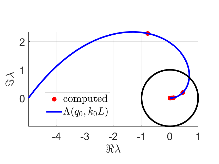
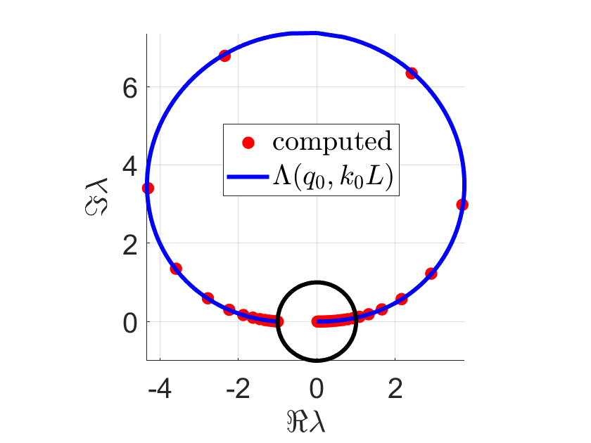
Figure 1. The theoretically predicted set $\Lambda(q_{0},k_{0}L)$ that includes the eigenvalues of $V_{q}(k_{0})$, plotted against the numerically computed eigenvalues. The parameter values are: top, $k_{0}=1$, $L=1$, and $q_{0}=5$; bottom, $k_{0}=50$, $L=1$, and $q_{0}=1$. The reference circle is centered at the origin and has radius one.

Since $\Im\lambda>0$ and since the eigenvalues of $V_{q}(k_{0})$ accumulate precisely at zero, we have

$$\lim_{t\rightarrow 0}\frac{\Re\omega(t)-1}{\Im\omega(t)}=-\infty$$

for

$$\omega(t)=\frac{q_{0}}{s(t)^{2}-1},\quad t\in(0,T(k_{0}L)];$$

here $s(t)$ is given by the above definition of $S_{\pm}(k_{0}L)$. Furthermore, if $\Re\omega(t)<1$ then $(\Re\omega(t)-1)/\Im\omega(t)<0$, while $\Re\omega(t)\geq 1$ implies

$$\frac{1-t^{2}\sinh^{2}k_{0}Lt+\cosh(k_{0}Lt)\sqrt{1-t^{2}\sinh^{2}k_{0}Lt}}{\sinh^{2}k_{0}Lt}\leq\frac{q_{0}}{2};$$

the latter can be seen by rewriting $\Re\omega-1\geq 0$ as

$$((\Re s)^{2}-(\Im s)^{2}-1)((\Re s)^{2}-(\Im s)^{2}-1-q_{0})+4(\Re s)^{2}(\Im s)^{2}\leq 0,$$

and noting that $(\Re s)^{2}-(\Im s)^{2}-1>0$ and $(\Re s)^{2}(\Im s)^{2}>0$. Now since also

$$\frac{1-t^{2}\sinh(k_{0}Lt)^{2}-\cosh(k_{0}Lt)\sqrt{1-t^{2}\sinh(k_{0}Lt)^{2}}}{t\sinh(k_{0}Lt)(\cosh(k_{0}Lt)-\sqrt{1-t^{2}\sinh(k_{0}Lt)^{2}})}$$

$$\leq\frac{1-t^{2}\sinh(k_{0}Lt)^{2}+\cosh(k_{0}Lt)\sqrt{1-t^{2}\sinh(k_{0}Lt)^{2}}}{t\sinh(k_{0}Lt)(\cosh(k_{0}Lt)+\sqrt{1-t^{2}\sinh(k_{0}Lt)^{2}})},$$

we have

$$\frac{\Re\omega(t)-1}{\Im\omega(t)}<\frac{\Re\omega(t)}{\Im\omega(t)}<\frac{1-t^{2}\sinh^{2}k_{0}Lt+\cosh(k_{0}Lt)\sqrt{1-t^{2}\sinh^{2}k_{0}Lt}}{t\sinh(k_{0}Lt)(\cosh k_{0}Lt+\sqrt{1-t^{2}\sinh^{2}k_{0}Lt})},$$

so $\Re\omega(t)\geq 1$ implies

$$\frac{\Re\omega(t)-1}{\Im\omega(t)} <\frac{q_{0}}{2}\frac{\sinh k_{0}Lt}{t(\cosh k_{0}Lt+\sqrt{1-t^{2}\sinh^{2}k_{0}Lt})}\leq\frac{q_{0}}{2}\frac{\tanh k_{0}Lt}{t}$$

$$\leq\frac{q_{0}}{2}\lim_{\tau\searrow 0}\frac{\tanh k_{0}L\tau}{\tau}=\frac{q_{0}k_{0}L}{2},$$

that is, we get a similar estimate on $(\Re\omega(t)-1)/\Im\omega(t)$ as we do on $\|V_{q}(k_{0})\|$. Next, define

(22) $$\xi_{+}=\arctan\sup_{\omega\in\Lambda(q_{0},k_{0}L)}\frac{\Im\left(e^{i\alpha}(1-\omega)\right)}{\Re\left(e^{i\alpha}(1-\omega)\right)}$$

and

(23) $$\xi_{-}=\arctan\inf_{\omega\in\Lambda(q_{0},k_{0}L)}\frac{\Im\left(e^{i\alpha}(1-\omega)\right)}{\Re\left(e^{i\alpha}(1-\omega)\right)}.$$

With $\alpha\in(0,\pi/2)$, $\varepsilon>0$, and $\gamma=\varepsilon e^{i{\alpha}}$, we have $\arg(\gamma(1-\omega))\in[\xi_{-},\xi_{+}]$ for all $\omega\in\Lambda(q_{0},k_{0}L)$, and if

(24) $$\varepsilon<\frac{1}{{1+k_{0}Lq_{0}/2}}\frac{|\tan(2\max\{|\xi_{+}|,|\xi_{-}|\})|}{\tan(\max\{|\xi_{+}|,|\xi_{-}|\})}$$

then $|\gamma(1-\omega)-1|<1$ for all $\omega\in\Lambda(q_{0},k_{0}L)$, and specifically $|\gamma(1-\lambda^{\prime})-1|<1$ for all eigenvalues $\lambda^{\prime}$ of $V_{q}(k_{0})$; the condition (24) can be deduced by requiring $\Im(\gamma(1-\omega))<|\tan(\pi-2\arg(\gamma(1-\omega)))|$ and using $|1-\omega|\leq 1+\|V_{q}(k_{0})\|$. Note that we must choose $\alpha<\pi/2$ rather than $\alpha=\pi/2$ since

$$\frac{\Im(e^{i\alpha}(1-\omega(t)))}{\Re(e^{i\alpha}(1-\omega(t)))}\underset{t\rightarrow 0}{\longrightarrow}\tan\alpha,$$

which for $\alpha=\pi/2$ forces $\xi_{+}=\pi/2$ and thus $\varepsilon<0$. Note furthermore that we can bound (22)–(23) analytically for

$$\alpha=\arctan\frac{1+\frac{k_{0}Lq_{0}}{2}\varepsilon^{\prime}}{\varepsilon^{\prime}-\frac{k_{0}Lq_{0}}{2}},$$

with $\varepsilon^{\prime}>k_{0}Lq_{0}/2$, since

$$-\cot\alpha\leq\frac{\Im\left(e^{i\alpha}(1-\omega)\right)}{\Re\left(e^{i\alpha}(1-\omega)\right)}\leq\tan\alpha,\quad\omega\in\Lambda(q_{0},k_{0}L),\quad\Re\omega\leq 1,$$

since furthermore (recall that $(\Re\omega-1)/\Im\omega<k_{0}Lq_{0}/2<\tan\alpha$)

$$-\frac{\frac{k_{0}Lq_{0}}{2}\tan\alpha+1}{\tan\alpha-\frac{k_{0}Lq_{0}}{2}}\leq\frac{\Im\left(e^{i\alpha}(1-\omega)\right)}{\Re\left(e^{i\alpha}(1-\omega)\right)}<0,\quad\omega\in\Lambda(q_{0},k_{0}L),\quad\Re\omega>1,$$

and finally since

$$-\cot\alpha>-\frac{\frac{k_{0}Lq_{0}}{2}\tan\alpha+1}{\tan\alpha-\frac{k_{0}Lq_{0}}{2}}=-\varepsilon^{\prime}.$$

∎

Remark 3.

A drawback of preconditioning is that, with increasing $k_{0}Lq_{0}$, the acceptable values of $\alpha$ and of $\arctan\varepsilon^{\prime}$ tend to $\pi/2$, and $\varepsilon$ therefore tends to zero. Thus, while the Neumann series remains convergent, the equation

$$(I-M)u=\gamma\psi$$

may be said, especially in a numerical context, to lose information about the operator $V_{q}(k_{0})$ and about the original inhomogeneity $\psi$, as both are multiplied with $\gamma=\varepsilon e^{\i\alpha}$ there.

Remark 4.

Instead of using the bound on $\varepsilon$ stated in Lemma 2, we can estimate $\xi_{+}$ and $\xi_{-}$ from (22)–(23) numerically and arrive at a larger sufficiently small $\varepsilon$ using (24).

We show numerical examples of the use of preconditioning in Section 4.

4. Numerical examples

We here present several numerical examples in dimension one. Fix a positive wavenumber $k_{0}$, obstacle size $L>0$, medium function $q\in L^{2}(]0,L[)$, $q(x)>-1$, and consider the following system for the scattered wave $u(x)$ corresponding to the left excitation $\exp(ik_{0}x)$ in dimension one:

(25) $$\left\{\begin{array}[]{rcl}\psi^{\prime\prime}(x)+k_{0}^{2}(1+q(x))\psi(x)&=&-k_{0}^{2}q(x)\exp(ik_{0}x),\quad x\in]0,L[,\\ -\psi^{\prime}(0)&=&ik_{0}\psi(0),\\ \psi^{\prime}(L)&=&ik_{0}\psi(L).\end{array}\right.$$

The function $G(x,y)=(i/2k_{0})\exp(ik_{0}|x-y|)$, $x,y\in[0,L]$, is the free-space Green’s function associated with the boundary problem (25), since

$$\left\{\begin{array}[]{rcl}(\partial_{y}^{2}+k_{0}^{2})G(x,y)&=&-\delta(x-y),\quad x,y\in]0,L[,\\ -\partial_{y}G(x,0)&=&ik_{0}G(x,0),\quad x\in]0,L[,\\ \partial_{y}G(x,L)&=&ik_{0}G(x,L),\quad x\in[0,L].\end{array}\right.$$

Multiplying the differential equation in (25) with $G(x,y)$ and integrating by parts, we get the Lippmann-Schwinger equation

(26) $$(I-V_{q}(k_{0}))\psi(x)=V_{q}(k_{0})\exp(ik_{0}\cdot)(x),\quad x\in]0,L[,$$

where

$$V_{q}(k_{0})u(x)=\frac{ik_{0}}{2}\int_{y=0}^{L}e^{ik_{0}|x-y|}q(y)u(y)dy,\quad x\in]0,L[.$$

The operator $V_{q}(k_{0}):L^{2}(]0,L[)\rightarrow L^{2}(]0,L[)$ is compact, with norm satisfying

$$\|V_{q}(k_{0})\|^{2}\leq\int_{x=0}^{L}\int_{y=0}^{L}\left|\frac{ik_{0}}{2}e^{ik_{0}|x-y|}q(y)\right|^{2}dydx=\frac{k_{0}^{2}L\|q\|^{2}_{2}}{4}.$$

Now let $q_{0}\in]-1,+\infty[$, and assume that $q|_{]0,L[}\equiv q_{0}$. One can easily prove

$$\mathfrak{H}_{0}=\textrm{Span}\left(V_{q}(k_{0})^{j}e^{ik_{0}\cdot};\;j\in\mathbb{N}\right)=\textrm{Span}\left(V_{1}(k_{0})^{j}e^{ik_{0}\cdot};\;j\in\mathbb{N}\right).$$

On the other hand, since $V_{q}(k_{0})=q_{0}V_{1}(k_{0})$, we have

$$\textrm{Spr}\left((V_{q})_{0}(k_{0})\right)=|q_{0}|\textrm{Spr}\left((V_{1})_{0}(k_{0})\right),$$

where $(V_{q})_{0}(k_{0})$ and $(V_{1})_{0}(k_{0})$ are the restrictions of $V_{q}(k_{0})$ and $V_{1}(k_{0})$, respectively, to the space $\mathfrak{H}_{0}$. Following the proof of Proposition 1, the Born series

$$\sum_{j=1}^{\infty}\left(V_{q}(k_{0})\right)^{j}e^{ik_{0}\cdot}$$

is convergent if and only if $\textrm{Spr}\left((V_{q})_{0}(k_{0})\right)<1$, that is, if and only if

$$|q_{0}|<\frac{1}{\textrm{Spr}\left((V_{1})_{0}(k_{0})\right)}.$$

To illustrate this, we show in Figure 2 two cases of repeated application of $V_{q}(k_{0})$ on the original right-hand side $V_{q}(k_{0})e^{ik_{0}\cdot}$.

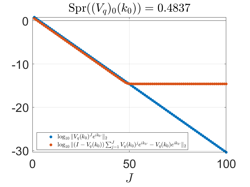
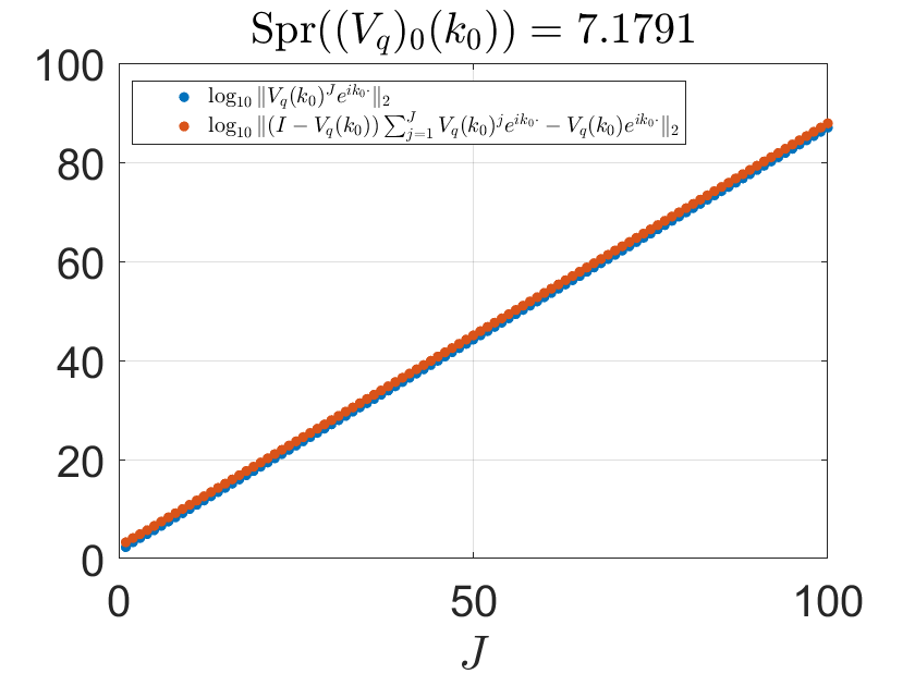
Figure 2. Top: $k_{0}=1$, $L=1$, $q_{0}=1$. Bottom: $k_{0}=50$, $L=1$, $q_{0}=1$.

In the case where Spr$((V_{q})_{0}(k_{0}))<1$, the series $(V_{q}(k_{0})^{J}e^{ik_{0}\cdot})$ converges strongly to zero, while $(I-V_{q}(k_{0}))\sum_{j=1}^{J}V_{q}(k_{0})^{j}e^{ik_{0}\cdot}$ converges strongly to $V_{q}(k_{0})e^{ik_{0}\cdot}$, The second of the two convergence processes plateaus for large values of $J$ due to the effect of numerical errors. In contrast, neither sequence converges in the case where Spr$((V_{q})_{0}(k_{0}))\geq 1$.

Finally, we illustrate Lemma 2 numerically in Figures 3 and 4. We indeed get a convergent Neumann series solution for the case $k_{0}=50$, $L=1$, $q_{0}=1$, albeit the convergence is rather slow.

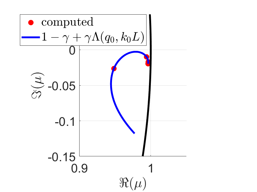
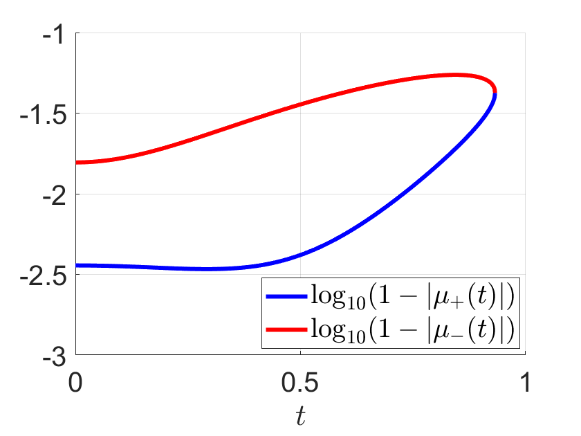
a) $k_{0}$=1, $L=1$, $q_{0}=5$, $\|V_{q}(k_{0})\|=2.4183$, $\varepsilon^{\prime}=5.2$, $\alpha=1.3803$, $\varepsilon=0.02$, $T=0.9320$.

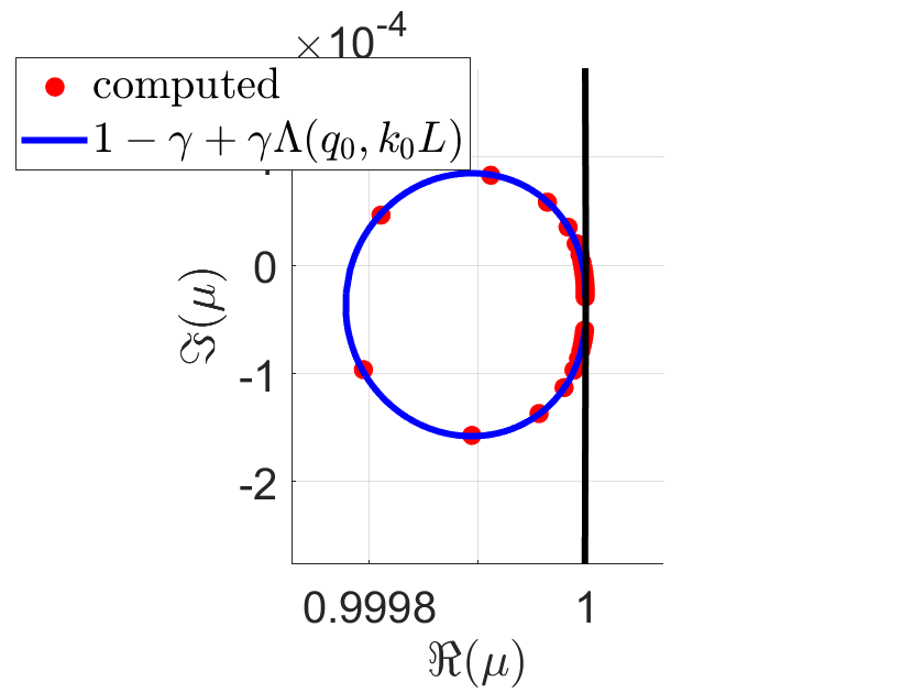
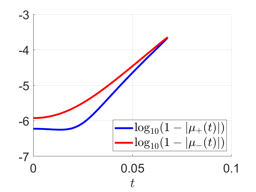
b) $k_{0}=50$, $L=1$, $q_{0}=1$, $\|V_{q}(k_{0})\|=7.1791$, $\varepsilon^{\prime}=50$, $\alpha=1.5508$, $\varepsilon=3\cdot 10^{-5}$, $T=0.0677$.

Figure 3. The original theoretically predicted and numerically computed spectra of $V_{q}(k_{0})$; the transformed curve $\{z=1-\gamma(1-\omega),\,\,\,\omega\in\Lambda(q_{0},k_{0}L)\}\subset\bm{C}$ is included in the unit open disk centered at 1.

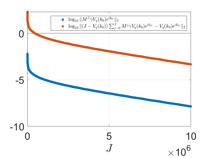
Figure 4. Preconditioning of the equation $(I-V_{q}(k_{0}))u=V_{q}(k_{0})e^{ik_{0}\cdot}$ results in a convergent Neumann series solution. The parameters here are as in Figure 2 (bottom) and Figure 3 b).

References

- [1] H. Ammari, J. Garnier, H. Kang, M. Lim, and K. Solna, Multistatic imaging of extended targets, SIAM J. Imaging Science, 5 (2012), 564–600.
- [2] G. Bao, Y. Chen, and F. Ma, Regularity and stability for the scattering map of a linearized inverse medium problem, J. Math. Anal. Appl., 247 (2000), 255–271.
- [3] S. Arridge, S. Moskow and J. C. Schotland, Inverse Born series for the Calderon problem, Inverse Probl. 28, 035003 (2012).
- [4] P. Bardsley and F. Guevara Vasquez, Restarted inverse Born series for the Schrödinger problem with discrete internal measurements, Inverse Probl. 30, 045014 (2014).
- [5] H. W. Engl and M. Z. Nashed. Generalized Inverses of Random Linear Operators in Banach Spaces. Journal of Mathematical Analysis and Applications, 83, 582–610 (1981)
- [6] B. Osting and M. I. Weinstein. Long-lived Scattering Resonances and Bragg Structures. SIAM Journal on Applied Mathematics, 73(2) (2013)
- [7] A. McIntosh and M. Mitrea. Clifford Algebras and Maxwell’s Equations in Lipschitz Domains. Mathematical Methods in the Applied Sciences, 22, 1599–1620 (1999)
- [8] C.-C. Chou, J. Yao, and D. J. Kouri. Volterra inverse scattering series method for one-dimensional quantum barrier scattering. International Journal of Quantum Chemistry, 117:e25403 (2017)
- [9] R. G. Newton. Scattering Theory of Waves and Particles, Second Edition, Springer, 1982.
- [10] G. Bao and F. Triki. Stability for the multifrequency inverse medium problem. Journal of Differential Equations, 269(9), 7106-7128 (2020)
- [11] G. Bao and F. Triki. Error estimates for the recursive linearization of inverse medium problems. J. Comput. Math. 28, No. 6, 725–744
- [12] M. Karamehmedović and K. Linder-Steinlein. Spectral properties of radiation for the Helmholtz equation with a random coefficient. In review.’
- [13] K. Kilgore, S. Moskow and J. C. Schotland, Convergence of the Born and inverse Born series for electromagnetic scattering, Applicable Analysis 96, 1737 (2017).
- [14] K. Kilgore, S. Moskow and J. C. Schotland, Inverse Born series for scalar waves, J. Computational Math. 30, 601 (2012).
- [15] A. Louis, Approximate inverse for linear and some nonlinear problems, Inverse Probl. 12, 175 (1996).
- [16] M. Machida and J. C. Schotland, Inverse Born series for the radiative transport equation, Inverse Probl. 31, 095009 (2015).
- [17] V. Markel, J. A. O’Sullivan and J. C. Schotland, Inverse problem in optical diffusion tomography.IV nonlinear inversion formulas, J. Opt. Soc. Am A, 20, 903 (2003).
- [18] T. Kato. Perturbation theory for linear operators. Vol. 132. Springer Science & Business Media, 2013.
- [19] A. Lechleiter, K. S. Kazimierski and M. Karamehmedović. Tikhonov regularization in applied to inverse medium scattering. Inverse Problems 29, 075003 (2013)
- [20] N. Suzuki. On the Convergence of Neumann Series in Banach Space. Mathematische Annalen 220, 143–146 (1976)
- [21] G. Osnabrugge, S. Leedumrongwatthanakun and I. M. Vellekoop. A convergent Born series for solving the inhomogeneous Helmholtz equation in arbitrarily large media. Journal of Computational Physics 322, 113–124 (2016)
- [22] H. Lopez-Menchon, J. M. Rius, A. Heldring and E. Ubeda. Acceleration of Born Series by Change of Variables. IEEE Transactions on Antennas and Propagation 69(9), 5750–5760 (2021)
- [23] S. Moskow, and J. C. Schotland, Numerical studies of the inverse born series for diffuse waves, Inverse Problems, 25 (2009) 095007-25.
- [24] S. Moskow, and J. C. Schotland, Convergence and stability of the inverse scattering series for diffuse waves, Inverse Problems, 24 (2008) 065005-2
- [25] S. Moskow, and J. C. Schotland, Inverse Born Series, in The Radon Transform: The First 100 Years and Beyond, edited by R. Ramlau and O. Scherzer (De Gruyter, 2019)
- [26] G. Panasyuk, V. A. Markel, P. S. Carney and J. C. Schotland, Nonlinear inverse scattering and three dimensional near-field optical imaging, App. Phys. Lett. 89, 221116 (2006)
- [27] C. Brezinski. Convergence acceleration during the 20th century. Journal of Computational and Applied Mathematics 122, 1–21 (2000)
- [28] R. E. Kleinman and G. F. Roach. Iterative solutions of boundary integral equations in acoustics. Proc. R. Soc. Lond. A 417, 45–57 (1988)
- [29] R. E. Kleinman, G. F. Roach, L. S. Schuetz, and J. Shirron. An iterative solution to acoustic scattering by rigid objects. J. Acoust. Soc. Am. 84(1), 385 (1988)
- [30] R. E. Kleinman, G. F. Roach and P. M. van den Berg. Convergent Born series for large refractive indices. Journal of The Optical Society of America A 7(5), 890–897 (1990)
- [31] M. E. Taylor. Partial Differential Equations I: Basic Theory, Second Edition, Springer, 2011
- [32] D. Colton and R. Kress. Inverse Acoustic and Electromagnetic Scattering Theory, Fourth Edition, Springer, 2019