Lifted Sequential Planning with Lazy Constraint Generation Solvers

Abstract

This paper studies the possibilities made open by the use of Lazy Clause Generation (LCG) based approaches to Constraint Programming (CP) for tackling sequential classical planning. We propose a novel CP model based on seminal ideas on so-called lifted causal encodings for planning as satisfiability, that does not require grounding, as choosing groundings for functions and action schemas becomes an integral part of the problem of designing valid plans. This encoding does not require encoding frame axioms, and does not explicitly represent states as decision variables for every plan step. We also present a propagator procedure that illustrates the possibilities of LCG to widen the kind of inference methods considered to be feasible in planning as (iterated) CSP solving. We test encodings and propagators over classic IPC and recently proposed benchmarks for lifted planning, and report that for planning problem instances requiring fewer plan steps our methods compare very well with the state-of-the-art in optimal sequential planning.

1 Introduction

One of the most significant advances in classical planning was the realisation of Green’s [18] vision for theorem proving as a framework for general problem solving, via the ground-breaking seminal work of H. Kautz and B. Selman [29, 28]. Putting together the insights of Blum and Furst [3], where planning becomes the problem of analysing whether goal states are reachable in a suitably defined graph, with space efficient solutions to the frame problem formulated in the Situation Calculus [32, 19], Kautz & Selman showed that formulating planning problems in terms of satisfiability of Conjunctive Normal Form (CNF) formulas was feasible and, at the time, highly scalable. Attention to planning as satisfiability has been somewhat eclipsed since then with the development of planning algorithms based on direct, but lazy, incremental heuristic search over transition systems [4, 23, 21, 38, 51]. Yet deep theoretical connections exist between planning as satisfiability and as heuristic search [15, 40] questioning [41, 50] perceptions of either approach as being parallel or mutually exclusive.

Like R. Frost’s traveller in the woods this paper finds its way back to a crossroads in the development and study of approaches to planning as satisfiability. One way is that of the so-called GraphPlan encodings (linear and parallel), the other being that of so-called causal encodings (ground and lifted) invented by Kautz, McAllester and Selman (KMS) [28]. Unlike Frost’s poem though, lifted causal encodings are clearly an approach seldom followed in the literature in automated planning. Inspired by the formulation of nonlinear or partially-ordered planning of McAllester and Rosenblitt [31], these encodings have polynomial size over the lower bound on the number of plan steps in feasible plans. Importantly too, they do away entirely with the need for explanatory frame axioms. Yet these very desirable properties follow from the premise of not having to ground actions and predicates first, as otherwise the unavoidable exponential blow outs obliterate any practical differences with GraphPlan encodings.

In this paper we realize this potential by tapping into the power of Lazy Clause Generation (LCG) [35], a ground-breaking technology that unifies propositional satisfiability (SAT) and Constraint Programming (CP), and allows representing implicitly large tracts of complex systems of constraints by suitably defined inference procedures, or propagators. These lazily generate new constraints to record violations by assignments to decision variables, and propagate information following from the consistency of assignments and constraints in order to tighten the domains of variables. This, in addition to very sophisticated and performant modeling tools and solvers [37], provide us the foundations to develop scalable planners that follow the path laid by KMS lifted causal encodings. We have found these planners to clearly outperform state-of-the-art optimal planning algorithms on benchmarks designed to be hard to ground [7], while standing their ground on the IPC benchmarks.

Paper Overview. We start the paper with a precise formulation of the kind of planning problems of interest to us and their solutions. We then introduce a formalism to describe the structure of states and actions that is based on Functional STRIPS [13]. We assume that all atoms in precondition and effects are equality atoms over suitably defined function symbols and constant terms. These ground domain theories are then lifted [31]. With these preliminaries in place, we introduce our encoding, for which we prove validity and provide a characterisation of its complexity. After that, we explain how we leverage state-of-the-art CP solvers to implement efficiently our encoding. We then present a method to do a concise transformation of planning instances represented in PDDL to FSTRIPS. We end with an evaluation of several planners built on top of our encoding and propagators, along with a brief analysis of related work and a discussion of the significance and potential of this research.

2 Formulation of Planning Problems

A problem planning instance (PPI) is given by a tuple $P=(S,A,\to,s_{0},S_{G})$ where $S$ and $A$ are finite sets of states and actions, $\to$ $\subset$ $S\times A\times S$ is the transition relation, where $s\to_{a}s^{\prime}$ indicates that $s^{\prime}$ is reachable from $s$ via $a$, $s_{0}\in S$ is the initial state and $S_{G}\subset S$ is the set of designated goal states. We say that a PPI admits a trajectory $\sigma=s_{0},a_{1},s_{1},\ldots,s_{i-1},a_{i},s_{i}$ iff $s_{i-1}$ $\to_{a_{i}}$ $s_{i}$ for every $i>0$. In this paper the notion of planning problems is that of optimization problems where we seek sequences $\sigma$ $=$ $s_{0},a_{1},s_{1},\ldots,s_{k-1},a_{k},s_{k}$, that minimize $\mathrm{length}(\sigma):=k$, and satisfies $s_{k}\in S_{G}$. The set of $\sigma$ sequences that satisfy $s_{k}\in S_{G}$ is referred to as the set of valid plans $\Pi_{P}$. The optimal cost of $P$ is thus $c^{*}:=\min_{\sigma\in\Pi_{P}}\mathrm{length}(\sigma)$. When $\Pi_{P}=\emptyset$, we say that $P$ is infeasible and optimal cost is $c^{*}=\infty$. We observe that $|S|-1$ is a trivial upper bound on $c^{*}$ when $\Pi_{P}\neq\emptyset$. Non-trivial, feasibly computable upper bounds are known [1] but only for PPIs with special structure.

2.1 Factored Planning Problems

A long recognised and adopted strategy to deal with large $|S|$ is that of factoring states and actions in PPIs as a preliminary step to develop algorithms that can deal with large scale problems [36, 2]. We now present an account of FSTRIPS, a formalism to define such factorings, where a domain theory expresses assumptions on the structure of states and actions [12, Section 2.1].

A PPI $P$ in Functional Strips is defined over a many-sorted first order logic theory with equality, which we denote as ${\cal L}(P)=(T,\Phi,\Pi)$. The constituents of such a theory capture relevant properties of and relations between objects, and provide the basic building blocks to factorize states $s\in S$. $T$ is a finite non-empty set of finite sets called types, or sorts, with a possibly infinite set of variables $x_{1}^{t}$, $x_{2}^{t}$, $\ldots$ for each type $t\in T$. The universe is the set $U=\cup_{t\in T}t$. $\Phi$ is a set of function symbols $f\in\Phi$, each of which is said to have a domain $\mathrm{Dom}_{f}\subset t_{1}\times\dots t_{i}\times\times t_{d_{f}}$ where $t_{i}\in T$, and a range $\mathrm{Co}_{f}$ $\in$ $T$. $\Pi$ is a set of relation symbols. In this paper, $\Pi$ contains the standard relations of arithmetic e.g. “$<$”, “$\leq$”, “$>$”, “$\geq$ ” in addition to equality “$=$”. Some PPIs may specify as well domain specific relations, along with their denotation, in addition to the former standard ones. We denote the maximum function arity of the domain, $\max_{f\in\Phi}d_{f}$, as $K_{f}$. States $s\in S$ in a Fstrips problem $P$ are semantic structures that set the interpretation of formulas over ${\cal L}(P)$ with fixed universe $U$. Thus each $s$ contains the graph [5] of each function $f\in\Phi$, providing the denotation for functional terms $f(\bar{t})$, where $\bar{t}\in\mathrm{Dom}_{f}$. We note that $S(P)$ is a finite set since types $t\in T$ are finite sets too.

The transition relation $\to$ is specified via suitably defined action schemas $\alpha\in Act$. $\alpha$ is a non-logical symbol such that $\alpha\not\in\Phi\cup\Pi$. Actions $\alpha(\bar{x})$ capture sets of transitions in $\to$ parametrized by a tuple of typed variables $\bar{x}=(x_{1}^{t_{1}},\ldots,x_{d_{\alpha}}^{t_{d_{\alpha}}})$. $\tau(\alpha)$ denotes the tuple of types of parameters of $\alpha$, $\tau(\alpha)=(t_{1},\ldots,t_{d_{\alpha}})$. For each action schema $\alpha(\bar{x})$ we are given ${\rm Phys.\leavevmode\nobreak\ Rev.\leavevmode\nobreak\ E}{\alpha}(\bar{x})$ a precondition formula over ${\cal L}(P)$ and variables $\bar{x}$. In this paper we consider a fragment of the formulas considered by [12], defined by the following grammar in Backus-Naur form

$${\rm Phys.\leavevmode\nobreak\ Rev.\leavevmode\nobreak\ E}{\alpha}(\bar{x})\coloneqq\top\,\mid\,\bigwedge_{i=1}^{card({\rm Phys.\leavevmode\nobreak\ Rev.\leavevmode\nobreak\ E}{\alpha})}f_{i}(\bar{y}_{i})=z_{i}$$ (1)

where $\top$ is the tautology, $card({\rm Phys.\leavevmode\nobreak\ Rev.\leavevmode\nobreak\ E}{\alpha})$ denotes the number of equality atoms in the formula ${\rm Phys.\leavevmode\nobreak\ Rev.\leavevmode\nobreak\ E}{\alpha}$, $\bar{y}_{i}\subset\bar{x}$, and $z_{i}\in U$. Additionally, we are given an effect formula $\mathrm{Eff}_{\alpha}$ of the form

$$\mathrm{Eff}_{\alpha}(\bar{x})\coloneqq\bigwedge_{j=1}^{card({\mathrm{Eff}_{\alpha}})}f_{j}(\bar{y}_{j})=z_{j}$$ (2)

where $card(\mathrm{Eff}_{\alpha})$ denotes the number of equality atoms in the formula $\mathrm{Eff}_{\alpha}$, $\bar{y}_{j}\subset\bar{x}$ and $z_{i}\in U$.

We now explain the FSTRIPS representation for the visitall problem domain from the IPCs [26] in which an agent must visit all the cells in an $n\times n$ square grid starting from the center of the grid. In Visitall, we only have one type, $T:=\{C\}$, where $C$ is a set of cells in the grid, the set of function symbols is $\Phi:=\{at,visited\}$, and it has a domain specific relation $\Pi:=\{connected\}$. It has one action schema move which allows the agent to move between two connected cells of the grid, thus, $Act=\{move\}$. The move schema takes two parameters which we denote by $\bar{x}:=(x_{1},x_{2})$, where $x_{1}$ is the current position of the agent and $x_{2}$ is the target position. The precondition and effect formulas of move are defined as follows

$${\rm Phys.\leavevmode\nobreak\ Rev.\leavevmode\nobreak\ E}{\emph{move}}(\bar{x}) \coloneqq at()=x_{1}\land connected(x_{1},x_{2})=\top$$ (3a)

$$\mathrm{Eff}_{\emph{move}}(\bar{x}) \coloneqq at()=x_{2}\land visited(x_{2})=\top$$ (3b)

The goal condition of visitall requires the agent to visit all cells in $C$

$$Goal_{\emph{move}}\coloneqq\bigwedge_{c\in C}visited(c)=\top$$ (4)

A set of action schemas $Act$ is systematic [31, 43] for a PPI $P$ if and only if, for every $(s,a,s^{\prime})\in\to$ there is an action schema $\alpha(\bar{x})$ such that there exists a vector $\bar{v}\in t_{1}\times\dots\times t_{d_{\alpha}}$ and the following conditions hold:

$$s \models{\rm Phys.\leavevmode\nobreak\ Rev.\leavevmode\nobreak\ E}{\alpha}(\bar{x})/\bar{v}$$ (5a)

$$s^{\prime} \models\mathrm{Eff}_{\alpha}(\bar{x})/\bar{v}$$ (5b)

$$s^{\prime} \models g(\bar{v})=w,\,\text{when}\leavevmode\nobreak\ s\models g(\bar{v})=w\land\not\exists w\textquoteright,\mathrm{Eff}_{\alpha}(\bar{x})/\bar{v}\models g(\bar{v})=w\textquoteright$$ (5c)

where $\varphi(\bar{x})/\bar{v}$ is the (ground) formula that results from replacing every occurrence of $x_{i}\in\bar{x}$ by that of $v_{i}\in\bar{v}$. The satisfiability relation in (5a)–(5c) is defined in a standard way [12]. In words, a set of action schemas $Act$ is systematic whenever these capture every possible reachability (or accessibility) relation between states $s$ and $s^{\prime}$. We note that one action schema $\alpha(\bar{x})$ can satisfy the above for many $(s_{1},a_{1},s_{1}^{\prime})$, $(s_{2},a_{2},s_{2}^{\prime})$, …, each of these tuples providing the semantics of ground action $\alpha(\bar{v})$. In this paper we further assume that action schemas do not change the denotation of any symbol in $\Pi$ (see section 5 for a discussion of their treatment in our encoding).

We denote the maximal arity of action schemas in $Act$ as $K_{\alpha}=\max_{\alpha\in Act}d_{\alpha}$. The maximal number of equality atoms in precondition formulas is written as $K_{\mathrm{pre}}=\max_{\alpha\in Act}card({\rm Phys.\leavevmode\nobreak\ Rev.\leavevmode\nobreak\ E}{\alpha})$ (resp. $K_{\mathrm{eff}}=\max_{\alpha\in Act}card(\mathrm{Eff}_{\alpha})$ for effects).

3 Planning as Satisfiability

The approach known as planning as satisfiability [29] proceeds by considering a sequence of instances for a related decision problem, that of plan existence. We state the latter simply as follows: given some PPI $P$ and parameter $N_{\pi}$, with actions and states defined in terms of some domain theory, the task is to prove that a feasible trajectory $\sigma$ exists such that $\mathrm{length}(\sigma)=N_{\pi}$, or alternatively, certify that no such $\sigma$ exists. The classic algorithm for optimal planning in this framework thus considers the sequence of CSPs $T_{P,n_{0}}$, $T_{P,n_{1}}$, $\ldots$, $T_{P,n_{k}}$, $\ldots$ each of these a reduction of the plan existence problem for $P$ and $N_{\pi}=n_{k}$ into that of the satisfiability of a CSP $T_{P,n_{k}}$ with suitably defined decision variables and constraints. The sequence of natural numbers $n_{0},n_{1},\ldots,n_{k},\ldots$ is typically, but not necessarily [48], defined as $n_{0}$ $=$ $0$, $n_{1}$ $=$ $1$, and so on. When defined in this manner, as soon as $T_{P,n_{k}}$ is satisfiable, we have proven that $c^{*}=n_{k}$. Scalable certification of infeasibility in this framework has been an open problem until recently [8], yet still remains challenging.

4 Lifted Causal CP Model

Symbol	Description
$act_{i}$	Action assigned to slot $i$, $i=1,\ldots,N_{\pi}$
$active_{ik}$	Pin is active
$arg_{ij}$	Value of $j$-th argument of slot $i$, $j=1,\ldots,K_{\alpha}$
$in_{ik}$	$k$-th input pin data of slot $i$
$out_{il}$	$l$-th output pin data of slot $i$
$spt_{jk}$	Output pin supporting $k$-th input pin of slot $j$

Table 1: Quick reference table for the decision variables in the model. $N_{\pi}$ is the number of slots, $K_{\alpha}$ is the (constant) maximal number of arguments in any action schema $\alpha\in Act$.

We start by giving a high-level account of our proposed encoding of CSPs $T_{P,N_{\pi}}$ and explain the roles played by the decision variables in Table 1. Central to our encoding is the notion of plan step or slot, of which we have one for each action in a plan. In contrast with the causal encoding of KMS, slots are totally ordered thus greatly simplifying the definition of persistence that we use to deal with the frame axioms. To each slot exactly one action schema $\alpha\in Act$ needs to be assigned (variables $act_{i}$), which in turn restricts choices on the possible values for the arguments (variables $arg_{ij}$) of the schema $\alpha$ as per $\tau(\alpha)$. The assignments to the variables $act_{i}$ and $arg_{ij}$ determine the choices of input and output pins for a slot. A pin is a vector of decision variables which we use to represent equality atoms $f(\bar{y})=z$. These variables choose the function symbol $f$, terms (constants in $U$) $\bar{y}$ (a vector) and $z$. Input pins of slot $i$ thus encode the equality atoms in ${\rm Phys.\leavevmode\nobreak\ Rev.\leavevmode\nobreak\ E}{\alpha}(\bar{x})/\bar{v}$ required to be true in state $s_{i-1}$, and output pins the atoms in $\mathrm{Eff}_{\alpha}(\bar{x})/\bar{v}$ required to be true in $s_{i}$, where $\alpha(\bar{v})$ is the ground action selected by the assigned schema and (possibly partially) assigned values to arguments. These dependencies between the variables of a slot are depicted in Figure 1(a), and Figure 1(b) illustrates the active constraints between variables when the move action schema is chosen at slot $i$ in the visitall problem domain. The move schema has two arguments representing the current position and the target position of an agent in an $n\times n$ grid. Thus, when $act_{i}=\emph{move}$, we require that $arg_{i1}\in C$ and $arg_{i2}\in C$, the input pin $in_{i1}$ is assigned the function symbol $at$ and the variable $y_{i1}$ holds an equality relation with $arg_{i1}$.

We note that we create up front variables for arguments and pins following from $K_{\alpha}$, $K_{f}$, $K_{\mathrm{pre}}$ and $K_{\mathrm{eff}}$, all constants given by the data in an instance $P$. For a given slot $i$, argument variables $arg_{ij}$ that are not used by the schema assigned are set to a special $\mathrm{null}$ constant. To disable pins not needed to represent atoms in preconditions or effect formulas we have a Boolean variable $active_{ik}$ that indicates if they are being used. Finally, variables $spt_{jk}$ allow choosing what output pin is supporting a given input pin. These variables allow encoding causal links [31] without referring explicitly to atoms.

4.1 Variables and Constraints

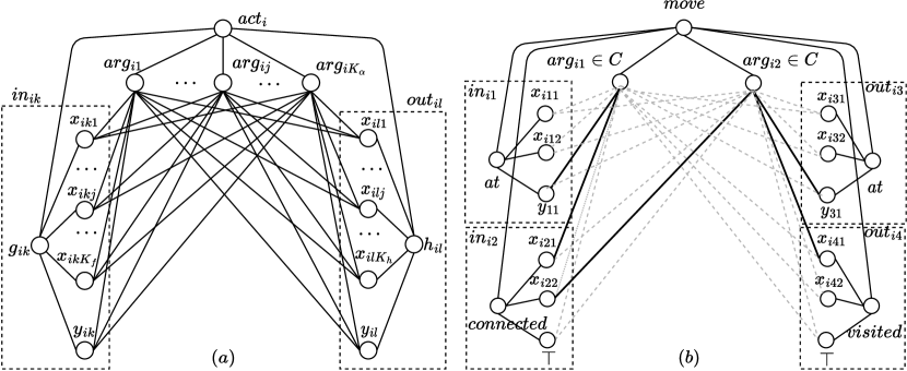
Figure 1: $(a)$ Constraint graph depicting dependencies between the decision variables to model slots (plan steps). There is one vertex for every decision variable, and there is an edge between two variables whenever they appear together in the definition of at least one constraint. $(b)$ Active constraints when the move action schema is chosen in visitall.

We now give a formal and precise account of the variables and constraints in the model. Let $N_{\pi}$ be the maximal number of slots in a valid plan. For every slot $i=1,\ldots,N_{\pi}$ we have integer variables $act_{i}\in[Act]$ to choose the action schema $\alpha\in Act$ assigned to it. Argument variables $arg_{ij}$ select the values of the variables introduced by lifting, and their domains correspond to the types $\tau_{j}(\alpha)$, whenever $act_{i}=\alpha$

$$(act_{i}=\alpha)\rightarrow arg_{ij}\in[\tau_{j}(\alpha)],\,j=1,\ldots,d_{\alpha}$$ (6)

The choice of action schema assigned to a slot restricts the choices of (ground) precondition and effect formulas. As introduced above, the input and output pins of a slot $i$ are the vectors of decision variables that select function symbols, arguments and values $in_{ik}$ $:=$ $(g_{ik},x_{ik1},\ldots,x_{ik\bar{N}_{f}},y_{ik})$ and $out_{il}$ $:=$ $(h_{il},x_{il1},\ldots,x_{il\bar{N}_{f}},y_{il})$. Consistency of schema, preconditions and effects assigned to slot $i$ is enforced by

$$(act_{i}=\alpha) \rightarrow(g_{ik}=f_{k})\land\mathrm{bind}(f_{k},\bar{x}_{ik},y_{ik},\overline{arg}_{i})$$ (7a)

$$(act_{i}=\alpha) \rightarrow(h_{il}=f_{l})\land\mathrm{bind}(f_{l},\bar{x}_{il},y_{il},\overline{arg}_{i})$$ (7b)

for $k=1,\ldots,card({\rm Phys.\leavevmode\nobreak\ Rev.\leavevmode\nobreak\ E}{\alpha})$ and $l=1,\ldots,card(\mathrm{Eff}_{\alpha})$. $\overline{arg}_{i}$ is the vector of argument variables for slot $i$. The predicate $\mathrm{bind}$ in (7a) and (7b) ensures that subterms $\bar{x}$ and $y$ of equality atoms in preconditions and effects are consistent with the definition of schema $\alpha$, expanding into the following

$$\bigwedge_{j=1}^{d_{f}}\bigg{(}\bigvee_{j_{2}=1}^{K_{\alpha}}(x_{j}={arg}_{ij_{2}})\bigg{)}\land\bigvee_{j_{2}=1}^{K_{\alpha}}(y={arg}_{ij_{2}})$$ (8)

The dependencies induced by constraints (6)–(8) are depicted in Figure 1,

States are represented implicitly in our model, and in order to ensure that no change on the initial state $s_{0}$ is allowed without an event in the plan that explains any changes we rely on the notion of causal consistency or persistence

Definition 4.1.

Let $f(\bar{x})$ be a functional term $f\in\Phi$ and $y$ a valid value in $\mathrm{Co}_{f}$. We say that the truth of atom $f(\bar{x})=y$ persists between slots $i$ and $j$, $0\leq i<j\leq N_{\pi}$, if (1) $f:\bar{x}\mapsto_{s_{i}}y$, and (2) for every slot $j^{\prime}$, $i<j^{\prime}<j$, there is no pin $out_{j^{\prime}l}=(h_{j^{\prime}l},\bar{x}_{j^{\prime}l},y_{j^{\prime}l})$ such that $h_{j^{\prime}l}=f$, $\bar{x}_{j^{\prime}l}=\bar{x}$, and $y_{j^{\prime}l}\neq y$.

This ensures that states $s_{j}$ are given either by 1) function and value assignments in the initial state $s_{0}$ that have persisted through (ground) actions $a_{i}$ encoded in slots $i$, $0$ $<$ $i$ $<$ $j$, or 2) an assignment made by some action $a_{i}$ encoded in some slot $i$, $0$ $<$ $i$ $<$ $j$, that has persisted through the actions $a_{j^{\prime}}$ encoded by slots $j^{\prime}$, $i$ $<$ $j^{\prime}$ $<$ $j$. For example, in visitall, an atom $at()=c_{1}$ in the intial state, where $c_{1}$ is the initial position of the agent, is said to have persisted until slot $3$ iff the atom holds at slot $1$ and $2$.

The many possible cause-and-effect relations between output and input pins that may justify the causal consistency of a plan are modelled via so-called (causal) support variables, $spt_{jk}$ $\in$ $\big{(}[0,j-1]\times[1,K_{\mathrm{eff}}]\big{)}\cup\{\mathrm{null}\}$, for each slot $0$ $<$ $j$ $\leq$ $N_{\pi}$ and input pin $1$ $\leq$ $k$ $\leq$ $K_{\mathrm{pre}}$. The domain of these variables is the set of two-dimensional vectors whose first element is the index of the slot $i$ and the second the index $l$ of the output pin supporting $in_{jk}$, plus a dummy vector $\mathrm{null}$ that indicates that input pin $in_{jk}$ does not have a causal support assigned. The following constraints enforce that every active pin has a matching supporting one

$$spt_{jk}=\mathrm{null} \rightarrow\,\neg active_{jk}$$ (9a)

$$spt_{jk}=(i,l) \rightarrow\,out_{il}=in_{jk}$$ (9b)

$$spt_{jk}=(i,l) \rightarrow\,\bigwedge_{i<j^{\prime}<j}\mathrm{persists}(out_{j^{\prime}l},in_{jk})$$ (9c)

for each $1$ $\leq$ $j$ $\leq$ $N_{\pi}$ and $0$ $\leq$ $i$ $<$ $j$. Constraint (9a) excuses input pins that are inactive from having a causally supporting output pin. Constraint (9b) ensures that the values for functions, domain and valuation set by pins $in_{jk}$ and $out_{il}$ are matching. Constraint (9c) encodes the requirement of causal supports to not be interfered by any ground action set for intermediate slots $i<j^{\prime}<j$. $\mathrm{persists}(out_{il},in_{jk})$ in constraint (9c) expands into the formula

$$(h_{il}\neq g_{jk})\lor(\bar{x}_{il}\neq\bar{x}_{jk})\lor(y_{il}=y_{jk})$$ (10)

In the specific case of visitall, the constraints (9) and (10) impose additional constraints on the input and output pin variables than the ones depicted in Figure 1(b), thus, restricting the choices of $act_{i}$ and $\overline{arg}_{i}$ as well. For example, if $spt_{31}=(1,3)$, then the constraint (9b) requires that the assignment to $out_{13}:=(at,y_{13})$ matches that of $in_{31}:=(at,y_{31})$, i.e. $y_{13}=y_{31}$, and the constraints (9c) and (10) ensure that the assignment to $out_{13}$ persists through slot $2$, i.e. the (ground) action $a_{2}$ does not affect the interpretation of $at$. It is easy to see that when $spt_{31}=(1,3)$, the choice of $y_{13}$ in turn affects $arg_{31}$ since $arg_{31}$ holds an equality relation with $y_{31}$.

Additionally, whenever we assign action schemas $\alpha$ to slots $i$ we mark input and output pins as being active

$$act_{i}=\alpha\rightarrow active_{ik},\,act_{i}=\alpha\rightarrow\neg active_{ik^{\prime}}$$ (11a)

$$act_{i}=\alpha\rightarrow active_{il},\,act_{i}=\alpha\rightarrow\neg active_{il^{\prime}}$$ (11b)

with indices ranging as follows: $1$ $\leq$ $k$ $\leq$ $card({\rm Phys.\leavevmode\nobreak\ Rev.\leavevmode\nobreak\ E}{\alpha})$, $card({\rm Phys.\leavevmode\nobreak\ Rev.\leavevmode\nobreak\ E}{\alpha})$ $<$ $k^{\prime}$ $\leq$ $K_{\mathrm{pre}}$, $1$ $\leq$ $l$ $\leq$ $card(\mathrm{Eff}_{\alpha})$, $card(\mathrm{Eff}_{\alpha})$ $<$ $l^{\prime}$ $\leq$ $K_{\mathrm{eff}}$. Initial and goal states are accounted for in the following way. To model the initial state, we define slot $0$ to consist exclusively of a set of (output) pins $out_{0l}$ where $l$ ranges over the indexing of the set

$${\cal F}:=\bigcup_{f\in\Phi}\mathrm{Dom}_{f}$$ (12)

and each pin is set as per constraints, for each $l\in[{\cal F}]$

$$out_{0l}=(f_{l},\bar{x}_{l},y)$$ (13)

and $y\in\mathrm{Co}_{f}$ such that $f_{l}:\bar{x}_{l}\mapsto_{s_{0}}y$. Goal states are modelled too by having the slot $N_{\pi}$ to have special structure, in this case by only having input pins $in_{N_{\pi}k}$ with $k$ ranging over the indexing of the set of equality atoms $\varphi_{k}\equiv f_{k}(\bar{x}_{k})=y_{k}$ in the goal formula

$$\bigwedge_{\varphi_{k}\in Goal}in_{N_{\pi}k}=(f_{k},\bar{x}_{k},y_{k})\land active_{N_{\pi}k}$$ (14)

4.2 Analysis: Systematicity and Complexity

We first establish as fact that our encoding is systematic  [31].

Theorem 4.2 (Systematicity).

Let $T_{P,N_{\pi}}$ $=$ $({\cal X}$, ${\cal C})$ be the CSP given by the decision variables ${\cal X}$ in Table 1 and set of constraints ${\cal C}$ (6)–(14), for some suitable choice of $N_{\pi}$. There exists an assignment $\xi$ onto variables ${\cal X}$ that satisfies every constraint in ${\cal C}$ if an only if there exists a feasible solution $\sigma$ to the PPI $P$, whose actions are given by slots, argument, input and output pin variables values.

Proof 4.3.

See B.1.

Giving bounds on the number of variables generated for a CP model is not as informative as doing so for CNF formulas due to the advanced pre-solving techniques that state-of-the-art CP solvers employ [37], that may introduce auxiliary Boolean variables and eliminate variables whose values can be determined without searching. Assuming that no such transformations are applied to the CSP, the set of $spt_{jk}$ variables and their domain constraints, which are required to be encoded explicitly by LCG solvers [35], is the largest and is $O(N_{\pi}^{2}K_{max})$ where $K_{max}$ $=$ $\max$ $\{$ $K_{\mathrm{pre}}$, $K_{\mathrm{eff}}$ $\}$. In the IPC benchmarks, this results often in just a quadratic rate of growth as $K_{max}$ is usually much smaller than $N_{\pi}$ for optimal plans. Yet, as we will see in our Evaluation, this is not always the case, and we get cubic rates.

5 Programming the Model with CpSat

To implement the CP model introduced in the previous section we have used the LCG solver bundled in Google’s Or-Tools package, CpSat [37]. At the time of writing this, CpSat is the state-of-the-art LCG solver as adjudicated by the latest results of the Minizinc challenge [49]. A key feature of CpSat we rely on is the extensive support for different variants of so-called $\mathrm{element}(\cdot)$ constraints [24]. These constraints implement variable indexing, a key modeling feature in CP, and correspond with the statement $\bar{v}_{x}=z$, that reads as “the element at position $x$ of vector $\bar{v}$ must be equal to $z$”. The power of these constraints lies in the possibility of elements of $\bar{v}=(v_{1},\ldots,v_{m})$, $x$ and $z$ being all decision variables. We write $\mathrm{element}(\cdot)$ constraints using Hooker’s [24] notation

$$\mathrm{element}(x,z\mid\bar{v})$$ (15a)

$$\mathrm{element}((x_{1},x_{2}),z\mid V)$$ (15b)

where (15a) implements the statement $\bar{v}_{x}=z$, and (15b) implements $V(x_{1},x_{2})=z$ that reads as “the element of matrix $V$ at coordinates $x_{1},x_{2}$ must be equal to $z$”. $x$, $x_{1}$ and $x_{2}$ are thus index variables that locate one decision variable within a collection.

In our implementation, the action assigned to slot $i$, $act_{i}$ is an index variable, which depends on the data assigned to input and output pins as per constraints  (7) and (8). Both of these constraints can be encoded compactly using (15a)

$$\mathrm{element}(act_{i},g_{ik}\mid(f_{1},f_{2},\ldots,f_{j},\ldots,f_{|Act|}))$$ (16a)

$$\mathrm{element}(act_{i},x_{ikl}\mid(\nu_{1},\nu_{2},\ldots,\nu_{j}\ldots,\nu_{|Act|}))$$ (16b)

$$\mathrm{element}(act_{i},y_{ik}\mid(\mu_{1},\mu_{2},\ldots,\mu_{j}\ldots,\mu_{|Act|}))$$ (16c)

where $f_{j}$ is a function symbol, $\nu_{j}$ and $\mu_{j}$ are the argument variables of slot $i$ or constants that are consistent with the definition of action schema when $act_{i}=j$. $f_{j}$ is assigned a special function when the input pin is inactive in the action schema, thus accounting for literals $\neg\textit{active}_{ik}$.

To give the readers a better intuition of the element constraints above, we revisit the example of visitall. Visitall only has one action schema move, and hence, the element constraints are uncomplicated. Consider the input pin $in_{i1}$ in the Figure (1)(b), the constraint (16a) for the pin is written as $\mathrm{element}(act_{i},g_{i1}\mid(at))$, the constraint 16b as $\mathrm{element}(act_{i},x_{i1l}\mid(\Box))$, and lastly the constraint (16c) as $\mathrm{element}(act_{i},y_{i1}\mid(arg_{i1}))$, where $\Box$ is a dummy symbol which accounts for inactive variables These constraints then ensure that the variables of the slot $i$ are internally consistent for all possible assignments to $act_{i}$.

The support variables $spt_{jk}$ are index variables with two elements, $(i,l)$, the first being the index of a slot and the second the index of an output pin. As discussed in the previous section, variables $spt_{jk}$ depend on the data of input pin $in_{jk}$. Output pins $out_{jl}$ and constraints (9a) and (9b) can be accounted for using $\mathrm{element}(\cdot)$ in its matrix form (15b)

$$\mathrm{element}((i,l),in_{jk}\mid H)$$ (17)

where $H$ is the data of all output pins in a $2$-dimensional grid. Constraint (17) thus requires that the data of the output pin at the row $i$ (slot $i$) and column $l$ ($l$-th pin) of $H$ is equal to that in $in_{jk}$. The matrix $H$ includes a specially defined element, containing the data used to represent inactive pins, whose index is assigned to $spt_{jk}$ when the $k$-th input pin at slot $j$ is inactive, thereby encoding constraint (9a).

We exploit other modeling features offered by CpSat to implement the $\mathrm{persist}(\cdot)$ predicate given in Equation (10)

$$u\lor v_{1} \lor\ldots\lor v_{o}\lor\ldots\lor v_{d_{f}}\lor w$$ (18a)

$$u\rightarrow (h_{il}\neq g_{jk})$$ (18b)

$${v_{o}}\rightarrow (x_{ilo}\neq x_{jko})$$ (18c)

$$w\rightarrow (y_{il}=y_{jk})$$ (18d)

where $u,v_{o}$ and $w$ are auxiliary Boolean variables created for each $(out_{j^{\prime}l},in_{jk})$ pair, and $1$ $\leq$ $o$ $\leq$ $K_{f}$. CpSat does not represent explicitly constraints (18b), (18c) and (18d). Instead, it collects them into a precedences propagator as inequalities between integer variables. The precedences propagator uses the Bellman-Ford algorithm to detect negative cycles in the constraint graph of inequalities, and propagates bounds on the integer variables [34]. Still, $O(N_{\pi}^{2}K_{\mathrm{pre}}K_{\mathrm{eff}}K_{f})$ variables are generated in the worst-case, e.g. $O(n^{5})$ if all these quantities belong to the same order of magnitude. In most of the benchmarks we use to test planners using these encodings, the number of preconditions, effects and arity of functions are much smaller than $N_{\pi}$, thus generating $O(n^{2})$ variables.

Encoding static relations with table constraints. Some PPIs contain domain specific relations that are not affected by the action schemas. For example, in visitall the relation connected is static and its interpretation is fixed by the specification of the initial state. We encode the dependency of the input pin variables on these static relations using table constraints which allow us to specify a set of allowed (or forbidden) assignments to a tuple of variables, i.e. for a static relation $R$, we encode the constraint as $table(in_{ik},R)$, where the pin $in_{ik}$ is specially designed to represent a tuple in $R$. This is more efficient than using the element constraints (17) since CpSat translates them into a concise CNF formulation.

Propagator for Required Persistence. We recall constraint (9c) that enforces the requirement that whenever an output pin $out_{il}$ is to provide causal explanation for an input pin $in_{jk}$, the atom described by the former is not interfered with by any other output pins in intermediate slots. Clearly, the number of variables and clauses (18a) is proportional to $j-i$, bringing the potential number of variables generated to be $O(n^{6})$. While such a rate of growth seems unsustainable for non-trivial instances, the empirical results we obtain clearly show that this worst-case does not always follow for many domains widely used to evaluate planning algorithms.

To avoid this blow up, yet keep the strong inference offered by the system of constraints (18), we introduce specific propagator that interfaces with CpSat precedences propagator and checks whether constraint (9c) is satisfied. The propagator activates whenever an assignment in the CDCL search fully decides the variables in input pin $in_{jk}$. We then check, for every slot $j^{\prime}$, $0$ $<$ $j^{\prime}$ $<$ $j$, whether the current assignment has fully decided some output pin $out_{j^{\prime}l}$, and proceed to evaluate the $\mathrm{persistence}$ predicate in Equation (9) on the assignment. If the former evaluates to false, we have a conflict between the assignment and constraint (9c). We then generate the following blocking clause or reason to explain it

$$\neg(\varphi_{out_{j^{\prime}l}}\land\varphi_{in_{jk}})\lor\big{(}LB(spt_{jk_{1}})>j^{\prime})$$ (19)

where $\varphi$ formulae are the conjunction of equality atoms that bind variables in pins to the values in the current assignment. $spt_{jk_{1}}$ is the first element (variable) in $spt_{jk}$ and $LB$ is a function provided by CpSat that allows to access the lower bound of the domain of a variable in constant time.

Searching for plans. Our algorithm for planning as satisfiability uses a strategy to find plans that is analogous to the notion of lookaheads in Approximate Dynamic Programming. Like in the classic algorithm described earlier in the paper, we generate a sequence of CSPs $T_{P,k_{1}}$, $T_{P,k_{2}}$, $\ldots$, $T_{P,k_{i}}$, $\ldots$ with $k_{0}=0$ and $k_{i}-k_{i-1}\geq 1$ for $i>0$.

To each $T_{P,k_{i}}$ we impose the Pseudo-Boolean objective

$$\sum_{j=1}^{k_{i}}enabled_{j}$$ (20)

where $enabled_{j}$ are auxiliary Boolean variables which we use to “switch off” slots via constraints $\neg enabled_{j}$ $\rightarrow$ $act_{j}>|Act|$. If CpSat proves that the resulting optimization problem has finite optimal value $z$ then we know that $c^{*}=z$ and the search terminates as we have found an optimal plan. If CpSat finds an upper bound $z$, that is, a sequence of feasible solutions are found but it is not possible to prove optimality of the last one within the time limit set, then we know that $c^{*}\leq z$. If CpSat proves the tightest upper bound to be $\infty$ (e.g. the problem is unsatisfiable) then we have proved a deductive lower bound [15], as we know that $c^{*}>k_{i}$. In this last case, we repeat the process above with $TP_{k_{i+1}}$ until a solution is found, or the allowed time to search for plans is exhausted.

6 Functional transformation of a PDDL task

Benchmarks in planning are not expressed in FSTRIPS directly but in PDDL [20], a defacto abstract representation of a PPI used by the research community. PDDL is defined by the tuple $P=\left<{U,T,{\cal P},Act,s_{0},\gamma}\right>$, where $U$ is a set of objects, $T\in 2^{U}$ is a collection of types, ${\cal P}$ is a set of predicates, $Act$ is a set of action schemas, $s_{0}$ is the initial state, and $\gamma$ is goal formula. For a given predicate $\mathsf{P}\in{\cal P}$ of arity $d_{\mathsf{P}}$, there are two associated literals, the positive atom $\mathsf{P}(\bar{x})$ and negative atom $\neg\mathsf{P}(\bar{x})$, where $\bar{x}$ is tuple of variables $(x_{1},x_{2},\ldots,x_{d_{\mathsf{P}}})$, the domain of $x_{i}$ corresponds to a type $t_{i}\in T$. We denote $\max_{\mathsf{P}\in{\cal P}}d_{\mathsf{P}}$ as $K_{\mathsf{P}}$. A simple reformulation of PDDL planning task into FSTRIPS representation is to treat each predicate $\mathsf{P}\in{\cal P}$ as a Boolean function or a mapping, $f_{\mathsf{P}}:\mathrm{Dom}_{f_{\mathsf{P}}}\mapsto\mathrm{Co}_{f_{\mathsf{P}}}$, $\mathrm{Dom}_{f_{\mathsf{P}}}\subseteq t_{1}\times t_{2}\times,\ldots,\times t_{d_{\mathsf{P}}}$, $\mathrm{Co}_{f_{\mathsf{P}}}=\{\top,\bot\}$. Thus, $(f_{\mathsf{P}}(\bar{x})=\top)$ denotes $\mathsf{P}(\bar{x})$ and $(f_{\mathsf{P}}(\bar{x})=\bot)$ denotes $\neg\mathsf{P}(\bar{x})$. Mappings that go beyond Boolean functions can yield a more compact FSTRIPS representation for CP. Hence, we present in this section a novel method to derive a more concise functional transformation of predicates ${\cal P}$.

Any function $f:\mathrm{Dom}_{f}\mapsto\mathrm{Co}_{f}$ has an associated binary relation, a mapping, ${\cal R}_{f}:=\{(x,y)\mid f(x)=y,\ x\in\mathrm{Dom}_{x},y\in\mathrm{Dom}_{y}\}$. A predicate $\mathsf{P}\in{\cal P}$ of arity $2$ also has an associated binary relation, ${\cal R}_{\mathsf{P}}:=\{(x,y)\mid\mathsf{P}(x,y),\ x\in\mathrm{Dom}_{x},y\in\mathrm{Dom}_{y}\}$. If the relation ${\cal R}_{\mathsf{P}}$ is a mapping, then we can create a more concise transformation, i.e. $f_{\mathsf{P}}:\mathrm{Dom}_{x}\mapsto\mathrm{Dom}_{y}$, instead of $f_{\mathsf{P}}:\mathrm{Dom}_{x}\times\mathrm{Dom}_{y}\mapsto\{\top,\bot\}$. Moreover, $0$-ary, $1$-ary and $n$-ary predicates can all be mapped into the binary case without loss of generality, i.e. $\mathsf{P}()$ can be substituted by $\mathsf{P}(c_{1},c_{2})$, $c_{1},c_{2}\in\mathrm{Dom}_{c},\mathrm{Dom}_{c}\cap U=\emptyset$, $\mathsf{P}(y)$ by $\mathsf{P}(c,y)$, and for $n\geq 2$, $\mathsf{P}(x,y)$ replaces the predicate $\mathsf{P}(u_{1},\ldots,u_{n})$, where $x$ is a tuple in the set of combinations of parameters of length $n-1$ and $y$ is the parameter which is excluded from $x$. For example, in the PDDL specification of visitall, $at$ is a $1$-ary predicate which represents the current position of the agent. We can map $at$ into the binary case by introducing a constant $A$, and then, transform it into a function as $at:\{A\}\mapsto C$ since the agent can take at most one position on the grid. Thus, for each predicate $\mathsf{P}\in{\cal P}$, there is an associated binary relation ${\cal R}_{\mathsf{P}}:=\{(x,y)\mid\mathsf{P}(x,y),x\in\mathrm{Dom}_{x},y\in\mathrm{Dom}_{y}\}$. There are two necessary and sufficient conditions for a binary relation to be a mapping, $(1)$ it is right-unique, and $(2)$ it is left-total. A binary relation ${\cal R}_{\mathsf{P}}$ is right unique iff $\forall\ x_{1},x_{2}\in\mathrm{Dom}_{x},y_{1},y_{2}\in\mathrm{Dom}_{y},\ \mathsf{P}(x_{1},y_{1})\land\mathsf{P}(x_{2},y_{2})\land(x_{1}=x_{2})\rightarrow(y_{1}=y_{2})$. It is left-total iff $\forall\ x\in\mathrm{Dom}_{x},\ \exists\ y\in\mathrm{Dom}_{y},\ \mathsf{P}(x,y)$. Since, the states $s\in S$ set the interpretation of predicate $\mathsf{P}$, we have to at-least prove that the right-unique and left-total conditions hold in $S^{R}_{P}$, the set of states reachable from $s_{0}$, to make a case for the more concise functional transformation.

Theorem 6.1.

If ${\cal R}_{\mathsf{P}}$ is a mapping in all possible interpretations $s\in S^{R}_{P}$, then ${P^{\prime}}$, the transformation of the problem $P$ which encodes the predicate $\mathsf{P}$ as a function $f_{\mathsf{P}}:\mathrm{Dom}_{x}\mapsto\mathrm{Dom}_{y}$, has the same set of reachable states as $P$, i.e. $S^{R}_{P}=S^{R}_{P^{\prime}}$

Proof 6.2.

See B.3

A sufficient condition for the right-unique property to hold in all interpretations $s\in S_{P}^{R}$ is that the negation of right-unique condition is false in $S^{R}_{P_{r}}\supseteq S_{P}^{R}$, where $P_{r}$ is a relaxation of $P$. Thus, we can do a relaxed reachability analysis of the formula $\psi_{\mathsf{P}}:=\exists x_{1},x_{2},y_{1},y_{2},\ \mathsf{P}(x_{1},y_{1})\land\mathsf{P}(x_{2},y_{2})\land(x_{1}=x_{2})\land(y_{1}\neq y_{2})$ to test whether the right-unique condition holds for all $s\in S_{P_{r}}^{R}$, i.e. the right-unique property holds if $\psi_{\mathsf{P}}$ is unreachable in $P_{r}$. The relaxation is important since checking the reachability of the condition in $P$ is as hard as solving the problem itself. To this end, we extend the $h^{m}$ heuristic [17], which is an admissible approximation of the optimal heuristic function $h^{*}$, to the first order logic existential formula of the form $\psi:=\exists\bar{x},\psi^{L}\land\psi^{EQ}$, where $\bar{x}:=(x_{1},x_{2},\ldots,x_{n})$ is a vector of parameters, $\psi^{L}$ is a conjunction of literals whose interpretation is set by the states $s\in S^{R}_{\Pi}$, and $\psi^{EQ}$ is an equality-logic formula. We then use the extension of $h^{m}$ to test the reachability of the formula $\psi_{\mathsf{P}}$, i.e. if $h^{m}(\psi_{\mathsf{P}})=\infty$, then $\psi_{\mathsf{P}}$ is unreachable, and hence, the right unique condition holds in all interpretations $s\in S_{P}^{R}$ of $\mathsf{P}$. Also, we note that, if ${\cal R}_{\mathsf{P}}$ is right-unique, the left-total property is trivial to satisfy. For each $x\in\mathrm{Dom}_{x}$, if $\not\exists y\in\mathrm{Dom}_{y},\ \mathsf{P}(x,y)$, then we map $x$ to $\Box$, a dummy constant symbol.

$h^{m}(\psi_{\mathsf{P}})$ can be efficiently computed using dynamic programming with memoization. For a fixed value of $m$, the complexity of the above procedure is low polynomial in the number of nodes, i.e. the number of first-order logic formulas $O({|{\cal P}|^{m}}\cdot 2^{K_{\cal P}})$. An important property of the procedure to compute $h^{m}$ is that it is entirely lifted, i.e. no ground atom would occur in the formulas obtained through regression if no action schema has ground atoms. This is specially useful in hard-to-ground(HTG) domains where the size of ground theory renders the translation methods [21] used by most planners intractable.

7 Evaluation

Our experiments consist in running a given planner on a PPI, ensuring that the solver process runs on a single CPU core (Intel Xeon running at 2GHz). We impose resource usage limits both on runtime ($1800$ s) and memory ($8$ GBytes). We used [45] Downward Lab’s module to manage the parallel execution of the experiments.

We compare the performance of CpSat solving our model, with and without propagators for $\mathrm{persistence}$ constraints, with that of notable optimal and satisficing domain-independent planners. The former include, in no particular order, lmcut [22], symbolic-bidirectional(sbd) [51], the baseline at the optimal track of the International Planning Competition (IPC) 2018, cpddl [10], a very efficient implementation of symbolic dynamic programming and many other pre-solving techniques that analyse the structure of actions in the instance, delfi1, a portfolio solver [27] and winner of optimal planning track in IPC $2018$, and lisat [25], a recently proposed lifted planner which has state-of-the-art performance on hard-to-ground (HTG) benchmark, it solves an encoding of lifted classical planning in propositional logic using a highly efficient SAT solver Kissat [11] written in $C$. Satisficing planners include the satisficing variant of lisat, Madagascar [42], a SAT planner which was the runner-up of Agile track in IPC $2014$, and lifted implementations of BFWS planners, BFWS([$\mathrm{R_{X}},h^{\mathrm{add}}$]) and BFWS([$\mathrm{R_{X}},h^{\mathrm{ff}}$]) [7] which have state-of-the-art satisficing performance on HTG benchmark [7, 30]. We use PL${}^{\text{add}}_{R_{x}}$ and PL${}^{\text{ff}}_{R_{x}}$ to denote the lifted implementations of BFWS planners, and lisat and $\overline{\textit{lisat}}$ to denote satisficing implementation of lisat with and without londex [6] constraints. All optimal planners were configured to minimise the plan-length.

We evaluate all planners on the HTG benchmarks and the instances from the optimal track of the IPC [26]. Testing the planners on the HTG instances is significant as the size of $U$ is very large, and as a result explicit grounding is either infeasible or greatly stresses the implementation of key techniques (match trees, compilation into finite-domain representations) [21] that heuristic search planners rely on to be competitive. Comparing the performance with IPC instances allows us to control for implementation-dependant factors and also see how CpSat copes with quickly growing numbers of variables and constraints. This is so because instances in the IPC benchmark tend to require significantly higher number of plan steps for some domains (like logistics). We also tested a $3$-action lifted formulation of blocksworld where actions are move(x,y,z), move-to-table(x,y), and move-from-table(x,y) which we think is significant as it measures the sensitivity of planners to long-studied formulations of the same domain.

In addition to the IPC instances, we evaluate the planners on the multi-modal project scheduling problems (MMPSP) from the ’j10’ set in PSPLIB [47]. The scheduling benchmarks are of particular interest to us since they exercise a different combinatorial structure than the IPC instances. While the IPC instances tend to have smaller and non-numeric sorts, the scheduling instances usually have numeric duration and resources. To test the sensitivity of the planners to the distinguishing features of scheduling problems we performed an ablation study by scaling up the duration of the jobs in MMPSP by a factor of $2$, $8$, and $16$, respectively.

CpSat Hyperparameters. CpSat offers great flexibility to configure what pre-solving techniques, restarting policies, and branching heuristics are used. In our experiments, we used the default branching heuristic settings, and chose the luby policy for managing restarts. CpSat default branching heuristic settings tries first to fix values of literals appearing in CNF clauses (which may have been lazily generated by some propagator) selecting the former with classical activity-based variable selection heuristics [37]. Integer variables are only considered after all Boolean literals are fixed. We use the linear scan algorithm of Perron et al. [37] to optimise Eq. (20).

Implementations of Lifted Causal Encodings. We have tested two implementations of constraints (9c). The first uses the formulation in Eqs. 18. The second one uses the persistence propagator. We will refer to them as $\mathrm{CP}_{0}$ and $\mathrm{CP}_{\text{PP}}$, respectively. We set $k_{1}$ to goal count for the CSP $T_{P,k_{1}}$ in our experiments, then used a luby sequence to set $k_{i}$ for $i>1$. We use the same strategy for satisficing planning except we scale the luby sequence by a factor of $5$ and allocate a time-budget $B_{i}$ for the CSP $T_{P,k_{i}}$. $B_{i}$ is set such that the planner has sufficient time to explore a sliding window over plan-lengths, $B_{i}:=\min\{r,\leavevmode\nobreak\ r\cdot(k_{i}-{lb}_{i-1})/W\}$, where $r$ is the total remaining time-budget, ${lb}_{i-1}$ is the lower bound on the plan-length returned by the CSP $T_{P,k_{i-1}}$, and $W$ is the size of the sliding window which is a planner parameter. We set $W=50$ in our experiments.

In order to assess the effectiveness of the functional transformation, we generated the functional representation using the method described at the end of the previous section, We refer to the encoding using functional representation as CP${}_{\text{0}}^{\textit{fn}}$ and CP${}_{\text{PP}}^{\textit{fn}}$.

Hard-to-ground	Optimal Solution									Satisficing Solution
Domain	CP0	CP${}_{0}^{\textit{fn}}$	CP${}_{\text{PP}}$	CP${}_{\text{PP}}^{\textit{fn}}$	lisat	lmcut	sbd	cpddl	delfi1	CP${}_{0}^{\textit{fn}}$	CP${}_{\text{PP}}^{\textit{fn}}$	lisat	$\overline{\textit{lisat}}$	MpC	PL${}^{\text{add}}_{R_{x}}$	PL${}^{\text{ff}}_{R_{x}}$
blocks-3ops(40)	40	40	40	40	40	0	0	0	0	40	40	40	12	0	10	10
blocks-4ops(40)	40	40	40	40	40	10	0	1	0	40	40	40	20	4	19	17
childsnack(144)	48	48	48	48	49	7	73	81	58	144	144	144	144	66	94	96
ged(156)	23	30	22	31	35	18	12	14	18	37	29	58	28	30	156	156
ged-split(156)	22	24	22	24	26	18	22	30	22	40	38	46	28	150	154	153
logistics(40)	27	35	22	36	28	7	12	0	8	40	40	40	0	0	40	40
org-syn-MIT(18)	18	18	18	18	18	2	2	13	2	18	18	18	10	0	18	18
org-syn-alk(18)	18	18	18	18	18	18	18	18	18	18	18	18	18	0	18	18
org-syn-orig(20)	13	13	15	15	20	0	1	2	1	5	9	14	1	0	13	13
pipes-tkg(50)	15	15	15	17	20	8	12	13	10	23	25	10	23	10	45	46
rovers(40)	3	7	3	8	3	7	2	0	2	11	10	4	0	0	39	40
visitall3D(60)	25	25	24	34	35	33	12	12	24	33	49	46	39	12	57	57
visitall4D(60)	23	23	23	35	34	16	6	6	6	30	44	48	36	6	42	41
visitall5D(60)	27	26	26	33	33	11	0	0	0	32	44	54	38	0	40	40
Total(902)	342	362	336	397	399	155	172	190	169	511	548	580	397	278	745	745

Table 2: Coverage of different planners on hard-to-ground benchmark domains

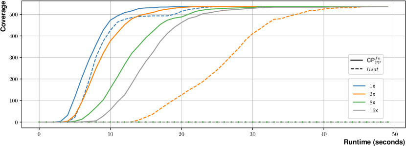
Figure 2: Ablation study on the runtime performance of $lisat$ and CP${}^{fn}_{\text{PP}}$ by scaling up the duration of the jobs in MMPSP by a factor of $2$, $8$ and $16$, respectively.

Performance over benchmarks We now discuss the observed performance (see Table 2) measured as coverage or number of instances solved optimally (or sub-optimally) per problem domain in each benchmark. Also, we look closely at the sensitivity of $lisat$ and CP${}_{\text{PP}}^{fn}$ to increasing duration of jobs in Figure 2.

The CP Planners perform very well on all formulations of the HTG instances of blocksworld domain. Table 2 reveals that every configuration of the CP planner solves the full set of HTG instances. Comparing the results on blocksworld across to the IPC instance set3, we see the CP${}_{\text{PP}}^{\textit{fn}}$ planner performs strongly too, even when the IPC instances require much higher number of plan steps than the HTG ones.

The CP planners and baseline lisat planners find feasible plans for many HTG childsnack instances, significantly more than the state-of-the-art $\mathrm{PL}$ baselines, but have trouble finding optimal plans. For any given childsnack instance, there is a huge number of possible optimal plans that are permutations of each other. Without specific guidance, our planners struggle with symmetries to obtain proofs of optimality quickly. Another structural feature of optimal plans which is revealed to be problematic is the plan-length. Domains where plans require many actions (HTG $ged$) are very challenging for our planners, with $lisat$ performing better and the $\mathrm{PL}$ baseline having remarkably good performance in all of these instances, and Madagascar too when its techniques to bundle several actions apply.

In rovers, the concise encoding of dependency of preconditions on static relations using the table constraints (see Section 5) helps the CP${}_{\text{PP}}^{\textit{fn}}$ achieve better optimizing performance than the baselines. The initial states of HTG rovers instances may have $10,000$s of atoms to specify the static relations, which otherwise would make the number of constraints (13) and (10) to blow up.

The satisficing performance of lisat with londex constraints against $\overline{\textit{lisat}}$ which does not use londex shows impressive gains in coverage by exploiting the structure of feasible plans to guide the search. The londex implementation of lisat restricts the supporter-supportee distance to $1$, initially. If UNSAT, it increases the distance limit by $1$ and solves again. It repeats the procedure until timeout or it finds a solution. This indicates a potential for improving the satisficing performance of the CP encoding by designing and integrating planning specific heuristics into the CP solvers.

Overall, all optimizing configurations of the CP planners perform much better than the baseline heuristic search planners on the HTG benchmark. The functional transformation of the PDDL tasks shows impressive performance gains, thereby highlighting the importance of a concise encoding of the planning problems. The performance of CP encoding with simple transformation of the PDDL task lags slightly behind lisat. With the functional transformation CP${}_{\text{PP}}^{\textit{fn}}$ planner catches up to $lisat$ and their coverage is about the same.

In the MMPSP instances, however, the CP approach shows its advantage over all other baseline planners. As we can see in Figure 2, while the CP${}_{\text{PP}}^{\textit{fn}}$ is slightly ahead of lisat for the original problems, scaling the durations only slowly degrades CP${}_{\text{PP}}^{\textit{fn}}$, but immediately makes a significant difference to lisat since it must encode much larger time domains, while CpSat only lazily grounds the integers encoding times. We note that all the baseline heuristic planners exceeded the memory limit on the original problem set itself.

Lastly, in the IPC instances3, the CP${}_{\text{PP}}^{\textit{fn}}$ planner performs much better than the baseline lisat. However, all CP planners as well as lisat do not perform as well as the baseline heuristic search planners. With an exception of blocks-3ops and organic-synthesis, the coverage of the CP planners is lower than that of heuristic search planners. This is an artifact of heuristic search being the dominant approach to planning [16]. Heuristic search planners work well with features showcased in the IPC instances, including significantly longer plans. On the other hand, their performance suffers in problem domains with large numeric types, specially over Resource-constrained planning(RCP) problems [33].

8 Related Work

While causal encodings are the road less travelled in planning as satisfiability, there is significant related work worth mentioning. Formulations based on the event calculus [46] exist yet are rarely acknowledged. We note that the event calculus $Initiates$ predicate corresponds to our notion of output pins, $Holds$ corresponds to our notion of input pin, and $Terminates$ is very much equivalent to our $\mathrm{persistence}$ predicate in Eq. (9). Constraint Programming was a natural target for research seeking more compact encodings very early [52], yet our most direct inspiration was the Cpt planning system [53], which in some of its later versions used a notion of propagator for its causal link constraints, very close to that later formalized by Ohrimenko et al. Previous work have proposed grounded encodings that used KMS notion of operator splitting [9, 44], which are structurally similar to our constraints for representing ground actions. Our formulation is entirely lifted, and the only ground atoms we are forced to use are those present in initial and goal state formulas. We end acknowledging that the power of $\mathrm{element}(\cdot)$ constraints and their applications to automated planning were revealed to us after the careful study of Francis et al. [14] and Francès and Geffner [13].

9 Discussion

This paper demonstrates that KMS notion of lifted causal encodings are an approach to planning as satisfiability that has become viable thanks to the notable advances in CP over the last decade. We have clearly barely scratched the surface of what is possible, as more propagator procedures follow directly from the formulation in this paper, seeking powerful synergistic relations between “planning-specific” ones and general propagation algorithms. The clear limit to this approach lies in the number of variables that need to be created. We also have not really looked into the possibility of integrating or reformulating existing work that is known to enhance notably the scalability of planning as satisfiability [42].

Alternatively, and perhaps ultimately too, we need to consider PDR-like formulations [50, 8], where we only need to construct a CP model covering two plan steps. We observe that Suda’s expedient of reimplementing the obligation propagation mechanism as a “Graphplan-like” algorithm strongly suggests that a CP formulation with suitably defined propagators could be very performant across PPIs with very diverse structure. Also, PDR formulations seem to be key for certifying unsolvability [8].

Appendix A $h^{m}$ heuristic over first-order logic existential formulae

In this section, we present an account of $h^{m}$ admissible heuristic [17] and its extension to the first-order logic existential formulas which we then use to test the reachability of a first-order logic formula. The heuristic function $h^{m}$ is an admissible approximation of the optimal heuristic function $h^{*}:{\cal{A}}\mapsto\mathbb{N}$, defined over a conjunction of positive and negative ground atoms ${\cal{A}}:={{\cal P}\times t_{1}\times\ldots\times t_{K_{\cal P}}\times\{\top,\bot\}}$. $h^{*}$ is defined using the regression model of the planning problem, in which we regress backwards from a goal formula using a regression function $rg_{a}:{\cal A}\mapsto{\cal A}$ with respect to a ground action $a\in{Act\times U^{K_{\alpha}}}$ [39]. We extend the regression function $rg_{a}$ to the first-order logic existential formulas and use it to define $h^{m}$ for the first-order logic formulas.

Let $\psi$ be a first-order logic existential formula, $\psi:=\exists\bar{x},\psi^{L}\land\psi^{EQ}$, where $\bar{x}:=(x_{1},x_{2},\ldots,x_{n})$ is a vector of parameters, $\psi^{L}$ is a conjunction of literals whose interpretation is set by the states $s\in S^{R}_{P}$, and $\psi^{EQ}$ is an equality-logic formula. We denote the set of literals in a formula $\phi$ by $\emph{lits}_{\phi}$, the predicate and the argument variables of a literal $l\in\emph{lits}_{\phi}$ by $\emph{predicate}_{l}$ and $\overline{arg}_{l}$, respectively, and the polarity of $l$ by $\emph{polarity}_{l}$.

The regression of the formula $\psi$ with respect to an action schema $\alpha:=\left<{\rm Phys.\leavevmode\nobreak\ Rev.\leavevmode\nobreak\ E}{\alpha},\mathrm{Eff}_{\alpha}\right>$ involves identifying the supporter-supportee pairs and the inconsistent literal pairs between $\mathrm{Eff}_{\alpha}$ and $\psi^{L}$. A supporter-supportee relationship holds between $l\in\emph{lits}_{\mathrm{Eff}_{\alpha}}$ and $l^{\prime}\in\emph{lits}_{\psi^{L}}$ iff the predicate and the arguments of $l$ match that of $l^{\prime}$ and they have the same polarity. On the other hand, a literal $l\in\emph{lits}_{\mathrm{Eff}_{\alpha}}$ is inconsistent with $l^{\prime}\in\emph{lits}_{\psi^{L}}$ iff the predicate and the arguments of $l$ match that of $l^{\prime}$ but they have the opposite polarity.

While regressing with respect to action schema $\alpha$, we need to consider every possible combination of supporter-supportee pairs, i.e. all subsets of the set of potential supporter-supportee pairs $\emph{SP}:=\{(l,l^{\prime})\mid\emph{polarity}_{l}=\emph{polarity}_{l^{\prime}},\leavevmode\nobreak\ \emph{predicate}_{l}=\emph{predicate}_{l^{\prime}},\ l\in\emph{lits}_{\mathrm{Eff}_{\alpha}},l^{\prime}\in\emph{lits}_{\psi^{L}}\}$, then for each literal pair $(l,l^{\prime})$ in the subset we add the constraint $\bigwedge_{i=1}^{K_{\cal P}}{arg}_{li}={arg}_{l^{\prime}i}$ to the formula obtained through regression. Thus, the regression of $\psi$ with respect to $\alpha$ produces a set of formulas, one for each subset in SP. Similarly, for each pair in the set of potential inconsistent pairs $\textit{IP}:=\{(l,l^{\prime})\mid\emph{polarity}_{l}\neq\emph{polarity}_{l^{\prime}},\leavevmode\nobreak\ \emph{predicate}_{l}=\emph{predicate}_{l^{\prime}},\ l\in\emph{lits}_{\mathrm{Eff}_{\alpha}},l^{\prime}\in\emph{lits}_{\psi^{L}}\}$, we add the constraint $\bigvee_{i=1}^{K_{\cal P}}{arg}_{li}\neq{arg}_{l^{\prime}i}$ to the regression formula of $\psi$. We now present the definition of the regression function over first-order logic formulas.

$$rg_{\alpha}(\psi):=\{\exists\bar{x},\ \widehat{rg}_{\alpha}(\psi^{L},\widetilde{\emph{SP}})\land\widecheck{rg}_{\alpha}(\psi^{EQ},\widetilde{\emph{SP}})\mid\widetilde{\emph{SP}}\subseteq\emph{SP}\}$$ (21a)

$$\widehat{rg}_{\alpha}(\psi^{L},\widetilde{\emph{SP}}):=\text{Pre}_{\alpha}\land\bigwedge_{l\in\{\emph{lits}_{\psi^{L}}\backslash\{l^{\prime}\mid(l,l^{\prime})\in\widetilde{\emph{SP}}\}\}}l$$ (21b)

$$\widecheck{rg}_{\alpha}(\psi^{EQ},\widetilde{\emph{SP}}):=\psi^{\prime EQ}\land\bigwedge_{(l,l^{\prime})\in\widetilde{\emph{SP}}}\land_{i=1}^{K_{\cal P}}arg_{li}=arg_{l^{\prime}i}\land\bigwedge_{(l,l^{\prime})\in\textit{IP}}\lor_{i=1}^{K_{\cal P}}arg_{li}\neq arg_{l^{\prime}i}$$ (21c)

where we obtain the regression of $\psi^{L}$ by removing the supportees in the set $\widetilde{\emph{SP}}$ from $\psi^{L}$ and adding the precondition of $\alpha$. The regression of $\psi^{EQ}$ involves a reduction into a canonical form $\psi^{\prime EQ}$ by setting the equality atoms whose arguments do not appear in the arguments of the regression $\widehat{rg}_{\alpha}(\psi^{L},\widetilde{\emph{SP}})$ to true. Then, we add two equality logic formulas, first of which binds the arguments of supporter-supportee pairs in $\widetilde{\emph{SP}}$ and the second disallows inconsistent assignments to the arguments of literals pairs in IP.

The $h^{m}$ heuristics for $\psi:=\exists\bar{x},\psi^{L}\land\psi^{EQ}$ is defined using regression as follows

$$h^{m}(\psi):=\begin{cases}0,&s_{0}\models\psi\\ min_{\psi^{\prime}\in rg_{\alpha}(\psi),\alpha\in\textit{Act}}h^{m}(\psi^{\prime})+cost(\alpha),&|\textit{lits}(\psi^{L})|\leq m\\ max_{\psi\vdash\psi^{\prime},|\textit{lits}(\psi^{\prime\textit{L}})|\leq m}h^{m}(\psi^{\prime}),&\textit{otherwise}\end{cases}$$ (22)

$h^{m}(\psi_{\mathsf{P}})$ can be efficiently computed using dynamic programming with memoization, and $s_{0}\models\psi$ can be encoded as a CP program with equality and table constraints. For a fixed value of $m$, the complexity of the above procedure is low polynomial in the number of nodes, i.e. the number of first-order logic formulas $O({|{\cal P}|^{m}}\cdot 2^{K_{\cal P}})$. An important property of the above procedure is that it is entirely lifted, i.e. no ground atom would occur in the formulas obtained through regression if no action schema has ground atoms. This is specially useful in hard-to-ground(HTG) domains where the size of ground theory renders the translation methods [21] used by most planners intractable.

Appendix B Proofs

Theorem B.1 (Systematicity [31]).

Let $T_{P,N_{\pi}}$ $=$ $({\cal X}$, ${\cal C})$ be the CSP given by the decision variables ${\cal X}$ in Table 1 and set of constraints ${\cal C}$ $(4)$–$(12)$, for some suitable choice of $N_{\pi}$. There exists an assignment $\xi$ onto variables ${\cal X}$ that satisfies every constraint in ${\cal C}$ if an only if there exists a feasible solution $\sigma$ to the PPI $P$, whose actions are given by slots, argument, input and output pin variables values.

Proof B.2.

It follows trivially from the definitions given in the previous sections that assignments $\xi$ encode finite trajectories $\sigma=s_{0}a_{1}s_{1}\ldots s_{N_{\pi}}$. To prove the forward direction, it suffices to observe that (1) constraints $(5)$ on input and output pins for a slot $i$ define implicitly sets of pairs of states $(s_{i-1},s_{i})\in\to_{act_{i}}$, the set of transitions corresponding to the schema $act_{i}=\alpha$ assigned to the slot, (2) constraints $(11)$ ensure that for $i=1$ the predecessor of $s_{1}$ corresponds with the initial state $s_{0}$ given in the definition of the PPI $P$, and (3) the last state in the trajectory given by $\xi$ the equality atoms in $Goal$. To prove the reverse direction, we note that each pair of consecutive states $s_{i-1}$ and $s_{i}$ must belong to exactly one of the transition sets $\to_{\alpha}$. From the definition of this set the schema, argument and pins assignments follow directly.$\square$

Theorem B.3.

If ${\cal R}_{P}$ is a mapping in all possible interpretations $s\in S^{R}_{\Pi}$, then ${\Pi^{\prime}}$, the transformation of the problem ${\Pi}$ which encodes the predicate $P$ as a function $f_{P}:\mathrm{Dom}_{x}\mapsto\mathrm{Dom}_{y}$, has the same set of reachable states as $\Pi$, i.e. $S^{R}_{\Pi}=S^{R}_{\Pi^{\prime}}$

Proof B.4.

If the right-unique and left-total properties hold for ${\cal R}_{P}$ in all $s\in S^{R}_{\Pi}$, then applying the functional transformation would not alter the reachable state space since the functional transformation implicitly enforces the same conditions, i.e. $\forall\ x_{1},x_{2}\in\mathrm{Dom}_{x},y_{1},y_{2}\in\mathrm{Dom}_{y},\ (f_{P}(x_{1})=y_{1})\land(f_{P}(x_{2})=y_{2})\land(x_{1}=x_{2})\rightarrow(y_{1}=y_{2})$ and $\forall\ x\in\mathrm{Dom}_{x},\ \exists\ y\in\mathrm{Dom}_{y},\ (f_{P}(x)=y)$.$\square$

Appendix C Additional Results: Figures and Tables

Figure 3 depicts the performance profiles of CP${}_{0}^{\textit{fn}}\mathrm{(1)}$, CP${}_{\text{PP}}^{\textit{fn}}\mathrm{(2)}$, cpddl$\mathrm{(3)}$ and lmcut$\mathrm{(4)}$, and Table 3 shows of coverage of baseline and CP planners on the IPC benchmarks.

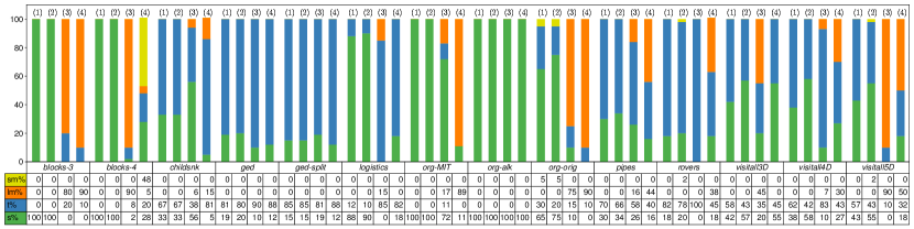
Figure 3: Plot depicting performance profiles of CP${}_{0}^{\textit{fn}}\mathrm{(1)}$, CP${}_{\text{PP}}^{\textit{fn}}\mathrm{(2)}$, cpddl$\mathrm{(3)}$, and lmcut$\mathrm{(4)}$ on the HTG benchmark set. The percentage of instances which solved $\mathrm{(s\%)}$ (optimally), reported memout during loading step $\mathrm{(lm\%)}$, reported memout during the search $\mathrm{(sm\%)}$, and timed-out $\mathrm{(t\%)}$ are shown.

IPCs(opt)	Optimal Solution
Domain	$\#$Instances	CP0	CP${}_{\text{PP}}$	CP${}_{\text{PP}}^{\textit{fn}}$	LiSAT	lmcut	sbd	cpddl	delfi1
Not-grounded - action schemas do not have ground atoms
barman-opt11	20	0	0	0	0	4	9	12	7
barman-opt14	14	0	0	0	0	0	3	6	2
blocks	35	17	19	28	26	28	30	31	27
blocks-3ops	35	19	23	35	5	26	25	30	20
childsnack-opt14	20	0	0	0	0	0	4	4	6
data-network-opt18	20	14	15	15	0*	20	17	17	17
depot	22	1	1	2	2	7	5	7	12
driverlog	20	4	4	4	5	14	12	12	15
elevators-opt08	30	2	3	5	6	20	22	23	20
elevators-opt11	20	1	1	3	4	17	18	18	16
floortile-opt11	20	0	0	0	0	6	14	14	12
floortile-opt14	20	0	0	0	0	5	20	20	17
freecell	80	6	6	6	12	15	21	22	18
ged-opt14	20	19	19	20	20	20	20	20	20
grid	5	1	1	2	1	2	2	2	3
gripper	20	1	2	2	2	7	20	20	20
hiking-opt14	20	4	4	4	8	9	14	15	19
logistics00	28	2	2	3	6	20	18	19	21
logistics98	35	0	0	1	1	6	5	5	8
miconic	150	22	23	30	32	141	104	104	136
mprime	35	31	32	33	33	22	23	25	25
mystery	30	18	18	18	19	17	13	15	17
nomystery-opt11	20	6	6	6	10	14	13	14	14
organic-synthesis-opt18	20	20	20	20	20	7	7	13	8
organic-synthesis-split-opt18	20	8	12	12	10	16	13	8	12
parking-opt11	20	1	1	1	1	2	1	1	5
parking-opt14	20	0	0	0	0	3	0	1	7
pegsol-08	30	9	8	11	20	27	28	29	28
pegsol-opt11	20	1	1	1	6	17	18	19	18
pipesworld-notankage	50	12	12	12	14	17	15	15	25
pipesworld-tankage	50	9	10	11	11	12	16	17	22
rovers	40	4	4	4	4	8	14	14	12
satellite	36	3	3	4	5	7	10	11	14
scanalyzer-08	30	10	9	13	12	9	13	13	17
scanalyzer-opt11	20	7	6	10	9	6	10	10	13
sokoban-opt08	30	0	0	0	2	24	25	28	28
sokoban-opt11	20	0	0	0	0	19	20	20	20
spider-opt18	20	0	0	0	0	6	6	6	8
storage	30	12	11	13	0*	15	14	15	17
termes-opt18	20	0	0	0	0	5	16	16	12
tetris-opt14	17	2	2	3	3	5	10	12	13
tidybot-opt11	20	1	3	3	0*	14	12	11	17
tidybot-opt14	20	0	0	0	0*	9	5	7	13
tpp	30	4	4	4	5	7	8	8	11
transport-opt08	30	6	6	6	6	12	14	14	13
transport-opt11	20	1	1	1	1	8	10	11	10
transport-opt14	20	1	1	1	2	7	9	10	9
visitall-opt11	20	8	9	11	11	10	12	12	17
visitall-opt14	20	2	3	5	5	5	6	6	13
woodworking-opt08	30	7	7	7	10	17	30	29	28
woodworking-opt11	20	2	2	2	5	12	20	20	20
zenotravel	20	7	7	8	9	13	9	0	12
Partially-grounded - action schemas have a few ground atoms
agricola-opt18	20	0	0	0	3	0	14	12	10
airport	50	6	7	7	7	28	23	24	23
movie	30	30	30	30	0*	30	30	30	30
openstacks-opt08	30	0	1	1	2	8	30	30	30
openstacks-opt11	20	0	0	0	0	3	20	20	20
openstacks-opt14	20	0	0	0	0	0	15	16	12
parcprinter-08	30	6	6	6	0*	22	30	30	30
parcprinter-opt11	20	3	3	3	0*	16	20	20	20
pathways	30	3	4	4	0*	5	5	5	5
snake-opt18	20	3	3	6	0*	7	3	5	11
Fully-grounded - action schemas only have ground atoms
openstacks	30	0	0	0	0	7	18	17	11
petri-net-alignment-opt18	20	0	0	0	0	3	18	20	20
psr-small	50	44	46	46	0*	49	50	50	50
trucks	30	2	2	2	0*	10	11	14	9
Total	1862	402	423	485	375	927	1090	1124	1195

Table 3: Coverage of different planners on IPCs – optimal track benchmark domains. * indicates the domains in which the preprocessing (parsing and encoding) step of lisat rendered the instances unsolvable.

References

- [1] Mohammad Abdulaziz, Charles Gretton, and Michael Norrish. A State-Space Acyclicity Property for Exponentially Tighter Plan Length Bounds. In Int’l Conference on Automated Planning and Scheduling (ICAPS), volume 27, pages 2–10, 2017. doi:10.1609/icaps.v27i1.13837.
- [2] José L. Balcázar. The complexity of searching implicit graphs. Artificial Intelligence, 86(1):171–188, 1996. doi:10.1016/0004-3702(96)00014-8.
- [3] A. Blum and M. L. Furst. Fast planning through planning graph analysis. In Int’l Conference on Automated Planning and Scheduling (ICAPS), 1995.
- [4] Blai Bonet and Hector Geffner. Planning as heuristic search. Artificial Intelligence, 129:5–33, 2001.
- [5] Nicholas Bourbaki. Elements of Mathematics: Theory of Sets. Springer-Verlag, 1968.
- [6] Yixin Chen, Ruoyun Huang, Zhao Xing, and Weixiong Zhang. Long-distance mutual exclusion for planning. Artificial Intelligence, 173(2):365–391, 2009.
- [7] Augusto B Corrêa, Florian Pommerening, Malte Helmert, and Guillem Frances. Lifted successor generation using query optimization techniques. In Int’l Conference on Automated Planning and Scheduling (ICAPS), 2020.
- [8] Salomé Eriksson and Malte Helmert. Certified Unsolvability for SAT Planning with Property Directed Reachability. In Int’l Conference on Automated Planning and Scheduling (ICAPS), 2020.
- [9] Michael D. Ernst, Todd D. Millstein, and Daniel S. Weld. Automatic SAT-Compilation of Planning Problems. In Proc. Int’l Joint Conference on Artificial Intelligence (IJCAI), 1997.
- [10] Daniel Fišer. cpddl: a library for automated planning. https://gitlab.com/danfis, 2022.
- [11] ABKFM Fleury and Maximilian Heisinger. Cadical, kissat, paracooba, plingeling and treengeling entering the sat competition 2020. SAT COMPETITION, 2020:50, 2020.
- [12] Guillem Francès. Effective Planning with Expressive Languages. PhD thesis, DTIC, 2017.
- [13] Guillem Frances and Hector Geffner. Modeling and computatio in planning: Better heuristics from more expressive languages. In Int’l Conference on Automated Planning and Scheduling (ICAPS), 2015.
- [14] Kathryn Francis, Jorge Navas, and Peter J. Stuckey. Modelling Destructive Assignments. In Int’l Conference on Principles and Practice of Constraint Programming (CP), pages 315–330, 2013. doi:10.1007/978-3-642-40627-0\_26.
- [15] Hector Geffner. Planning Graphs and Knowledge Compilation. In Proc. of Principles of Knowledge Representation and Reasoning (KR), 2004.
- [16] Hector Geffner and Blai Bonet. A concise introduction to models and methods for automated planning. Synthesis Lectures on Artificial Intelligence and Machine Learning, 8(1):1–141, 2013.
- [17] P Haslum H Geffner and Patrik Haslum. Admissible heuristics for optimal planning. In Proceedings of the 5th Internat. Conf. of AI Planning Systems (AIPS 2000), pages 140–149, 2000.
- [18] C. Green. Application of theorem proving to problem solving. In Proc. Int’l Joint Conference on Artificial Intelligence (IJCAI), 1969.
- [19] A. Haas. The case for domain-specific frame axioms. In The Frame Problem in Artificial Intelligence. Morgan Kaufmann, 1987.
- [20] Patrik Haslum, Nir Lipovetzky, Daniele Magazzeni, and Christian Muise. An introduction to the planning domain definition language. Synthesis Lectures on Artificial Intelligence and Machine Learning, 13(2):1–187, 2019.
- [21] Malte Helmert. The fast downward planning system. JAIR, 26:191–246, 2006.
- [22] Malte Helmert and Carmel Domshlak. Landmarks, critical paths and abstractions: what’s the difference anyway? In Int’l Conference on Automated Planning and Scheduling (ICAPS), 2009.
- [23] Jörg Hoffmann and Bernhard Nebel. The ff planning system: Fast plan generation through heuristic search. Journal of Artificial Intelligence Research, 14:253–302, 2001.
- [24] John N Hooker et al. Integrated methods for optimization, volume 170. Springer, 2012.
- [25] Daniel Höller and Gregor Behnke. Encoding lifted classical planning in propositional logic. In Proceedings of the International Conference on Automated Planning and Scheduling, volume 32, page 134–144, 2022.
- [26] International planning competitions – classical tracks. https://www.icaps-conference.org/competitions/, 1998-2018. Accessed: 19-10-2022.
- [27] Michael Katz, Shirin Sohrabi, Horst Samulowitz, and Silvan Sievers. Delfi: Online planner selection for cost-optimal planning. IPC-9 planner abstracts, pages 57–64, 2018.
- [28] Henry Kautz, David McAllester, and Bart Selman. Encoding Plans in Propositional Logic. In Proc. of Principles of Knowledge Representation and Reasoning (KR), 1996b.
- [29] Henry Kautz and Bart Selman. Planning as satisfiability. In Proc. of European Conference in Artificial Intelligence (ECAI), 1992.
- [30] Pascal Lauer, Alvaro Torralba, Daniel Fišer, Daniel Höller, Julia Wichlacz, and Jörg Hoffmann. Polynomial-time in pddl input size: Making the delete relaxation feasible for lifted planning. In Int’l Conference on Automated Planning and Scheduling (ICAPS), 2021.
- [31] David McAllester and David Rosenblitt. Systematic nonlinear planning. In Proc. of the AAAI Conference (AAAI), 1991.
- [32] J. McCarthy and P. J. Hayes. Some philosophical problems from the standpoint of Artificial Intelligence. Machine Intelligence, 4:463–502, 1969.
- [33] Hootan Nakhost, Jörg Hoffmann, and Martin Müller. Resource-constrained planning: A monte carlo random walk approach. In Proceedings of the International Conference on Automated Planning and Scheduling, volume 22, pages 181–189, 2012.
- [34] Robert Nieuwenhuis and Albert Oliveras. DPPL(T) with Exhaustive Theory Propagation and Its Applications to Difference Logic. In Proc. of the Int’l Conf. on Computer Aided Verification (CAV), pages 321–334, 2005. doi:10.1007/11513988\_33.
- [35] Olga Ohrimenko, Peter J. Stuckey, and Michael Codish. Propagation via lazy clause generation. Constraints, 14(3):357–391, 2009. doi:10.1007/s10601-008-9064-x.
- [36] Judea Pearl. Heuristics: Intelligent Search Strategies for Computer Problem Solving. Addison-Wellesley, 1984.
- [37] Laurent Perron and Vincent Furnon. Or-tools. https://developers.google.com/optimization/, 2022.
- [38] S. Richter and M. Westphal. The LAMA Planner: Guiding Cost-Based Anytime Planning with Landmarks. Journal of Artificial Intelligence Research, 39:127–177, 2010. doi:10.1613/jair.2972.
- [39] Jussi Rintanen. Regression for classical and nondeterministic planning. ECAI 2008, page 568–572, 2008. doi:10.3233/978-1-58603-891-5-568.
- [40] Jussi Rintanen. Planning with SAT, Admissible Heuristics and A*. In Proc. Int’l Joint Conference on Artificial Intelligence (IJCAI), 2011.
- [41] Jussi Rintanen. Planning as satisfiability: Heuristics. Artificial Intelligence, 193:45–86, 2012. doi:10.1016/j.artint.2012.08.001.
- [42] Jussi Rintanen. Madagascar: Scalable planning with sat. Proceedings of the 8th International Planning Competition (IPC-2014), 21:1–5, 2014.
- [43] J. A. Robinson. A Machine-Oriented Logic Based on the Resolution Principle. Journal of the ACM (JACM), 12(1):23–41, 1965. doi:10.1145/321250.321253.
- [44] Nathan Robinson, Charles Gretton, Duc-Nghia Pham, and Abdul Sattar. A Compact and Efficient SAT Encoding for Planning. In Int’l Conference on Automated Planning and Scheduling (ICAPS), 2008.
- [45] Jendrik Seipp, Florian Pommerening, Silvan Sievers, and Malte Helmert. Downward Lab. https://doi.org/10.5281/zenodo.790461, 2017.
- [46] Murray Shanahan and Mark Witkowski. Event Calculus Planning Through Satisfiability. Journal of Logic and Computation, 14(5):731–745, 2004. doi:10.1093/logcom/14.5.731.
- [47] A Sprecher and R Kolisch. Psplib—a project scheduling problem library. Eur. J. Oper. Res, 96:205–216, 1996.
- [48] Matthew Streeter and Stephen F. Smith. Using Decision Procedures Efficiently for Optimization. In Int’l Conference on Automated Planning and Scheduling (ICAPS), 2007.
- [49] Peter J. Stuckey, T. Feydy, A. Schutt, Guido Tack, and J. Fischer. The MiniZinc challenge 2008-2013. AI Magazine, 35(2):55–60, 2014.
- [50] M Suda. Property Directed Reachability for Automated Planning. Journal of Artificial Intelligence Research, 50:265–319, 2014. doi:10.1613/jair.4231.
- [51] Alvaro Torralba, Vidal Alcázar, Peter Kissmann, and Stefan Edelkamp. Efficient symbolic search for cost-optimal planning. Artificial Intelligence, 242:52–79, 2017. doi:10.1016/j.artint.2016.10.001.
- [52] Peter van Beek and Xinguang Chen. CPlan: A Constraint Programming Approach to Planning. In Proc. of the AAAI Conference (AAAI), 1999.
- [53] Vincent Vidal and Hector Geffner. Branching and pruning: an optimal temporal POCL planner based on constraint programming. Artificial Intelligence, 170:298–335, 2006.