Complexity, scaling, and a phase transition

Abstract

We investigate the holographic complexity of CFTs compactified on a circle with a Wilson line, dual to magnetized solitons in AdS₄ and AdS₅. These theories have a confinement-deconfinement phase transition as a function of the Wilson line, and the complexity of formation acts as an order parameter for this transition. Through explicit calculation, we show that proposed complexity functionals based on volume and action obey a scaling relation with radius of the circle and further prove that a broad family of potential complexity functionals obeys this scaling behavior. As a result, we conjecture that the scaling law applies to the complexity of conformal field theories on a circle in more general circumstances.

1 Introduction

Holographic complexity is the gravity-side dual of the (circuit) complexity of a gauge theory in the AdS/CFT correspondence, which is itself a measure of the Hilbert space distance of the gauge theory’s state from some reference state. There is by now a large literature studying holographic complexity (see arxiv:1403.5695 ; arXiv:1406.2678 ; arXiv:1509.07876 ; arXiv:1512.04993 for some foundational work and arXiv:2110.14672 for more references and a recent review); because there are continous families of distance measures and possible reference states, it is clear that there should be many formulations of holographic complexity. Indeed, arXiv:2111.02429 ; arXiv:2210.09647 demonstrated that a large family of functionals in asymptotically AdS spacetimes have the expected behavior of complexity on thermal states.

As a result, it is the change of complexity in parameter space rather than the value that is physically important; often, as in black hole spacetimes, the time derivative of complexity is the quantity of interest. It is also important to understand the variation of complexity with other parameters, even in static situations. To that end, we examine the holographic complexity of a CFT on a circle as a function of the radius and the Wilson line around the circle (of a $U(1)$ gauge field). The gravitational dual of the compactified CFT with Wilson line is a magnetized generalization of the AdS soliton first discussed by hep-th/9808079 ; hep-th/9803131 ; as in the standard AdS soliton, the periodic direction of the magnetized solitons shrinks at a finite AdS radius arXiv:1205.6998 ; arXiv:1807.07199 ; arXiv:2009.14771 ; arXiv:2104.14572 , meaning that the spacetime has no horizon. Moreover, if the Wilson line is below a critical value, the soliton has negative energy (compared to AdS spacetime), so it is the ground state with those boundary conditions, and the gauge theory exhibits confinement. At larger Wilson lines, the soliton energy becomes positive, so the system has a (zero-temperature) confinement-deconfinement phase transition — empty AdS with a periodic boundary direction and a Wilson line is the ground state.

Reynolds and Ross arXiv:1712.03732 evaluated the holographic complexity of the standard AdS soliton. Here, we extend their work by evaluating the complexity of formation of the magnetized solitons in AdS₄ and AdS₅, the difference in the complexity between the soliton and AdS with periodic boundary arXiv:1509.07876 ; arXiv:1512.04993 ; arXiv:1610.08063 . Since the ground state with large Wilson line corresponds to periodic AdS, the complexity of formation vanishes in the deconfined phase and acts as an order parameter for the phase transition. To our knowledge, this is the first investigation of complexity as an order parameter in a first-principles confining scenario in holography. As emphasized in arXiv:2104.14572 , the state with critical Wilson line is also supersymmetric, so tuning the Wilson line also allows us to examine the effect of supersymmetry breaking on complexity.

After reviewing the magnetized soliton backgrounds in section 2, we will consider the complexity of formation as calculated both as a volume (of a maximal spatial slice and of a spacetime region) in section 3 and as an action in section 4. In addition to finding the dependence of complexity on the Wilson line, we demonstrate that the density of complexity of formation (per unit volume of the boundary CFT) scales as the inverse $(d-1)$st power of the circumference of the boundary circle. This scaling behavior persists for a large family of possible formulations for holographic complexity, as we discuss in section 5. Reynolds and Ross arXiv:1712.03732 first found this scaling for the standard soliton (and a consistent decrease in complexity with increasing radius for a lattice fermion model); our major results on the scaling are that it factors from the dependence on the Wilson line and a proof that it is universal for any holographic complexity functional obeying a few assumptions.

We summarize our results and make some conjectures in section 6.

2 Magnetized AdS solitons and phase transition

Here, we review the geometry of magnetized AdS_d+1 solitons along with the corresponding physics of the dual gauge theory, largely following the results of arXiv:2104.14572 . Suppose that the gauge theory is on a flat spacetime with one spatial coordinate $\phi$ periodically identified with period $\Delta\phi$. In this case, the gauge theory can have a $U(1)$ Wilson line around the $\phi$ direction, and there are three regular solutions of the holographic dual gravity theory with a $U(1)$ gauge field. (This is a bosonic subsector of gauged supergravity with 8 supercharges in either 4 or 5 dimensions, and we limit our calculations to $d=3,4$.)

The first solution is AdS with a periodic direction and a Wilson line in the bulk. For reference, the metric and gauge field are

$$ds^{2}=\frac{r^{2}}{l^{2}}\left(-dt^{2}+d\vec{x}^{2}+d\phi^{2}\right)+\frac{l^{2}}{r^{2}}dr^{2},\quad A=-\frac{\Phi}{\Delta\phi}d\phi$$ (1)

for holonomy $\Phi$ of the boundary gauge field. The other two solutions are generalizations of the AdS soliton; both have metric (for $d=3,4$)

$$ds^{2}=\frac{r^{2}}{l^{2}}\left(-dt^{2}+d\vec{x}^{2}+f(r)d\phi^{2}\right)+\frac{l^{2}}{r^{2}f(r)}dr^{2},\quad f(r)\equiv 1-\frac{\mu l^{2}}{r^{d}}-\frac{Q^{2}l^{2}}{r^{2d-2}}$$ (2)

and gauge field

$$A=\sqrt{7-d}\,Q\left(\frac{1}{r^{d-2}}-\frac{1}{r_{0}^{d-2}}\right)d\phi,\quad Q\equiv\frac{1}{\sqrt{7-d}}\frac{r_{0}^{d-2}\Phi}{\Delta\phi}.$$ (3)

Like the AdS soliton, the bulk spacetimes terminate at $r_{0}$, the largest root of $f(r)$; for the soliton geometries to be regular at $r_{0}$, $\mu$ must yield

$$\Delta\phi=\frac{4\pi l^{2}}{r_{0}^{2}f^{\prime}(r_{0})}$$ (4)

(note that $\phi$ has units of length, so $\Delta\phi$ is a circumference). There are two solutions to $f(r_{0})=0$ and (4) for both values of $d$ we consider:

$$\mu=\frac{r_{0}^{2d-2}-Q^{2}l^{2}}{l^{2}r_{0}^{d-2}},\quad r_{0}=\frac{2\pi l^{2}}{d\Delta\phi}\left(1\pm\sqrt{1-\frac{\Phi^{2}}{\Phi_{max}^{2}}}\right)$$ (5)

with $\Phi_{max}=g(d)\pi l$, $g(d)=\sqrt{(46-10d)/d}$. The shorter soliton, ie, the solution with larger $r_{0}$, goes to the AdS soliton for $Q=0$, whereas the longer soliton merges with the periodic AdS solution in that limit. For completeness, we note that the two magnetic solitons have field strength

$$F=-\sqrt{7-d}(d-2)\frac{Q}{r^{d-1}}dr\wedge d\phi.$$ (6)

With the usual boundary conditions of fixed geometry and gauge field, the variables of the CFT are the periodicity $\Delta\phi$ and Wilson line $\Phi$.

There are two methods to determine the energy density of each solution and therefore the ground state of the CFT with given periodicity and Wilson line. Because it will be useful later, we give the holographic renormalization argument here. We make a Fefferman-Graham expansion fg of the asymptotic form of the bulk metric as

$$ds^{2}=l^{2}\frac{dz^{2}}{z^{2}}+\frac{l^{2}}{z^{2}}\left(\gamma^{(0)}_{ij}+\sum_{n=d}^{\infty}z^{n}\gamma^{(n)}_{ij}\right)dx^{i}dx^{j};$$ (7)

with $z=0$ at the boundary (and $x^{i}=[t,\vec{x},\phi]$ in our case). Generally, the sum can include terms with $1\leq n<d$ as well as terms proportional to $z^{n}\ln(z)$ for $n\geq d$ and $d$ even, although those terms vanish for the solitons we consider. Apparently

$$\int\frac{dz}{z}=-\int\frac{dr}{r\sqrt{f(r)}}\quad\Rightarrow\quad\ln(z/l)=-\ln(r/l)+\frac{\mu l^{2}}{2dr^{d}}+\cdots$$ (8)

using a large radius expansion. Solving iteratively,

$$r=\frac{l^{2}}{z}\left(1+\frac{\mu l^{2}}{2d}\frac{z^{d}}{l^{2d}}+\cdots\right).$$ (9)

In holographic renormalization (see for example hep-th/0002230 ; arxiv:1211.6347 ), the boundary stress tensor is $\langle T_{ij}\rangle=dl^{d-1}\gamma^{(d)}_{ij}/16\pi G+\cdots$, where $G$ is the $(d+1)$-dimensional Newton constant in the AdS spacetime and the dots are terms that vanish on the soliton solutions. The energy density is therefore $\langle T_{tt}\rangle=-\mu/16\pi Gl^{d-1}$. The long soliton ($r_{0}$ small) has negative $\mu$ and positive energy density always, while the short soliton has negative energy at small $\Phi$ and positive energy when $\Phi\geq\Phi_{S}\equiv 2\pi l/[\sqrt{3}]$ for $d=3$ [$d=4$]. Therefore, the system undergoes a phase transition from the short soliton at small $\Phi$ to periodic AdS for $\Phi>\Phi_{S}$. Since the ground state of the theory is either periodic AdS or the short soliton, we will henceforth always mean the short soliton when we discuss a soliton solution.

Because the soliton solutions cap off smoothly in the infrared rather than having a horizon, they exhibit confinement (like the standard $Q=0$ AdS soliton hep-th/9808079 ; hep-th/9803131 ). As a result, the phase transition from tuning the Wilson line $\Phi$ through $\Phi_{S}$ is a confining/deconfining transition. (arXiv:2104.14572 also emphasized that the short soliton is supersymmetric at $\Phi=\Phi_{S}$.)

As noted above, the usual Dirichlet boundary condition on the gauge field $\delta A_{\mu}=0$ means that the CFT is defined in terms of fixed Wilson line $\Phi$; in thermodynamics, this is the grand canonical ensemble. With an additional term in the action for the Maxwell field on the conformal boundary of AdS (or, precisely speaking, on a cutoff surface at fixed large radius $r$), the natural variable of the CFT is $Q$ hep-th/9902170 ; arXiv:2104.14572 . The boundary term in the action means that the variational problem of the gauge field has Neumann boundary conditions ($\delta F_{\mu\nu}=0$). (Multiplication of the boundary action term by an arbitrary coefficient leads to mixed, or Robin, boundary conditions.) In the Euclidean theory, adding the boundary term gives the theory in the canonical ensemble. We will return to this point later.

3 Volume complexity of formation

The simplest proposals for holographic complexity are given in terms of a volume on the gravity side of the correspondence. The initial proposal for complexity, known as CV or “complexity=volume” arxiv:1403.5695 ; arXiv:1406.2678 , for an asymptotically AdS spacetime is $C_{V}=(d-1)V/2\pi^{2}Gl$, where $V$ is the volume of a maximal volume slice anchored at a fixed time on the boundary. While we have written the normalization of the complexity with the AdS scale $l$, the choice of length scale is ambiguous. To compare the complexity of magnetized solitons with varying Wilson line, we should choose a fixed length scale, but the overall normalization is unimportant, so we choose the AdS scale for simplicity.

All the backgrounds we consider have both time translation and time reversal symmetries, so the maximal volume surface is a constant time surface (we will always choose to measure complexity at boundary time $t=0$). Because the volume diverges near the conformal boundary, we can integrate out only to a finite radius $r_{m}$. For both the magnetized solitons and periodic AdS, this volume is

$$V=V_{\vec{x}}\Delta\phi\int_{r_{0}}^{r_{m}}dr\left(\frac{r}{l}\right)^{d-2}=\frac{V_{\vec{x}}\Delta\phi}{d-1}\frac{r_{m}^{d-1}-r_{0}^{d-1}}{l^{d-2}},$$ (10)

with $r_{0}\to 0$ for periodic AdS, where $V_{\vec{x}}$ is the volume along the $\vec{x}$ directions.

To find the complexity of formation of the soliton, we should subtract the corresponding volume of periodic AdS from (10) arXiv:1610.08063 . As a result, periodic AdS has by definition vanishing complexity of formation, and any soliton appears to have negative complexity of formation. There is a subtlety to consider, however. Rather than comparing volumes using the same cut-off radius $r_{m}$, we should compare them using the same Fefferman-Graham coordinate $z$ as defined in (8). If $r^{\prime}_{m}$ is the cut off in periodic AdS and $r_{m}$ in the soliton, then (9) implies that

$$r_{m}^{d-1}=r_{m}^{\prime d-1}\left(1+\frac{\mu l^{2}(d-1)}{2dr_{m}^{\prime d}}+\cdots\right).$$ (11)

Therefore, the divergent terms in the maximal volumes cancel as $r_{m}\to\infty$, meaning the density of complexity of formation is negative: $\mathcal{C}_{V}=-r_{0}^{d-1}/2\pi^{2}Gl^{d-1}$ in terms of the soliton radius $r_{0}$. Similarly, the difference in $r_{m}$ between solitons with different values of $\Phi$ also does not contribute as we take $r_{m}\to\infty$.

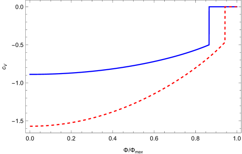
Figure 1: CV complexity of formation per unit volume for $d=3$ (solid blue) and $d=4$ (dashed red). Plotted curves are $c_{V}\equiv G\mathcal{C}_{V}(\Delta\phi/l)^{d-1}$, so complexity scales with an inverse power of $\Delta\phi$.

Two features of $\mathcal{C}_{V}$ are immediately apparent. First, it scales as an inverse power of the circumference $\mathcal{C}_{V}\propto\Delta\phi^{-(d-1)}$, and it is discontinuous at the phase transition since $r_{0}\neq 0$ at $\Phi=\Phi_{S}$. We show the dimensionless quantity $c_{V}\equiv G\mathcal{C}_{V}(\Delta\phi/l)^{d-1}$ as a function of $\Phi/\Phi_{max}$ in figure 1. Note that $c_{V}$ jumps from a negative value to zero at $\Phi=\Phi_{S}$, the supersymmetric value, because of the deconfining phase transition at that Wilson line. While the value of the complexity appears similar at $\Phi_{S}$ for the two dimensionalities, it is not equal.

The negative value of $\mathcal{C}_{V}$ is noteworthy; arXiv:2109.06883 showed that maximal volume slices in a wide variety of asymptotically AdS spacetimes are always larger than maximal slices in AdS. However, they assume maximal symmetry of the spatial slice of the conformal boundary, which the solitons (and periodic AdS) violate, so their theorems do not apply.

Another proposal for holographic complexity, known as CV2.0, is that $C_{2}\equiv V_{WDW}/Gl^{2}$, where $V_{WDW}$ is the spacetime volume of the Wheeler–DeWitt (WDW) patch arXiv:1610.02038 . The WDW patch is the spacetime region bounded by future- and past-directed lightsheets emitted from the boundary time slice where the complexity is measured; once again, we choose the length scale in the normalization as the AdS length $l$ for simplicity and note that the overall normalization of complexity is unimportant physically. In defining the WDW patch, we choose the boundary conditions that both lightsheets satisfy $t=0$ at the radial cutoff $r=r_{m}$ as a regulator, rather than taking $t=0$ as $r\to\infty$ and cutting off the patch at $r=r_{m}$. See Akhavan:2019zax ; Omidi:2020oit for a demonstration that these regulators are equivalent when properly defined in the context of action complexity.

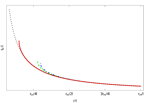
Figure 2: The future lightsheets $t_{F}(r)$ for $\Phi/\Phi_{max}=$0 (dot-dashed blue), 0.5 (dashed green), 1 (solid red). In this instance, $\Delta\phi\,r_{m}/\ell^{2}=10\pi/3$ and $d=4$. For reference, $t_{F}(r)$ for periodic AdS is dotted black.

The lightsheets on the WDW patch boundary are given by $t_{F}(r)$ and $t_{P}(r)=-t_{F}(r)$, where $F,P$ respectively designate the future and past lightsheets; they are given by $dt_{F}/dr=-l^{2}/r^{2}\sqrt{f(r)}$ and extended along $\vec{x}$ and $\phi$. For fixed $\Delta\phi\,r_{m}$, increasing $\Phi$ lengthens the soliton (decreasing $r_{0}$ for the short soliton). In addition, $t_{F}(r_{0})$ is finite but develops a cusp (infinite derivative). See figure 2 for a comparison of $t_{F}$ for several values of $\Phi/\Phi_{max}$ in $d=4$ (we choose a small value of $\Delta\phi\,r_{m}$ to emphasize the difference in the lightsheets near the soliton cap). Note that the end of each curve at the left is the end of the spacetime at $r_{0}$. For reference, we also show $t_{F}(r)=l^{2}/r-l^{2}/r_{m}$ for AdS spacetime.

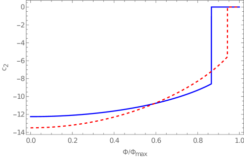
Figure 3: CV2.0 complexity of formation per boundary volume for $d=3$ (solid blue) and $d=4$ (dashed red). Plotted curves are $c_{2}\equiv G\mathcal{C}_{2}(\Delta\phi/l)^{d-1}$, so complexity scales with an inverse power of $\Delta\phi$.

Because the WDW patch volume is

$$V_{WDW}=\int_{WDW}d^{d+1}x\sqrt{-g}=2V_{\vec{x}}\Delta\phi\int_{r_{0}}^{r_{m}}dr\,\left(\frac{r}{l}\right)^{d-1}t_{F}(r),$$ (12)

we expect the complexity of formation to be negative — the increase in $t_{F}$ near $r_{0}$ is not enough to compensate for the shortening of spacetime. In appendix B, we describe the numerical calculation of $\mathcal{C}_{2}$, the density of complexity of formation, holding the Wilson line $\Phi$ (rather than $Q$) fixed. Direct calculation shows that $\mathcal{C}_{2}\propto\Delta\phi^{-(d-1)}$ as we remove the cutoff $r_{m}\to\infty$, which is notably the same scaling as $\mathcal{C}_{V}$. We therefore show $c_{2}\equiv G\mathcal{C}_{2}(\Delta\phi/l)^{d-1}$ in figure 3. Like the CV complexity of formation, the magnitude of $c_{2}$ decreases as $\Phi$ increases and jumps to zero at the deconfining phase transition.

4 Action complexity of formation

The action complexity (“complexity=action” or CA) is given by $C_{A}=S_{WDW}/\pi$, where $S_{WDW}$ is the action evaluated on the WDW patch, including appropriate terms on the boundary of the patch arXiv:1509.07876 ; arXiv:1512.04993 ; arXiv:1609.00207 . Altogether, this action is $S_{WDW}=S_{bulk}+S_{bdy}+S_{joint}$, where

$$S_{bulk} = \frac{1}{16\pi G}\int_{WDW}d^{d+1}x\sqrt{-g}\left(R+\frac{d(d-1)}{l^{2}}-\frac{1}{4}F_{\mu\nu}F^{\mu\nu}\right),$$ (13)

$$S_{bdy} = -\frac{1}{8\pi G}\int_{F}d\lambda\,d^{d-2}\vec{x}\,d\phi\sqrt{\gamma}\left(\kappa_{F}+\Theta_{F}\ln|\beta l\Theta_{F}|\vphantom{\frac{1}{2}}\right)$$ (14)

$$+\frac{1}{8\pi G}\int_{P}d\lambda\,d^{d-2}\vec{x}\,d\phi\sqrt{\gamma}\left(\kappa_{P}+\Theta_{P}\ln|\beta l\Theta_{P}|\vphantom{\frac{1}{2}}\right),$$

$$S_{joint} = -\frac{1}{8\pi G}\int_{F\cap P}d^{d-2}\vec{x}\,d\phi\sqrt{\gamma}\ln\left|k_{F}\cdot k_{P}/2\right|.$$ (15)

The action diverges, so we regulate by integrating for $r\leq r_{m}$ only and subtract the corresponding action of periodic AdS to cut-off radius $r^{\prime}_{m}$ related to $r_{m}$ by (11); note that the Wilson line does not contribute to the periodic AdS action because the field strength vanishes. The somewhat novel boundary and joint terms are by now thoroughly discussed in the literature, so we relegate a detailed description to appendix C. We note that $\beta$ is an arbitrary parameter that in principle could affect the complexity; however, it cancels in the complexity of formation when subtracting the periodic AdS action in the $r_{m}\to\infty$ limit. (In $d=4$, there is also a Chern-Simons term for the gauge field in the bulk action, but it vanishes for the soliton solutions.)

Like the boundary terms (14) for gravitational degrees of freedom, the WDW patch action includes a boundary term for the Maxwell field

$$\Delta S_{bdy}=\frac{\nu}{16\pi G}\int_{F}d\lambda\,d^{d-2}\vec{x}\,d\phi\sqrt{\gamma}k_{F}^{\mu}A^{\nu}F_{\mu\nu}+\frac{\nu}{16\pi G}\int_{P}d\lambda\,d^{d-2}\vec{x}\,d\phi\sqrt{\gamma}k_{F}^{\mu}A^{\nu}F_{\mu\nu}$$ (16)

with $\nu$ an arbitrary constant arXiv:1901.00014 . This is the lightlike analog of the term on the AdS conformal boundary that changes the natural variable of the CFT. However, as especially emphasized by the “complexity$=$anything” program arXiv:2111.02429 ; arXiv:2210.09647 , there is no logical connection between $\nu$ and the boundary conditions at $r=r_{m}$. In other words, $\nu$ can take any value regardless of whether $\Phi$ or $Q$ is the natural variable of the CFT. Also, since the complexity is given by the action evaluated on shell, $\Delta S_{bdy}$ is equivalent to a multiple of the bulk Maxwell action (in the absence of sources) arXiv:1901.00014 . As a result, we can take the prefactor of $F_{\mu\nu}F^{\mu\nu}$ to $(2\nu-1)/4$ rather than $-1/4$ in (13) rather than adding an additional boundary term.

The Wilson line in the CFT has several effects on the action complexity (evaluated at fixed periodicity $\Delta\phi$). As noted previously, increasing $\Phi$ lengthens the soliton (decreasing $r_{0}$), tending to increase the magnitudes of $S_{bulk}$ and $S_{bdy}$. The change in the shape of $t_{F}(r)$ additionally affects the expansion $\Theta_{F,P}$ of the lightsheets at the WDW patch boundary, primarily in the interior region. The field strength itself gives contributes to the Lagrangian density (including a positive semidefinite contribution to the curvature for $d\geq 3$); this contribution is negative for small $\nu$ but positive for $\nu>1/(d-1)$.

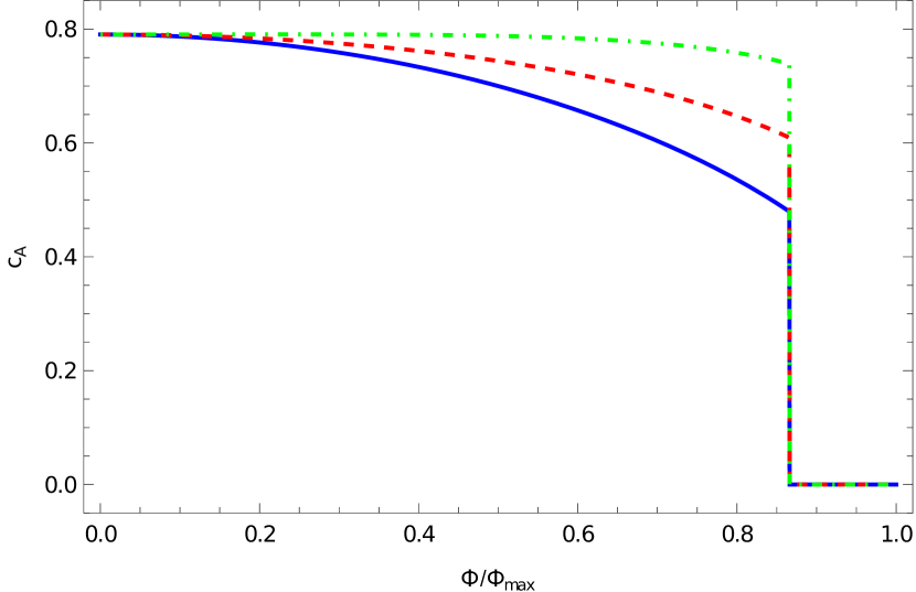
(a) $d=3$

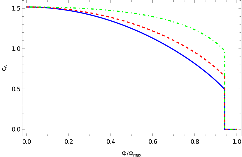
(b) $d=4$

Figure 4: CA complexity of formation per unit boundary volume for $d=3,4$ as labeled with $\nu=0$ (solid blue), $\nu=1/(d-1)$ (dashed red), and $\nu=1$ (dot-dashed green). Plotted curves are $c_{A}=G\mathcal{C}_{A}(\Delta\phi/l)^{d-1}$ as a function of the Wilson line $\Phi$.

Using the grand canonical ensemble variables $\Delta\phi,\Phi$ appropriate to standard boundary conditions on AdS, the density of complexity of formation $\mathcal{C}_{A}$ scales as $\Delta\phi^{-(d-1)}$, like the volume complexities $\mathcal{C}_{V},\mathcal{C}_{2}$, as we show in appendix C. Given that $\mathcal{C}_{A}$ is considerably more intricate to calculate than either volume complexity, it may be surprising that it obeys the same simple scaling relation. Note that this scaling does not hold in the canonical ensemble in which the complexity is evaluated as a function of $Q$. In that case, the scaling property of the action implies that $\mathcal{C}_{A}\propto\Delta\phi^{-(d-1)}$ along lines of constant $Q\Delta\phi^{d-1}$ (see equations (3,5)).

We show $c_{A}\equiv G\mathcal{C}_{A}(\Delta\phi/l)^{d-1}$ as a function of $\Phi$ in figure 4. In contrast to $\mathcal{C}_{V}$ and $\mathcal{C}_{2}$, $\mathcal{C}_{A}$ is positive semi-definite (equal zero in the deconfined phase). In the absence of the lightsheet boundary term for the Maxwell field ($\nu=0$), the complexity is maximized with no Wilson line and decreases toward $\Phi=\Phi_{S}$ (solid blue curve). For $\nu=1/(d-1)$, the $F_{\mu\nu}F^{\mu\nu}$ term cancels, so the corresponding (dashed red) curve shows only the geometric effect of the Wilson line (increased soliton length, altered WDW patch shape) on the complexity. Finally, for $\nu=1$ (dot-dashed green curve), the $d=3$ $\mathcal{C}_{A}$ curve increases at $\Phi=0$ and reaches a maximum for $\Phi<\Phi_{S}$. In this case, the (positive) contribution of the $F_{\mu\nu}F^{\mu\nu}$ term increases with $\Phi$, but the overall scaling with $r_{0}^{d-1}$ which decreases with $\Phi$ eventually dominates. For $d=4$ and $\nu=1$, $c_{A}$ decreases with increasing $\Phi$.

5 Scaling with circumference in general complexity

In the previous two sections, we have seen that the complexity of formation density $\mathcal{C}$ for magnetized AdS solitons scales as $1/\Delta\phi^{d-1}$ when $\mathcal{C}$ is written as a function of the grand canonical variables $\Delta\phi,\Phi$ and the UV cutoff goes to infinity for the CV, CV2.0, and CA holographic complexity proposals. The details of these complexity measures and some of their properties (such as positivity or negativity on the soliton) are sufficiently different that it is reasonable to suspect a general principle rather than a coincidence at work.

Specifically, arXiv:2210.09647 argued that a large family of functionals of the form

$$C=\frac{1}{Gl^{2}}\int_{\mathcal{M}}d^{d+1}x\sqrt{-g}\,\mathcal{G}+\frac{1}{Gl}\int_{\mathcal{M}^{+}}d^{d}\sigma\sqrt{h}\,\mathcal{F}^{+}+\frac{1}{Gl}\int_{\mathcal{M}^{-}}d^{d}\sigma\sqrt{h}\,\mathcal{F}^{-}$$ (17)

all satisfy basic properties expected of holographic complexity. Here $\mathcal{M}$ is a bulk region in asymptotically AdS spacetime with $\mathcal{M}^{\pm}$ respectively spacelike surfaces at the future and past portions of the boundary of $\mathcal{M}$ ($\sigma$ are worldvolume coordinates on $\mathcal{M}^{\pm}$) and $\mathcal{G},\mathcal{F}^{\pm}$ are dimensionless scalar functions of the metric (and curvatures). Since the magnetized solitons contain matter, we generalize to allow $\mathcal{G},\mathcal{F}^{\pm}$ to be functions of the gauge potential and field strength as well. $\mathcal{M}$ itself optimizes a possibly different functional of the same form. The boundaries of $\mathcal{M}^{\pm}$ form a joint at the time slice on the AdS boundary (more precisely, at the cutoff radius) where the CFT complexity is to be evaluated; arXiv:2210.09647 implies that additional contributions to $C$ on this joint are included, possibly in a manner that cancels boundary terms from the $\mathcal{M}^{\pm}$ integrals (see appendix C for example). Further, there are limits of the optimization procedure choosing $\mathcal{M}$ that leads to lightlike $\mathcal{M}^{\pm}$, so the WDW patch is a possible region $\mathcal{M}$.

We will argue here that a general complexity functional as in (17) leads to a density for complexity of formation $\mathcal{C}\propto r_{0}^{d-1}\propto\Delta\phi^{-(d-1)}$ for the magnetized soliton backgrounds described in section 2, when the soliton is considered a function of the grand canonical variables $\Delta\phi,\Phi$.

To make this argument, we assume that the complexity of empty periodic AdS is $C=(aV_{\vec{x}}\Delta\phi/G)(r_{m}/l)^{d-1}$ when evaluated with a cutoff radius $r_{m}$, where $a$ is a numerical constant. This is the behavior seen in the CV, CV2.0, and CA proposals and is the strongest divergence possible for the bulk term in AdS since curvature invariants are constant and the embedding $t_{\pm}(r)$ of $\mathcal{M}^{\pm}$ satisfies $|\partial_{r}t_{\pm}(r)|\leq l^{2}/r^{2}$ for spacelike and lightlike surfaces. The lack of subleading divergences (or a leading divergence of a lower power) means that we can write this term as

$$C=\frac{aV_{\vec{x}}\Delta\phi}{G}\left[\left(\frac{r_{0}}{l}\right)^{d-1}+(d-1)\int_{r_{0}}^{r_{m}}dr\,r^{d-2}\right],$$ (18)

which is suitable for subtraction from the soliton’s complexity.

To proceed, we rewrite the metric (2) and gauge field (3,6) in terms of rescaled coordinates $\tilde{r}=r/r_{0}$ and $\tilde{t}=r_{0}t/l$, which arXiv:1712.03732 introduced:

$$ds^{2} = \tilde{r}^{2}\left(-d\tilde{t}^{2}+\frac{r_{0}^{2}}{l^{2}}d\vec{x}^{2}+\frac{r_{0}^{2}}{l^{2}}f(\tilde{r})d\phi^{2}\right)+\frac{l^{2}}{\tilde{r}^{2}f(\tilde{r})}d\tilde{r}^{2},\quad f(\tilde{r})=1-\frac{1-\tilde{Q}^{2}}{\tilde{r}^{d}}-\frac{\tilde{Q}^{2}}{\tilde{r}^{2d-2}},$$

$$A = \sqrt{7-d}\,r_{0}\tilde{Q}\left(\frac{1}{\tilde{r}^{d-2}}-1\right)d\phi,\quad F=-\sqrt{7-d}(d-2)\,\frac{r_{0}\tilde{Q}}{\tilde{r}^{d-1}}d\tilde{r}\wedge d\phi,$$

$$\tilde{Q}^{2} \equiv \frac{d^{2}/4}{7-d}g(d)^{2}\left(\frac{\Phi}{\Phi_{max}}\right)^{2}\left(1+\sqrt{1-\Phi^{2}/\Phi_{max}^{2}}\right)^{-2}.$$ (19)

Because we are comparing the density of complexity of formation (ie, complexity per volume $V_{\vec{x}}\Delta\phi$) across different values of $\Delta\phi$ and $\Phi$, we cannot rescale the $\vec{x}$ and $\phi$ coordinates. Likewise, the UV cutoff is at a fixed value of the un-rescaled radial coordinate $r=r_{m}$ corresponding to fixed Fefferman-Graham coordinate.

In these coordinates, the tensor components $g_{\mu\nu},A_{\mu},F_{\mu\nu}$ contain precisely one factor of $r_{0}$ for each leg along $\vec{x}$ or $\phi$. It is straightforward to check that the same is true of the Riemann tensor with all indices lowered. The Christoffel symbols are also such that covariant derivatives in the $\vec{x},\phi$ directions add a factor of $r_{0}$ but those in the $\tilde{t},\tilde{r}$ directions do not (this argument also relies on translation invariance in the $\vec{x},\phi$ directions). As a result, any bulk scalar function $\mathcal{G}$ constructed from the metric, the Riemann tensor, the gauge field, or their covariant derivatives is independent of $r_{0}$ — the inverse metric components needed for contractions cancels them. In addition, on either spatial surface $\mathcal{M}^{\pm}$, the normal vector $n_{\mu}$ can have components only in the $\tilde{t},\tilde{r}$ directions due to translational invariance, and its only nonzero convariant derivatives have only those legs also. As a result, the extrinsic curvature has no factors of $r_{0}$. Similar arguments apply to the curvature $\kappa$ and expansion $\Theta$ if $\mathcal{M}^{\pm}$ is lightlike. Therefore, assuming $\mathcal{F}^{\pm}$ are constructed only from the metric, gauge field, and those curvatures, they contain no explicit factors of $r_{0}$ either. Altogether, any functional $C$ of the form (17) is proportional to $r_{0}^{d-1}$, with all those factors arising from determinants of the metric, except for a dependence on the region of integration.

Under these assumptions, the density of complexity of formation takes the form

$$\mathcal{C}=\frac{1}{G}\left(\frac{r_{0}}{l}\right)^{d-1}\left\{-a+\int_{1}^{r_{m}/r_{0}}d\tilde{r}\left[\left(\tilde{t}_{+}(\tilde{r})-\tilde{t}_{-}(\tilde{r})\right)\mathfrak{g}(\tilde{r})+\mathfrak{f}^{+}(\tilde{r};\tilde{t}_{+}(\tilde{r}))+\mathfrak{f}^{-}(\tilde{r};\tilde{t}_{-}(\tilde{r}))\right]\right\},$$ (20)

where $\mathfrak{g},\mathfrak{f}^{\pm}$ are the result of evaluating $\mathcal{G},\mathcal{F}^{\pm}$ on the soliton (with the AdS complexity subtracted), and $\tilde{t}_{\pm}(\tilde{r})$ are describe the surfaces $\mathcal{M}^{\pm}$. The dependence of $\mathfrak{f}^{\pm}$ on $\tilde{t}_{\pm}(\tilde{r})$ includes dependence on the derivatives of that embedding function. Here we give the case that $\mathcal{M}^{\pm}$ are spacelike, but the timelike case is similar (see appendix C for the example of CA complexity). From the above discussion, $\mathfrak{g},\mathfrak{f}^{\pm}$ must be independent of $r_{0}$, so the only possible dependence on $\Delta\phi$ is through the upper limit of integration or implicitly in $\tilde{t}_{\pm}$. However, $\tilde{t}_{\pm}$ are given by optimization of a functional of the form (17), in which dependence on $r_{0}$ scales out of the integrand. Therefore, $\tilde{t}_{\pm}$ depends on $r_{0}$ only through the boundary condition $\tilde{t}_{\pm}(\tilde{r}=r_{m}/r_{0})=0$. However, $\mathcal{C}$ is by design convergent in the $r_{m}\to\infty$ limit, so the integral cannot depend on $r_{0}$ in that limit. The overall scaling is therefore $\mathcal{C}\propto r_{0}^{d-1}\propto\Delta\phi^{-(d-1)}$.

6 Discussion and conjecture

To summarize, we have evaluated several proposals for holographic complexity for a 3- or 4-dimensional CFT on a circle (times Minkowski spacetime) and a $U(1)$ gauge field, which corresponds to magnetized AdS soliton backgrounds through gauge/gravity duality. One immediate observation is that “complexity=volume” proposals (both CV and CV2.0) have negative complexity of formation, while the complexity of formation for the “complexity=action” proposal is positive. As a result, we speculate that the reference states for the CV and CV2.0 proposals lie in a different region of the CFT’s Hilbert space than the reference states for CA complexity proposals (which may vary with varying boundary conditions for the gauge field). Another interpretation is that the volume and action complexity proposals have similar reference states but very different distance measures, though that seems less likely to lead to the observed sign change.

As emphasized by arXiv:2104.14572 , the compactified CFT exhibits two behaviors near the critical Wilson line value $\Phi=\Phi_{S}$: supersymmetry breaking for $\Phi\neq\Phi_{S}$ and a transition from the magnetized soliton (confining) phase to the periodic AdS (deconfined) phase. The latter effect seems to be more important for the complexity; the complexity of formation acts like an order parameter, vanishing in the deconfined phase and changing discontinously at the transition. This is perhaps unsurprising given the nature of the phase transition with periodic AdS as the ground state in the deconfined phase. On the other hand, the degree of supersymmetry breaking does not seem to influence the complexity; $\mathcal{C}$ is constant for $\Phi>\Phi_{S}$ (by definition) but $|\mathcal{C}|$ grows generically as $\Phi$ decreases below $\Phi_{S}$. (With further decreases in $\Phi$, $|\mathcal{C}|$ decreases again in some cases.)

A striking result is that the dependence of the complexity of formation on the grand canonical variables $\Delta\phi,\Phi$ factorizes, with the density behaving as $\mathcal{C}=h(\Phi)/\Delta\phi^{d-1}$, extending the original observation of arXiv:1712.03732 for the soliton without magnetic field to magnetized solitons (in $d=3,4$ only, however). This scaling law holds for the three specific forms of holographic complexity that we calculated; we further showed that the general holographic complexity functional as advocated by the “complexity=anything” program arXiv:2111.02429 ; arXiv:2210.09647 has the same scaling, under some mild assumptions. Therefore, we make a series of progressively stronger conjectures; the first is simply that this scaling extends to all magnetic AdS solitons of any dimensionality $d$. Next, we conjecture that the density of complexity of formation for any $d$-dimensional holographic field theory on a circle scales as the inverse $(d-1)$st power of the circumference, when the theory is written in terms of grand canonical variables. A stronger conjecture is that this scaling is true for the complexity of formation for any conformal field theory on a circle (or possibly even any quantum field theory).

A critical point in our arguments is the finiteness of the complexity of formation, which allows us to remove the UV cutoff (ie, take $r_{m}\to\infty$). This is manifestly true since the soliton is asymptotically AdS, so the complexity of the soliton has the same divergence structure as periodic AdS. However, for the complexity of formation to scale with the circumference as conjectured, we assumed that the complexity of AdS itself must be a pure divergence $\propto r_{m}^{d-1}$, the strongest possible divergence. If we presuppose that the density of complexity of formation should scale as $\Delta\phi^{-(d-1)}$, this gives us instead an additional requirement for a functional to describe holographic complexity (beyond the switchback effect and linear growth at late time in black hole backgrounds). Since this seems like an unnatural condition for theories with a scale, it may indicate that complexity may not have a simple scaling behavior in non-conformal theories.

Next, we note that the Casimir energy density of a $d$-dimensional field theory on one finite dimension scales as $d$ powers of the inverse length of that dimension. In fact, we can see this behavior in the holographic energy density as reviewed in section 2. It is intriguing to consider whether there is a deeper connection between the scaling of the Casimir energy and of complexity of formation. On the other hand, both scaling laws may simply arise because both are given by integration over field modes in the noncompact directions of the field theory.

Finally, it is worth considering the connection of our results to those of Andrews:2019hvq regarding the complexity of another type of soliton in AdS₅. There are two major distinctions from our work: first, the solitons considered in Andrews:2019hvq have positive energy so are never the ground state; second, they are asymptotic to AdS₅ in global coordinates, so the compact boundary dimension is instead one of the angular directions of the boundary $S^{3}$ and cannot have arbitrary circumference. As a result, it is difficult to make a direct comparison with our work. Nonetheless, Andrews:2019hvq observe that the complexity of formation for those solitons also obeys a scaling law, in their case with the thermodynamic volume of the soliton. Since AlBalushi:2020rqe observes a similar scaling for black holes, it would be interesting in the future to determine what kind of relationship there may be between that scaling law and the one we have discussed here.

Appendix A Energy density from curvature

An alternative method to determine the energy density of asymptotically AdS backgrounds is to compare the extrinsic curvature of a boundary surface at a cutoff radius $r_{m}$ to that of one with identical geometry in pure AdS, as in gr-qc/9501014 .

Specifically, we choose a surface at fixed $t$ and large $r$. The energy of the spacetime is

$$E=-\frac{1}{8\pi G}\int N(K-K_{0})$$ (21)

with the integral over the surface. Here, $N$ is the lapse, $K$ is the extrinsic curvature of the surface in the spacetime in question (the solitons in our case), and $K_{0}$ the curvature of the surface in empty AdS. The curvature is given by $K=n^{\mu}\partial_{\mu}A$, where $n^{\mu}$ is the radial unit vector and $A$ is the area of the fixed $t,r$ surface.

For the soliton backgrounds with a surface at $r=r_{m}$, the lapse is $N=r_{m}/l$, the radial unit vector has only one nontrivial component $n^{r}=r_{m}\sqrt{f(r_{m})}/l$, and the area of the surface is (in the $r_{m}\to\infty$ limit)

$$A=V_{\vec{x}}\Delta\phi\left(\frac{r_{m}}{l}\right)^{d-1}\sqrt{f(r_{m})}\quad\Rightarrow\quad\int NK=\frac{V_{\vec{x}}\Delta\phi}{l^{d+1}}\left[(d-1)r_{m}^{d}+\left(1-\frac{d}{2}\right)\mu l^{2}\right],$$ (22)

with $V_{\vec{x}}$ as in the complexity. $NK_{0}$ is the same with $\mu=0$, except we must take $\Delta\phi\to\sqrt{f(r_{m})}\Delta\phi$ (changing the asymptotic periodicity), so the two surfaces have the same proper size at the cutoff radius $r_{m}$, as emphasized in hep-th/9808079 . In the end, we find $E=-V_{\vec{x}}\Delta\phi\mu/16\pi Gl^{d-1}$, consistent with the holographic stress tensor.

Rather than match the proper size of the cutoff surfaces in the solition and periodic AdS spacetimes, we could instead take cutoff surfaces at the same Fefferman-Graham coordinate $z$, as in the complexity of formation. Amusingly, this gives the same result for the energy for the magnetized solitons, though it is not a general feature of this formalism for the energy of asymptotically AdS spacetime.

Appendix B Spacetime volume calculations

We determine $t_{F}(r)=-t_{P}(r)$ by numerical integration with $t=0$ at $r=r_{m}$; it turns out that the $Q=0$ case can be written in terms of hypergeometric functions, but that does not generalize. It is straightforward to see that the $r_{0}t_{F}/l$ vs $r/r_{0}$ curve falls in a two-parameter family depending on $\Delta\phi\,r_{m}$ and $\Phi/\Phi_{max}$; the key point to note is that $f(r)$ is independent of $\Delta\phi$ when written in terms of a dimensionless radial variable $\tilde{r}=r/r_{0}$ for fixed $\Phi$. Then

$$t_{F}(r)=\frac{l^{2}}{r_{0}}\int_{\tilde{r}}^{r_{m}/r_{0}}\frac{d\tilde{r}^{\prime}}{\tilde{r}^{\prime 2}\sqrt{f(\tilde{r}^{\prime})}}\equiv\frac{l}{r_{0}}\tilde{t}_{F}(\tilde{r}),$$ (23)

where $\tilde{t}_{F}$ depends on the circumference only through the boundary condition that $\tilde{t}_{F}=0$ at $\tilde{r}=r_{m}/r_{0}\propto\Delta\phi\,r_{m}$. We evaluate $t_{F}(r)$ numerically.

To find the complexity of formation, we also need the WDW patch volume for periodic AdS, which is

$$V_{AdS}=2V_{\vec{x}}\Delta\phi\int_{0}^{r^{\prime}_{m}}dr\left(\frac{r}{l}\right)^{d-1}\left(\frac{l^{2}}{r}-\frac{l^{2}}{r_{m}}\right)=\frac{2V_{\vec{x}}\Delta\phi\,l^{2}}{d(d-1)}\left(\frac{r^{\prime}_{m}}{l}\right)^{d-1}.$$ (24)

As before, the difference between $r^{\prime}_{m}$ and $r_{m}$ does not change $V_{AdS}$ as we allow $r_{m}\to\infty$ based on equation (11).

Since we must evaluate $V_{WDW}$ numerically, we write $V_{AdS}$ as

$$V_{AdS}=\frac{2V_{\vec{x}}\Delta\phi\,l}{d}\left\{\frac{l}{d-1}\left(\frac{r_{0}}{l}\right)^{d-1}+\int_{r_{0}}^{r_{m}}dr\left(\frac{r}{l}\right)^{d-2}\right\}$$ (25)

and subtract integrands. The boundary density of the complexity of formation is

$$\mathcal{C}_{2} = \frac{2}{G}\left\{-\frac{1}{d(d-1)}\left(\frac{r_{0}}{l}\right)^{d-1}+\int_{r_{0}}^{r_{m}}dr\left(\frac{r}{l}\right)^{d-1}\left[\frac{t_{F}(r)}{l^{2}}-\frac{1}{d}\frac{1}{r}\right]\right\}$$ (26)

$$= \frac{2}{G}\left(\frac{r_{0}}{l}\right)^{d-1}\left\{-\frac{1}{d(d-1)}+\int_{1}^{r_{m}/r_{0}}d\tilde{r}\,\tilde{r}^{d-1}\left[\frac{\tilde{t}_{F}(\tilde{r})}{l}-\frac{1}{d}\frac{1}{\tilde{r}}\right]\right\}.$$

We see that the factor in braces depends on $\Delta\phi$ only through the upper limit on the integral and the boundary condition on $\tilde{t}_{F}$, and it only appears in the combination $r_{m}\Delta\phi$. As a result, the quantity in braces is independent of $\Delta\phi$ in the limit that we remove the UV cutoff $r_{m}\to\infty$. Then $\mathcal{C}_{2}\propto\Delta\phi^{-(d-1)}$ due to the overall prefactors of $r_{0}$.

To evaluate the numerical integral, we verified that it changes less than 1% between values $r_{m}\Delta\phi=400l^{2}$ and $500l^{2}$ for $\Phi=0$, which has the smallest ratio $r_{m}/r_{0}$ at any $\Delta\phi$. We therefore use $r_{m}\Delta\phi=500l^{2}$.

Appendix C Action calculations

Here we give details of our calculation of the action in equations (13,14,15). $\lambda$ is the lightlike parameter along each lightsheets on the future and past boundaries, with $\lambda$ increasing into the future in each case. The vectors $k_{F},k_{P}\equiv dx/d\lambda$ are the future-directed lightlike vectors along the corresponding lightsheets, and $\kappa_{F,P}$ is defined by $k^{\mu}\nabla_{\mu}k^{\nu}=\kappa k^{\nu}$. $\gamma_{ij}$ is the induced metric on the spatial slices at fixed $\lambda$ along the lightsheet, and $\Theta_{F},\Theta_{P}$ are the expansions of the lightsheets defined by the logarithmic derivative of $\sqrt{\gamma}$ with respect to $\lambda$. The $\Theta_{F,P}$ terms are counterterms needed to ensure reparameterization invariance of $S_{bdy}$, and $\beta$ is an arbitrary parameter that sets the length scale of the counterterm. If we take $\beta$ the same for both lightsheets and for all backgrounds, we will see that $\beta$ cancels in the complexity of formation.

Again, see figure 2 for a sample of $t_{F}(r)$ at fixed $\Delta\phi\,r_{m}$ and a variety of $\Phi/\Phi_{max}$. The main difference in the shape of the lightsheets is due to the reduction in $r_{0}$ as $\Phi$ increases; $t_{F}\to(1/r-1/r_{m})$ at large radius, as in periodic AdS. It is also straightforward to see that $\kappa_{F,P}=0$ if we choose $\lambda$ such that $dr/d\lambda=\mp\alpha_{F,P}\sqrt{f(r)}$ for arbitrary positive dimensionless constants $\alpha_{F,P}$. These derivatives give the $\mu=t$ and $r$ components of $k_{F,P}^{\mu}$. The induced metric for spatial slices of either lightsheet gives $\sqrt{\gamma}=\sqrt{f(r)}(r/l)^{d-1}$.

Because $dr/d\lambda$ has opposite sign on the past and future lightsheets, we can see that their contributions to $S_{bdy}$ are identical when written as an integral over radius. For notational convenience, we define

$$\Theta_{F,P}(r)=\frac{dr}{d\lambda}\left(\frac{d-1}{r}+\frac{1}{2f(r)}\frac{df}{dr}\right)\equiv\frac{dr}{d\lambda}\Theta(r)\ .$$ (27)

The identity $\sqrt{\gamma}\Theta=d\sqrt{\gamma}/dr$ allows us to convert several boundary terms to joint terms, and we perform an additional integration by parts after adding and subtracting $\ln(r/l)$ to cancel a logarithmic divergence between the joint and boundary terms. All terms including $\alpha_{F,P}$ cancel between $S_{bdy}$ and $S_{joint}$.

To simplify the bulk contribution, we use the trace of the Einstein equation, which gives the well-known identity

$$R=-\frac{d(d+1)}{l^{2}}+\frac{1}{4}\frac{d-3}{d-1}F_{\mu\nu}F^{\mu\nu}.$$ (28)

The Maxwell term without the additional boundary term ($\nu=0$) is however more negative, so the field strength gives an overall negative contribution to the bulk action. With the Maxwell boundary term, the terms proportional to $(F_{\mu\nu})^{2}$ give a positive contribution for $\nu>1/(d-1)$.

After simplification, the total soliton action is therefore

$$S_{bulk}+S_{bdy}+S_{joint} = \frac{V_{\vec{x}}\Delta\phi}{8\pi G}\int_{r_{0}}^{r_{m}}dr\,\left(\frac{r}{l}\right)^{d-1}\left\{2\sqrt{f(r)}\left[\frac{1}{r}+\Theta(r)\left(\ln(r\Theta(r))+\frac{1}{2}\ln(f(r))\right)\right]\right.$$ (29)

$$\left.-t_{F}(r)\left[\frac{2d}{l^{2}}+\left(1-\nu(d-1)\vphantom{\frac{1}{2}}\right)\frac{(d-2)^{2}}{d-1}\frac{r_{0}^{2d-4}\Phi^{2}}{\Delta\phi^{2}}\frac{1}{r^{2d-2}}\right]\right\}$$

$$+\frac{V_{\vec{x}}\Delta\phi}{4\pi G}\left(\frac{r_{m}}{l}\right)^{d-1}\sqrt{f(r_{m})}\ln(\beta).$$

Note that the arbitrary constants $\alpha_{F,P}$ cancel between boundary and joint terms. Because $f(r)\to 1$ and $r\Theta\to d-1$ at large $r$, the divergences are the same as empty periodic AdS. Therefore, we remove the divergences by subtracting the action of periodic AdS with cut-off radius $r^{\prime}_{m}$ as in (11), which gives the complexity of formation. Since $r^{\prime}_{m}-r_{m}\sim\mathcal{O}(r_{m}^{-d})$, we take $r^{\prime}_{m}=r_{m}$; see further discussion below. To aid in numerical cancellation of divergences, we write the action of periodic AdS as

$$S_{AdS}=\frac{V_{\vec{x}}\Delta\phi}{4\pi G}\left\{\left(\frac{r_{m}}{l}\right)^{d-1}\ln(\beta)+\ln(d-1)\left[\left(\frac{r_{0}}{l}\right)^{d-1}+\int_{r_{0}}^{r_{m}}dr\,\left(\frac{d-1}{l}\right)\left(\frac{r}{l}\right)^{d-2}\right]\right\}.$$ (30)

The $\beta$-dependent terms cancel for $r_{m}\to\infty$ because $f-1\sim\mathcal{O}(r_{m}^{-d})$, so we henceforth drop them.

A particular rescaling of the integration variable as described in arXiv:1712.03732 is useful both for numerical calculation of the action and for proving scaling properties of the complexity. The function $f$ written in terms of $\tilde{r}=r/r_{0}$ is independent of $r_{0}$ and therefore of $\Delta\phi$ (after solving for $\mu$ and $Q$ in terms of $\Delta\phi$ and $\Phi$), as discussed in appendix B. Similarly, $\tilde{t}_{F}(\tilde{r})\equiv r_{0}t_{F}/l$ depends on $\Delta\phi$ only through the boundary condition at $r_{m}/r_{0}\propto r_{m}\Delta\phi$. Then the total action is

$$S=S_{bulk}+S_{bdy}+S_{joint}-S_{AdS}=\frac{V_{\vec{x}}\Delta\phi}{8\pi G}\left(\frac{r_{0}}{l}\right)^{d-1}\left[-\ln(d-1)+I(r_{m}/r_{0},\Phi)\vphantom{\frac{1}{2}}\right],$$ (31)

where $I(r_{m}/r_{0},\Phi)$ is the integral

$$I(r_{m}/r_{0},\Phi) = \int_{1}^{r_{m}/r_{0}}d\tilde{r}\,\tilde{r}^{d-1}\left\{2\sqrt{f(\tilde{r})}\left[\frac{1}{\tilde{r}}+\tilde{\Theta}(\tilde{r})\left(\ln(\tilde{r}\tilde{\Theta}(\tilde{r}))+\frac{1}{2}\ln(f(\tilde{r}))\right)\right]\right.$$ (32)

$$\left.-\frac{\tilde{t}_{F}(\tilde{r})}{l}\left[2d+\left(1-\nu(d-1)\vphantom{\frac{1}{2}}\right)\frac{d^{2}(d-2)^{2}}{d-1}\frac{g(d)^{2}}{4\tilde{r}^{2d-2}}\frac{\Phi^{2}/\Phi_{max}^{2}}{\left(1+\sqrt{1-\Phi^{2}/\Phi_{max}^{2}}\right)^{2}}\right]\right.$$

$$\left.-2\ln(d-1)\frac{d-1}{\tilde{r}}\right\}$$

and $\tilde{\Theta}(\tilde{r})=r_{0}\Theta=(d-1)/\tilde{r}-(df/d\tilde{r})/2f$ is the dimensionless expansion. A key property to note is that, when written in terms of the Wilson line $\Phi$, $I$ also depends on $\Delta\phi$ only through the limit of integration $r_{m}/r_{0}\propto r_{m}\Delta\phi$. But the subtraction of $S_{AdS}$ means that $I$ converges as the upper limit goes to infinity — to a value independent of $\Delta\phi$. As a result, when we remove the cut off, the density of complexity of formation is $\mathcal{C}_{A}\propto(\Delta\phi/l)^{-(d-1)}$ for standard boundary conditions with the scaling coming from the prefactor of $r_{0}^{d-1}$.

Since the complexity of formation is the finite $r_{m}\to\infty$ value, we have evaluated (32) for $\Phi=0$, where $r_{0}$ is largest, and checked where the integral has converged sufficiently. In both $d=3$ and $d=4$, $I(r_{m}/r_{0},0)$ changes by less than 1% between $r_{m}\Delta\phi=400l^{2}$ and $500l^{2}$ for $\Phi=0$ (which is the shortest soliton). We therefore use $r_{m}\Delta\phi=500l^{2}$ for all numerical calculations of the complexity.

References

- (1) L. Susskind, Computational Complexity and Black Hole Horizons, Fortsch. Phys. 64 (2016) 24 [1403.5695].
- (2) D. Stanford and L. Susskind, Complexity and Shock Wave Geometries, Phys. Rev. D 90 (2014) 126007 [1406.2678].
- (3) A. R. Brown, D. A. Roberts, L. Susskind, B. Swingle and Y. Zhao, Holographic Complexity Equals Bulk Action?, Phys. Rev. Lett. 116 (2016) 191301 [1509.07876].
- (4) A. R. Brown, D. A. Roberts, L. Susskind, B. Swingle and Y. Zhao, Complexity, action, and black holes, Phys. Rev. D 93 (2016) 086006 [1512.04993].
- (5) S. Chapman and G. Policastro, Quantum computational complexity from quantum information to black holes and back, Eur. Phys. J. C 82 (2022) 128 [2110.14672].
- (6) A. Belin, R. C. Myers, S.-M. Ruan, G. Sárosi and A. J. Speranza, Does Complexity Equal Anything?, Phys. Rev. Lett. 128 (2022) 081602 [2111.02429].
- (7) A. Belin, R. C. Myers, S.-M. Ruan, G. Sárosi and A. J. Speranza, Complexity equals anything II, JHEP 01 (2023) 154 [2210.09647].
- (8) G. T. Horowitz and R. C. Myers, The AdS / CFT correspondence and a new positive energy conjecture for general relativity, Phys. Rev. D 59 (1998) 026005 [hep-th/9808079].
- (9) E. Witten, Anti-de Sitter space, thermal phase transition, and confinement in gauge theories, Adv. Theor. Math. Phys. 2 (1998) 505 [hep-th/9803131].
- (10) M. Astorino, Charging axisymmetric space-times with cosmological constant, JHEP 06 (2012) 086 [1205.6998].
- (11) Y.-K. Lim, Electric or magnetic universe with a cosmological constant, Phys. Rev. D 98 (2018) 084022 [1807.07199].
- (12) D. Kastor and J. Traschen, Geometry of AdS-Melvin Spacetimes, Class. Quant. Grav. 38 (2021) 045016 [2009.14771].
- (13) A. Anabalon and S. F. Ross, Supersymmetric solitons and a degeneracy of solutions in AdS/CFT, JHEP 07 (2021) 015 [2104.14572].
- (14) A. P. Reynolds and S. F. Ross, Complexity of the AdS Soliton, Class. Quant. Grav. 35 (2018) 095006 [1712.03732].
- (15) S. Chapman, H. Marrochio and R. C. Myers, Complexity of Formation in Holography, JHEP 01 (2017) 062 [1610.08063].
- (16) M. Ghodrati, Complexity growth rate during phase transitions, Phys. Rev. D 98 (2018) 106011 [1808.08164].
- (17) S.-J. Zhang, Subregion complexity and confinement–deconfinement transition in a holographic QCD model, Nucl. Phys. B 938 (2019) 154 [1808.08719].
- (18) S. W. Hawking and G. T. Horowitz, The Gravitational Hamiltonian, action, entropy and surface terms, Class. Quant. Grav. 13 (1996) 1487 [gr-qc/9501014].
- (19) C. Fefferman and C. R. Graham, Conformal invariants, in Élie Cartan et les mathématiques d’aujourd’hui - Lyon, 25-29 juin 1984, pp. 95–116. Astérisque, 1985.
- (20) S. de Haro, S. N. Solodukhin and K. Skenderis, Holographic reconstruction of space-time and renormalization in the AdS / CFT correspondence, Commun. Math. Phys. 217 (2001) 595 [hep-th/0002230].
- (21) D. Marolf, W. Kelly and S. Fischetti, Conserved Charges in Asymptotically (Locally) AdS Spacetimes, pp. 381–407. 2014. 1211.6347. 10.1007/978-3-642-41992-8_19.
- (22) A. Chamblin, R. Emparan, C. V. Johnson and R. C. Myers, Charged AdS black holes and catastrophic holography, Phys. Rev. D 60 (1999) 064018 [hep-th/9902170].
- (23) N. Engelhardt and r. Folkestad, General bounds on holographic complexity, JHEP 01 (2022) 040 [2109.06883].
- (24) J. Couch, W. Fischler and P. H. Nguyen, Noether charge, black hole volume, and complexity, JHEP 03 (2017) 119 [1610.02038].
- (25) A. Akhavan and F. Omidi, On the Role of Counterterms in Holographic Complexity, JHEP 11 (2019) 054 [1906.09561].
- (26) F. Omidi, Regularizations of Action-Complexity for a Pure BTZ Black Hole Microstate, JHEP 07 (2020) 020 [2004.11628].
- (27) L. Lehner, R. C. Myers, E. Poisson and R. D. Sorkin, Gravitational action with null boundaries, Phys. Rev. D 94 (2016) 084046 [1609.00207].
- (28) K. Goto, H. Marrochio, R. C. Myers, L. Queimada and B. Yoshida, Holographic Complexity Equals Which Action?, JHEP 02 (2019) 160 [1901.00014].
- (29) S. Andrews, R. A. Hennigar and H. K. Kunduri, Chemistry and complexity for solitons in AdS5, Class. Quant. Grav. 37 (2020) 204002 [1912.07637].
- (30) A. Al Balushi, R. A. Hennigar, H. K. Kunduri and R. B. Mann, Holographic Complexity and Thermodynamic Volume, Phys. Rev. Lett. 126 (2021) 101601 [2008.09138].