Gauge Violation Spectroscopy in Synthetic Gauge Theories

Abstract

Recently synthetic gauge fields have been implemented on quantum simulators. Unlike the gauge fields in the real world, in synthetic gauge fields, the gauge charge can fluctuate and gauge invariance can be violated, which leading rich physics unexplored before. In this work, we propose the gauge violation spectroscopy as a useful experimentally accessible measurement in the synthetic gauge theories. We show that the gauge violation spectroscopy exhibits no dispersion. Using three models as examples, two of them can be exactly solved by bosonization, and one has been realized in experiment, we further demonstrate the gauge violation spectroscopy can be used to detect the confinement and deconfinement phases. In the confinement phase, it shows a delta function behavior, while in the deconfinement phase, it has a finite width.

Gauge theories play a central role in modern physics. On one hand, gauge theories provide a unified description of fundamental interactions between elementary particles within the Standard Model Weinberg@1995.BK . On another hand, gauge fields emerge from the low-energy effective theories of strongly correlated condensed matter Kogut@1979.RMP ; Fradkin@1995.BK . For example, the Chern-Simons gauge field can effectively describe the behavior of fractional quantum Hall fluids Fradkin@1991.CS . Gauge fields arise naturally as the slave-particle technique is applied to the quantum magnets. In quantum information theory, Kitaev’s toric code is a $Z_{2}$ lattice gauge model Kitaev@2003.TC . Despite the success of gauge theories, studying the real-time dynamics of gauge fields is a notable challenge due to the limit of the classical computational methods. To overcome these limitations, synthetic gauge fields have been implemented on quantum simulators based on ultracold atoms in optical lattices Bloch@2019.LGT ; YZS@2020.QLM ; Hauke@2020.LGT ; Yuan@2022.ETH ; Yuan@2022.ETH&critical ; Yuan@2023.angle , trapped ions  Zoller@2016.Ions , or superconducting qubits  Klco@2018.CS ; Klco@2020.CS .

The key concept of gauge theories is the local gauge symmetry, $\left[\hat{G}(\mathbf{r}),\hat{H}\right]=0$, where $\hat{G}(\mathbf{r})$ is the local gauge transformation and $\hat{H}$ is the Hamiltonian of the system. Local gauge symmetry separates the Hilbert space into disconnected sectors labelled by local gauge charge $\hat{Q}(\mathbf{r})$, the generator of $\hat{G}(\mathbf{r})$, see Fig.1. In real world, we are living in the so-called physical sector with vanishing gauge charge $\hat{Q}(\mathbf{r})=0$. Projecting into the physical sector enforces an extensive number of local constraints between matter and gauge fields, which is nothing but the Gaussian law. However, in synthetic gauge theories on quantum simulators, local gauge charge $\hat{Q}(\mathbf{r})$ is not restricted to the physical sector. It can even fluctuate due to inter-sector superposed initial states or gauge violation perturbations Jad@2020.GV ; Jad@2020.noise ; Jad@2020.reliability . Such fluctuations lead to richer gauge violation physics in synthetic gauge theories. For example, disorder-free localization can emerge in synthetic gauge theories by preparing the initial states as the superposition of several sectors Smith@2017.Localization ; Scardicchio@2017.Localization ; Smith@2018.Localization ; Jad@2023.Localization . If the Gauss’s law is not imposed, the ground state of the $Z_{2}$ lattice gauge theory forms the charge density wave in the non-physical sector Zheng@2020.LGT . Besides, allowing transitions between different sectors can also lead to exotic phase transition that doesn’t exist in real gauge theories Assaad@2016.LGT .

Spectroscopy measurement is a powerful technique to detect the excitations in both real materials and quantum simulators. It has been widely used to probe the spectrums of single-particle and collective excitations, which determine the phases and dynamics of a given quantum system. For example, the angle-resolved photoemission spectroscopy (ARPES) Shen@2021.ARPES has been applied to study the pseudo gap of high-$T_{c}$ cuprates and edge states of topological insulators. In ultracold atomic gases, radio frequency (RF) spectroscopy CQJ@2009.RF is used to measure single-particle spectrums of Fermi gases Jin@2008.RF ; Ketterle@2008.RF ; ZhangJin@2012.RF ; Zwierlein@2012.RF ; Zwierlein@2019.RF and Fermi/Bose polarons Zwierlein@2019.F-Polaron ; Grimm@2012.F-Polaron ; Roati@2017.F-Polaron ; Bruun@2016.B-Polaron ; Jin@2016.B-Polaron . Several spectroscopy techniques have also been developed in other quantum simulation platforms, such as trapped ions Monroe@2014.Ions-Spectra ; Roos@2015.Ions-Spectra and superconducting qubits Angelakis@2017.SC-spectra . However, the spectroscopy study of synthetic gauge theories on quantum simulators is still missing.

In this paper, we propose the gauge violation spectroscopy in synthetic gauge theories on quantum simulators. By gauge violation, we mean that the measurement induces a transition between different gauge sectors, see Fig.1. We demonstrate that the usual single-particle spectroscopy measurement process (such as RF spectroscopy in ultracold atomic gases) of synthetic gauge theories is gauge violation rather than gauge invariant. Besides, the gauge invariant spectroscopy needs highly non-local probes, and is challenging in current simulators. Furthermore, we show that the gauge violation spectroscopy exhibits no dispersion, as it violates the Gauss law. Using three models that possess local $U(1)$ gauge symmetries as examples, we show that the gauge violation spectroscopy can be used to detect the confinement and deconfinement phases in gauge theories. In the confinement phase, gauge violation spectrum is nearly a delta function, while in the deconfinement phase, it exhibits a finite width.

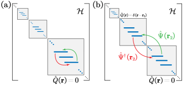
Figure 1: Schematic of gauge invariance (a) and violation (b) spectroscopy. The blocks represent different gauge sectors labeled by $\hat{Q}(\mathbf{r})$ in Hilbert space. In the gauge violation case (b), the operations $\hat{\Psi}(\mathbf{r}_{2}),\hat{\Psi}^{\dagger}(\mathbf{r}_{2})$ induce a transition between $\hat{Q}=0$ and $\hat{Q}=\delta(\mathbf{r}-\mathbf{r}_{2})$ gauge sectors.

Concept. We know that the single-particle absorbing and emission spectrum function can be obtained from the Fourier transformation of the following Green’s functions

$$\mathcal{A}_{\mathrm{ab}}(\mathbf{k},\omega) = i\int dt\int d\mathbf{r}g_{\mathbf{r}}^{>}(t)e^{-i(\mathbf{k\cdot r}-\omega t)},$$ (1)

$$\mathcal{A}_{\mathrm{em}}(\mathbf{k},\omega) = i\varepsilon\int dt\int d\mathbf{r}g_{\mathbf{r}}^{<}(t)e^{-i(\mathbf{k\cdot r}-\omega t)}.$$ (2)

These Green’s functions are defined as

$$ig_{\mathbf{r}_{2}-\mathbf{r}_{1}}^{>}(t) = \left\langle\psi_{0}\right|\hat{\Psi}(\mathbf{r}_{2},t)\hat{\Psi}^{{\dagger}}(\mathbf{r}_{1},0)\left|\psi_{0}\right\rangle,$$ (3)

$$ig_{\mathbf{r}_{2}-\mathbf{r}_{1}}^{<}(t) = \varepsilon\left\langle\psi_{0}\right|\hat{\Psi}^{{\dagger}}(\mathbf{r}_{1},0)\hat{\Psi}(\mathbf{r}_{2},t)\left|\psi_{0}\right\rangle,$$ (4)

where $\hat{\Psi}(\mathbf{r},t)=e^{iHt}\hat{\Psi}(\mathbf{r)}e^{-iHt}$ is the matter field operator in Heisenberg picture, and $\varepsilon=+1(-1)$ for Bosonic (Fermionic) matter field. Here we choose $\left|\psi_{0}\right\rangle$ to be the ground state in the physical sector, i.e. the sector with vanishing gauge charge $\hat{Q}(\mathbf{r})=0$. These Green functions describe the process that adding one particle (hole) to the system at position $\mathbf{r}_{1}$, and removing one particle (hole) at position $\mathbf{r}_{2}$ after evolution time $t$. In synthetic gauge theories, the gauge field can not adjust to follow the charge we add (remove). Thus this process violates the Gaussian law, and excites the system away from the physical sector. More specifically, the matter field operator is not invariant under a local gauge transformation, thus $\left[\hat{\Psi}\left(\mathbf{r}^{\prime}\right),\hat{Q}(\mathbf{r})\right]\neq 0$. One finds $\hat{Q}(\mathbf{r})\hat{\Psi}^{\left({\dagger}\right)}\left(\mathbf{r}^{\prime}\right)\left|\psi_{0}\right\rangle=\pm e\delta(\mathbf{r}-\mathbf{r}^{\prime})\hat{\Psi}^{\left({\dagger}\right)}\left(\mathbf{r}^{\prime}\right)\left|\psi_{0}\right\rangle$. Note that the state $\hat{\Psi}^{\left({\dagger}\right)}\left(\mathbf{r}^{\prime}\right)\left|\psi_{0}\right\rangle$ is no longer in the physical sector as shown in Fig.1(b). Then the Green’s functions can be simplified into

$$ig_{\mathbf{r}_{2}-\mathbf{r}_{1}}^{>}(t) = \delta(\mathbf{r}_{2}-\mathbf{r}_{1}\mathbf{)}\left\langle\psi_{0}\right|\hat{\Psi}(\mathbf{r}_{2}\mathbf{)}e^{-i\hat{H}_{-}t}\hat{\Psi}^{{\dagger}}(\mathbf{r}_{1})\left|\psi_{0}\right\rangle,$$ (5)

$$ig_{\mathbf{r}_{2}-\mathbf{r}_{1}}^{<}(t) = \varepsilon\delta(\mathbf{r}_{2}-\mathbf{r}_{1}\mathbf{)}\left\langle\psi_{0}\right|\hat{\Psi}^{{\dagger}}(\mathbf{r}_{1})e^{+i\hat{H}_{+}t}\hat{\Psi}(\mathbf{r}_{2}\mathbf{)}\left|\psi_{0}\right\rangle.$$ (6)

where $\hat{H}_{\xi}\equiv\hat{H}\left[\hat{Q}(\mathbf{r})=\xi e\delta(\mathbf{r-r}_{1})\right]$, $\xi=\pm$, is the Hamiltonian in the non-physical sectors, and energy of $\left|\psi_{0}\right\rangle$ is set to be zero. Here the delta-function $\delta(\mathbf{r}_{2}-\mathbf{r}_{1}\mathbf{)}$ is due to the fact that if $\mathbf{r}_{2}\neq\mathbf{r}_{1}$, the state will not go back to the physical sector, $\hat{Q}(\mathbf{x})\hat{\Psi}\left(\mathbf{r}_{2}\right)\hat{\Psi}^{{\dagger}}\left(\mathbf{r}_{1}\right)\left|\psi_{0}\right\rangle=\left\{\delta\left(\mathbf{x-r}_{2}\right)-\delta\left(\mathbf{x-r}_{1}\right)\right\}\hat{\Psi}\left(\mathbf{r}_{2}\right)\hat{\Psi}^{{\dagger}}\left(\mathbf{r}_{1}\right)\left|\psi_{0}\right\rangle$. As a result, the gauge violation spectrum exhibits no dispersion $\mathcal{A}_{\mathrm{ab/em}}(\mathbf{k},\omega)=$ $\mathcal{A}_{\mathrm{ab/em}}(\omega)$.

In contrast to gauge violation spectroscopy, to calculate the gauge invariant spectrum, one needs bound the matter field operator to the gauge fields $\hat{\Psi}(\mathbf{r)\longrightarrow}\hat{\Psi}(\mathbf{r)}e^{i\int d^{d}x\mathbf{E}_{\mathrm{cl}}(\mathbf{x})\cdot\mathbf{\hat{A}}(\mathbf{x})}$, where $\mathbf{E}_{\mathrm{cl}}(\mathbf{x})$ is a classical electric field satisfying $\nabla\cdot\mathbf{E}_{\mathrm{cl}}(\mathbf{x})=\delta\left(\mathbf{x-r}\right)$. It is invariant under gauge transformation, and commutes with the gauge charge $\left[\hat{Q}(\mathbf{r}),\hat{\Psi}(\mathbf{r}^{\prime}\mathbf{)}e^{i\int d^{d}x\mathbf{E}_{\mathrm{cl}}(\mathbf{x})\cdot\mathbf{\hat{A}}(\mathbf{x})}\right]=0$. We note that in most quantum simulators of synthetic gauge theories, it is hard to perform the gauge invariant spectroscopy. Since it is challenging to excite such highly non-local excitations. Therefore the commonly used techniques, such as RF spectroscopy, probes the gauge violation spectrum rather than gauge invariant spectrum. Furthermore, we will show that the gauge violation spectroscopy can be used to detect the confinement and deconfinement phases in synthetic gauge theories.

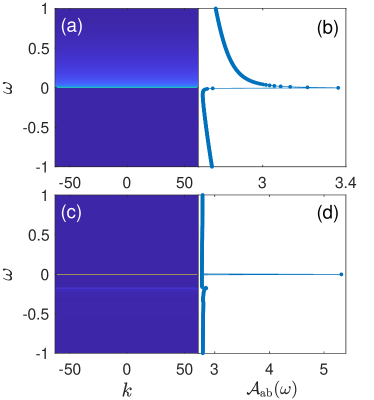
Figure 2: Gauge violation single-particle absorbing spectrum for deconfinement model (a)(b) and for confinement model (c)(d). (a)(c) Momentum resolved gauge violation spectrum. (b)(d) Gauge violation spectrum at a given momentum. We have set coupling constant $g=0.5$ for deconfinement model, and the boson mass $m=e/\sqrt{\pi}=0.17$ for confinement model.

Two Schwinger-like Models. In the following, we will present two one-dimensional models with U(1) local gauge symmetry, which can be both exactly solved via the Bosonization method. One is the celebrated Schwinger model. Its Hamiltonian is given by

$$\hat{H}^{\mathrm{c}}=\hat{H}_{\mathrm{mat}}+\frac{1}{2}\int dx\hat{E}^{2}(x),$$ (7)

where $\hat{H}_{\mathrm{mat}}=\int dx\hat{\Psi}^{{\dagger}}(x)\sigma_{z}[-i\partial_{x}-e\hat{A}(x)]\hat{\Psi}(x)$ and the fermion fields have two components $\hat{\Psi}=(\hat{\Psi}_{R},\hat{\Psi}_{L})^{T}$. The Schwinger model describes the (1+1) dimensional QED Schwinger@1962.I ; Schwinger@1962.II , and exhibits charge confinement phenomena. Another is similar to the Schwinger model. Its Hamiltonian is given by

$$\hat{H}^{\mathrm{d}}=\hat{H}_{\mathrm{mat}}+\frac{u}{2}\int dx\left[\partial_{x}\hat{E}(x)\right]^{2}.$$ (8)

Note that it possesses a modified Maxwell term. The corresponding energy density of gauge field is proportional to the square of electrical field gradient rather than the square of electrical field. This modified Maxwell leads to the deconfinement of charges in this model.

These two models possess the local $U(1)$ gauge symmetries. The corresponding gauge transformation operators are both $\hat{G}=\exp\left\{i\int dx\left[e\hat{\rho}(x)\theta(x)+\hat{E}(x)\partial_{x}\theta\right]\right\}$, where $\theta(x)$ is an arbitrary phase distribution function, and $\hat{\rho}(x)=\hat{\Psi}^{{\dagger}}(x)\hat{\Psi}(x)$ is the particle density operator. Since $\left[\hat{G},\hat{H}^{\mathrm{c(d)}}\right]=0$, the generator of this gauge transformation, $\hat{Q}(x)=\partial_{x}\hat{E}/e-\hat{\rho}(x)$ is a conserved quantity, which is also called gauge charge. In the physical sector, $\hat{Q}(x)=0$, the conservation leads to the Gaussian law in one dimension, $\partial_{x}\hat{E}=e\hat{\rho}(x)$.

We use the Bosonization method to deal with these two models. The Bosonization method maps one dimensional fermions to a problem of bosonic fields Giamarchi@2003.BK . Here both $\hat{H}^{\mathrm{c}}$ and $\hat{H}^{\mathrm{d}}$ can be bosonized in arbitrary gauge sector. As discussed above we only focus on the sector with gauge charge $\hat{Q}(x)=\xi\delta\left(x-x^{\prime}\right)$. The corresponding Bosonized Hamiltonian in these sectors is given by,

$$\hat{H}_{\xi}^{\mathrm{c}} = \hat{H}_{\mathrm{mat}}+\frac{m^{2}}{2}\int dx\left(\phi+\frac{\xi e\mathrm{sgn}\left(x-x^{\prime}\right)}{2m}\right)^{2},$$ (9)

$$\hat{H}_{\xi}^{\mathrm{d}} = \hat{H}_{\mathrm{mat}}+\frac{g}{2}\int dx\left(\partial_{x}\phi+\frac{\xi e\delta\left(x-x^{\prime}\right)}{m}\right)^{2},$$ (10)

where $\hat{H}_{\mathrm{mat}}=\frac{1}{2}\int dx\left[\Pi^{2}+\left(\partial_{x}\phi\right)^{2}\right]$, $g=um^{2}$ and $m^{2}=e^{2}/\pi$. Note that all of these Hamiltonians are quadratic, thus can be exactly diagonalized. Then it is straightforward to calculate the gauge violation correlations defined in Eq. (5,6). For the deconfinement model, one obtains

$$ig^{>}(x,t) = \frac{\delta(x)}{2\pi a}\left(\frac{-ia}{vt-ia}\right)^{\gamma}e^{-iE_{Q}t},$$

$$ig^{<}(x,t) = \frac{\delta(x)}{2\pi a}\left(\frac{ia}{vt+ia}\right)^{\gamma}e^{iE_{Q}t},$$

where $v=\sqrt{1+g}$ and $\gamma=\frac{v^{2}+1}{2v^{3}}$. The ultraviolet cutoff $a$ is introduced by the bosonization procedure, and $E_{Q}$ is an unimportant constant energy. For the Schwinger model, it is hard to obtain a compact analytic form (see supplementary material). Then performing the Fourier transformation one obtains the gauge violation spectral functions.

The results are shown in Figs.2 and 3. Note that for both models, the gauge violation spectrums exhibit no dispersion. For the model with charge confinement, the gauge violation spectrum is a delta function. By contrast, for the deconfined model, the gauge violation spectrum has a finite width. This behavior can be understood as follows: The gauge violation spectroscopy measurement adds one particle with charge $+e$ into the system, add create a gauge charge $-e$ at the same position, which can not move. The interaction between this particle and the gauge charge is governed by electrical field. In the Schwinger model, this interaction energy is proportional to the length of separation between the added particle and the gauge charge, i.e. it is in the confinement phase. Thus the added particle can not move far away from the original position. However, in the deconfinement model, the interaction energy is nearly constant. Then the added particle can move away from the original position. For comparison, we also have calculated the gauge invariance spectroscopy in supplementary material, which exhibit linear dispersion in momentum space.

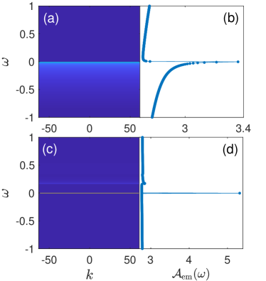
Figure 3: Gauge violation single-particle emission spectrum for deconfinement model (a)(b) and for confinement model (c)(d). (a)(c) Momentum resolved gauge violation spectrum. (b)(d) Gauge violation spectrum at a given momentum. We have set coupling constant $g=0.5$ for deconfinement model, and the boson mass $m=e/\sqrt{\pi}=0.17$ for confinement model.

Quantum Link Model. Recently, the one-dimensional quantum link model, a U(1) lattice gauge theory, has been realized on a quantum simulator based on ultracold bosons in optical lattices YZS@2020.QLM . The Gauss law, as well as the thermalization of this model have been observed Yuan@2022.ETH . By further engineering a tunable topological theta term, the confinement-deconfinement transition has been observed Yuan@2023.angle . The Hamiltonian of the quantum link model is given by Zhai@2022.QLM ; Jad@2023.QLM

$$\hat{H}_{\mathrm{QLM}} = J\sum_{j}\left(\hat{\Psi}_{j+1}^{{\dagger}}\hat{S}_{j+1;j}^{-}\hat{\Psi}_{j}^{{\dagger}}+h.c.\right)$$ (11)

$$+\sum_{j}M\hat{\Psi}_{j}^{{\dagger}}\hat{\Psi}_{j}+\chi\sum_{j}(-1)^{j}\hat{S}_{j+1;j}^{z}.$$

Here the gauge field is represented by spin-1/2 operators $\hat{S}_{i+1;i}^{+}$ on links. $J$ is the gauge-matter coupling strength and $M$ is the mass of the matter field. $\chi$ can tune the topological theta angle $\theta$. When $\chi=0$, $\theta=\pi$, as $\chi\neq 0$, $\theta$ is tuned away from $\pi$. When $\chi\neq 0$, i.e. $\theta$ is away from $\pi$, it is in the confined phase, and no single charge can be observed. When $\chi=0$, i.e. $\theta=\pi$, there is a transition from confined phase to deconfined phase by tuning the matter mass from negative to positive.

The local gauge transformation operator is $\hat{G}_{j}=e^{i\phi\hat{Q}_{j}}$, and the conserved gauge charge is $\hat{Q}_{j}=\hat{S}_{j+1;j}^{z}+\hat{S}_{j;j-1}^{z}+\hat{\Psi}_{j}^{{\dagger}}\hat{\Psi}_{j}$. We calculate the gauge violation spectrum by numerical exact diagonalization. The results of numerical simulation are shown in Fig.4. In Figs.4(a-b), we observe the deconfinement behavior with $M=10J$ and the topological angle $\theta=\pi$. The spectrum has a finite width. Instead, Fig.4(c-d) shows the confinement behavior with $M=-10J,\theta=\pi$. It shows the delta function behavior. This difference clearly distinguishes confinement from deconfinement phase. In Fig.4(c-d), we also observe the same delta function behavior with $M=\pm 10J,\theta\neq\pi$, because there is only a confinement phase when $\theta\neq\pi$.

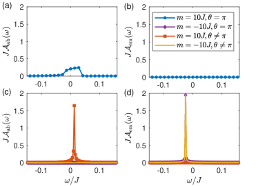
Figure 4: Gauge violation spectroscopies for the one-dimensional quantum link model. (a)(b) Results for deconfinement phase with $M=10J,\theta=\pi$. (c)(d) Results for confinement phase with $M=-10J,\theta=\pi$ and $M=\pm 10J,\theta=\pi/2$. The model contains total number of sites $L=20$.

Summary. We propose the gauge violation spectroscopy in synthetic gauge theories on quantum simulators, which could be used to detect the confinement phase or deconfinement phase. In most single-particle spectroscopy of synthetic gauge theories, such as RF spectroscopy in ultracold quantum gases, one measured the gauge violation spectrum, rather than the gauge invariant spectrum. Since later spectroscopy needs highly non-local perturbations. We used three one-dimensional models with local U(1) gauge symmetry to show that in the confined phase, gauge violation spectrum is nearly a delta-function, while in the deconfinement phase the spectrum has a finite width. However, our conclusions are not limited to one-dimensional models with U(1) gauge symmetry. It can be applied to higher dimensions or non-Abelian gauge. In addition, we would like to point out that, for some simulators, people realize the projected Hamiltonian instead of the Hamiltonian in the full Hilbert space Surace@2020.LGT . In this situation, there is no room for fluctuation of gauge charge. Thus the gauge violation spectroscopy can not be applied in these simulators.

Acknowledgements. We thank Hui Zhai and Yanting Cheng for discussion. This work is supported by Innovation Program for Quantum Science and Technology (Grant No. 2021ZD0302000).

I Schwinger-Like Models

In this supplementary material, we begin by reviewing the Schwinger model with massless fermion, which contains a confinement phase, and presenting a deconfinement model that is similar to the Schwinger model but possesses a modified Maxwell term.

Schwinger-Like Models. In the following we present two one-dimensional models with U(1) local gauge symmetry, the celebrated Schwinger model and deconfinement model with a modified Maxwell term denoted by $\hat{H}^{\mathrm{c}},\hat{H}^{\mathrm{d}}$ respectively,

$$\hat{H}^{\mathrm{c}} = \hat{H}_{\mathrm{mat}}+\frac{1}{2}\int dx\hat{E}^{2}(x),$$ (12)

$$\hat{H}^{\mathrm{d}} = \hat{H}_{\mathrm{mat}}+\frac{u}{2}\int dx\left[\partial_{x}\hat{E}(x)\right]^{2}.$$ (13)

where $\hat{H}_{\mathrm{mat}}=\int dx\hat{\Psi}^{{\dagger}}(x)\sigma_{z}[-i\partial_{x}-e\hat{A}(x)]\hat{\Psi}(x)$ and the fermion fields have two components $\hat{\Psi}=(\hat{\Psi}_{R},\hat{\Psi}_{L})^{T}$. The (anti-)commutation relations are

$$\left\{\hat{\Psi}_{\alpha}(x),\hat{\Psi}_{\beta}^{\dagger}(y)\right\} =\delta_{\alpha\beta}\delta(x-y),$$ (14)

$${\left[\hat{A}(x),\hat{E}(y)\right]} =-i\delta(x-y),$$

with all other (anti-)commutators vanishing.

These two models possess the local U(1) gauge symmetries. Quantum mechanically, the gauge transformation of the two models is implemented by the same unitary operator

$$\hat{G}= \exp\left\{i\int dx\left[e\hat{\rho}(x)\theta(x)+\hat{E}(x)\partial_{x}\theta(x)\right]\right\}$$ (15)

$$= \exp\left\{ie\int dx\left[\hat{\rho}(x)-\frac{1}{e}\partial_{x}\hat{E}(x)\right]\theta(x)\right\},$$

that act as $\hat{G}\hat{\Psi}(x)\hat{G}^{{\dagger}}=\hat{\Psi}(x)e^{-ie\theta(x)}$ and $\hat{G}(x)\hat{A}(x)\hat{G}^{{\dagger}}=\hat{A}(x)-\partial_{x}\theta(x),$ where $\theta(x)$ is an arbitrary phase distribution function, and $\hat{\rho}(x)=\hat{\Psi}^{{\dagger}}(x)\hat{\Psi}(x)$ is the particle density operator. Since the two Hamiltonians (12)(13) are invariant under the gauge transformation, i.e., $\hat{G}\hat{H}^{\mathrm{c(d)}}\hat{G}^{{\dagger}}=\hat{H}^{\mathrm{c(d)}},$ we can conclude that

$$\partial_{x}\hat{E}(x)=e\left(\hat{\rho}(x)+\hat{Q}(x)\right),$$ (16)

where the conserved quantity $\hat{Q}(x)$ is local gauge charge separating the Hamiltonian into different sectors. A physically meaningful state must be invariant to the local gauge transformation and therefore must be annihilated by the operator $\hat{Q}(x)$

$$\hat{Q}(x)|\text{physical state}\rangle=0,$$ (17)

which is nothing but the Gauss’s law analogous to that in three dimension.

For simplicity, we fix a particular gauge such that $\hat{A}(x)$ vanishes. For the purpose, we choose $\partial_{x}\theta(x)=\hat{A}(x)$, then the unitary operator becomes

$$\hat{G} =\exp\left\{i\int dx\left[e\hat{\rho}(x)\int_{-\infty}^{x}\hat{A}(y)dy+\hat{E}(x)\hat{A}(x)\right]\right\}$$ (18)

$$=\exp\left\{i\int dx\left[\hat{A}(x)\int_{x}^{+\infty}e\hat{\rho}(y)dy+\hat{E}(x)\hat{A}(x)\right]\right\}$$

that act as $\hat{G}\hat{\Psi}(x)\hat{G}^{{\dagger}}=\hat{\Psi}(x)e^{-ie\int_{-\infty}^{x}dy\hat{A}(y)},\hat{G}\hat{E}(x)\hat{G}^{\dagger}=2\hat{E}(x)+e\int_{x}^{+\infty}\hat{\rho}(y)dy$ and $\hat{G}\hat{A}(x)\hat{G}^{{\dagger}}=0,$ furthermore,

$$\hat{G}\partial_{x}\hat{E}(x)\hat{G}^{{\dagger}} =2\partial_{x}\hat{E}(x)-e\hat{\rho}(x),$$ (19)

$$\hat{G}\hat{Q}(x)\hat{G}^{\dagger} =2\hat{Q}(x).$$

In the gauge, we arrive at the simplified Hamiltonian

$$\hat{H}^{\mathrm{c}} = \int dx\hat{\Psi}^{{\dagger}}(x)\sigma_{z}[-i\partial_{x}]\hat{\Psi}(x)+\frac{1}{2}\int dx\hat{E}^{2}(x),$$ (20)

$$\hat{H}^{\mathrm{d}} = \int dx\hat{\Psi}^{{\dagger}}(x)\sigma_{z}[-i\partial_{x}]\hat{\Psi}(x)+\frac{u}{2}\int dx\left[\partial_{x}\hat{E}(x)\right]^{2}.$$ (21)

Obviously, the relations $\partial_{x}\hat{E}(x)=e\left(\hat{Q}(x)+\hat{\rho}(x)\right)$ and $[\hat{Q}(x),\hat{H}^{\mathrm{c(d)}}]=0$ are still satisfied by the more compact Hamiltonian.

II Bosonization Method

To calculate the spectral functions, we work out the bosonic version of the Schwinger-like models Eq.(20)(21), which the Bogoliubov transformation can diagonalize in any sector. Before bosonizing the two models, the bosonization dictionary we will use in the following is given,

$$\hat{\Psi}_{R(L)}(x)=\frac{1}{\sqrt{2\pi a}}e^{(-)i\sqrt{4\pi}\hat{\phi}_{R(L)}(x)},$$ (22)

$$\hat{\rho}(x)=\hat{\Psi}_{R}^{{\dagger}}\hat{\Psi}_{R}+\hat{\Psi}_{L}^{{\dagger}}\hat{\Psi}_{L}=\frac{1}{\sqrt{\pi}}\partial_{x}\hat{\phi},$$ (23)

$$\hat{H}_{free}=\int_{-L/2}^{L/2}dx\left[\hat{\Psi}_{R}^{{\dagger}}(x)\left(-i\partial_{x}\right)\hat{\Psi}_{R}(x)+\hat{\Psi}_{L}^{{\dagger}}(x)\left(i\partial_{x}\right)\hat{\Psi}_{L}(x)\right]$$

$$=\frac{1}{2}\int_{-L/2}^{L/2}dx\left[\hat{\Pi}^{2}+\left(\partial_{x}\hat{\phi}\right)^{2}\right],$$ (24)

and some definitions in the above equations

$$\hat{\phi}_{R}(x)=\frac{1}{\sqrt{2L}}\sum_{q}\Theta(+q)\frac{1}{|q|}\left(\hat{b}_{q}e^{iqx}+\hat{b}^{\dagger}_{q}e^{-iqx}\right),$$

$$\hat{\phi}_{L}(x)=\frac{1}{\sqrt{2L}}\sum_{q}\Theta(-q)\frac{1}{|q|}\left(\hat{b}_{q}e^{iqx}+\hat{b}^{\dagger}_{q}e^{-iqx}\right),$$

$$\hat{\phi}=\hat{\phi}_{R}+\hat{\phi}_{L},$$ (25)

$$\hat{\theta}=\hat{\phi}_{L}-\hat{\phi}_{R},$$

$$\hat{\Pi}(x)=\partial_{x}\hat{\theta}(x).$$

where $\hat{b}_{q}$ is the usual bosonic annihilation operator in the state with momentum $q$ satisfying the commutation relations $[\hat{b}_{q},\hat{b}_{q^{\prime}}^{\dagger}]=\delta_{qq^{\prime}}$. $e^{-aq/2}$ is a converging factor with $a\rightarrow 0^{+}$. The system size $L$ will be set to infinity in the last step.

Bosonization. It is straightforward to bosonize the first term in the two models Eq.(20)(21) using the bosonization dictionary Eq.(24). Thus, let’s focus on the second term, which includes the electric field. We can work out the electric field $\hat{E}(x)$ from Gauss’s law (16) using Green’s function method,

$$\hat{E}(x)=\int dy\frac{e}{2}\{\Theta(x-y)-\Theta(y-x)\}(\hat{Q}(y)+\hat{\rho}(x))dy.$$ (26)

Then use the bosonic expression of $\hat{\rho}(x)$ Eq.(23), and straightforward integration leads to

$$\hat{E}(x)=\hat{E}_{B}(x)+\frac{e}{\sqrt{\pi}}\hat{\phi}(x),$$ (27)

where the background electric field generated by the gauge charge $Q(x)$ is defined as

$$\hat{E}_{B}(x)=\int dy\frac{e}{2}\operatorname{sgn}(x-y)\hat{Q}(y)dy.$$ (28)

Take the spatial derivative on both sides of Eq.(27), and we have

$$\partial_{x}\hat{E}(x)=e\hat{Q}(x)+\frac{e}{\sqrt{\pi}}\partial_{x}\hat{\phi}(x).$$ (29)

Substitute Eq.(27) and (29) into Eq.(20) and (21) respectively, and we arrive at the bosonized Hamiltonians in any sector $\hat{Q}(x)$ for the Schwinger-like models,

$$\hat{H}^{\mathrm{c}} = \int dx\frac{1}{2}\left[\hat{\Pi}^{2}+(\partial_{x}\hat{\phi})^{2}+m^{2}\left(\frac{\sqrt{\pi}}{e}\hat{E}_{B}(x)+\hat{\phi}(x)\right)^{2}\right],$$ (30)

$$\hat{H}^{\mathrm{d}} = \int dx\frac{1}{2}\left[\hat{\Pi}^{2}+(\partial_{x}\hat{\phi})^{2}+g\left(\sqrt{\pi}\hat{Q}(x)+\partial_{x}\hat{\phi}\right)^{2}\right]$$ (31)

with the mass of the bosonic field $\hat{\phi}$, $m^{2}=\frac{e^{2}}{\pi}$, and a dimensionless coupling constant $g=ue^{2}/\pi$. In sectors $\hat{Q}(x)=\xi\delta(x-x^{\prime})$ with $\xi=0,\pm$, we obtain $\hat{H}^{\mathrm{c(d)}}_{\xi}$ in the main text.

III Spectral functions

In the following, we want to calculate the following types of correlations

$$ig_{\sigma}^{>}(x,t) = \left\langle\psi_{0}\left|\hat{\Psi}_{R}(x)e^{-i\hat{H}_{\xi}^{\sigma}t}\hat{\Psi}_{R}^{\dagger}(0)\right|\psi_{0}\right\rangle e^{+iE_{0}^{\sigma}t},$$ (32)

$$ig_{\sigma}^{<}(x,t) = \left\langle\psi_{0}\left|\hat{\Psi}_{R}^{\dagger}(0)e^{+i\hat{H}_{\xi}^{\sigma}t}\hat{\Psi}_{R}(x)\right|\psi_{0}\right\rangle e^{-iE_{0}^{\sigma}t}.$$ (33)

Here, $\hat{H}_{\xi}^{\sigma}$ with $\sigma=\mathrm{c,d}$ denote the Hamiltonians of Schwinger-like models as in the main text or see Eq.(34)(35). The two models can be discussed in a fully parallel and unified fashion by introducing the parameter $\sigma$. The $\left|\psi_{0}\right\rangle$ and $E_{0}^{\sigma}$ are the ground state and energy in the physical sector, $\hat{H}_{\xi=0}^{\sigma}\left|\psi_{0}\right\rangle=E_{0}^{\sigma}\left|\psi_{0}\right\rangle$. Since the right and left movers possess the same physics as the other, we only focus on the right mover in the following.

Firstly, we diagonalize the bosonic Schwinger-like models in sectors $\hat{Q}(x)=\xi\delta(x)$ with $\xi=0,\pm$,

$$\hat{H}_{\xi}^{\mathrm{d}} = \hat{H}_{\mathrm{mat}}+\frac{m^{2}}{2}\int dx\left(\phi+\frac{\xi e\mathrm{sgn}\left(x\right)}{2m}\right)^{2},$$ (34)

$$\hat{H}_{\xi}^{\mathrm{c}} = \hat{H}_{\mathrm{mat}}+\frac{g}{2}\int dx\left(\partial_{x}\phi+\frac{\xi e\delta\left(x\right)}{m}\right)^{2}.$$ (35)

It is important to note that the definition of the bosonic field Eq(25) and the Fourier expansion of $\operatorname{sgn}\left(x\right)=\frac{1}{L}\sum_{k}\frac{2}{ik}e^{ikx}$ allow us to rewrite the Hamiltonians into a unified form in momentum space

$$\hat{H}_{\xi}^{\sigma}=E_{\mathrm{zp}}^{\sigma}+\xi^{2}E_{Q}^{\sigma}+\sum_{q}\left\{\mu_{q}^{\sigma}\hat{b}_{q}^{\dagger}\hat{b}_{q}+\frac{1}{2}\Omega_{q}^{\sigma}\left(\hat{b}_{q}\hat{b}_{-q}+\hat{b}_{-q}^{\dagger}\hat{b}_{q}^{\dagger}\right)+i\xi\lambda_{q}^{\sigma}\left(\hat{b}_{q}-\hat{b}_{q}^{\dagger}\right)\right\}.$$ (36)

Here,

$$\begin{gathered}\left\{\begin{array}[]{l}E_{\mathrm{zp}}^{\mathrm{c}}=\sum_{q}\frac{1}{2}\left(|q|+\frac{m^{2}}{2|q|}\right)\\ E_{\mathrm{zp}}^{\mathrm{d}}=\sum_{q}\frac{1}{2}\left(1+\frac{g}{2}\right)|q|\end{array},\right.\quad\left\{\begin{array}[]{l}E_{Q}^{\mathrm{c}}=\sum_{q}\frac{e^{2}}{2Lq^{2}}\\ E_{Q}^{\mathrm{d}}=\sum_{q}\frac{e^{2}g}{2Lm^{2}}\end{array},\right.\\ \left\{\begin{array}[]{l}\mu_{q}^{\mathrm{c}}=|q|+\frac{m^{2}}{2|q|}\\ \mu_{q}^{\mathrm{d}}=(1+\frac{g}{2})|q|\end{array},\right.\quad\left\{\begin{array}[]{l}\Omega_{q}^{\mathrm{c}}=\frac{m^{2}}{2|q|}\\ \Omega_{q}^{\mathrm{d}}=\frac{g|q|}{2}\end{array},\right.\quad\left\{\begin{array}[]{l}\lambda_{q}^{\mathrm{c}}=\frac{em}{q\sqrt{2L|q|}}\\ \lambda_{q}^{\mathrm{d}}=\frac{egq}{m\sqrt{2L|q|}}\end{array}.\right.\end{gathered}$$ (37)

So the Hamiltonian in the physical sector is given by

$$\hat{H}_{\xi=0}^{\sigma}=E_{\mathrm{zp}}^{\sigma}+\sum_{q}\left\{\mu_{q}^{\sigma}\hat{b}_{q}^{\dagger}\hat{b}_{q}+\frac{1}{2}\Omega_{q}^{\sigma}\left(\hat{b}_{q}\hat{b}_{-q}+\hat{b}_{-q}^{\dagger}\hat{b}_{q}^{\dagger}\right)\right\},$$ (38)

which can be diagonalized by utilizing the Bogoliubov transformation

$$\hat{b}_{q} = u_{q}^{\sigma}\hat{\beta}_{q}-v_{q}^{\sigma}\hat{\beta}_{-q}^{\dagger},$$ (39)

$$\hat{b}_{q}^{\dagger} = u_{q}^{\sigma}\hat{\beta}_{q}^{\dagger}-v_{q}^{\sigma}\hat{\beta}_{-q},$$ (40)

with

$$\left\{\begin{array}[]{l}\left(u_{q}^{\sigma}\right)^{2}=\frac{1}{2}\left(\frac{\mu_{q}^{\sigma}}{\varepsilon_{q}^{\sigma}}+1\right)\\ \left(v_{q}^{\sigma}\right)^{2}=\frac{1}{2}\left(\frac{\mu_{q}^{\sigma}}{\varepsilon_{q}^{\sigma}}-1\right)\end{array}\right.,\quad\left\{\begin{array}[]{l}\varepsilon_{q}^{\mathrm{c}}=\sqrt{|q|^{2}+m^{2}}\\ \varepsilon_{q}^{\mathrm{d}}=\sqrt{1+g}|q|\end{array}.\right.\\$$ (41)

It follows that

$$\hat{H}_{\xi=0}^{\sigma}=E_{0}^{\sigma}+\sum_{q}\varepsilon_{q}^{\sigma}\hat{\beta}^{\dagger}_{q}\hat{\beta}_{q},$$ (42)

where $E_{0}^{\sigma}=E_{\mathrm{zp}}^{\sigma}+E_{\mathrm{LHY}}^{\sigma}$ is the ground state energy in the physical sector, and $E_{\mathrm{LHY}}=\frac{1}{2}\sum_{q}(\varepsilon_{q}^{\sigma}-\mu_{q}^{\sigma})$. In this basis, the Hamiltonians in sectors $\hat{Q}(x)=\xi\delta(x)$ can be rewritten into

$$\hat{H}_{\xi}^{\sigma} =E_{0}^{\sigma}+\xi^{2}E_{Q}^{\sigma}+\sum_{q}\varepsilon_{q}^{\sigma}\hat{\beta}_{q}^{\dagger}\hat{\beta}_{q}+\sum_{q}i\xi\lambda_{q}^{\sigma}\left(u_{q}^{\sigma}-v_{q}^{\sigma}\right)\left(\hat{\beta}_{q}-\hat{\beta}_{q}^{\dagger}\right)$$ (43)

$$=E_{0}^{\sigma}+\xi^{2}\tilde{E}_{Q}^{\sigma}+\sum_{q}\varepsilon_{q}^{\sigma}\left(\hat{\beta}_{q}^{\dagger}+\xi h_{q}^{\sigma*}\right)\left(\hat{\beta}_{q}+\xi h_{q}^{\sigma}\right)$$

with

$$h_{q}^{\sigma} = -i\frac{\lambda_{q}^{\sigma}}{\varepsilon_{q}^{\sigma}}\left(u_{q}^{\sigma}-v_{q}^{\sigma}\right),$$ (44)

$$\tilde{E}_{Q}^{\sigma} = E_{Q}^{\sigma}-\sum_{q}\left(\lambda_{q}^{\sigma}\right)^{2}\left(u_{q}^{\sigma}-v_{q}^{\sigma}\right)^{2}/\varepsilon_{q}^{\sigma}.$$ (45)

To calculate spectral functions, it is also convenient to rewrite the bosonic fields Eq.(22) in terms of the new basis

$$\hat{\Psi}_{R}(x)=\frac{1}{\sqrt{2\pi a}}e^{\sum_{q}\left[\eta_{q}^{\sigma}(x)\hat{\beta}_{q}^{\dagger}-\eta_{q}^{\sigma*}(x)\hat{\beta}_{q}\right]}\hat{F}_{\mathrm{R}}$$ (46)

with

$$\eta_{q}^{\sigma}(x)=i\sqrt{\frac{2\pi}{|q|L}}\left[\Theta(+q)u_{q}^{\sigma}-\Theta(-q)v_{q}^{\sigma}\right]e^{-iqx}.$$ (47)

Gauge Invariance Spectroscopy. Substitute Eq.(42)(46) into the Green’s function Eq.(32), and we obtain

$$ig_{\sigma}^{>}(x,t)=\frac{1}{2\pi a}\left\langle\psi_{0}\right|e^{+\sum_{q}\left[\eta_{q}^{\sigma}(x)\hat{\beta}_{q}^{\dagger}-\eta_{q}^{*\sigma}(x)\hat{\beta}_{q}\right]}e^{-it\sum_{q}\varepsilon_{q}^{\sigma}\hat{\beta}_{q}^{\dagger}\hat{\beta}_{q}}e^{-\sum_{q}\left[\eta_{q}^{\sigma}(0)\hat{\beta}_{q}^{\dagger}-\eta_{q}^{*\sigma}(0)\hat{\beta}_{q}\right]}\left|\psi_{0}\right\rangle,$$ (48)

and $ig_{\sigma}^{<}(x,t)$ is similar. Since we are calculating the correlations for the ground state $\left|\psi_{0}\right\rangle$ of $\hat{H}_{\xi=0}$, we can work out the expression by normal-ordering it using Baker-Hausdorff (BH) formula. For deconfinement model, straightforward algebra gives

$$ig_{\mathrm{d}}^{>}(x,t)=\frac{a^{\frac{(v-1)^{2}}{2v}}}{2\pi}\left(i(x+vt)+a\right)^{-\frac{(v+1)^{2}}{4v}}\left(i(-x+vt)+a\right)^{-\frac{(v-1)^{2}}{4v}},$$ (49)

$$ig_{\mathrm{d}}^{<}(x,t)=\frac{a^{\frac{(v-1)^{2}}{2v}}}{2\pi}\left(i(-x-vt)+a\right)^{-\frac{(v+1)^{2}}{4v}}\left(i(x-vt)+a\right)^{-\frac{(v-1)^{2}}{4v}}.$$ (50)

where $v=\sqrt{1+g}$ with dimensionless coupling constant $g=ue^{2}/\pi$. For confinement model, it gives

$$ig_{\mathrm{c}}^{>}(x,t) = \frac{1}{2\pi a}\exp\left\{-\int_{2\pi/L}^{\infty}dqe^{-aq}\frac{m^{4}}{4q^{2}\varepsilon_{q}^{\mathrm{c}}}\left[\frac{1-e^{-i(qx+\varepsilon_{q}^{\mathrm{c}}t)}}{\left(\varepsilon_{q}^{\mathrm{c}}+q\right)^{2}}+\frac{1-e^{i(qx-\varepsilon_{q}^{\mathrm{c}}t)}}{\left(\varepsilon_{q}^{\mathrm{c}}-q\right)^{2}}\right]\right\},$$ (51)

$$ig_{\mathrm{c}}^{<}(x,t) = \frac{1}{2\pi a}\exp\left\{-\int_{2\pi/L}^{\infty}dqe^{-aq}\frac{m^{4}}{4q^{2}\varepsilon_{q}^{\mathrm{c}}}\left[\frac{1-e^{i(qx+\varepsilon_{q}^{\mathrm{c}}t)}}{\left(\varepsilon_{q}^{\mathrm{c}}+q\right)^{2}}+\frac{1-e^{-i(qx-\varepsilon_{q}^{\mathrm{c}}t)}}{\left(\varepsilon_{q}^{\mathrm{c}}-q\right)^{2}}\right]\right\}.$$ (52)

Then we can calculate the spectral functions using the Fourier transformation. The results are shown in Fig.5, which exhibit linear dispersion in momentum space.

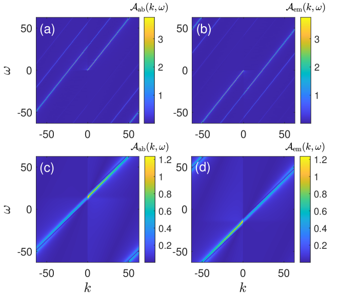
Figure 5: The gauge invariance single-particle absorbing and emission spectrum for deconfinement Model (a)(b) and confinement Model (c)(d). We have set coupling constant $g=0.5$, the mass of boson $m=e/\sqrt{\pi}=0.17$, and system size $L\rightarrow+\infty$.

Gauge Violation Spectroscopy. Because of the orthogonality of states in different gauge sectors, the gauge violation correlations can be written as

$$ig_{\sigma}^{>}(x,t) = \delta(x)\left\langle\psi_{0}\left|\hat{\Psi}_{R}(0)e^{-i\hat{H}_{\xi}^{\sigma}t}\hat{\Psi}_{R}^{\dagger}(0)\right|\psi_{0}\right\rangle e^{+iE_{0}^{\sigma}t},$$ (53)

$$ig_{\sigma}^{<}(x,t) = \delta(x)\left\langle\psi_{0}\left|\hat{\Psi}_{R}^{\dagger}(0)e^{+i\hat{H}_{\xi}^{\sigma}t}\hat{\Psi}_{R}(0)\right|\psi_{0}\right\rangle e^{-iE_{0}^{\sigma}t}.$$ (54)

Substitute Eq.(43)(46) into the above correlations, and we obtain

$$ig_{\sigma}^{>}(x,t)=\frac{\delta(x)}{2\pi a} \left\langle\psi_{0}\right|e^{+\sum_{q}\left[\eta_{q}^{\sigma}(0)\hat{\beta}_{q}^{\dagger}-\eta_{q}^{*\sigma}(0)\hat{\beta}_{q}\right]}e^{-it\sum_{q}\varepsilon_{q}^{\sigma}\left(\hat{\beta}_{q}^{\dagger}+\xi h_{q}^{\sigma*}\right)\left(\hat{\beta}_{q}+\xi h_{q}^{\sigma}\right)}$$ (55)

$$\times e^{-\sum_{q}\left[\eta_{q}^{\sigma}(0)\hat{\beta}_{q}^{\dagger}-\eta_{q}^{*\sigma}(0)\hat{\beta}_{q}\right]}\left|\psi_{0}\right\rangle e^{-i\xi^{2}\tilde{E}_{Q}^{\sigma}t},$$

and $ig_{\sigma}^{<}(x,t)$ is similar. Note that $e^{+\sum_{q}\left[\eta_{q}^{\sigma}(0)\hat{\beta}_{q}^{\dagger}-\eta_{q}^{*\sigma}(0)\hat{\beta}_{q}\right]}$ is a translation operator

$$e^{+\sum_{q}\left[\eta_{q}^{\sigma}(0)\hat{\beta}_{q}^{\dagger}-\eta_{q}^{\sigma*}(0)\hat{\beta}_{q}\right]}\hat{\beta}_{q}^{\dagger}e^{-\sum_{q}\left[\eta_{q}^{\sigma}(0)\hat{\beta}_{q}^{\dagger}-\eta_{q}^{\sigma*}(0)\hat{\beta}_{q}\right]}=\hat{\beta}_{q}^{\dagger}-\eta_{q}^{\sigma*},$$ (56)

$$e^{+\sum_{q}\left[\eta_{q}^{\sigma}(0)\hat{\beta}_{q}^{\dagger}-\eta_{q}^{\sigma*}(0)\hat{\beta}_{q}\right]}\hat{\beta}_{q}e^{-\sum_{q}\left[\eta_{q}^{\sigma}(0)\hat{\beta}_{q}^{\dagger}-\eta_{q}^{\sigma*}(0)\hat{\beta}_{q}\right]}=\hat{\beta}_{q}-\eta_{q}^{\sigma}.$$

Thus we obtain

$$ig_{\sigma}^{>}(x,t)=\frac{\delta(x)}{2\pi a}\left\langle\psi_{0}\right|e^{-it\sum_{q}\varepsilon_{q}^{\sigma}\left(\hat{\beta}_{q}^{\dagger}+\chi_{q}^{\sigma*}\right)\left(\hat{\beta}_{q}+\chi_{q}^{\sigma}\right)}\left|\psi_{0}\right\rangle e^{-i\xi^{2}\tilde{E}_{Q}^{\sigma}t}$$ (57)

with $\chi_{q}^{\sigma}=\xi h_{q}^{\sigma}-\eta_{q}^{\sigma}(0)$. Then, we can define $\hat{B}_{q}^{\sigma}=\hat{\beta}_{q}+\chi_{q}^{\sigma}$, such that $\hat{B}_{q}^{\sigma}\left|\psi_{0}\right\rangle=\chi_{q}^{\sigma}\left|\psi_{0}\right\rangle$. That is to say the ground state $\left|\psi_{0}\right\rangle$ in physical sector is the coherent state of operator $\hat{B}_{q}^{\sigma}$. Thus we have

$$ig_{\sigma}^{>}(x,t) =\frac{\delta(x)}{2\pi a}\left\langle\psi_{0}\left|e^{-it\sum_{q}\varepsilon_{q}^{\sigma}\hat{B}_{q}^{\dagger}\hat{B}_{q}}\right|\psi_{0}\right\rangle e^{-i\xi^{2}\tilde{E}_{Q}^{\sigma}t}$$ (58)

$$=\exp\left\{-i\xi^{2}\tilde{E}_{Q}^{\sigma}t+\sum_{q}\left|\chi_{q}^{\sigma}\right|^{2}\left(e^{-i\varepsilon_{q}^{\sigma}t}-1\right)\right\}$$

Now let us calculate the summation

$$\sum_{q}\left|\chi_{q}^{\sigma}\right|^{2}\left(e^{-i\varepsilon_{q}^{\sigma}t}-1\right)=\sum_{q>0}\frac{2\pi}{|q|L}\gamma_{q,\sigma}^{+}\left(e^{-i\varepsilon_{q}^{\sigma}t}-1\right)+\sum_{q<0}\frac{2\pi}{|q|L}\gamma_{q,\sigma}^{-}\left(e^{-i\varepsilon_{q}^{\sigma}t}-1\right),$$ (59)

where we have defined

$$\gamma_{q,\sigma}^{+} = \left|1+\xi\sqrt{\frac{|q|L}{2\pi}}\frac{\lambda_{q}^{\sigma}}{\varepsilon_{q}^{\sigma}}(u_{q}^{\sigma}-v_{q}^{\sigma})\right|^{2},$$ (60)

$$\gamma_{q,\sigma}^{-} = \left|1+\xi\sqrt{\frac{|q|L}{2\pi}}\frac{\lambda_{q}^{\sigma}}{\varepsilon_{q}^{\sigma}}(v_{q}^{\sigma}-u_{q}^{\sigma})\right|^{2}.$$ (61)

For the deconfinement model, $\gamma_{q,\mathrm{d}}^{+,-}$ is independent of $q$ because of the linearity of the dispersion relation $\varepsilon_{q}^{d}=\sqrt{1+g}|q|$. Thus, we can calculate the summation by using the formula $\ln(1-x)=-\sum_{n>0}x^{n}/n$, and the gauge violation correlations read

$$ig_{\mathrm{d}}^{>}(x,t) = \frac{\delta(x)}{2\pi a}(\frac{-ia}{vt-ia})^{\frac{v^{2}+1}{2v^{3}}},$$ (62)

$$ig_{\mathrm{d}}^{<}(x,t) = \frac{\delta(x)}{2\pi a}(\frac{ia}{vt+ia})^{\frac{v^{2}+1}{2v^{3}}}.$$ (63)

For the confinement model, since $\gamma_{q,\mathrm{c}}^{+,-}$ depends on $q$, it is hard to obtain a compact analytic form. Here, we only show the exponential integral

$$\begin{aligned} ig_{\mathrm{c}}^{>}(x,t)=\frac{\delta(x)}{2\pi a}&\exp\left\{-\int_{2\pi/L}^{\infty}dqe^{-aq}\frac{m^{4}}{4q^{2}\varepsilon_{q}^{\mathrm{c}}}\left[\frac{1-e^{-i\varepsilon_{q}^{\mathrm{c}}t}}{\left(\varepsilon_{q}^{\mathrm{c}}+q\right)^{2}}+\frac{1-e^{-i\varepsilon_{q}^{\mathrm{c}}t}}{\left(\varepsilon_{q}^{\mathrm{c}}-q\right)^{2}}\right]\right\}\\ \times&\exp\left\{+\int_{2\pi/L}^{\infty}dqe^{-aq}\frac{\left(q^{2}+\varepsilon_{q}^{\mathrm{c2}}\right)m^{2}}{2q^{2}\varepsilon_{q}^{\mathrm{c3}}}\left(1-e^{-i\varepsilon_{q}^{\mathrm{c}}t}\right)\right\},\end{aligned}$$ (64)

$$\begin{aligned} ig_{\mathrm{c}}^{<}(x,t)=\frac{\delta(x)}{2\pi a}&\exp\left\{-\int_{2\pi/L}^{\infty}dqe^{-aq}\frac{m^{4}}{4q^{2}\varepsilon_{q}^{\mathrm{c}}}\left[\frac{1-e^{i\varepsilon_{q}^{\mathrm{c}}t}}{\left(\varepsilon_{q}^{\mathrm{c}}+q\right)^{2}}+\frac{1-e^{i\varepsilon_{q}^{\mathrm{c}}t}}{\left(\varepsilon_{q}^{\mathrm{c}}-q\right)^{2}}\right]\right\}\\ \times&\exp\left\{+\int_{2\pi/L}^{\infty}dqe^{-aq}\frac{\left(q^{2}+\varepsilon_{q}^{\mathrm{c2}}\right)m^{2}}{2q^{2}\varepsilon_{q}^{\mathrm{c3}}}\left(1-e^{i\varepsilon_{q}^{\mathrm{c}}t}\right)\right\}.\end{aligned}$$ (65)

After the Fourier transformation, we obtain the gauge violation spectral functions as show in the main text. Here $L=1000$ in Schwinger model, $L\rightarrow\infty$ in deconfinement model and $\alpha=0.01$ for all data have converged the results as illustrated in Fig.6. In the case $m=0$ or $g=0$, the Schwinger-like models reduce to massless Dirac model. All results above are consistent with the known results in the particular case.

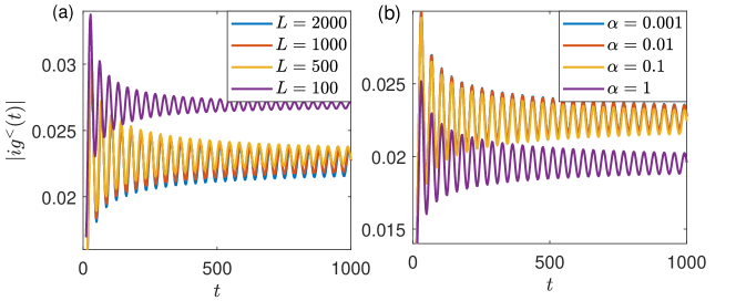
Figure 6: The norm of the gauge violation Green’s function of Schwinger model with $m=0.17$. (a) Results for $L=100,500,1000,2000$ and $\alpha=0.01$. (b) Results for $\alpha=1,0.1,0.01,0.001$ and $L=1000$. We find $L=1000$ and $\alpha=0.01$ have converged the results.

References

• (1) S. Weinberg, The Quantum Theory of Fields, Vol. 2: Modern Applications, (Cambridge University Press, 1995).
• (2) J. Kogut, An introduction to lattice gauge theory and spin systems, Rev. Mod. Phys. 51, 659 (1979).
• (3) E. Fradkin, Field Theories of Condensed Matter Physics, (Cambridge University Press, 2013).
• (4) A. Lopez and E. Fradkin, Fractional quantum Hall effect and Chern-Simons gauge theories, Phys. Rev. B 44, 5246 (1991).
• (5) A. Y. Kitaev, Fault-tolerant quantum computation by anyons, Ann. Phys. 303, 2 (2003).
• (6) C. Schweizer, F. Grusdt, M. Berngruber, L. Barbiero, E. Demler, N. Goldman, I. Bloch and M. Aidelsburger, Floquet approach to $\mathbb{Z}_{2}$ lattice gauge theories with ultracold atoms in optical lattices, Nature Physics 15, 1168 (2019).
• (7) B. Yang, H. Sun, R. Ott, H.-Y. Wang, T. V. Zache, J. C. Halimeh, Z.-S. Yuan, P. Hauke, and J.-W. Pan, Observation of gauge invariance in a 71-site Bose-Hubbard quantum simulator, Nature 587, 392 (2020).
• (8) A. Mil, T. V. Zache, A. Hegde, A. Xia, R. P. Bhatt, M. K. Oberthaler, P. Hauke, J. Berges, and F. Jendrzejewski, A scalable realization of local U(1) gauge invariance in cold atomic mixtures, Science 367, 1128 (2020).
• (9) Z.-Y. Zhou, G.-X. Su, J. C. Halimeh, R. Ott, H. Sun, P. Hauke, B. Yang, Z.-S. Yuan, J. Berges, J.-W. Pan, Thermalization dynamics of a gauge theory on aquantum simulator, Science 377, 6603 (2022).
• (10) H.-Y. Wang, W.-Y. Zhang, Z.-Y. Yao, Y. Liu, Z.-H. Zhu, Y.-G. Zheng, X.-K. Wang, H. Zhai, Z.-S. Yuan, J.-W. Pan, Interrelated thermalization and quantum criticality in a lattice gauge simulator, arXiv:2210.17032
• (11) W.-Y. Zhang, Y. Liu, Y. Cheng, M.-G. He, H.-Y. Wang, T.-Y. Wang, Z.-H. Zhu, G.-X. Su, Z.-Y. Zhou, Y.-G. Zheng, H. Sun, B. Yang, P. Hauke, W. Zheng, J. C. Halimeh, Z.-S. Yuan, J.-W. Pan, Observation of microscopic confinement dynamics by a tunable topological $theta$-angle, arXiv:2306.11794
• (12) E. A. Martinez, C. A. Muschik, P. Schindler, D. Nigg, A. Erhard, M. Heyl, P. Hauke, M. Dalmonte, T. Monz, P. Zoller, and R. Blatt, Real-time dynamics of lattice gauge theories with a few-qubit quantum computer, Nature 534, 516 (2016)
• (13) N. Klco, E. F. Dumitrescu, A. J. McCaskey, T. D. Morris, R. C. Pooser, M. Sanz, E. Solano, P. Lougovski, and M. J. Savage, Quantum-classical computation of Schwinger model dynamics using quantum computers, Phys. Rev. A 98, 032331 (2018).
• (14) N. Klco, M. J. Savage, and J. R. Stryker, SU(2) non-Abelian gauge field theory in one dimension on digital quantum computers, Phys. Rev. D 101, 074512 (2020).
• (15) M. Van Damme, J. C. Halimeh, P. Hauke Gauge-symmetry violation quantum phase transition in lattice gauge theories, arXiv:2010.07338
• (16) J. C. Halimeh, P. Hauke, Reliability of lattice gauge theories, Phys. Rev. Lett. 125, 030503 (2020)
• (17) J. C. Halimeh, V. Kasper, P. Hauke Fate of lattice gauge theories under decoherence, arXiv:2009.07848
• (18) A. Smith, J. Knolle, D. L. Kovrizhin, and R. Moessner, Disorder-Free Localization, Phys. Rev. Lett. 118, 266601 (2017)
• (19) M. Brenes, M. Dalmonte, M. Heyl, and A. Scardicchio, Many-Body Localization Dynamics from Gauge Invariance, Phys. Rev. Lett. 120, 030601 (2017)
• (20) A. Smith, J. Knolle, R. Moessner, and D. L. Kovrizhin, Dynamical localization in Z2 lattice gauge theories, Phys. Rev. B. 97, 245137 (2018)
• (21) J. Osborne, I. P. McCulloch, J. C. Halimeh Disorder-Free Localization in 2+1D Lattice Gauge Theories with Dynamical Matter arXiv:2301.07720 arXiv preprint arXiv:2301.07720
• (22) W. Zheng and P. Zhang, Floquet engineering of a dynamical $Z_{2}$ lattice gauge field with ultracold atoms, arXiv: 2011.01500.
• (23) F. F. Assaad and T. Grover, Simple fermionic model of deconfined phases and phase transitions, Phys. Rev. X, 6, 041049 (2016).
• (24) J. A. Sobota, Y. He, and Z.-X. Shen, Angle-resolved photoemission studies of quantum materials, Rev. Mod. Phys. 93, 025006 (2021)
• (25) Q. Chen, Y. He, C.-C. Chien and K. Levin, Theory of radio frequency spectroscopy experiments in ultracold Fermi gases and their relation to photoemission in the cuprates, Rep. Prog. Phys. 72, 122501 (2009)
• (26) J. T. Stewart, J. P. Gaebler and D. S. Jin, Using photoemission spectroscopy to probe a strongly interacting Fermi gas, Nature 454, 744 (2008).
• (27) C. H. Schunck, Y.-il Shin, A. Schirotzek and W. Ketterle, Determination of the fermion pair size in a resonantly interacting superfluid, Nature 454, 739 (2008).
• (28) P. Wang, Z.-Q. Yu, Z. Fu, J. Miao, L. Huang, S. Chai, H. Zhai, and J. Zhang, Spin-orbit coupled degenerate fermi gases, Phys. Rev. Lett. 109, 095301 (2012).
• (29) L. W. Cheuk, A. T. Sommer, Z. Hadzibabic, T. Yefsah, W. S. Bakr, and M. W. Zwierlein, Spin-Injection Spectroscopy of a Spin-Orbit Coupled Fermi Gas, Phys. Rev. Lett. 109, 095302 (2012)
• (30) Z. Yan, P. B. Patel, B. Mukherjee, R. J. Fletcher, J. Struck and M. W. Zwierlein, Boiling a unitary fermi liquid, Phys. Rev. Lett. 122, 093401 (2019).
• (31) A. Schirotzek, C.-H. Wu, A. Sommer and M. W. Zwierlein, Observation of fermi polarons in a tunable fermi liquid of ultracold atoms, Phys. Rev. Lett. 102, 230402 (2009).
• (32) C. Kohstall, M. Zaccanti, M. Jag, A. Trenkwalder, P. Massignan, G. M. Bruun, F. Schreck and R. Grimm, Metastability and coherence of repulsive polarons in a strongly interacting Fermi mixture, Nature 485, 615 (2012).
• (33) F. Scazza, G. Valtolina, P. Massignan, A. Recati, A. Amico, A. Burchianti, C. Fort, M. Inguscio, M. Zaccanti and G. Roati, Repulsive fermi polarons in a resonant mixture of ultracold 6Li atoms, Phys. Rev. Lett. 118, 083602 (2017).
• (34) N. Jørgensen, L. Wacker, K. Skalmstang, M. Parish, J. Levinsen, R. Christensen, G. Bruun, and J. Arlt, Observation of Attractive and Repulsive Polarons in a Bose-Einstein Condensate, Phys. Rev. Lett. 117, 055302 (2016).
• (35) M.-G. Hu, M. Van de Graaff, D. Kedar, J. P. Corson, E. A. Cornell and D. S. Jin, Bose polarons in the strongly interacting regime, Phys. Rev. Lett. 117, 055301 (2016).
• (36) C. Senko, J. Smith, P. Richerme, A. Lee, W. C. Campbell, C. Monroe, Coherent imaging spectroscopy of a quantum many-body spin system, Science 345, 430 (2014)
• (37) P. Jurcevic, P. Hauke, C. Maier, C. Hempel, B. P. Lanyon, R. Blatt, and C. F. Roos, Spectroscopy of Interacting Quasiparticles in Trapped Ions, Phys. Rev. Lett. 115, 100501 (2015)
• (38) P. Roushan, C. Neill, J. Tangpanitanon, V. M. Bastidas, A. Megrant, R. Barends, Y. Chen, Z. Chen, B. Chiaro, A. Dunsworth, A. Fowler, B. Foxen, M. Giustina, E. Jeffrey, J. Kelly, E. Lucero, J. Mutus, M. Neeley, C. Quintana, D. Sank, A. Vainsencher, J. Wenner, T. White, H. Neven, D. G. Angelakis, J. Martinis, Spectroscopic signatures of localization with interacting photons in superconducting qubits, Science 358, 1175 (2017)
• (39) J. Schwinger, Gauge invariance and mass, Phys. Rev. 125, 397 (1962).
• (40) J. Schwinger, Gauge invariance and mass, II, Phys. Rev. 128, 2425 (1962).
• (41) T. Giamarchi, Quantum Physics in One Dimension, (Oxford University Press 2003),
• (42) Y. Cheng, S. Liu, W. Zheng, P. Zhang and H. Zhai, Tunable confinement-deconfinement transition in an ultracold atom quantum simulator, PRX QUANTUM 3, 040317 (2022).
• (43) J. C. Halimeh, I. P. McCulloch, B. Yang, and P. Hauke, Tuning the Topological $\theta$-Angle in Cold-Atom Quantum Simulators of Gauge Theories, PRX Quantum 3, 040316 (2022).
• (44) F. M. Surace, P. P. Mazza, G. Giudici, A. Lerose, A. Gambassi, and M. Dalmonte, Lattice Gauge Theories and String Dynamics in Rydberg Atom Quantum Simulators, Phys. Rev. X 10, 021041 (2020)