Optical conductivity of a topological system driven using a realistic pulse

Abstract

The effect of a time-periodic perturbation, such as radiation, on a system otherwise at equilibrium has been studied in the context of Floquet theory with stationary states replaced by Floquet states and the energy replaced by quasienergy. These quasienergy bands in general differ from the energy bands in their dispersion and, especially in the presence of spin-orbit coupling, in their states. This may, in some cases, alter the topology when the quasienergy bands exhibit different topological invariants than their stationary counterparts. In this work, motivated by advances in pump-probe techniques, we consider the optical response of driven topological systems when the drive is not purely periodic but is instead multiplied by a pulse shape/envelope function. We use real time-evolved states to calculate the optical conductivity and compare it to the response calculated using Floquet theory. We find that the conductivity bears a memory of the initial equilibrium state even when the pump is turned on slowly and the measurement is taken well after the ramp. The response of the time-evolved system is interpreted as coming from Floquet bands whose population has been determined by their overlap with the initial equilibrium state. In particular, at band inversion points in the Brillouin zone the population of the Floquet bands is inverted as well.

Introduction- The theoretical prediction and experimental realization of topological insulators (TIs) [1, 2, 3, 4, 5, 6, 7, 8, 9] has been one of the greatest developments in condensed matter physics in the last decade. Not only do topological insulators represent a paradigm shift in condensed matter physics, they are also predicted to have a variety of applications [10, 11, 12, 13, 14].

While spin-orbit coupling is a key ingredient, it need not always lead to non-trivial topology as band inversion may not always occur or the presence of a Fermi surface may not be avoided. It has therefore been proposed to use a time-periodic perturbation in order to control the topology [15, 16, 17, 18, 19, 20, 21, 22, 23, 24, 25, 26, 27, 28, 29, 30, 31, 32, 33, 34, 35, 36, 37, 38]. When a time-periodic perturbation is added to a Hamiltonian the system is no longer invariant under an arbitrary translation in time. However a reduced discrete time-translation symmetry still exists. This allows finding solutions to the time-dependent Schrödinger equation using Floquet theory. These solutions or Floquet states are eigenstates of the time evolution operator over a single drive cycle. In other words, Floquet states are periodic up to a phase which is interpreted as $-\epsilon T$ where $\epsilon$ is the quasienergy and $T$ is the drive period. The quasienergies and Floquet states (say, spinors) in general differ from the equilibrium energies and eigenstates respectively. Therefore, along with other properties, topological invariants can change as a result of irradiation leading to driven topological phase transitions. For example, graphene may be driven into a topological phase [31] where gaps appear in the spectrum. In case of Weyl semimetals, Weyl nodes may split into Dirac points or gap out and give rise to Chern bands [39] while spin-orbit coupled insulators are predicted to become topological upon diving [15].

While there are several theoretical predictions, the experimental realization of such Floquet-driven topological phase transitions seems to be challenging. Notably, analogue photonic systems were the first to realize some of these predictions [40] and recently driven graphene has shown signs of topology [41] while the general idea of Floquet bands has been demonstrated by time-resolved ARPES [42, 43].

Several obstacles occur while trying to realize such Floquet-driven topological transitions. These include sample heating, damping and disorder. But perhaps the most elementary deviation from the pure Floquet drive is the unavoidable pulse shape. The drive can not be turned on at time $t=-\infty$ and therefore the state of the system is always connected to that of the equilibrium state. One might expect that at long times after the turning on of the drive, the state will resemble a Floquet state. However, as will be shown below, the notion of adiabaticity does not hold at relevant drive frequencies. In particular, as will be discussed here, the system does not forget its initial conditions. While Floquet states may be a good approximation for the single particle states at long time after the perturbation has been turned on, their population is highly dependent on the initial state. Therefore, one should not expect completely filled or empty Floquet bands at low temperature meaning that the full potential of topological invariance may not be realized. Moreover, it seems that relaxation effects do not necessarily lead to the desired population as the quasienergy is periodic and energy may not necessarily relax to one band [44]. Similarly, when connecting a Floquet spin-Hall insulator to leads, one can not measure quantized conductivity due to mismatch between the equilibrium states of the leads and the driven system [45, 46].

The task at hand is therefore to accurately describe a system driven by a pulse of light whose width is in the range of a few to many time periods, as appropriate for pump-probe techniques and understand the relation between the optical conductivity and Floquet band population. In this work we are interested in the physics of such pump-probe measurements and how topological systems respond to a perturbation that breaks time periodicity. We look at the behavior of the Bernevig-Hughes-Zhang (BHZ) model of a two-dimensional TI [6] in presence of a perturbation in the form of a short pulse and compare it with the response of an exactly periodic (Floquet) drive.

Driven BHZ Model- The equilibrium Hamiltonian in momentum-space is written as

$$H_{0}({\bf k})={\bf d({\bf k})}\cdot{\boldsymbol{\sigma}}$$ (1)

with ${\bf d}({\bf k})=(A\sin k_{x},A\sin k_{y},M-2B(2-\cos k_{x}-\cos k_{y}))$ and ${\boldsymbol{\sigma}}=(\sigma^{x},\sigma^{y},\sigma^{z})$ are the $2\times 2$ Pauli matrices. The mass $M$ and hopping amplitude $B$ are expressed in units of the spin-orbit coupling strength $A$. The spectrum, in general, is insulating in the bulk with a finite band gap. We work in a parameter regime ($M=0.2A$ and $B=0.2A$) where the system is topological. The equilibrium Chern numbers are calculated numerically as explained in the Supplemental material [47] following the method prescribed in Ref [48] and are found to be $C^{Eq}_{\pm}=\pm 1$ for the top and bottom band respectively.

A time-dependence $H(t)=H_{0}+V(t)\sigma^{z}$ effectively makes the mass time-dependent. In the ideal case, $V(t)$ is perfectly periodic with a frequency $\Omega$. However, in reality, this perfect periodicity cannot exist forever and is instead approximated by realistic cases of a slow quench or a Gaussian pulse,

$$V(t)=\begin{cases}V_{{Floq}}(t)=V_{0}\sin(\Omega t)\\ V_{{Pump}}(t)=V_{0}\sin(\Omega t)e^{-\frac{t^{2}}{2\Delta^{2}}}\\ V_{{Quench}}(t)=V_{0}\sin(\Omega t)\frac{1+\tanh(\beta t)}{2}\end{cases}$$ (2)

where $V_{{Floq}},V_{{Pump}}$ and $V_{{Quench}}$ have different envelope functions - constant, Gaussian and a smooth ramp respectively. Here $\beta$ and $\Delta$ are the rate of the quench and the width of the pulse, respectively. $V_{0}$ ($=0.35A$) is the peak amplitude of the perturbation in all cases. The $V_{Floq}(t)$ with frequency $\Omega=2A$ drives the system to a topological phase with Chern numbers $C^{Fl}_{\pm}=\pm 2$.

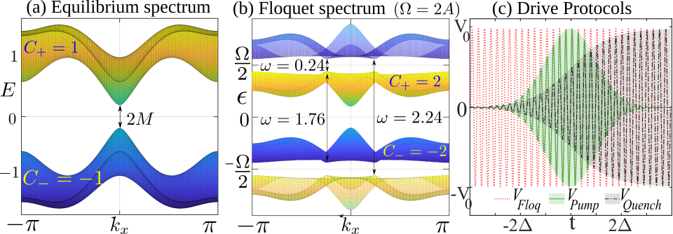
Figure 1: (a) The gapped equilibrium spectrum with Chern number $\pm 1$. (b) With a periodic drive of frequency $\Omega=2A$ the ideal Floquet spectrum is also gapped with Chern numbers $\pm 2$. The transitions marked in (b) correspond to features marked as ${*}$s in Fig. 2. (c) The drive protocols of in Eq. (2) - the ideal Floquet case (red dotted), the slow quench (black dot dash) and the Gaussian pump (green solid) .

In the perfectly periodic case we employ Floquet theory to find the wave functions which are then used to calculate the response functions, assuming that one of the Floquet bands is completely filled while the other is completely empty. In the cases of quench and pump, the analysis requires an actual time evolution over several drive cycles since the perfect periodicity is lost due to the envelope. The response to a non-periodic drive (Gaussian or quench) is calculated using the time-evolved states starting from the equilibrium states of the lower band of the undriven system. We use these states in the Kubo formula as described below.

Linear Response Theory - According to Kubo formula the susceptibility, which is in our case is the response of the driven system to a small probe field is given by,

$$\chi_{AB}(t,t^{\prime})=\lim_{\eta\rightarrow 0^{+}}e^{\eta t^{\prime}}\Big{(} i\Theta(t-t^{\prime}) Tr\Big{\{}g_{0}[A^{I}(t^{\prime}),B^{I}(t)]\Big{\}}$$ (3)

$$+\delta(t-t^{\prime}) Tr\Big{\{}g_{0}M^{I}(t)\Big{\}}\Big{)}$$

where $A^{I}$, $B^{I}$ and $M^{I}$ are operators in the interaction representation. The density matrix $g_{0}$ determines the initial state of the system and $\eta>0$ is a small parameter used to smoothen the response function. The Heaviside step-function $\Theta(t-t^{\prime})$ ensures that causality is not violated. The diamagnetic term $M^{I}(t)$ contributes only to the DC conductivity in the limit $\omega\rightarrow 0$.

For computing electrical conductivity, both $A$ and $B$ are current operators. As explained in the Supplemental material [47], following reference [49], Eq. (3) becomes,

$$\chi_{uv}(t,t^{\prime}) =\lim_{\eta\rightarrow 0^{+}}e^{\eta t^{\prime}}\sum_{\alpha\gamma}g_{0\alpha}\Big{[}2i\Theta(t-t^{\prime})$$ (4)

$$\times \Big{(}\langle\psi_{\alpha}(t^{\prime})|J_{u}|\psi_{\gamma}(t^{\prime})\rangle\langle\psi_{\gamma}(t)|J_{v}|\psi_{\alpha}(t)\rangle-{u\leftrightarrow v}\Big{)}$$

$$+ \delta(t-t^{\prime})\langle\psi_{\alpha}(t)|M_{uv}|\psi_{\alpha}(t)\rangle\Big{]}$$

Here $|\psi_{\alpha}(t))\rangle$ is the state corresponding to band $\alpha$ at time $t$, $g_{0\alpha}$ gives the occupation of states at the initial time; the current operator $J_{u}=\partial_{k_{u}}H$ and the inverse mass $M_{uv}=\partial_{k_{u}}\partial_{k_{v}}H$. The subscripts $u$ and $v$ are the in-plane directions with $u=(\neq)v$ being longitudinal (transverse) conductivity. and the ${\bf k}$-dependence has been skipped for brevity. In the specific case of the model we have considered, the diamagnetic term contributes only to the longitudinal conductivity, since $M_{uv}=0$ identically when $u\neq v$. To obtain the frequency response, we Fourier transform Eq. (4) with respect to the time difference $\tau=t-t^{\prime}$,

$$\chi_{uv}(\omega,t)=\int_{\tau=-\infty}^{\tau=0}d\tau~{}~{}\chi_{uv}(t,t+\tau)e^{-i\omega\tau}.$$ (5)

In general, this depends on the probe time $t$. This is especially important when the perturbation breaks time-periodicity as in the case of a pump-probe experiment and the results are sensitive to the time of measurement. Additionally, we average this over one cycle around $t$ to take into account the small but finite width of the probe,

$$\bar{\chi}_{uv}(\omega,t)=\frac{1}{T}\int_{t}^{t+T}dt^{\prime}\chi_{uv}(\omega,t^{\prime}).$$ (6)

The electrical conductivity is then expressed as

$$\sigma_{uv}(\omega)={\bar{\chi}_{uv}(\omega)}/{\omega}.$$ (7)

Response of a system at equilibrium - For the special case of an unperturbed system, by noting that stationary states evolve as $|\psi_{\alpha}(t)\rangle=e^{-iE_{\alpha}t}|\psi_{\alpha}(0)\rangle$ with $E_{\alpha}$ being the energy of the $\alpha$th band, Eq. (5) becomes,

$$\chi^{Eq}_{uv}(\omega)=i\sum_{\alpha\gamma{\bf k}} g_{0\alpha} \Big{[}\frac{\langle\psi_{\alpha}|H_{u}|\psi_{\gamma}\rangle\langle\psi_{\gamma}|H_{v}|\psi_{\alpha}\rangle}{\omega+(E_{\alpha}-E_{\gamma})+i\eta}$$

$$- \frac{\langle\psi_{\gamma}|H_{u}|\psi_{\alpha}\rangle\langle\psi_{\alpha}|H_{v}|\psi_{\gamma}\rangle}{\omega-(E_{\alpha}-E_{\gamma})+i\eta}\Big{]}$$

$$+\sum_{\alpha{\bf k}} g_{0\alpha} \langle\psi_{\alpha}|M_{uv}|\psi_{\alpha}\rangle.$$ (8)

Note that in the absence of a drive, there is no dependence on the final time $t$ as the system is actually time independent and the averaging in Eq. (6) is skipped.

Response of a perfect Floquet drive - Similarly, we derive a simpler expression for a Floquet system by noting that the Floquet states can be written in terms of the Fourier components $|\phi_{\alpha}^{(n)}\rangle$ i.e.

$$|\Psi_{\alpha}(t)\rangle=e^{-i\epsilon_{\alpha}t}|\phi_{\alpha}(t)\rangle=\sum_{n}e^{-i(\epsilon_{\alpha}-\Omega n)t}|\phi_{\alpha}^{(n)}\rangle$$

$$|\phi_{\alpha}^{(n)}\rangle=\frac{1}{T}\int_{0}^{T}dt~{}e^{-in\Omega t}|\phi_{\alpha}(t)\rangle.$$ (9)

The details of calculating these quasi-mode wavefunctions are given in the Supplemental Material [47]. The expression for the homodyne [49] susceptibility is then modified to,

$$\chi^{Fl}_{uv}(\omega) = i\sum_{\alpha\gamma m{\bf k}}g_{0\alpha}\Bigg{[}\frac{\sum_{l}\langle\phi_{\alpha}^{(l)}|H_{u}|\phi_{\gamma}^{(l+m)}\rangle{\sum_{l^{\prime}}\langle\phi_{\gamma}^{(l^{\prime}+m)}|H_{v}|\phi_{\alpha}^{(l^{\prime})}\rangle}}{\omega+(\epsilon_{\alpha}-\epsilon_{\gamma}-m\Omega)+i\eta}$$ (10)

$$- \frac{\sum_{l}\langle\phi_{\alpha}^{(l)}|H_{v}|\phi_{\gamma}^{(l+m)}\rangle{\sum_{l^{\prime}}\langle\phi_{\gamma}^{(l^{\prime}+m)}|H_{u}|\phi_{\alpha}^{(l^{\prime})}\rangle}}{\omega-(\epsilon_{\alpha}-\epsilon_{\gamma}+m\Omega)+i\eta}\Bigg{]}$$

$$+ \sum_{\alpha{\bf k}l}g_{0\alpha}\langle\phi_{\alpha}^{(l)}|M_{uv}|\phi_{\alpha}^{(l)}\rangle.$$

The terms in the above expression correspond to optical transitions from the $\alpha$ band of the $l$th Floquet zone to the $\gamma$ band of the $(l+m)$th Floquet zone. While in principle the Fourier indices being summed over should span all integers from $-\infty$ to $+\infty$, in practice only a few Fourier components of each state are significant. This can be seen by solving a simpler case of a driven single band system where the weight of the $n$th Fourier mode is proportional to the Bessel function $\mathcal{J}_{n}\left(\frac{V_{0}}{\Omega}\right)$ [45]. For a small ratio $V_{0}/\Omega$ this drops rapidly with $|n|$. In our case we find that $|\phi_{\alpha}^{(n)}\rangle$ is negligible beyond $n=\pm 3$ for the drive parameters that we are working with. Therefore, in order to numerically evaluate the conductivity, we terminate the sums in Eq. (10) at $l=\pm 3$ and $m=\pm 3$. For lower drive frequencies or higher amplitudes a higher cut off may be required.

Importantly, since we assume a perfectly periodic drive we take the population of the levels to have the simple form,

$$g_{0\alpha}=\begin{cases}1&\mbox{for the lower band~{}~{}}(\alpha=-)\\ 0&\mbox{for the upper band~{}~{}}(\alpha=+).\end{cases}$$ (11)

While this is never the case for a driven system, since all drives are turned on at some finite time, many authors resort to this population as it is the simplest.

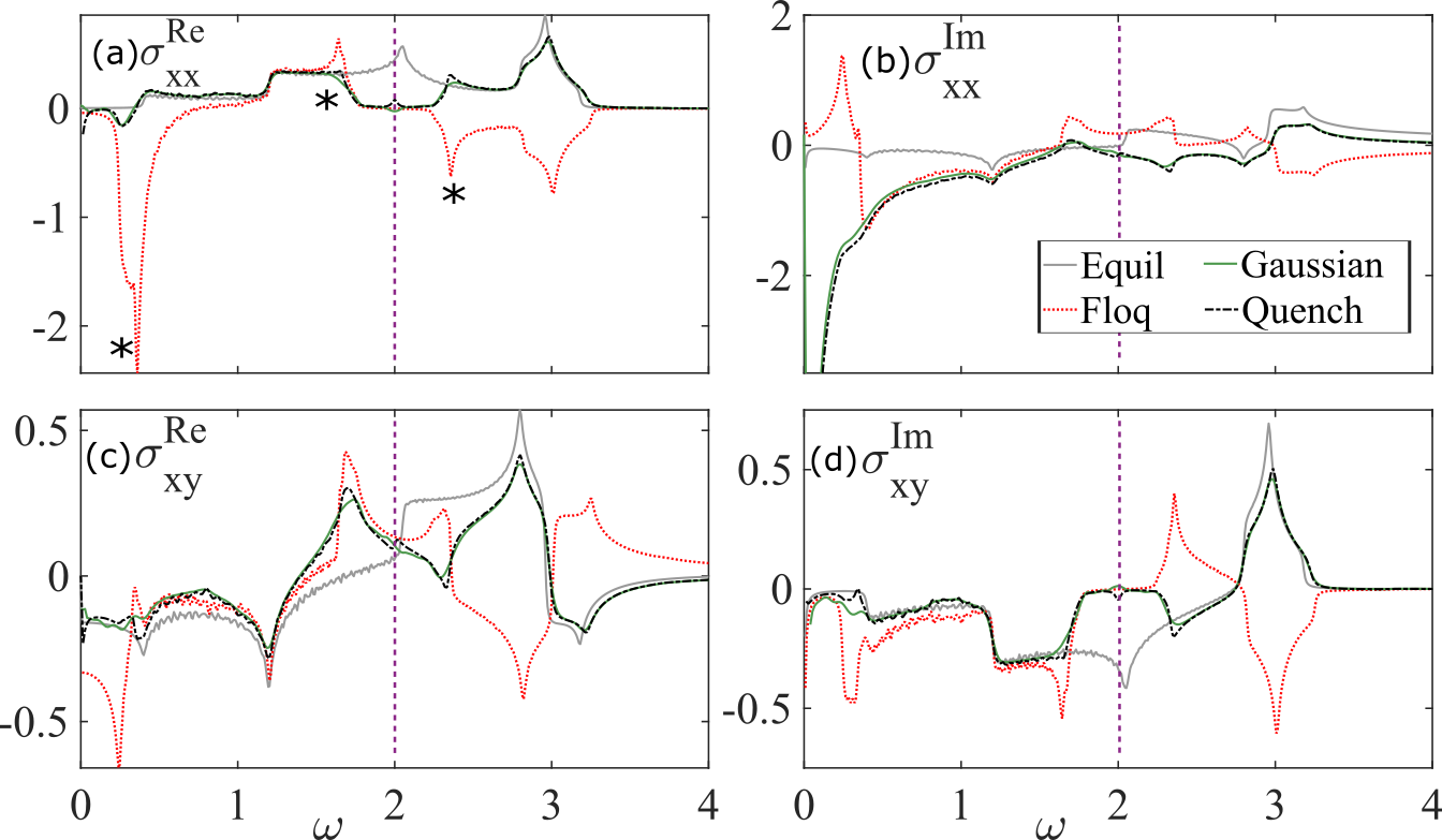
Figure 2: Conductivities for the undriven case (grey solid), pure Floquet drive (red dotted), a Gaussian pump of width $\Delta=20$ cycles (green solid) and a slow quench (black dash-dot) with $\beta=0.05$. As the response to a Gaussian and quench is almost identical, it is safe to infer that the response is almost entirely dependent on the instantaneous drive amplitude.

Gaussian and quench pumps - We now turn our attention to a realistic scenario where the drive is a Gaussian pulse. We first compute the conductivity from Eq. (4) using the real time evolution for a Gaussian pump as well as a quench. We compare that to the response of a perfectly periodic drive as well as the unperturbed (equilibrium) case which are obtained from Eq. (10) and Eq. (8) respectively. For the Floquet response we have used the form of $g_{0\alpha}$ given in Eq. (11).

This comparison is shown in Fig. 2 for $\Omega=2A$ for the real and imaginary parts of longitudinal and transverse conductivity, i.e. (a) $\sigma^{Re}_{xx}$, (b) $\sigma^{Im}_{xx}$, (c) $\sigma^{Re}_{xy}$ and (d) $\sigma^{Im}_{xy}$. The width of the Gaussian is $\Delta=20$ cycles and the quench ramp time is $1/\beta=20$ cycles. The conductivities are shown at the peak of the Gaussian (green solid line) and after the quench has reached saturation (black dot-dash line). Although some features seem to agree, there is a significant difference between the ideal Floquet response and the actual response with a Gaussian drive or a quench. This difference is more pronounced when the probe frequency is higher than the drive frequency, i.e., $\omega>\Omega$ where the sign of certain features is inverted. Moreover, we see that some features which are very strong in the Floquet response are suppressed in the Gaussian/quench response.

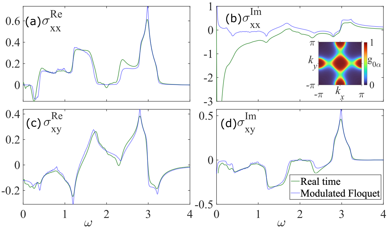
Figure 3: Comparison of the response of a Gaussian evaluated using a real time evolution (green) and the modulated Floquet response (blue) using the $g_{0\alpha}$ in Eq. (12) at the peak of the Gaussian pictured in Fig. 1, when the response is expected to have the most similarity to the ideal Floquet case.

Memory of initial state - The comparison between the response of the periodically driven systems and the ones with a pulse shape leads us to speculate that the initial state is not forgotten even after several cycles of the drive. To illustrate this we devise an approximate expression for the time-evolved conductivity as follows. For a measurement of the Gaussian-driven system at time $\tilde{t}$ we calculate the Floquet states of a system driven by an ideal sinusoidal drive whose amplitude is $V_{{Pump}}(\tilde{t})$. We then use these states to calculate the response using Eq. (10), albeit with one important difference. We replace the simple population $g_{0\alpha}$ of Eq. (11) by the overlap of the Floquet state with the equilibrium state,

$$g_{0\alpha}(\tilde{t})=|\langle\phi_{\alpha}^{\tilde{t}}|\Psi_{0}\rangle|^{2}$$ (12)

where $|\Psi_{0}\rangle$ is the initial state, which in our case we have taken to be lying in the lower band of the equilibrium spectrum. The Floquet state $|\phi_{\alpha}^{\tilde{t}}\rangle$ is the eigenstate of the Floquet operator corresponding to the drive frequency and the instantaneous amplitude, i.e. the magnitude of the envelope function at the probe time $\tilde{t}$. We call the response thus obtained as the “Modulated Floquet response”. The inset in Fig. 3 shows $g_{0\alpha}$ at the peak, with the colors showing the population of the lower band of a given Floquet zone. Here red represents the regions where the lower band is populated and the response in these regions is very close to the Floquet-like response. On the other hand blue is where the upper band is populated and the response is exactly inverted from the Floquet response. Moreover, at the momenta where the original bands have folded to create the Floquet bands, both bands are partially populated. This intermediate regime is responsible for the behaviour around the drive frequency and optical transitions around there are suppressed. This is marked with an asterisk (*) in Figs. 2 and 3 and corresponds to the transitions shown in the Floquet spectrum of Fig. 1(b).

We compare the above “modulated Floquet response” to that of the time evolved system for the case of a Gaussian drive at various probe times (See Supplemental material [47]). The response well before the peak/ramp is found to be close to the equilibrium response, as naturally expected. However, even at the peak of the Gaussian pump $(t=0)$, i.e. where the drive amplitude is the highest, where there is significant mismatch between the time-evolved response and either the Floquet or equilibrium response, the modulated Floquet response gives a good fit. The same holds for the quench scenario, where even though the drive amplitude is kept on for a significantly long time, the response saturates and does not replicate the case of a pure Floquet drive. This means that even when an external driving is switched on very slowly, the system never forgets its initial state and never goes into a pure Floquet regime where only one of the Floquet bands is fully populated.

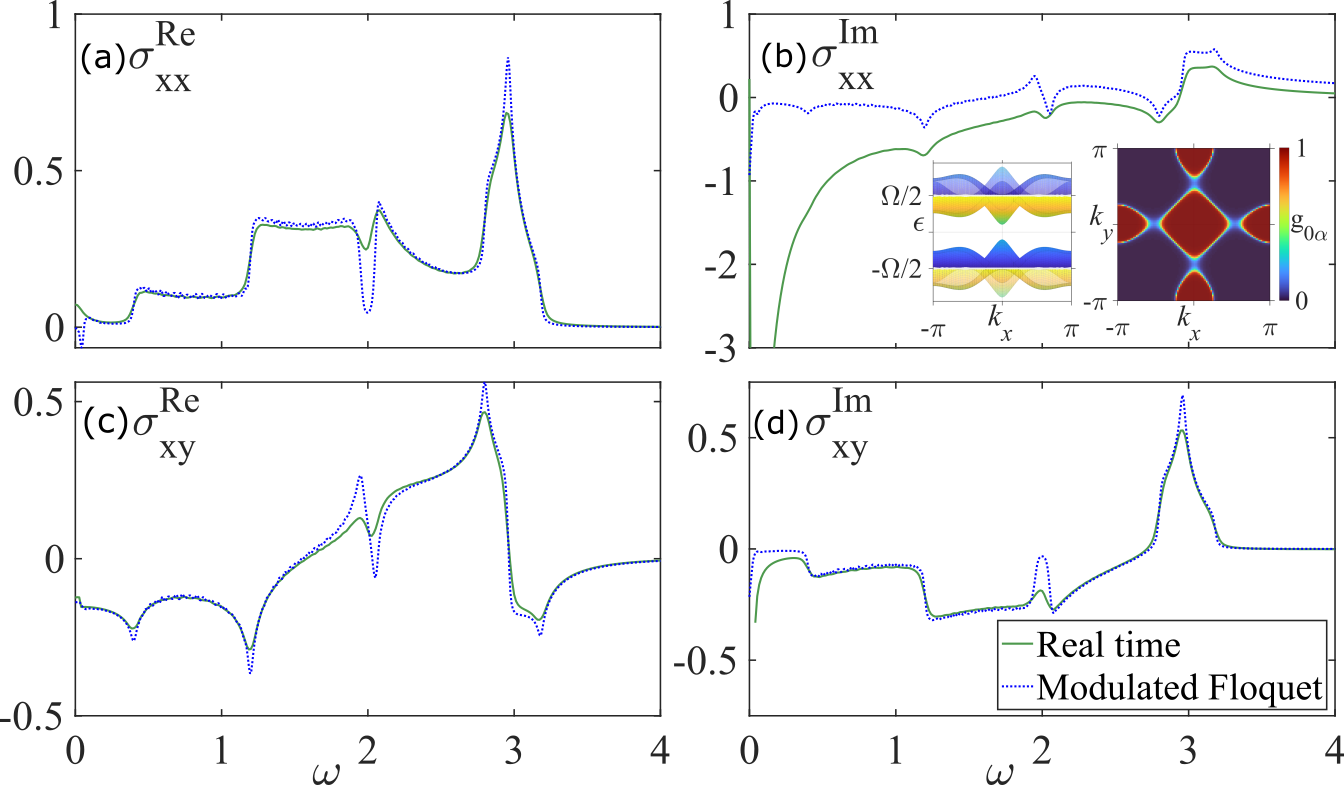
Figure 4: Comparison of the response of a Gaussian evaluated using a real time evolution (green) and the modulated Floquet response (blue) using the $g_{0\alpha}$ in Eq. (12) at $t=-2\Delta$, i.e. well before the peak of the gaussian.

We also plot the response obtained from the real time evolution and the modulated Floquet response for probe time $t=-2\Delta$ in Fig. 4, where, again the two behaviours are in agreement. Similar plots for intermediate probe times and for a higher drive frequency are shown in the Supplemental material [47].

Conclusions - The agreement between the real time evolved conductivity and the modulated Floquet response is a clear sign of the importance of the initial state at any time of probe, even at the center of a wide Gaussian shaped pulse or late after the ramp time of a quench. While the quasi-modes which contribute to the relevant optical transitions can be approximated by an instantaneous Floquet theory, one must keep in mind that band inversion may invert energies but does not invert the population of the bands. This unfortunately means that, unlike at equilibrium, a situation in which quasienergy bands with topological character are not, in general completely full or empty and quantized DC conductivity is not likely.

Acknowledgements - The authors thank Babak Seradjeh and Martin Rodriguez-Vega for useful discussions. We acknowledge financial support from the Natural Sciences and Engineering Research Council of Canada (NSERC) and Fonds de recherche du Québec – Nature et technologies (FRQNT). RS acknowledges Dganit Meidan for financial support from Israel Science Foundation (ISF) grant. The computations presented here were conducted in the computing resources provided by the Digital Research Alliance of Canada and Calcul Quebec.

References

- Moore [2010] J. E. Moore, The birth of topological insulators, Nature 464, 194 (2010).
- Moore and Balents [2007] J. E. Moore and L. Balents, Topological invariants of time-reversal-invariant band structures, Phys. Rev. B 75, 121306 (2007).
- Fu et al. [2007] L. Fu, C. L. Kane, and E. J. Mele, Topological insulators in three dimensions, Phys. Rev. Lett. 98, 106803 (2007).
- Hasan and Kane [2010] M. Z. Hasan and C. L. Kane, Colloquium: Topological insulators, Rev. Mod. Phys. 82, 3045 (2010).
- Qi and Zhang [2011] X.-L. Qi and S.-C. Zhang, Topological insulators and superconductors, Rev. Mod. Phys. 83, 1057 (2011).
- Bernevig et al. [2006] B. A. Bernevig, T. L. Hughes, and S.-C. Zhang, Quantum spin Hall effect and topological phase transition in HgTe quantum wells, Science 314, 1757 (2006).
- Hsieh et al. [2008] D. Hsieh, D. Qian, L. Wray, Y. Xia, Y. S. Hor, R. J. Cava, and M. Z. Hasan, A topological Dirac insulator in a quantum spin hall phase, Nature 452, 970 (2008).
- König et al. [2007] M. König, S. Wiedmann, C. Brüne, A. Roth, H. Buhmann, L. W. Molenkamp, X.-L. Qi, and S.-C. Zhang, Quantum spin Hall insulator state in hgte quantum wells, Science 318, 766 (2007).
- Roth et al. [2009] A. Roth, C. Brüne, H. Buhmann, L. W. Molenkamp, J. Maciejko, X.-L. Qi, and S.-C. Zhang, Nonlocal transport in the quantum spin Hall state, Science 325, 294 (2009).
- Wang et al. [2019] M. Wang, Q. Fu, L. Yan, W. Pi, G. Wang, Z. Zheng, and W. Luo, A topological insulator as a new and outstanding counter electrode material for high-efficiency and endurable flexible perovskite solar cells, ACS Applied Materials & Interfaces 11, 47868 (2019), pMID: 31799822.
- Legg et al. [2022] H. F. Legg, M. Rößler, F. Münning, D. Fan, O. Breunig, A. Bliesener, G. Lippertz, A. Uday, A. A. Taskin, D. Loss, J. Klinovaja, and Y. Ando, Giant magnetochiral anisotropy from quantum-confined surface states of topological insulator nanowires, Nature Nanotechnology 17, 696 (2022).
- Ali Shameli and Yousefi [2022] M. Ali Shameli and L. Yousefi, Light trapping in thin film crystalline silicon solar cells using multi-scale photonic topological insulators, Optics and Laser Technology 145, 107457 (2022).
- Yao et al. [2012] X.-C. Yao, T.-X. Wang, H.-Z. Chen, W.-B. Gao, A. G. Fowler, R. Raussendorf, Z.-B. Chen, N.-L. Liu, C.-Y. Lu, Y.-J. Deng, Y.-A. Chen, and J.-W. Pan, Experimental demonstration of topological error correction, Nature 482, 489 (2012).
- Yue et al. [2016] Z. Yue, B. Cai, L. Wang, X. Wang, and M. Gu, Intrinsically core-shell plasmonic dielectric nanostructures with ultrahigh refractive index, Science Advances 2, e1501536 (2016).
- Lindner et al. [2011] N. H. Lindner, G. Refael, and V. Galitski, Floquet topological insulator in semiconductor quantum wells, Nature Physics 7, 490 (2011).
- Holthaus [2015] M. Holthaus, Floquet engineering with quasienergy bands of periodically driven optical lattices, Journal of Physics B: Atomic, Molecular and Optical Physics 49, 013001 (2015).
- Kundu et al. [2014] A. Kundu, H. A. Fertig, and B. Seradjeh, Effective theory of Floquet topological transitions, Phys. Rev. Lett. 113, 236803 (2014).
- Calvo et al. [2011] H. L. Calvo, H. M. Pastawski, S. Roche, and L. E. F. F. Torres, Tuning laser-induced band gaps in graphene, Applied Physics Letters 98, 232103 (2011).
- Oka and Aoki [2009] T. Oka and H. Aoki, Photovoltaic Hall effect in graphene, Phys. Rev. B 79, 081406 (2009).
- Kitagawa et al. [2010] T. Kitagawa, E. Berg, M. Rudner, and E. Demler, Topological characterization of periodically driven quantum systems, Phys. Rev. B 82, 235114 (2010).
- Rudner et al. [2013] M. S. Rudner, N. H. Lindner, E. Berg, and M. Levin, Anomalous edge states and the bulk-edge correspondence for periodically driven two-dimensional systems, Phys. Rev. X 3, 031005 (2013).
- Nathan and Rudner [2015] F. Nathan and M. S. Rudner, Topological singularities and the general classification of Floquet–Bloch systems, New Journal of Physics 17, 125014 (2015).
- Kitagawa et al. [2011] T. Kitagawa, T. Oka, A. Brataas, L. Fu, and E. Demler, Transport properties of nonequilibrium systems under the application of light: Photoinduced quantum Hall insulators without landau levels, Phys. Rev. B 84, 235108 (2011).
- Tenenbaum Katan and Podolsky [2013] Y. Tenenbaum Katan and D. Podolsky, Generation and manipulation of localized modes in floquet topological insulators, Phys. Rev. B 88, 224106 (2013).
- Titum et al. [2015] P. Titum, N. H. Lindner, M. C. Rechtsman, and G. Refael, Disorder-induced floquet topological insulators, Phys. Rev. Lett. 114, 056801 (2015).
- Fregoso et al. [2013] B. M. Fregoso, Y. H. Wang, N. Gedik, and V. Galitski, Driven electronic states at the surface of a topological insulator, Phys. Rev. B 88, 155129 (2013).
- Foa Torres et al. [2014] L. E. F. Foa Torres, P. M. Perez-Piskunow, C. A. Balseiro, and G. Usaj, Multiterminal conductance of a floquet topological insulator, Phys. Rev. Lett. 113, 266801 (2014).
- Saha [2016] K. Saha, Photoinduced chern insulating states in semi-dirac materials, Phys. Rev. B 94, 081103 (2016).
- Seshadri and Sen [2022] R. Seshadri and D. Sen, Engineering Floquet topological phases using elliptically polarized light, Phys. Rev. B 106, 245401 (2022).
- Seshadri [2023] R. Seshadri, Floquet topological phases on a honeycomb lattice using elliptically polarized light, Materials Research Express 10, 024002 (2023).
- Gu et al. [2011] Z. Gu, H. A. Fertig, D. P. Arovas, and A. Auerbach, Floquet spectrum and transport through an irradiated graphene ribbon, Phys. Rev. Lett. 107, 216601 (2011).
- Harper et al. [2020] F. Harper, R. Roy, M. S. Rudner, and S. Sondhi, Topology and broken symmetry in Floquet systems, Annual Review of Condensed Matter Physics 11, 345 (2020).
- Rudner and Lindner [2020] M. S. Rudner and N. H. Lindner, Band structure engineering and non-equilibrium dynamics in floquet topological insulators, Nature Reviews Physics 2, 229 (2020).
- Lindner et al. [2013] N. H. Lindner, D. L. Bergman, G. Refael, and V. Galitski, Topological Floquet spectrum in three dimensions via a two-photon resonance, Phys. Rev. B 87, 235131 (2013).
- Dóra et al. [2012] B. Dóra, J. Cayssol, F. Simon, and R. Moessner, Optically engineering the topological properties of a spin hall insulator, Phys. Rev. Lett. 108, 056602 (2012).
- Thakurathi et al. [2013] M. Thakurathi, A. A. Patel, D. Sen, and A. Dutta, Floquet generation of majorana end modes and topological invariants, Phys. Rev. B 88, 155133 (2013).
- Thakurathi et al. [2014] M. Thakurathi, K. Sengupta, and D. Sen, Majorana edge modes in the kitaev model, Phys. Rev. B 89, 235434 (2014).
- Katan and Podolsky [2013] Y. T. Katan and D. Podolsky, Modulated Floquet topological insulators, Phys. Rev. Lett. 110, 016802 (2013).
- Hübener et al. [2017] H. Hübener, M. A. Sentef, U. De Giovannini, A. F. Kemper, and A. Rubio, Creating stable floquet–weyl semimetals by laser-driving of 3D Dirac materials, Nature Communications 8, 13940 (2017).
- Rechtsman et al. [2013] M. C. Rechtsman, J. M. Zeuner, Y. Plotnik, Y. Lumer, D. Podolsky, F. Dreisow, S. Nolte, M. Segev, and A. Szameit, Photonic floquet topological insulators, Nature 496, 196 (2013).
- McIver et al. [2020] J. W. McIver, B. Schulte, F.-U. Stein, T. Matsuyama, G. Jotzu, G. Meier, and A. Cavalleri, Light-induced anomalous hall effect in graphene, Nature Physics 16, 38 (2020).
- Farrell et al. [2016] A. Farrell, A. Arsenault, and T. Pereg-Barnea, Dirac cones, floquet side bands, and theory of time-resolved angle-resolved photoemission, Phys. Rev. B 94, 155304 (2016).
- Wang et al. [2013] Y. H. Wang, H. Steinberg, P. Jarillo-Herrero, and N. Gedik, Observation of floquet-bloch states on the surface of a topological insulator, Science 342, 453 (2013).
- Dehghani et al. [2014] H. Dehghani, T. Oka, and A. Mitra, Dissipative Floquet topological systems, Phys. Rev. B 90, 195429 (2014).
- Farrell and Pereg-Barnea [2015] A. Farrell and T. Pereg-Barnea, Photon-inhibited topological transport in quantum well heterostructures, Phys. Rev. Lett. 115, 106403 (2015).
- Farrell and Pereg-Barnea [2016] A. Farrell and T. Pereg-Barnea, Edge-state transport in Floquet topological insulators, Phys. Rev. B 93, 045121 (2016).
- [47] Supplemental material, .
- Fukui et al. [2005] T. Fukui, Y. Hatsugai, and H. Suzuki, Chern numbers in discretized Brillouin zone: Efficient method of computing (spin) hall conductances, Journal of the Physical Society of Japan 74, 1674 (2005).
- Kumar et al. [2020] A. Kumar, M. Rodriguez-Vega, T. Pereg-Barnea, and B. Seradjeh, Linear response theory and optical conductivity of Floquet topological insulators, Phys. Rev. B 101, 174314 (2020).