Bivariate DeepKriging for Large-scale Spatial Interpolation of Wind Fields

Pratik Nag, Ying Sun and Brian J Reich

Some key words: Deep learning, Radial basis function, Bivariate spatial modelling, Non-Gaussian Tukey g-and-h model, Spatial regression, Feature embedding

Short title: Bivariate DeepKriging

1 Introduction

In recent years, Saudi Arabia is seeking to reduce its reliance on fossil fuels for energy demand by investing in renewable energy sources. To achieve this goal, they have introduced several milestones for their upcoming smart cities. For King Abdullah City for Atomic and Renewable Energy (KA-CARE, 2012) they are planning for 54 GW of renewable energy portfolio by 2032, of which 9 GW will come from wind power. The Saudi Vision 2030 (2016) aims at achieving 9.5 GW of renewable energy by 2023. NEOM, an acronym for ”New Future” and ”New Enterprise Operating Model”, is the upcoming mega-city project for Saudi Arabia which is planned to use only renewable power sources (wind and solar). For instance, wind turbines are widely used throughout the world to produce wind energy. However, installing such turbines necessitates precise measurements of the local wind direction and speed. To achieve this goal, an accurate wind speed interpolation model is crucial.

The majority of previous publications modeled wind data using geostatistical methods. Kriging was employed by Wang et al. (2020) to model wind fields. Large wind datasets were modeled for interpolation by Salvaña et al. (2021) using the ExaGeoStat software, which uses bivariate parsimonious Matérn covariance structure. However, these techniques always presumptively assume that the data are stationary and Gaussian. In this paper we propose a novel methodology to model the bivariate wind speed which can then be used for spatial prediction and get high resolution maps of wind fields in any particular region. For our application we have also provided a high resolution wind interpolation for the NEOM region.

Cokriging (Goovaerts, 1998), a multivariate extension of univariate kriging (Cressie, 1990; Stein, 1999), is widely used for analysis and prediction of multivariate spatial fields in multivariate spatial statistics. Prediction (with uncertainty quantification) at new unobserved sites using the information gained from the observed locations is one of the common objectives of this strategy. For Gaussian random fields (Bardeen et al., 1986) with known covariance structure, cokriging is the best linear unbiased predictor. However, in reality, this requirement of Gaussianity and properly stated covariance is rarely met. Because of this, modeling heavy-tailed or skewed data with complicated covariance structure requires a more adaptable prediction methodology.

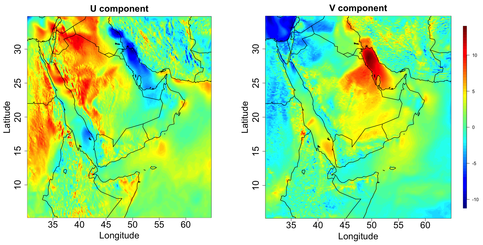
Figure 1: Visualization of the $U$ and $V$ components of the wind field over the Middle East region

Various approaches have been proposed to model non-Gaussian spatial data such as scale mixing Gaussian random fields (Fonseca and Steel, 2011), multiple indicator kriging (Journal and Alabert, 1989), skew-Gaussian processes (Zhang and El-Shaarawi, 2010), copula-based multiple indicator kriging (Agarwal et al., 2021) and Bayesian nonparametrics (Reich and Fuentes, 2015). To address the nonstationary behaviour of the random fields over a large region, non-stationary Matérn covariance models (Nychka et al., 2002; Paciorek and Schervish, 2003; Cressie and Huang, 1999; Fuentes, 2001) have been introduced. Trans-Gaussian random fields (Cressie, 1993; De Oliveira et al., 2002) find nonlinear transformations which enables application of Gaussian processes on the transformed data. However, marginal transformation to normality may not confirm joint normality at multiple locations and may change important properties of the variable (Changyong et al., 2014). One common drawback of many of the approaches is that there is no straight forward implementation of these methods in the bivariate setting and also they may not be optimal for more general spatial datasets. Another issue is that most of these models are based on Gaussian processes which uses cholesky decomposition of the $N\times N$ covariance matrix which requires $\mathbf{O}(N^{3})$ time and $\mathbf{O}(N^{2})$ memory complexity where $N$ is the number of spatial locations.

Recently, Deep neural network (DNN) based algorithms have proved to be the most powerful prediction methodologies in the field of computer vision and natural language processing (LeCun et al., 2015). DNNs can handle more complex functions and in theory they can be applied to approximate any function which is appealing for modelling large-scale nonstationary and non-Gaussian spatial processes. DNNs are also computationally efficient and thus can be applied to large datasets. The computation time for training can be massively reduced by using GPUs (Najafabadi et al., 2015). Due to this broad applicability of the neural networks, several researchers are trying to incorporate DNNs in the spatial problems (Wikle and Zammit-Mangion, 2022). Cracknell and Reading (2014) included spatial coordinates as features for DNNs. Wang et al. (2019) proposed a nearest neighbour neural network approach for Geostatistical modelling. Zammit-Mangion et al. (2021) used neural networks to estimate the warping function which transforms the spatial domain to fit stationary and isotropic covariance structure. Convolutional neural networks (CNNs) (Krizhevsky et al., 2012) can capture the spatial dependence successfully, but require a huge amount of data on regular grid for model training. However, in environmental statistics scenarios one of the main objective is to give spatial interpolation at unobserved locations for irregular grid datasets which is infeasible for CNN modelling. Most of these DNN based methods are developed for univariate data and only concentrate on point predictions and ignore the prediction interval estimations. Recently, there has been few works which proposes density function estimation of the predictive distribution using neural networks, for example Li et al. (2019) proposed a discretized density function approach and predict the predictive distribution probabilities by training a neural network classifier. Neal (2012) and Posch et al. (2019) applied Bayesian inference methodologies to neural networks to predict uncertainties via posterior distributions. But none of these methods are directly applicable to spatial applications.

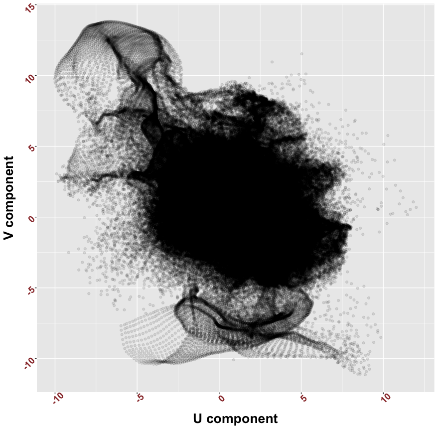
Figure 2: Scatter plot of the $U$ and $V$ components of the Middle Eastern wind field

To address these drawbacks Chen et al. (2022) introduced a spatially dependent deep neural network structure called DeepKriging, for univariate spatial prediction. They used basis functions to capture spatial dependence and use them as features to fit the model. They also provided an approach for uncertainty quantification by an histogram based approach. However, the histograms require thresholds which are mostly deterministic and choice of the thresholds effects the results drastically.

The goal of this paper is to provide a nonparametric statistical framework to perform bivariate spatial prediction and give prediction uncertainties. Our proposed approach, which is a bivariate extension of DeepKriging (Biv.DeepKriging), address these shortcomings. We propose a spatially dependent neural network by adding an embedding layer of spatial coordinates using basis functions. We also propose a bootstrap and ensemble neural network based prediction interval for prediction uncertainty. Biv.DeepKriging is non-parametric, hence it is more general and can be applied to non-Gaussian, nonstationary and even categorical prediction problems. Through simulations we have shown that this approach provides similar results to cokriging when the underlying process is GP and it outperforms traditional statistical methodologies in non-Gaussian and nonstationary scenarios. We have also formulated the deep neural network framework as a nonlinear extension of the linear model of co-regionalization giving a statistical basis for our methodology. Lastly, our proposed approach has been able to reduce the computation time drastically over traditional approaches.

Although architecturally Biv.DeepKriging is a straight forward extension of univarite DeepKriging linking this methodology with traditional statistical methods is still a challenging task. In this paper we have tried to address this by reconstructing Biv.DeepKriging as a nonlinear extension of linear model of co-regionalization.

The rest of our paper is organized as follows. Section 2 introduces the bivariate wind data and examines its non-Gaussian behaviour through some exploratory data analysis. Section 3 gives the proposed methodology. Section 4 compares the performance of the proposed method with traditional approaches. Lastly, Section 5 applies the Biv.DeepKriging method to Saudi Arabian wind data.

2 Exploratory analysis of the wind field data

Wind field estimates play a fundamental role in many applications, such as power generation (Tong, 2010), hydrological modelling (Topaloğlu and Pehlivan, 2018; Millstein et al., 2022) and monitoring and predicting weather patterns and global climate (Arain et al., 2007; Bengtsson and Shukla, 1988). So it is of great interest to get accurate interpolation of wind fields at unobserved locations to exploit the huge potential of wind data for different fields. Wind is generally quantified as a bivariate variable with two components, $U$ and $V$, where $U$ is the zonal velocity, i.e., the component of the horizontal wind towards east and $V$ is the meridional velocity, i.e., the component of the horizontal wind towards north. The wind speed at any location can then be defined as $\sqrt{U^{2}+V^{2}}$.

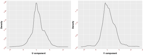
Figure 3: Sample marginal density plots of the $U$ and $V$ components of the Middle Eastern wind data

We analyze wind at $5km\times 5km$ spatial resolution for January, 2009 (1) from a Weather Research and Forecasting (WRF) model simulation on the $[30^{\circ}E,65^{\circ}E]\times[5^{\circ}N,35^{\circ}N]$ region of Earth (Yip, 2018) which spans the Middle East. Figure 1 shows non-stationarity, e.g., the surface is more rough over land than water. The scatter plot in Figure 2 shows a nonlinear relation between the two components. Furthermore, the marginal density plots (Figure 3) of the individual components shows that the data has heavy tails implying non-Gaussianity. Hence, the explanatory analysis provides evidence towards a multivariate non-stationary covariance and non-Gaussian distribution. Traditional Kriging methodologies cannot accomodate these features.

3 Bivariate DeepKriging

3.1 Background

Let $\{\mathbf{Y(\mathbf{s})}=\{Y_{1}(\mathbf{s}),Y_{2}(\mathbf{s})\}^{T},s\in D\},D\subseteq\mathbb{R}^{p}$, be a bivariate spatial process and $\{\mathbf{Z(s_{1})},\mathbf{Z(s_{2})},\\ \cdots,\mathbf{Z(s_{N})}\}$ be the realization of the process at $N$ spatial locations, where $\mathbf{Z(\mathbf{s})}=\{Z_{1}(\mathbf{s}),Z_{2}(\mathbf{s})\}^{T}$. A classical spatial model assumes

$$\mathbf{Z(s)}=\mathbf{Y(s)}+\boldsymbol{\epsilon}(\mathbf{s})$$ (1)

where $\boldsymbol{\epsilon}(\mathbf{s})=\{\epsilon_{1}(\mathbf{s}),\epsilon_{2}(\mathbf{s})\}^{T}$, known as the nugget effect, is a bivariate white noise process with variances $\sigma_{1}^{2}(\mathbf{s})$ and $\sigma_{2}^{2}(\mathbf{s})$ respectively.

Given observations $\mathbf{Z(s)}$, one of the main objectives of spatial prediction is to find the best predictor of the true process $\mathbf{Y(s_{0})}$ at unobserved location $\mathbf{s_{0}}$. The optimal predictor with parameter set $\boldsymbol{\theta}$ can be defined by minimizing the expected value of the loss function, that is,

$$\hat{\mathbf{Y}}^{opt}(\mathbf{s_{0}},\mathbf{Z})=\mathbb{E}\{L(\hat{\mathbf{Y}}(\mathbf{s_{0}}),\mathbf{Y(s_{0})})|\mathbf{Z}_{N}\}=\operatorname*{argmin}_{\boldsymbol{\hat{Y}}}R(\hat{\mathbf{Y}}(\mathbf{s_{0}}),\mathbf{Y(s_{0})}),$$ (2)

where $\hat{\mathbf{Y}}^{opt}(\mathbf{s_{0}},\mathbf{Z})$ is the optimal predictor given $\mathbf{Z}_{N}=\{\mathbf{Z(s_{1})},\mathbf{Z(s_{2})},\cdots,\mathbf{Z(s_{N})}\}$. The function $R(.,.)$ is the risk function is the expected value of the loss $L$.

Bivariate kriging, also known as Cokriging, is the best linear unbiased predictor (Stein and Corsten, 1991; Goovaerts, 1998) for bivariate spatial prediction. The spatial process $\mathbf{Y(s)}$ is typically modeled as

$$\mathbf{Y(s)}=\boldsymbol{\mu}(\mathbf{s})+\boldsymbol{\gamma}(\mathbf{s}),$$ (3)

where $\boldsymbol{\gamma}(\mathbf{s})=\{\gamma_{1}(\mathbf{s}),\gamma_{2}(\mathbf{s})\}$ is a spatially-dependent zero-mean bivariate random process with cross-covariance function $\mathbf{C}_{u,v}(\mathbf{s}_{i},\mathbf{s}_{j})=\text{cov}(\gamma_{u}(\mathbf{s}_{i}),\gamma_{v}(\mathbf{s}_{j}))$, $u,v=1,2$. The mean structure $\boldsymbol{\mu}(\mathbf{s})$ can be modeled as $\boldsymbol{\mu}(\mathbf{s})=\mathbf{X(s)}^{T}\boldsymbol{\beta}$, where $\mathbf{X(s)}=\begin{bmatrix}\mathbf{X}_{1}(\mathbf{s})^{T}&\boldsymbol{0}\\ \boldsymbol{0}&\mathbf{X}_{2}(\mathbf{s})^{T}\end{bmatrix}$, $\mathbf{X}_{u}(\mathbf{s})$ is the $p_{i}\times 1$ vector of covariates for variable $u$, $u=1,2$ and $\boldsymbol{\beta}=\{\boldsymbol{\beta}_{1},\boldsymbol{\beta}_{2}\}^{T}$ is a $(p_{1}+p_{2})\times 1$ vector of coefficients corresponding to the covariates. Let $\mathbf{Z}_{vec}=\{Z_{1}(\mathbf{s_{1}}),...,Z_{1}(\mathbf{s_{N}}),Z_{2}(\mathbf{s_{1}}),...,Z_{2}(\mathbf{s_{N}})\}^{T}$ be a $2N\times 1$ vector, $\mathbf{C}$ is the cross-covariance matrix of order $2N\times 2N$ and $\mathbf{X}=\begin{bmatrix}\{\mathbf{X}_{1}(\mathbf{s}_{1})^{T},...,\mathbf{X}_{1}(\mathbf{s}_{N})^{T}\}^{T}&\boldsymbol{0}\\ \boldsymbol{0}&\{\mathbf{X}_{2}(\mathbf{s}_{1})^{T},...,\mathbf{X}_{2}(\mathbf{s}_{N})^{T}\}^{T}\end{bmatrix}$ is a $2N\times(p_{1}+p_{2})$ matrix of covariates. Then with $\mathbf{V}=(\mathbf{X}^{T}\mathbf{C}^{-1}\mathbf{X})^{-1}$, the kriging prediction at an unobserved location $\mathbf{s_{0}}$ is

$$\hat{\mathbf{Y}}_{vec}(\mathbf{s_{0}})=\mathbf{X_{0}}^{T}\hat{\boldsymbol{\beta}}+\mathbf{C_{0}}^{T}\mathbf{C}^{-1}(\mathbf{Z}_{vec}-\mathbf{X}\hat{\boldsymbol{\beta}})$$ (4)

where $\hat{\boldsymbol{\beta}}=\mathbf{V}\mathbf{X}^{T}\mathbf{C}^{-1}\mathbf{Z}_{vec}$, the generalized least square estimator of $\boldsymbol{\beta}$, $\mathbf{X_{0}}=\mathbf{X}(\mathbf{s}_{0})$ is the $2\times(p_{1}+p_{2})$ matrix of covariates at location $\mathbf{s_{0}}$, $\mathbf{C_{0}}$ is the $2N\times 1$ cross-covariance matrix between the response at location $\mathbf{s_{0}}$ and the observed locations. The choice of cross-covariance functions in cokriging prediction plays a vital role to capture the spatial dependence among locations and also among variables for multivariate data.

Among existing models, multivariate Matérn cross-covariance function (Apanasovich et al., 2012) is one of the most popular class of Matérn covariance function. The flexible Matérn covariance function can be defined as.

$$\mathbf{C}_{u,v}(\mathbf{h})=\sigma_{uv}M\left(\mathbf{h}\middle|\nu_{uv},\sqrt{\alpha_{uv}^{2}}\right),\mathbf{h}=\mathbf{d}(\mathbf{s}_{i},\mathbf{s}_{j})\in\mathbb{R},$$ (5)

where $\mathbf{d}(\mathbf{s}_{i},\mathbf{s}_{j})=\|\mathbf{s}_{i}-\mathbf{s}_{j}\|$ is the Euclidean distance between the locations, $M$ is the Matérn correlation function (Cressie and Huang, 1999), $\nu$ is the smoothness and $\alpha$ is the range parameter. Constraints on these parameters has been derived in Apanasovich et al. (2012).

Another example of cross-covariance function is the linear model of coregionalization (LMC); (Genton and Kleiber, 2015). In this approach, a multivariate random field is represented as a linear combination of $r$ independent random fields with potentially different spatial correlation functions. For $r=2$ we can write the process $\boldsymbol{\gamma}(s)$ in terms of the latent processes as $\boldsymbol{\gamma}(\mathbf{s})=\mathbf{AU(\mathbf{s})}$ where $\mathbf{A}$ is the $2\times 2$ matrix of weights and $\mathbf{U(s)}=\{U_{1}(\mathbf{s}),U_{2}(\mathbf{s})\}^{T},\ \text{cov}(U_{1},U_{2})=0$. Following this architecture the LMC covariance function of a bivariate random field can be written as

$$\mathbf{C}_{ij}(\mathbf{h})=\sum_{k=1}^{r}\rho_{k}(h)A_{ik}A_{jk},\mathbf{h}\in\mathbb{R}^{d},\ 1\leq r\leq 2,$$ (6)

with $\rho_{k}(.)$ as valid stationary correlation functions and $A=(A_{ij})_{i,j=1}^{2,r}$ is a $2\times r$ full rank matrix.

Although co-kriging is the best linear unbiased predictor, it suffers from several limitations. First, maximum likelihood estimation (MLE) for Gaussian processes requires cholesky factorization of the covariance matrix which is computationally expensive making it infeasible to implement traditional co-kriging for large datasets. Moreover, many real life datasets are non-Gaussian and co-kriging is not an optimal predictor in those scenarios.

3.2 DeepKriging for bivariate spatial data

DeepKriging, proposed by Chen et al. (2022), addresses these issues for univariate processes by rephrasing the problem as regression and introducing a spatially dependent neural network structure for spatial prediction. They have used the radial basis functions to embed the spatial locations into a vector of weights and passed them to the DNNs as inputs allowing them to capture the spatial dependence of the process. Similar to Chen et al. (2022), we propose to use spatial basis functions for the bivariate processes to construct the embedding layer instead of passing the coordinates of the observations directly to the NN. This idea is motivated by the multivariate Karhunen-Loéve expansion (Daw et al., 2022) of a multivariate spatial random field, i.e., a p-variate spatial process $\boldsymbol{\gamma(s)}$ can be represented as

$$\boldsymbol{\gamma(s)}=\sum_{b=1}^{\infty}\{w_{b,1}\phi_{b,1}(\mathbf{s}),w_{b,2}\phi_{b,2}(\mathbf{s})\}^{T}$$

where $w_{b,i}$’s are independent random variables and $\phi_{b,i}(s)$’s are the pairwise orthonormal basis functions corresponding to variable $u,u=1,2$. Therefore, a bivariate process can be approximated by

$$\boldsymbol{\gamma}(\mathbf{s})\approx\sum_{b=1}^{K}\{w_{b,1}\phi_{b,1}(\mathbf{s}),w_{b,2}\phi_{b,2}(\mathbf{s})\}^{T},$$

where the weights $w_{b,u}$ can be estimated by minimizing the risk function $R$. Hence the spatial problem can be viewed as multioutput linear regression (Borchani et al., 2015) with these basis functions $\phi_{b,u}$ as covariates.

Among many existing basis functions, such as spline basis functions (Wahba, 1990), wavelet basis functions (Vidakovic, 2009), and radial basis functions (Hastie et al., 2001), we have chosen the multi-resolution compactly supported Wendland radial basis function (Nychka et al., 2015) with the form $w(d)=\frac{(1-d)^{6}}{3}(35d^{2}+18d+13)\mathbf{1}\{0\leq d\leq 1\}$, where $d=\left\|s-u\right\|/\theta$ with $\theta=\frac{1}{2.5\sqrt{u}}$ and anchor point $u\in\{u_{1},u_{2},...,u_{K}\}$. By selecting various $K$ values, one can produce distinct sets of basis functions. This will enable us to record both the long- and short-range spatial dependencies. We must combine these basis functions into a single vector in order to send them to the neural network. See Chen et al. (2022) for detailed discussions on the basis function embedding. Therefore, these co-ordinates embedding can now be used as an input to the DNNs along with covariates $\mathbf{X}_{vec}(\mathbf{s})=\{\mathbf{X}_{1}(\mathbf{s})^{T},\mathbf{X}_{2}(\mathbf{s})^{T}\}^{T}$ which will better capture the spatial features of the data. Note that under our assumption of basis functions, $\phi_{1,u}=\phi_{2,u}$ for location $\mathbf{s}$, hence we can reduce our basis function set to $\boldsymbol{\phi}(\mathbf{s})=\{\phi_{1}(\mathbf{s}),...,\phi_{K}(\mathbf{s})\}^{T}$ where $\phi_{u}(\mathbf{s})=\phi_{1,u}(\mathbf{s}),\ u=1,2,...,K$.

We have used a multi-output deep neural network structure to build the bivariate DeepKriging framework. We define $\mathbf{X}_{\phi}(\mathbf{s})$ as the vector of inputs containing the embedded vector of basis functions $\boldsymbol{\phi}(\mathbf{s})$ and the covariates $\mathbf{X}_{vec}(\mathbf{s})$. Then $\mathbf{X}_{\phi}(\mathbf{s})=(\boldsymbol{\phi}(\mathbf{s})^{T},\mathbf{X}_{vec}(\mathbf{s})^{T})^{T}$. Taking $\mathbf{X}_{\phi}(\mathbf{s})$ as the inputs to a neural network with L layers and $M_{l}$ nodes in layer $l=1,...,L$ DNN can be specified as,

$$h_{1}(\mathbf{X}_{\phi}(\mathbf{s})) =W_{1}\mathbf{X}_{\phi}(\mathbf{s})+b_{1},\ a_{1}(\mathbf{s})=\psi(h_{1}(\mathbf{X}_{\phi}(\mathbf{s})))$$ (7)

$$h_{2}(a_{1}(\mathbf{s})) =W_{2}a_{1}(\mathbf{s})+b_{2},\ a_{2}(\mathbf{s})=\psi(h_{2}(a_{1}(\mathbf{s})))$$

$$..$$ .

$$h_{L}(a_{L-1}(\mathbf{s})) =W_{L}a_{L-1}(\mathbf{s})+b_{L},\ f_{NN}(\mathbf{X}_{\phi}(\mathbf{s}))=h_{L}(a_{L-1}(\mathbf{s})),$$

where $f_{NN}(\mathbf{X}_{\phi}(\mathbf{s}))=\{f_{NN_{1}}(\mathbf{X}_{\phi}(\mathbf{s})),f_{NN_{2}}(\mathbf{X}_{\phi}(\mathbf{s}))\}$ is the prediction output from the model, the weight matrix $W_{l}$ is a $M_{l}\times M_{l-1}$ matrix of parameters and $b_{l}$, a $M_{l}\times 1$ vector is the bias at layer $l$. The parameter set of this network is $\boldsymbol{\theta}=\{W_{l},b_{l}:l=1,2,...,L\}$. $\psi(.)$ signifies the activation function which in our case is the rectified linear unit ReLU (Schmidt-Hieber, 2020). The final layer does not contain any activation function and provides just the linear output allowing it to take any value in $\mathbb{R}^{2}$.

Figure 4 gives a graphical illustration of the spatially dependent neural network structure.

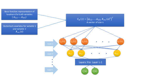
Figure 4: Structure of the spatially dependent neural network with embedding

The Bivariate DeepKriging (Biv.DeepKriging) is a multivariate extension of the univariate DeepKriging. Here we propose to approximate the optimal predictor $\hat{Y}^{opt}(\mathbf{s_{0}})$ with the help of deep neural network structure, i,e; $\hat{Y}^{opt}(\mathbf{s_{0}})\approx f_{NN}(\mathbf{X}_{\phi}(\mathbf{s_{0}}))$ We define the optimal neural network based predictor as $f_{NN}^{opt}(\mathbf{X}_{\phi}(\mathbf{s_{0}}))=\operatorname*{argmin}_{f_{NN}}R(f_{NN}(\mathbf{X}_{\phi}(\mathbf{s_{0}})),\mathbf{Z(s_{0})})$. where $f_{NN}\in\mathcal{F}$ is a multioutput function in the domain of functions $\mathcal{F}$ which are feasible by the defined neural network structure. Here the neural network based functions can be viewed in the parametric form as $f_{NN}(.,\boldsymbol{\theta})$. One can estimate $f_{NN}^{opt}(.)$ by minimizing the empirical version of the risk function $R(.,.)$ based on $\boldsymbol{\theta}$ given as

$$R\{f_{NN}(\mathbf{X}_{\phi}(\mathbf{s}),\theta),\mathbf{Z}_{N}\}=\frac{1}{N}\sum_{n=1}^{N}M(\mathbf{s}_{n}),$$ (8)

where $M(\mathbf{s}_{n})=\frac{w_{1}\times(f_{NN_{1}}(\mathbf{X}_{\phi}(\mathbf{s}))-Z_{1}(\mathbf{s}_{n}))^{2}+w_{2}\times(f_{NN_{2}}(\mathbf{X}_{\phi}(\mathbf{s}))-Z_{2}(\mathbf{s}_{n}))^{2}}{2}.$ and $w_{u}\propto f(\sigma^{2}_{u}),u=1,2$. We have chosen $w_{u}=\frac{1}{\sigma^{2}_{u}}$. Here $\sigma^{2}_{u}$ is unknown and can be estimated through the sample variance of the u-th variable. The final predictor of the neural network would be the bivariate prediction vector $\widehat{f_{NN}}(\mathbf{X}_{\phi}(\mathbf{s_{0}}),\hat{\boldsymbol{\theta}})$ where

$$\hat{\boldsymbol{\theta}}=\operatorname*{argmin}_{\boldsymbol{\theta}}R\{f_{NN}(\mathbf{X}_{\phi}(\mathbf{s}),\boldsymbol{\theta}),\mathbf{Z(s)}\}.$$

3.3 The link between Bivariate DeepKriging and LMC

For univariate case, Chen et al. (2022) proved the link between DeepKriging and Kriging. They showed fixed rank kriging (FRK) (Cressie and Johannesson, 2008), is a linear function of the covariates as well as the basis functions, and thus is a special case of DeepKriging with one layer when all the activation functions are set to be linear.

For the bivariate case, the construction of linear model of coregionalization (LMC) provides some insights on such a link. Using the Karhunen-Loéve Theorem (Adler, 2010), we can write $U_{1}(s)=\sum_{b=1}^{\infty}w_{b,1}\phi_{b,1}(s)$ and $U_{2}(s)=\sum_{b=1}^{\infty}w_{b,2}\phi_{b,2}(\mathbf{s})$ where $w_{b,1}$ and $w_{b,2}$ are elements of $W_{l}$ and $\phi_{b,i}(\mathbf{s})$ is the set of basis functions. Following architecture in (6), the low rank approximation of $\boldsymbol{\gamma}(\mathbf{s})$ can be represented as

$$\boldsymbol{\gamma}(\mathbf{s}) =\mathbf{AU(\mathbf{s})}$$ (9)

$$=\begin{bmatrix}a_{11}\sum_{b=1}^{K}w_{b,1}\phi_{b,1}(\mathbf{s})+a_{12}\sum_{b=1}^{K}w_{b,2}\phi_{b,2}(\mathbf{s})\\ a_{21}\sum_{b=1}^{K}w_{b,1}\phi_{b,1}(\mathbf{s})+a_{22}\sum_{b=1}^{K}w_{b,2}\phi_{b,2}(\mathbf{s})\end{bmatrix}$$

$$=\begin{bmatrix}\sum_{b=1}^{K}(w_{b,1}^{U_{1}}\phi_{b,1}(\mathbf{s})+w_{b,2}^{U_{1}}\phi_{b,2}(\mathbf{s}))\\ \sum_{b=1}^{K}w_{b,1}^{U_{2}}\phi_{b,1}(\mathbf{s})+w_{b,2}^{U_{2}}\phi_{b,2}(\mathbf{s})\end{bmatrix}.$$

So $\boldsymbol{\gamma}(\mathbf{s})$ can be viewed as the linear combination of the two sets of basis functions.

On the other hand with covariate $x(s)=\{1,1,...,1\}^{T}$, $\boldsymbol{\gamma}(s)$ can be represented by the neural network function as $\boldsymbol{\gamma}(s)=f_{NN}(\phi_{1,1}(s),...,\phi_{1,2}(s),...)$. Now in (LABEL:eq:6) with $L=1$ and $\psi(.)$ as the identity function, $f_{NN}(.)$ reduces to

which is the linear combination of the two sets of basis functions. Hence with $L\geq 2$ and with nonlinear activation function $\psi(.)$, the proposed Bivariate DeepKriging is a generalization of the LMC that allows nonlinearity and flexibility to capture more complex spatial dependence.

3.4 Prediction uncertainty

The uncertainty quantification using neural networks has attracted noticeable attention in recent years. Several popular techniques have been developed (Khosravi et al., 2011; Nourani et al., 2021) for better estimation of the prediction interval. For example, Cannon and Whitfield (2002) and Jeong and Kim (2005) used ensemble ANN to form a prediction interval, Srivastav et al. (2007) and Boucher et al. (2009) proposed a bootstrap based uncertainty quantification for DNNs and Kasiviswanathan and Sudheer (2016) proposed a Bayesian framework for the uncertainty quantification with DNNs.

The univariate DeepKriging model on the other hand calculated the prediction interval using an histogram-based approximation to the predictive distribution. However, this method suffers from several limitations. First of all, the prediction interval accuracy heavily depends on the choice of bins for the histogram. The choice of cut points in the histogram which are being randomly chosen from uniform distribution may impact the performance of the approach. The computation time will also go up in training a large number of ensemble models and the ensemble approach proposed by this model may fail to capture the variation in the data. In this section, we will propose an uncertainty quantification method to circumvent these shortcomings.

For the bivariate spatial prediction problem, from (1) and (LABEL:eq:6) we can write $\mathbf{Z(s)}$ in terms of $\mathbf{\hat{Y}(s)}$

$$\mathbf{Z(s)}=\mathbf{\hat{Y}(s)}+{\boldsymbol{\epsilon}}(\mathbf{s})$$ (11)

where ${\boldsymbol{\epsilon}}(\mathbf{s})$ are the residuals $\mathbf{Z(s)}-\mathbf{\hat{Y}(s)}$ with variance-covariance matrix $\begin{bmatrix}{\sigma}_{\epsilon_{1}}^{2}(\mathbf{s})&\mathbf{0}\\ \mathbf{0}&{\sigma}_{\epsilon_{2}}^{2}(\mathbf{s})\end{bmatrix}$. Unlike confidence intervals, prediction intervals quantify the uncertainty associated with each individual prediction location. So, if $\hat{\mathbf{Y}}(\mathbf{s})$ is the prediction for a location $\mathbf{s}$ then the prediction interval considers the deviation of prediction from the true observation, i,e., $\mathbf{Z(\mathbf{s})}-\mathbf{\hat{Y}(\mathbf{s})}=[\mathbf{Y(\mathbf{s})}-\mathbf{\hat{Y}(\mathbf{s})}]+\boldsymbol{\epsilon}(\mathbf{s})$. Assuming the two terms are statistically independent, the variance-covariance matrix associated with $\mathbf{\hat{Y}(\mathbf{s})}$

$$\Sigma_{\mathbf{s}}=\begin{bmatrix}\sigma_{\hat{Y}_{1}}^{2}(\mathbf{s})&cov_{12}(\mathbf{s})\\ cov_{12}(\mathbf{s})&\sigma_{\hat{Y}_{2}}^{2}(\mathbf{s})\end{bmatrix},$$ (12)

where $\sigma_{\hat{Y}_{u}}^{2}(\mathbf{s})$ is the variance of the model outcome and $cov_{12}(\mathbf{s})$ is the covariance between the two variables.

In relation with the above description we propose an ensemble neural network based spatial prediction interval where each model is then trained on randomly selected spatial observations. We divide our training dataset $D$ into two parts $D_{1}$ and $D_{2}$. A sample $D_{11}$ is taken from $D_{1}$.We firstly train one neural network model having L layers with the dataset $D_{11}$, we then take $B$ bootstrap samples from $D_{1}$ and train $B$ DNN models. Note that for these B bootstrap fits we fix the weights of the first $L_{0}$ layers and only allow the new models to be trained based on the last $L-L_{0}$ layers. Now at each location $\mathbf{s}_{k}$ in $D_{2}$, the mean of the predictive distribution can be estimated by averaging over $B$ model outputs.

$$\hat{\mathbf{Y}}_{mean}(\mathbf{s}_{k})=\begin{bmatrix}\frac{1}{B}\sum_{j=1}^{B}\widehat{f_{NN_{1j}}}(\mathbf{X}_{\phi}(\mathbf{s_{k}}))\\ \frac{1}{B}\sum_{j=1}^{B}\widehat{f_{NN_{2j}}}(\mathbf{X}_{\phi}(\mathbf{s_{k}}))\end{bmatrix},$$ (13)

where $\widehat{f_{NN_{uj}}}(\mathbf{X}_{\phi}(\mathbf{s_{0}}))$ is the prediction of $j$-th ensemble model prediction. Now assuming unbiasedness of the NN models $\Sigma_{\mathbf{s}}$ as defined in (12) can be estimated as

Note that $\sigma_{\epsilon_{u}}^{2}(\mathbf{s})$ can be written as

$${\sigma}_{\epsilon_{u}}^{2}(\mathbf{s})=\mathbf{E}\{(Z_{u}(\mathbf{s})-\hat{Y}_{u}(\mathbf{s})\}-\Sigma_{\mathbf{s}_{uu}},\ u=1,2$$ (15)

An empirical approximation of ${\sigma}_{\epsilon_{u}}^{2}$ as defined in 15 is

$$r_{u}^{2}(\mathbf{s})=Max\{(Z_{u}(\mathbf{s})-\hat{Y}_{u}(\mathbf{s}))^{2}-\Sigma_{\mathbf{s}_{uu}},0\},\ u=1,2$$ (16)

Using (16) we calculate $r_{u}^{2}(s_{k})$ which gives the pair $\{s_{k},(r_{1}^{2},r_{2}^{2})\}$. Now to estimate $\sigma_{\epsilon_{u}}^{2}$ at a test location $\mathbf{s}_{0}$ we used the nearest neighbour approach. We obtain a set $D_{20}=\{\mathbf{s}_{k}:\mathbf{s}_{k}\in D_{2}\}$ with cardinality $G$ of locations closest to $\mathbf{s}_{0}$ and take average of the corresponding $r_{u}^{2}$’s, i,e.,

$$\hat{\sigma}_{\epsilon_{u}}^{2}(\mathbf{s}_{0})=\frac{1}{G}\sum_{\mathbf{s}_{g}\in D_{20}}r_{u}^{2}(\mathbf{s}_{g}),$$ (17)

such that $\mathbf{s}_{g}$’s are the nearest $G$ locations to $\mathbf{s}_{0}$.

Now at $\alpha$ level of significance we can write the prediction interval at $\mathbf{s}_{0}$ as

$$\hat{\mathbf{Y}}_{mean_{u}}(\mathbf{s}_{0})\pm t_{(1-\alpha/2),df}\sqrt{\hat{\Sigma}_{\mathbf{s_{0}}_{uu}}+\hat{\sigma}_{\epsilon_{u}}^{2}(\mathbf{s}_{0})},\ u=1,2$$ (18)

where $t_{(1-\alpha/2),df}$ is the $1-\alpha/2$ quantile of $t$-distribution with $df$ degrees of freedom, $df=N-p$, where $p$ is the Number of estimated parameters. Note that for these bootstrap neural networks we have trained only $L-L_{0}$ layers resulting in reduced number of parameters in the modelling. This ensures $df$ to be positive.

Algorithm 1 have provides a step-by-step explanation of our prediction interval construction method.

Algorithm 1 Algorithm for prediction intervals

Split $\mathbf{D}$ in $\mathbf{D_{1}}$ and $\mathbf{D_{2}}$ equally.

Further split $\mathbf{D_{1}}$ into $\mathbf{D_{11}}$ and $\mathbf{D_{12}}$.

Train a DNN of L layers on $\mathbf{D_{11}}$.

Take B random samples $\{\mathbf{D_{1}^{1},D_{1}^{2},...,D_{1}^{B}}\}$ from $\mathbf{D_{1}}$.

for $j\leftarrow 1$ to B do

     Fix the weights of first $L_{0}$ layers of the DNN and train the last $L-L_{0}$ layers on $\mathbf{D_{1}^{j}}$.

     Train the DNN on $\mathbf{D_{1}^{j}}$ and store. Call it $\widehat{f_{NN_{j}}}(\mathbf{X}_{\phi}(\mathbf{s}))$

end for

Average over all predictions based on B DNNs to get the prediction mean (13) at test location $\mathbf{s_{0}}$ $\hat{\mathbf{Y}}_{mean}(\mathbf{s}_{0})$ and variance-covariance matrix $\hat{\Sigma}_{\mathbf{s}_{0}}$

for location $\mathbf{s}_{k}$ in $\mathbf{D_{2}}$ do

     calculate $\hat{\mathbf{Y}}_{mean}(\mathbf{s}_{k})$ and $\hat{\Sigma}_{\mathbf{s}_{k}}$

     calculate $r_{u}^{2}(\mathbf{s}_{k})$ as defined in (16)

end for

For test location $\mathbf{s}_{0}$ obtain the set $\mathbf{D_{20}}=\{\mathbf{s}_{k}:\mathbf{s}_{k}\in\mathbf{D_{2}}\}$ of nearest $G$ locations from $\mathbf{s}_{0}$

calculate $\hat{\sigma}_{\epsilon_{u}}^{2}(\mathbf{s}_{0})$ as defined in (17)

calculate $\hat{\mathbf{Y}}_{mean_{u}}(\mathbf{s}_{0})\pm t_{(1-\alpha/2),df}\sqrt{\hat{\Sigma}_{\mathbf{s_{0}}_{uu}}+\hat{\sigma}_{\epsilon_{u}}^{2}(\mathbf{s}_{0})}$ (18)

$\triangleright$ u stands for i-th variable, u =1,2

3.5 Computational scalability

To better understand the computational benefits of DNN over traditional kriging we can look at the time complexity of the DNN with kriging. DeepKriging involves matrix multiplication in several layers to give us the resulting output. Whereas, kriging involves a $2N\times 2N$ matrix inversion. Note that, time complexity of multiplication of one $m\times n$ and $n\times p$ matrix is $O(mnp)$. So a single layer $l$ of the neural network with minibatch (a minibatch (Hinton et al., 2012) is a randomly selected portion of the data used for neural network training.) size of $b$, $M_{l-1}$ input nodes and $M_{l}$ output nodes will have the time complexity of $O(bM_{l-1}M_{l})$. Faster training is made possible by defining a minibatch. Hence a neural network with $L$ layers will have time complexity $O(\sum_{l=1}^{L}bM_{l-1}M_{l})$. On the other hand, time complexity of Kriging is $O(8N^{3})$. Hence for large $N$ deep kriging with adequate number of layers and nodes is more computationally efficient than traditional kriging.

4 Simulation Studies

4.1 Point predictions

We have conducted several experiments through Gaussian, non-Gaussian and nonstationary simulations to give a comprehensive comparison of our proposed method with the flexible bivariate Matérn (CoKriging.Matérn) as well as the linear model of coregionalization (CoKriging.LMC). In order to compare our results we have computed the Root Mean Square Prediction Error for each variable as the validation metric. For $N$ locations this can be given as

$$\mathbf{RMSPE}_{u}=\sqrt{\frac{1}{N}\sum_{n=1}^{N}(Z_{u}(\mathbf{s_{n}})-\hat{Z_{u}}(\mathbf{s_{n}}))^{2}},\ u=1,2.$$ (19)

The first simulation scenario generates data from a two-dimensional stationary Gaussian process with the parsimonious Matérn covariance function. The simulated data is generated from a zero mean Gaussian Process (GP) with bivariate Matérn covariance having cross-correlation $\rho=0.8$, variances $\sigma_{1}^{2}(\mathbf{s})=0.89\ \text{and}\ \sigma_{2}^{2}(\mathbf{s})=1.3$, smoothness $\nu_{1}=\nu_{2}=0.8$ and range parameters $\alpha_{1}=0.2\ \text{and}\ \alpha_{2}=0.4$. We have generated $50$ replicates with the above parameter configuration on $1200$ equally-spaced locations over $[0,1]\times[0,1]$. We have taken 800 points for training and the rest for testing.

We have taken the following deep neural network structure for modelling.

• We have used $3$ layers of basis functions with $K=25,79,81$ respectively, in total we had $155$ basis functions.

• The Neural network consists of $L=6$ layers with $M_{1}=M_{2}=M_{3}=M_{4}=100$ for first $4$ layers and $M_{5}=50,M_{6}=2$ nodes in the final two layers.

• We initialized the weight matrices by taking samples from normal distribution, we used L1L2 regularizers in the first two layers and chose $0.01$ as the learning rate.

• Through trial and error, we adjusted the number of nodes and layers to give reasonable performance.

Although the nonlinear structure of Biv.DeepKriging captures more specific features from data we still need to validate that our proposal for extending the univariate DeepKriging (Chen et al., 2022) to Bivariate scenario improves the prediction results by exploiting the dependence within the variables. To do this, we compare our proposed model with the univariate DeepKriging model predictions. We compute the average RMSPE independently for each variable over 50 replicates. Table 1 shows that the Bivariate DeepKriging provides better performance in the prediction error than the independent univariate DeepKriging (Indep.DeepKriging) fitted with the same network architecture. We have also the average RMSPE for parsimonious Matérn model with true parameters ($\mathbf{CoKriging.Mat\acute{e}rn}_{true}$). Table 1 shows Biv.DeepKriging performs well enough in comparison with $\mathbf{CoKriging.Mat\acute{e}rn}_{true}$.

Table 1: Comparison of RMSPE for both the variables and its standard error (SE) over different simulation settings.

Simulation type	Models	$\textbf{RMSPE}_{1}$	$\textbf{SE}_{1}$	$\textbf{RMSPE}_{2}$	$\textbf{SE}_{2}$
Gaussian	$\textbf{CoKriging.Mat\'{e}rn}_{true}$ Indep.DeepKriging Biv.DeepKriging	0.23 0.25 0.24	0.91 ($\times 10^{-4}$) 1.21 ($\times 10^{-4}$) 1.33 ($\times 10^{-4}$)	0.21 0.26 0.24	0.93 ($\times 10^{-4}$) 2.32 ($\times 10^{-4}$) 1.17 ($\times 10^{-4}$)
non-Gaussian	CoKriging.Matérn CoKriging.LMC Biv.DeepKriging	9.43 3.98 2.21	1.56 1.59 0.60	7.25 2.87 2.86	0.62 0.57 0.63
non-stationary	CoKriging.Matérn CoKriging.LMC Biv.DeepKriging	0.035 0.036 0.035	2.21 ($\times 10^{-3}$) 2.13 ($\times 10^{-3}$) 1.77 ($\times 10^{-3}$)	0.07 0.07 0.04	3.32 ($\times 10^{-3}$) 6.15 ($\times 10^{-3}$) 2.19 ($\times 10^{-3}$)

Next, we simulate bivariate non-Gaussian random field at 1200 locations on $[0,1]\times[0,1]$ by transforming the Gaussian fields from the previous simulation using the Tukey-g and h transformation (Xu and Genton, 2017) defined as

$$\tau_{g,h}(z)=g^{-1}\{exp(gz)-1\}exp(hz^{2}/2),$$

with $g=0.5,h=1.5$ for variable 1 and $g=-0.4,h=1.3$ for variable 2.

Figure 5 shows the boxplot of RMSPE for the two variables over the 50 replicates. From the boxplots it can be clearly seen that Biv.DeepKriging outperforms other conventional approaches. Note that in some cases, the covariance matrix was singular, which added to the challenges we had when fitting the cokriging models. For our simulation studies we have removed such cases.

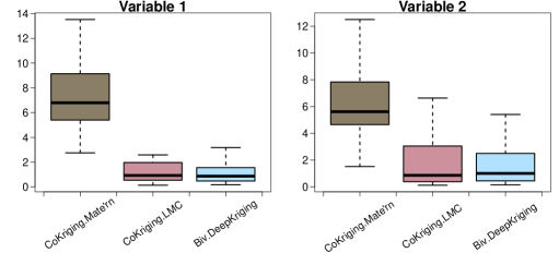
Figure 5: Boxplot of RMSPE for the three different models CoKriging.Matérn, CoKriging.LMC and Biv.DeepKriging over 50 replicates for the non-Gaussian simulation.

The last simulation focuses on two-dimensional data with non-stationary feature. To do so, we followed several computer examples (Ba and Joseph, 2012; Xiong et al., 2007) to generate the non-stationary data by deterministic functions which gives non-stationarity in the data. We simulate $\mathbf{Y(s)}$ as defined in (3), with $\boldsymbol{\mu}(\mathbf{s})=\{\mu_{1}(\mathbf{s}),\mu_{2}(\mathbf{s})\}$ where

$$\mu_{1}(\mathbf{s}) =\sin{\{5(\bar{s}-0.9)\}}\cos{\{25(\bar{s}-0.9)^{4}\}}+\frac{(\bar{s}-0.9)}{2}$$

$$\mu_{2}(\mathbf{s}) =\sin{\{2(\bar{s}-0.9)\}}\cos{\{30(\bar{s}-0.9)^{4}\}}-\frac{(\bar{s}-0.9)}{2}$$

$\bar{s}=\frac{x+y}{2},\text{where}\ \mathbf{s}=\{x,y\}$ and $\boldsymbol{\gamma}(\mathbf{s})$ follows bivariate GP with variance variances $\sigma_{1}(\mathbf{s})=0.01\ \text{and}\ \sigma_{2}(\mathbf{s})=0.01$ and the remaining covariance parameters are same as the Gaussian simulation parameterization . The graphical plot of the data can be viewed in Figure 6.

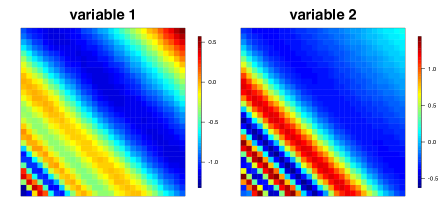
Figure 6: Visualization of the simulated nonstationary data.

To evaluate the performance of the different models on the non-stationary data we have taken $10$ random samples of size $800$ for training and computed the RMSPE on the left out data.

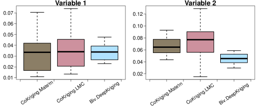
Figure 7: Boxplot of RMSPE for the three different models CoKriging.Matérn, CoKriging.LMC and Biv.DeepKriging with 10-fold cross validation of the nonstationary data.

Figure 7 shows the boxplots of the RMSPE’s for each variable. Biv.DeepKriging performed better than the other predictions for variable 2 whereas for variable 1 the estimates have smaller standard error (Table 1).

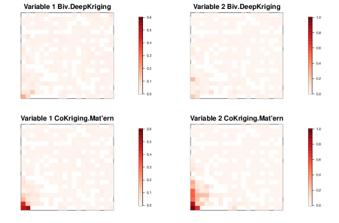
Figure 8: Comparison of absolute deviation of predictions from the truth between Biv.DeepKriging and CoKriging.Matérn. We computed these deviations for the test locations for both the variables.

From Figure 6 we see that the dataset is rough on the lower left region whereas it is comparatively smooth at the top which depicts we can not model the data with the same model structure over the whole region. The CoKriging Model structure does not take into account this nonstationarity within spatial regions. On the other hand bivariate DeepKriging is adaptive towards this spatial nonstationarity hence emarging as a more flexible modelling option. To compare and understand more about our assertion we have computed the absolute error deviation for each test location separately and compared them with the CoKriging.Matérn model which is the second best performing model after Biv.DeepKriging. In Figure 8 we can see that the absolute error is very small for both models over the smoother surface however towards the lower left the absolute error is much higher for CoKriging.Matérn in comparison to Biv.DeepKriging. This implies that the CoKriging model fails to capture the spatial nonstationarity whereas bivariate DeepKriging can capture that well.

4.2 Prediction intervals

Several studies (Ho et al., 2001; Zhao et al., 2008) have proposed various approaches for quantifying the quality of the prediction interval. We have chosen here two specific measures for comparison of the prediction bands, namely prediction interval coverage probability (PICP) and mean prediction interval width (MPIW). In mathematical notations

$$PICP_{u}=\frac{1}{N}\sum_{j=1}^{N}\mathbf{1}_{Z_{u}(s_{j})\in[L_{u}(s_{j}),U_{u}(s_{j})]},\ MPIW_{u}=\frac{1}{N}\sum_{j=1}^{N}[U_{u}(s_{j})-L_{u}(s_{j})],\ u=1,2$$ (20)

where $(L_{u}(s),U_{u}(s))$ are the lower and upper prediction bounds for variable $u$ at location $\mathbf{s}$ and $n$ is the number test samples.

In this section we evaluate our proposed approach of the prediction interval computation with the parametric prediction intervals obtained from cokriging models. We have computed the prediction interval validation metrics (20) for the comparative models using the same set of simulations as defined in 4.1. In all of the following accessments we have computed the $95\%$ prediction bound for predictions in the test set.

Table 2 shows the results for all the simulation scenarios. It can be seen that for the Gaussian simulations where $\mathbf{CoKriging.Mat\acute{e}rn}_{true}$ is optimal the Biv.DeepKriging model gives comparable performance. For non-Gaussian and non-stationary scenarios clearly the Biv.DeepKriging outperforms the other methods by attaining the $95\%$ prediction with smaller width. Note that here we compared the best two models for each simulation scenario that were obtained from point predictions.

Table 2: Comparison of $PICP$ and $MPIW$ over different simulation settings.

Simulation type	Models	$PICP_{1}$	$PICP_{2}$	$MPIW_{1}$	$MPIW_{2}$
Gaussian	$\textbf{CoKriging.Mat\'{e}rn}_{true}$ Biv.DeepKriging	0.958 0.969	0.952 0.966	0.303 0.439	0.276 0.388
non-Gaussian	CoKriging.LMC Biv.DeepKriging	0.990 0.987	0.975 0.988	2.173 1.753	16.79 7.534
non-stationary	CoKriging.Matérn Biv.DeepKriging	0.955 0.975	0.968 0.973	0.421 0.192	0.175 0.125

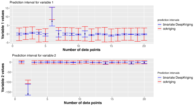
Figure 9: Prediction interval for variable 1 and variable 2 for the non-Gaussian simulation. Here the red interval indicates the prediction interval generated by CoKriging.LMC and the blue interval is for Biv.DeepKriging.

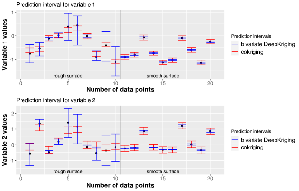
Figure 10: Prediction interval for variable 1 and variable 2 for the nonstationary simulation. Here the red interval signifies the prediction interval generated by CoKriging.Matérn and the blue interval is for Biv.DeepKriging.

Although in Section 4.1 we have shown how the nolinearity in Biv.DeepKriging help to capture the nonstationarity in the data, it is also important to show how the proposed Biv.DeepKriging model improves prediction intervals. To investigate this we chose some points from the test set randomly and computed the prediction intervals based on Biv.DeepKriging and cokriging.

Figure 9 and 10 show the prediction intervals for the Biv.DeepKriging and the cokriging models for non-Gaussian and nonstationary simulations. The prediction intervals for Biv.DeepKriging are adaptive over space. Biv.DeepKriging provides large prediction bounds for extreme observations and also for regions which have higher variance while for regions which are non-extreme and contains low variability it gives smaller prediction bounds.

4.3 Computation time

Based on the same simulation setting we investigate the computational time of Biv.DeepKri- ging compared to CoKriging.Matérn with different number of observations N. We have fully optimized the model and have measured the computation time for the whole process in each case. We have also compared CoKriging.Matérn with both of our proposed methods for point prediction as well as interval prediction.

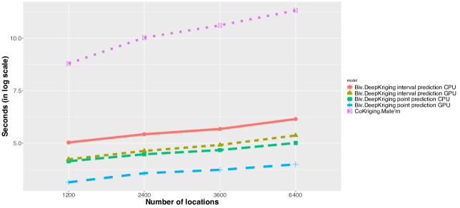
Figure 11: Total computation time (in secconds) for different models in log scale for different number of locations

Figure 11 shows the comparison results. As it can be seen Biv.DeepKriging always outperforms CoKriging.Matérn in computational time hence it is much more scalable when the sample size increases. For example, when N = 6400, which is the largest sample size we have considered, it takes more than 23 hours (83,484 seconds) to train the cokriging model, which makes it computational infeasible for larger N. However, for the same data size, Biv.DeepKriging with prediction interval only costs 7.85 minutes (471 seconds) without GPU acceleration and 3.58 minutes (215 seconds) with a Tesla P100 GPU. We used the GPU from Ibex a shared computing platform at KAUST. For a more powerful GPU, the computational cost will be further reduced.

5 Application

We have fitted Biv.DeepKriging on the wind data discussed in Section 2. We have used 3 layers of basis functions with $K=100,361,1369$ respectively. The neural network consists of $L=7$ layers with $M_{1}=M_{2}=M_{3}=M_{4}=100$ for first 4 layers, $M_{5}=50,M_{6}=50$ and $M_{7}=2$ nodes in the final layer. By using a sample from a uniform distribution, the model weights were initialized, and a learning rate of 0.01 was selected. The dataset consists of 506,771 locations. However, due to computational issues, the cokriging models could only handle a small subsample of the data. For this reason, we have randomly chosen $147,000$ locations for training of the cokriging model. On the other hand, the Biv.DeepKriging can easily handle the full data. Hence we have fitted two different sets of models with deep neural networks, first with $147,000$ ($\textbf{Biv.DeepKriging}_{147000}$) and second with $450,000$ ($\textbf{Biv.DeepKriging}_{450000}$) locations and we randomly chosen $1000$ locations from the rest for testing. To make the cokriging model more competitive and to reduce the computational burden, we have splitted the data into 100 sub-regions and fitted the model on each sub-region independently.

Table 3 shows that Biv.DeepKriging outperforms $\mathbf{CoKriging.Mat\acute{e}rn}$ in RMSPE.

Table 3: RMSPE for $\mathbf{CoKriging.Mat\acute{e}rn}$ and Biv.DeepKriging.

Models	$\mathbf{RMSPE}_{1}$	$\mathbf{RMSPE}_{2}$
$\mathbf{CoKriging.Mat\acute{e}rn}$	0.882	4.066
$\textbf{Biv.DeepKriging}_{147000}$	0.488	0.438
$\textbf{Biv.DeepKriging}_{450000}$	0.394	0.392

Next we look at the 95% prediction intervals provided by Biv.DeepKriging and CoKriging.Matérn. From Table 4 we can see that even though the MPIW for CoKriging I is smaller than Biv.DeepKriging, it fails drastically containing the true values within its bounds.

Table 4: PICP and MPIW with $\mathbf{CoKriging.Mat\acute{e}rn}$ and Biv.DeepKriging for variable 1 and variable 2 respectively.

Models	$PICP_{1}$	$PICP_{2}$	$MPIW_{1}$	$MPIW_{2}$
$\mathbf{CoKriging.Mat\acute{e}rn}$	0.601	0.734	1.671	1.343
Biv.DeepKriging	0.971	0.950	1.226	1.340

We have also captured the total computation time using Biv.DeepKriging and CoKriging I. For CoKriging I total computation time was 2.18 days (188,352 seconds) where as for Biv.DeepKriging it took 16.81 minutes (1009 seconds) for point prediction and 55.61 minutes (3337 seconds) for interval prediction.

5.1 Spatial interpolation of wind field data

We have given a high resolution interpolation (from $5km\times 5km$ to $1km\times 1km$) for the region near NEOM, an upcoming smart city in Saudi Arabia. This downscaling can improve our understanding of the wind patterns. Sanchez Gomez and Lundquist (2020) have explored how the change in wind direction affect wind turbine performance.

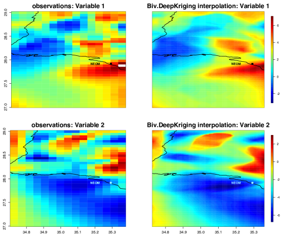
Figure 12: Spatial downscaling from resolution of $5km\times 5km$ to $1km\times 1km$ of the U and V component of wind over the region NEOM

Hence understanding the exact wind patterns in a high resolution field will help in wind energy setup in the area. Figure 12 gives a visual representation of the spatial interpolation carried out using Biv.DeepKriging.

6 Discussion

In this work, we have extended the univariate DeepKriging to bivariate scenario for spatial prediction without any parametric assumption of the underlying distribution of the data. We have also introduced a nonparametric approach for prediction interval computation for this deep learning based spatial modelling architecture. Our model is generally compatible with non-stationarity, non-linear relationships, and non-Gaussian data.

In our implementation we have chosen radial basis functions for spatial embedding. However for long range spatial dependence and circular covariance structures choice of other basis functions such as smoothing spline basis functions (Wahba, 1990), wavelet basis functions (Vidakovic, 2009) can be explored.

The loss function used to Biv.DeepKriging is a weighted MSE where weights are proportional to the variance of the variables. More complex weights can be incorporated to capture complex terrain behaviours. In our study we have not considered topographical elevation. This can be in incorporated by using relevant covariates or by creating an adaptve loss function.

An interesting avenue of future work for prediction intervals is to extend the conformal prediction methods of Mao et al. (2020) to the deepKriging case. This method is model free and thus would avoid the assumption that the prediction intervals are a symmetric t distribution.

Biv.DeepKriging can be suitable for any large-scale environmental application where high resolution spatial interpolation is a requirement.

References

- Adler (2010) Adler, R. J. (2010). The geometry of random fields. SIAM.
- Agarwal et al. (2021) Agarwal, G., Y. Sun, and H. J. Wang (2021). Copula-based multiple indicator kriging for non-Gaussian random fields. Spatial Statistics 44, 100524.
- Apanasovich et al. (2012) Apanasovich, T. V., M. G. Genton, and Y. Sun (2012). A valid Matérn class of cross-covariance functions for multivariate random fields with any number of components. Journal of the American Statistical Association 107(497), 180–193.
- Arain et al. (2007) Arain, M., R. Blair, N. Finkelstein, J. Brook, T. Sahsuvaroglu, B. Beckerman, L. Zhang, and M. Jerrett (2007). The use of wind fields in a land use regression model to predict air pollution concentrations for health exposure studies. Atmospheric Environment 41(16), 3453–3464.
- Ba and Joseph (2012) Ba, S. and V. R. Joseph (2012). Composite Gaussian process models for emulating expensive functions. The Annals of Applied Statistics 6(4), 1838–1860.
- Bardeen et al. (1986) Bardeen, J. M., J. Bond, N. Kaiser, and A. Szalay (1986). The statistics of peaks of Gaussian random fields. The Astrophysical Journal 304, 15–61.
- Bengtsson and Shukla (1988) Bengtsson, L. and J. Shukla (1988). Integration of space and in situ observations to study global climate change. Bulletin of the American Meteorological Society 69(10), 1130–1143.
- Borchani et al. (2015) Borchani, H., G. Varando, C. Bielza, and P. Larranaga (2015). A survey on multi-output regression. Wiley Interdisciplinary Reviews: Data Mining and Knowledge Discovery 5(5), 216–233.
- Boucher et al. (2009) Boucher, M.-A., L. Perreault, and F. Anctil (2009). Tools for the assessment of hydrological ensemble forecasts obtained by neural networks. Journal of Hydroinformatics 11(3-4), 297–307.
- Cannon and Whitfield (2002) Cannon, A. J. and P. H. Whitfield (2002). Downscaling recent streamflow conditions in British Columbia, Canada using ensemble neural network models. Journal of Hydrology 259(1-4), 136–151.
- Changyong et al. (2014) Changyong, F., W. Hongyue, L. Naiji, C. Tian, H. Hua, L. Ying, et al. (2014). Log-transformation and its implications for data analysis. Shanghai archives of psychiatry 26(2), 105.
- Chen et al. (2022) Chen, W., Y. Li, B. J. Reich, and Y. Sun (2022). Deepkriging: Spatially dependent deep neural networks for spatial prediction. Accepted, Statistica Sinica, to appear.
- Cracknell and Reading (2014) Cracknell, M. J. and A. M. Reading (2014). Geological mapping using remote sensing data: A comparison of five machine learning algorithms, their response to variations in the spatial distribution of training data and the use of explicit spatial information. Computers & Geosciences 63, 22–33.
- Cressie (1990) Cressie, N. (1990). The origins of kriging. Mathematical geology 22(3), 239–252.
- Cressie and Huang (1999) Cressie, N. and H.-C. Huang (1999). Classes of nonseparable, spatio-temporal stationary covariance functions. Journal of the American Statistical Association 94(448), 1330–1339.
- Cressie and Johannesson (2008) Cressie, N. and G. Johannesson (2008). Fixed rank kriging for very large spatial data sets. Journal of the Royal Statistical Society: Series B (Statistical Methodology) 70(1), 209–226.
- Cressie (1993) Cressie, N. A. (1993). Statistics for spatial data. Wiley Series in Probability and Statistics. Wiley.
- Daw et al. (2022) Daw, R., M. Simpson, C. K. Wikle, S. H. Holan, and J. R. Bradley (2022). An overview of univariate and multivariate Karhunen Loève Expansions in statistics. Journal of the Indian Society for Probability and Statistics 23, 285–326.
- De Oliveira et al. (2002) De Oliveira, V., K. Fokianos, and B. Kedem (2002). Bayesian transformed Gaussian random field: A Review. Ouyou toukeigaku 31(3), 175–187.
- Fonseca and Steel (2011) Fonseca, T. C. and M. F. Steel (2011). Non-Gaussian spatiotemporal modelling through scale mixing. Biometrika 98(4), 761–774.
- Fuentes (2001) Fuentes, M. (2001). A high frequency kriging approach for nonstationary environmental processes. Environmetrics: The official journal of the International Environmetrics Society 12(5), 469–483.
- Genton and Kleiber (2015) Genton, M. G. and W. Kleiber (2015). Cross-covariance functions for multivariate geostatistics. Statistical Science 30(2), 147–163.
- Goovaerts (1998) Goovaerts, P. (1998). Ordinary cokriging revisited. Mathematical Geology 30(1), 21–42.
- Hastie et al. (2001) Hastie, T., R. Tibshirani, and J. Friedman (2001). The elements of statistical learning. springer series in statistics. In :. Springer.
- Hinton et al. (2012) Hinton, G., N. Srivastava, and K. Swersky (2012). Neural networks for machine learning lecture 6a overview of mini-batch gradient descent. Cited on 14(8), 2.
- Ho et al. (2001) Ho, S. L., M. Xie, L. Tang, K. Xu, and T. Goh (2001). Neural network modeling with confidence bounds: a case study on the solder paste deposition process. IEEE Transactions on Electronics Packaging Manufacturing 24(4), 323–332.
- Jeong and Kim (2005) Jeong, D.-I. and Y.-O. Kim (2005). Rainfall-runoff models using artificial neural networks for ensemble streamflow prediction. Hydrological Processes: An International Journal 19(19), 3819–3835.
- Journal and Alabert (1989) Journal, A. and F. Alabert (1989). Non-Gaussian data expansion in the earth sciences. Terra Nova 1(2), 123–134.
- Kasiviswanathan and Sudheer (2016) Kasiviswanathan, K. and K. Sudheer (2016). Comparison of methods used for quantifying prediction interval in artificial neural network hydrologic models. Modeling Earth Systems and Environment 2(1), 22.
- Khosravi et al. (2011) Khosravi, A., S. Nahavandi, D. Creighton, and A. F. Atiya (2011). Comprehensive review of neural network-based prediction intervals and new advances. IEEE Transactions on neural networks 22(9), 1341–1356.
- Krizhevsky et al. (2012) Krizhevsky, A., I. Sutskever, and G. E. Hinton (2012). Imagenet classification with deep convolutional neural networks. Advances in neural information processing systems 25, 1097–1105.
- LeCun et al. (2015) LeCun, Y., Y. Bengio, and G. Hinton (2015). Deep learning. nature 521(7553), 436–444.
- Li et al. (2019) Li, R., H. D. Bondell, and B. J. Reich (2019). Deep distribution regression.
- Mao et al. (2020) Mao, H., R. Martin, and B. Reich (2020). Valid model-free spatial prediction.
- Millstein et al. (2022) Millstein, D., M. Bolinger, and R. Wiser (2022). What can surface wind observations tell us about interannual variation in wind energy output? Wind Energy 25, 1142–1150.
- Najafabadi et al. (2015) Najafabadi, M. M., F. Villanustre, T. M. Khoshgoftaar, N. Seliya, R. Wald, and E. Muharemagic (2015). Deep learning applications and challenges in big data analytics. Journal of big data 2(1), 1–21.
- Neal (2012) Neal, R. M. (2012). Bayesian learning for neural networks, Volume 118. Springer Science & Business Media.
- Nourani et al. (2021) Nourani, V., N. J. Paknezhad, and H. Tanaka (2021). Prediction interval estimation methods for artificial neural network (ANN)-based modeling of the hydro-climatic processes, a Review. Sustainability 13(4), 1633.
- Nychka et al. (2015) Nychka, D., S. Bandyopadhyay, D. Hammerling, F. Lindgren, and S. Sain (2015). A multiresolution Gaussian process model for the analysis of large spatial datasets. Journal of Computational and Graphical Statistics 24(2), 579–599.
- Nychka et al. (2002) Nychka, D., C. Wikle, and J. A. Royle (2002). Multiresolution models for nonstationary spatial covariance functions. Statistical Modelling 2(4), 315–331.
- Paciorek and Schervish (2003) Paciorek, C. J. and M. J. Schervish (2003). Nonstationary covariance functions for Gaussian process regression. In NIPS, pp. 273–280. Citeseer.
- Posch et al. (2019) Posch, K., J. Steinbrener, and J. Pilz (2019). Variational inference to measure model uncertainty in deep neural networks.
- Reich and Fuentes (2015) Reich, B. J. and M. Fuentes (2015). Spatial bayesian nonparametric methods. In Nonparametric Bayesian Inference in Biostatistics, pp. 347–357. Springer.
- Salvaña et al. (2021) Salvaña, M. L. O., S. Abdulah, H. Huang, H. Ltaief, Y. Sun, M. G. Genton, and D. E. Keyes (2021). High performance multivariate geospatial statistics on manycore systems. IEEE Transactions on Parallel and Distributed Systems 32(11), 2719–2733.
- Sanchez Gomez and Lundquist (2020) Sanchez Gomez, M. and J. K. Lundquist (2020). The effect of wind direction shear on turbine performance in a wind farm in central iowa. Wind Energy Science 5(1), 125–139.
- Schmidt-Hieber (2020) Schmidt-Hieber, J. (2020). Nonparametric regression using deep neural networks with ReLU activation function. The Annals of Statistics 48(4), 1875–1897.
- Srivastav et al. (2007) Srivastav, R., K. Sudheer, and I. Chaubey (2007). A simplified approach to quantifying predictive and parametric uncertainty in artificial neural network hydrologic models. Water Resources Research 43, 10.
- Stein and Corsten (1991) Stein, A. and L. Corsten (1991). Universal kriging and cokriging as a regression procedure. Biometrics 47(2), 575–587.
- Stein (1999) Stein, M. L. (1999). Interpolation of spatial data: some theory for Kriging. Springer Science & Business Media.
- Tong (2010) Tong, W. (2010). Wind power generation and wind turbine design. WIT press.
- Topaloğlu and Pehlivan (2018) Topaloğlu, F. and H. Pehlivan (2018). Analysis of wind data, calculation of energy yield potential, and micrositing application with wasp. Advances in Meteorology 2018, 1687–9309.
- Vidakovic (2009) Vidakovic, B. (2009). Statistical modeling by wavelets, Volume 503. John Wiley & Sons.
- Wahba (1990) Wahba, G. (1990). Spline models for observational data. SIAM.
- Wang et al. (2019) Wang, H., Y. Guan, and B. Reich (2019). Nearest-neighbor neural networks for geostatistics. In 2019 international conference on data mining workshops (ICDMW), pp. 196–205. IEEE.
- Wang et al. (2020) Wang, Y., D. Wang, J. Zhao, and C. Zhu (2020). Wind speed spatial estimation using geostatistical kriging. In IOP Conference Series: Earth and Environmental Science, Volume 619, pp. 012049. IOP Publishing.
- Wikle and Zammit-Mangion (2022) Wikle, C. K. and A. Zammit-Mangion (2022). Statistical deep learning for spatial and spatio-temporal data.
- Xiong et al. (2007) Xiong, Y., W. Chen, D. Apley, and X. Ding (2007). A non-stationary covariance-based kriging method for metamodelling in engineering design. International Journal for Numerical Methods in Engineering 71(6), 733–756.
- Xu and Genton (2017) Xu, G. and M. G. Genton (2017). Tukey g-and-h random fields. Journal of the American Statistical Association 112(519), 1236–1249.
- Yip (2018) Yip, C. M. A. (2018). Statistical characteristics and mapping of near-surface and elevated wind resources in the Middle East. Ph. D. thesis, KAUST.
- Zammit-Mangion et al. (2021) Zammit-Mangion, A., T. L. J. Ng, Q. Vu, and M. Filippone (2021). Deep compositional spatial models. Journal of the American Statistical Association (0162-1459), 1–22.
- Zhang and El-Shaarawi (2010) Zhang, H. and A. El-Shaarawi (2010). On spatial skew-Gaussian processes and applications. Environmetrics: The official journal of the International Environmetrics Society 21(1), 33–47.
- Zhao et al. (2008) Zhao, J. H., Z. Y. Dong, Z. Xu, and K. P. Wong (2008). A statistical approach for interval forecasting of the electricity price. IEEE Transactions on Power Systems 23(2), 267–276.