Automated Polynomial Filter Learning
for Graph Neural Networks

Abstract.

Polynomial graph filters have been widely used as guiding principles in the design of Graph Neural Networks (GNNs). Recently, the adaptive learning of the polynomial graph filters has demonstrated promising performance for modeling graph signals on both homophilic and heterophilic graphs, owning to their flexibility and expressiveness. In this work, we conduct a novel preliminary study to explore the potential and limitations of polynomial graph filter learning approaches, revealing a severe overfitting issue. To improve the effectiveness of polynomial graph filters, we propose Auto-Polynomial, a novel and general automated polynomial graph filter learning framework that efficiently learns better filters capable of adapting to various complex graph signals. Comprehensive experiments and ablation studies demonstrate significant and consistent performance improvements on both homophilic and heterophilic graphs across multiple learning settings considering various labeling ratios, which unleashes the potential of polynomial filter learning.

1. Introduction

In recent years, Graph neural networks (GNNs) have received great attention due to their strong prediction performance in various graph learning tasks, such as node classification (Oono and Suzuki, 2019), link prediction (Zhang and Chen, 2018) and graph classification (Errica et al., 2019). They have been successfully applied to numerous real-world problems since the structured data in many real-world scenarios, such as social networks (Wu et al., 2020), recommendation systems (Wu et al., 2022) and traffic networks (Jiang and Luo, 2022), can be ubiquitously represented as graphs. GNNs’ superiority is due to their capability in capturing and incorporating both node feature and graph structure information through message passing or feature aggregation operations that can be inspired from either spatial domain or spectral domain (Hamilton, 2020; Ma and Tang, 2020).

While numerous GNN architecture designs exist, recent studies suggest that many popular GNNs can be understood as operating various polynomial graph spectral filtering on the graph signal (Defferrard et al., 2016; Kipf and Welling, 2016; Chien et al., 2021; Levie et al., 2018; Xu et al., 2018; Bianchi et al., 2021). From the polynomial graph filter point of view, these GNNs can be broadly categorized into two classes, depending on whether the polynomial graph filters can be either manually designed (e.g., GCN(Kipf and Welling, 2016), APPNP (Klicpera et al., 2019), SGC (Wu et al., 2019a), GNN-LF/HF (Zhu et al., 2021b)) or learned from graph data (e.g., ChebNet (Defferrard et al., 2016), GPRGNN (Chien et al., 2021), BernNet (He et al., 2021)). For instance, GCN adopts a simplified first-order Chebyshev polynomial, and APPNP uses Personalized PageRank to design the graph filter. On the contrary, ChebNet, GPRGNN, and BernNet choose to approximate the graph filter with various polynomials using the Chebyshev basis, Monomial basis, and Bernstein basis respectively whose polynomial coefficients are trainable parameters that can be learned from data.

A large body of literature has demonstrated that in practice, manually designed graph filters perform pretty well on homophilic graphs where nodes with similar features or class labels tend to be connected with each other (Kipf and Welling, 2016; Wu et al., 2019b; Klicpera et al., 2019; Hu et al., 2020). In these cases, simple low-frequency filters, such as those filters in GCN (Kipf and Welling, 2016), SGC (Wu et al., 2019b), and APPNP (Klicpera et al., 2019), typically model the homophilic graph signal well since the graph signal is supposed to be smooth over the edges of the graph. However, it is much more challenging to model the graph signal for heterophilic graphs where the graph signal is not necessarily smooth and highly dissimilar nodes tend to form many edges (Ma et al., 2022; Zhu et al., 2020a, 2021a). For example, in dating networks, people with opposite gender tend to contact each other (Zhao et al., 2013), and different types of amino acids are more likely to link together to form protein structures (Zhu et al., 2020a), etc. Therefore, the low-pass filter via a simple neighborhood aggregation mechanism in GNNs is problematic and not well-suited for heterophilic graphs. In fact, the proper prior knowledge of the heterophilic graph signal is generally unknown. In these cases, learnable polynomial graph filters, such as those in ChebNet, GPRGNN, and BernNet, exhibit some encouraging performance on many heterophilic datasets since they are able to customize graph filters for graphs in order to accommodate their respective assumptions and adapt to various types of graphs by learning the coefficients of polynomial filters. This indicates the profound potential of graph polynomial filter learning.

While GNNs with polynomial graph filter learning are promising due to their great flexibility and powerful expressive capacity, we discover that they still face various limitations through our preliminary study in Section 2. First, we reveal that the learning of polynomial filters is quite sensitive to the initialization of polynomial filters, which leads to unstable performance and a significantly large variance. Second, we find that they sometimes can exhibit poor performance in practice, especially under semi-supervised settings. Third, their performance often underperforms simple graph-agnostic multi-layer perceptrons (MLPs) on heterophilic graphs, which indicates the failure in graph signal modeling. However, the reasons behind these failures are still obscure.

In this work, we aim to explore the potential and limitations of the widely used polynomial graph filter learning technique for modeling complex graph signals in GNNs. Our contribution to be summarized as the following:

• We conduct a novel investigation to study whether existing approaches have fully realized the potential of graph polynomial filter learning. Surprisingly, we discover that graph polynomial filter learning suffers from a severe overfitting problem, which provides a potential explanation for its failures.

• To overcome the overfitting issue, we propose Auto-Polynomial, a novel and general automated polynomial filter learning framework to enhance the performance and generalization of polynomial graph spectral filters in GNNs.

• Comprehensive experiments and ablation studies demonstrate significant and consistent performance improvements on both homophilic and heterophilic graphs across multiple learning settings, which efficiently unleashes the potential of polynomial filter learning.

2. Preliminary

Notations. An undirected graph can be represented by $\mathcal{G}=(\mathcal{V},\mathcal{E})$ where $\mathcal{V}=\left\{\upsilon_{1},...,\upsilon_{n}\right\}$ is the set of the nodes and $\mathcal{E}=\left\{e_{1},...,e_{m}\right\}$ is the set of the edges. Suppose that the nodes are associated with the node feature matrix ${\mathbf{X}}\in\mathbb{R}^{n\times d}$, where $n$ denotes the number of nodes and $d$ denotes the number of features per node. The graph structure of $\mathcal{G}$ can be represented by the adjacency matrix ${\mathbf{A}}$, and ${\hat{{\mathbf{A}}}}={\mathbf{A}}+{\mathbf{I}}$ denotes the adjacency matrix with added self-loops. Then the symmetrically normalized adjacency matrix and graph Laplacian matrix can be defined as ${\tilde{{\mathbf{A}}}}={\tilde{{\mathbf{D}}}}^{-\frac{1}{2}}{\hat{{\mathbf{A}}}}{\tilde{{\mathbf{D}}}}^{-\frac{1}{2}}$ and ${\tilde{{\mathbf{L}}}}={\mathbf{I}}-{\tilde{{\mathbf{A}}}}=\mathbf{I}-{\hat{{\mathbf{D}}}}^{-\frac{1}{2}}{\hat{{\mathbf{A}}}}{\hat{{\mathbf{D}}}}^{-\frac{1}{2}}$ respectively, where ${\hat{{\mathbf{D}}}}$ is the diagonal degree matrix of ${\hat{{\mathbf{A}}}}$. Next, we will briefly introduce the polynomial graph filter as well as the concepts of homophilic and heterophilic graphs.

2.1. Polynomial Graph Filter

Spectral-based GNNs operate graph convolutions in the spectral domain of the graph Laplacian. Many of these methods utilize polynomial graph spectral filters to achieve this operation. The polynomial graph signal filter can be formulated as follows:

$${\mathbf{Y}}={\mathbf{U}}diag[h(\lambda_{1}),\dots,h(\lambda_{n})]{\mathbf{U}}^{\top}{\mathbf{X}}={\mathbf{U}}h(\mathbf{\Lambda}){\mathbf{U}}^{\top}{\mathbf{X}}\approx\sum_{k=1}^{K}\theta_{k}{\tilde{{\mathbf{L}}}}^{k}{\mathbf{X}},$$

where ${\mathbf{X}}\in\mathbb{R}^{n\times d}$ is the input signal and ${\mathbf{Y}}\in\mathbb{R}^{n\times d}$ is the output signal after filtering. ${\tilde{{\mathbf{L}}}}={\mathbf{U}}\mathbf{\Lambda}{\mathbf{U}}^{\top}$ denotes the eigendecomposition of the symmetric normalized Laplacian matrix ${\tilde{{\mathbf{L}}}}$, where ${\mathbf{U}}$ denotes the matrix of eigenvectors and $\mathbf{\Lambda}=diag[\lambda_{1},\dots,\lambda_{n}]$ is the diagonal matrix of eigenvalues. $h(\lambda)$ is an arbitrary filter function that can be approximated by various polynomials $h_{\Theta}(\lambda)=\sum_{k=0}^{K}\theta_{k}\lambda^{k},\lambda\in[0,2]$, where the polynomial coefficients $\Theta=\{\theta_{k}\}_{k=0}^{K}$ determine the shape and properties of the $k$-th order filter.

The filter approximation using polynomials has multiple unique advantages. First, the filtering operation represented by polynomial filters can be equivalently and efficiently computed in the spatial domain using simple recursive feature aggregations, i.e., $\sum_{k=1}^{K}\theta_{k}{\tilde{{\mathbf{L}}}}^{k}{\mathbf{X}}$, without resorting to expensive eigendecomposition that is infeasible for large-scale graphs. Second, the polynomial filters enable localized computations such that it only requires $k$-hop feature aggregation, and only $k$ parameters are needed compared with the non-parametric filter $h(\mathbf{\Lambda})=diag[h(\lambda_{1}),\dots,h(\lambda_{n})]$. Most importantly, the polynomial filter is flexible and general to represent filters with various properties (He et al., 2021) such as low-pass filters, high-pass filters, band-pass filters, band-rejection filters, comb filters, etc. Generally, the polynomial graph filter can be written in the general form:

(1) $${\mathbf{U}}h(\mathbf{\Lambda}){\mathbf{U}}^{\top}{\mathbf{X}}\approx{\mathbf{U}}h_{\Theta}(\mathbf{\Lambda}){\mathbf{U}}^{\top}=\sum_{k=0}^{K}\theta_{k}P_{k}({\mathbf{M}}),$$

where $\{\theta_{k}\}_{k=0}^{K}$ are the polynomial coefficients, $\{P_{k}(x)\}_{k=0}^{K}$ are the polynomial basis, and ${\mathbf{M}}$ is the basic matrix (e.g., normalized graph Laplacian matrix ${\tilde{{\mathbf{L}}}}$ or normalized adjacency matrix ${\tilde{{\mathbf{A}}}}$). Among all the works based on polynomial filters, we will introduce the foundational ChebNet (Kipf and Welling, 2016) and other improved models such as GPRGNN (Chien et al., 2020) and BernNet (He et al., 2021).

ChebNet: Chebyshev polynomials. ChebNet is a foundational work that uses the Chebyshev polynomials to approximate the graph spectral filter:

(2) $$\sum_{k=0}^{K}\theta_{k}T_{k}(\frac{2{\tilde{{\mathbf{L}}}}}{\lambda_{max}}-{\mathbf{I}}),$$

where $\frac{2{\tilde{{\mathbf{L}}}}}{\lambda_{max}}-{\mathbf{I}}$ denotes the rescaled Laplacian matrix, and $\lambda_{max}$ is the largest eigenvalue of ${\tilde{{\mathbf{L}}}}$. The Chebyshev polynomial $T_{k}(x)$ of order $k$ can be computed by the stable recurrence relation $T_{k}(x)=2xT_{k-1}(x)-T_{k-2}(x)$, with $T_{0}(x)=1$ and $T_{k}(x)=x$. The polynomial filter Eq. (2) can be regarded as a special case of the general form in Eq. (1) when we set $P_{k}(x)=T_{k}(x)$ and ${\mathbf{M}}=\frac{2{\tilde{{\mathbf{L}}}}}{\lambda_{max}}-{\mathbf{I}}$.

GPRGNN: Monomial polynomials. GPRGNN approximates spectral graph convolutions by Generalized PageRank (Chien et al., 2021). The spectral polynomial filter of GPRGNN can be represented as follows:

(3) $$\sum_{k=0}^{K}\theta_{k}{\tilde{{\mathbf{A}}}}^{k},$$

which is equivalent to the general form in Eq. (1) when we set $P_{k}(x)=x^{k}$ and ${\mathbf{M}}={\tilde{{\mathbf{A}}}}$.

BernNet: Bernstein polynomials. The principle of BernNet is to approximate any filter on the normalized Laplacian spectrum of a graph using K-order Bernstein polynomials. By learning the coefficients of the Bernstein Basis, it can adapt to different signals and get various spectral filters. The spectral filter of BernNet can be formulated as:

(4) $$\sum_{k=0}^{K}\theta_{k}\frac{1}{2^{K}}\left(\begin{array}[]{l}K\\ k\end{array}\right)(2{\mathbf{I}}-{\tilde{{\mathbf{L}}}})^{K-k}{\tilde{{\mathbf{L}}}}^{k},$$

which is equivalent to the general form in Eq. (1) when we set $P_{k}(x)=\frac{1}{2^{K}}\left(\begin{array}[]{l}K\\ k\end{array}\right)(2-x)^{K-k}x^{k}$ and ${\mathbf{M}}={\tilde{{\mathbf{L}}}}$.

In the aforementioned GNNs, the coefficients, i.e., $\Theta$, determining the polynomial filters are treated as learnable parameters together with other model parameters that are learned by gradient descent algorithms based on the training loss. They have shown encouraging performance on both homophilic and heterophilic graphs since the filter can be adapted to model various types of graph signals whose proper assumptions are generally complex and unknown.

2.2. Homophily and Heterophily

Graphs can be classified into homophilic graphs and heterophilic graphs based on the concept of node homophily (Zhu et al., 2020a; Pei et al., 2020; Ma et al., 2022). In homophilic graphs, nodes with similar features or belonging to the same class tend to connect with each other. For example, in citation networks, papers in the same research field tend to cite each other (Ciotti et al., 2016). In other words, homophilic graphs usually satisfy the smoothness assumption that the graph signal is smooth over the edges. The majority of GNNs are under homophily assumption, and their manually designed low-pass filters filter out the high-frequency graph signal via simple neighborhood aggregation mechanisms that propagate the graph information. For instance, GCN (Kipf and Welling, 2016) uses the first-order Chebyshev polynomial as graph convolution, which is proven to be a fixed low-pass filter (NT and Maehara, 2019). APPNP (Klicpera et al., 2019) uses a Personalized Pagerank(PPR) to set fixed filter coefficients, which has been shown to surpass the high-frequency graph signals (Chien et al., 2021). Generally, these manually designed graph filters exhibit superior performance in various prediction tasks on homophilic graphs.

On the other hand, in heterophilic graphs, nodes with different features or belonging to different classes tend to connect with each other. For example, in dating networks, most users tend to establish connections with individuals of the opposite gender, exhibiting heterophily (Zhu et al., 2021a). In molecular networks, protein structures are more likely to be composed of connections between different types of amino acids (Zhu et al., 2020a). In order to quantify the degree of homophily of the graphs, Pei et al (Pei et al., 2020) have proposed a metric to measure the level of node homophily in graphs:

(5) $$H({\mathcal{G}})=\frac{1}{|\mathcal{V}|}\sum_{v\in\mathcal{V}}\frac{\left|\left\{u\in\mathcal{N}(v):y_{v}=y_{u}\right\}\right|}{|\mathcal{N}(v)|}$$

where $\mathcal{N}(v)$ denotes the neighbour set of node $v$, and $y_{v}$ denotes the label of node $v$. This metric $H({\mathcal{G}})$ measures the average probability that an edge connects two nodes of the same label over all nodes in ${\mathcal{V}}$. When $H({\mathcal{G}})\rightarrow 1$, it indicates the graph is of high homophily since the edge always connects nodes with the same label, while $H({\mathcal{G}})\rightarrow 0$ indicates the graph is of high heterophily where edge always connect nodes with different labels. In fact, the proper prior knowledge of the heterophilic graphs is generally unknown. Therefore, those classic GNNs cannot perform well on heterophilic graphs since their expressive power is limited by fixed filters.

In recent years, many works have been actively exploring GNNs under heterophily. Some examples of heuristic approaches include MixHop (Abu-El-Haija et al., 2019), H2GCN (Zhu et al., 2020b), and GCNII (Chen et al., 2020). For example, MixHop (Abu-El-Haija et al., 2019) is an exemplary method that aggregates messages from higher-order neighbors, thereby enabling the integration of information from different distances. Another notable approach is H2GCN (Zhu et al., 2020b), which aims to address heterophily by separating the ego and neighbor embeddings. GCNII (Chen et al., 2020) adopts various residual connections and more layers to capture distant information in graphs. They all attempt to aggregate information from higher-order neighbors. There also exist multiple approaches inspired by polynomial graph filters (Defferrard et al., 2016; Chien et al., 2021; He et al., 2021). These polynomial graph filter learning approaches have better interpretability than heuristic methods, and they exhibit encouraging performance on some heterophilic graphs, owing to the flexibility and adaptivity to graph signals of various properties. However, there is no consistent performance advantage for either heuristic or graph polynomial filter learning approaches. Both types of methods sometimes underperform graph-agnostic MLPs.

3. Overfitting of graph polynomial filter learning

In this section, we design novel preliminary experiments to investigate the potential and limitations of polynomial graph filter learning in GNNs.

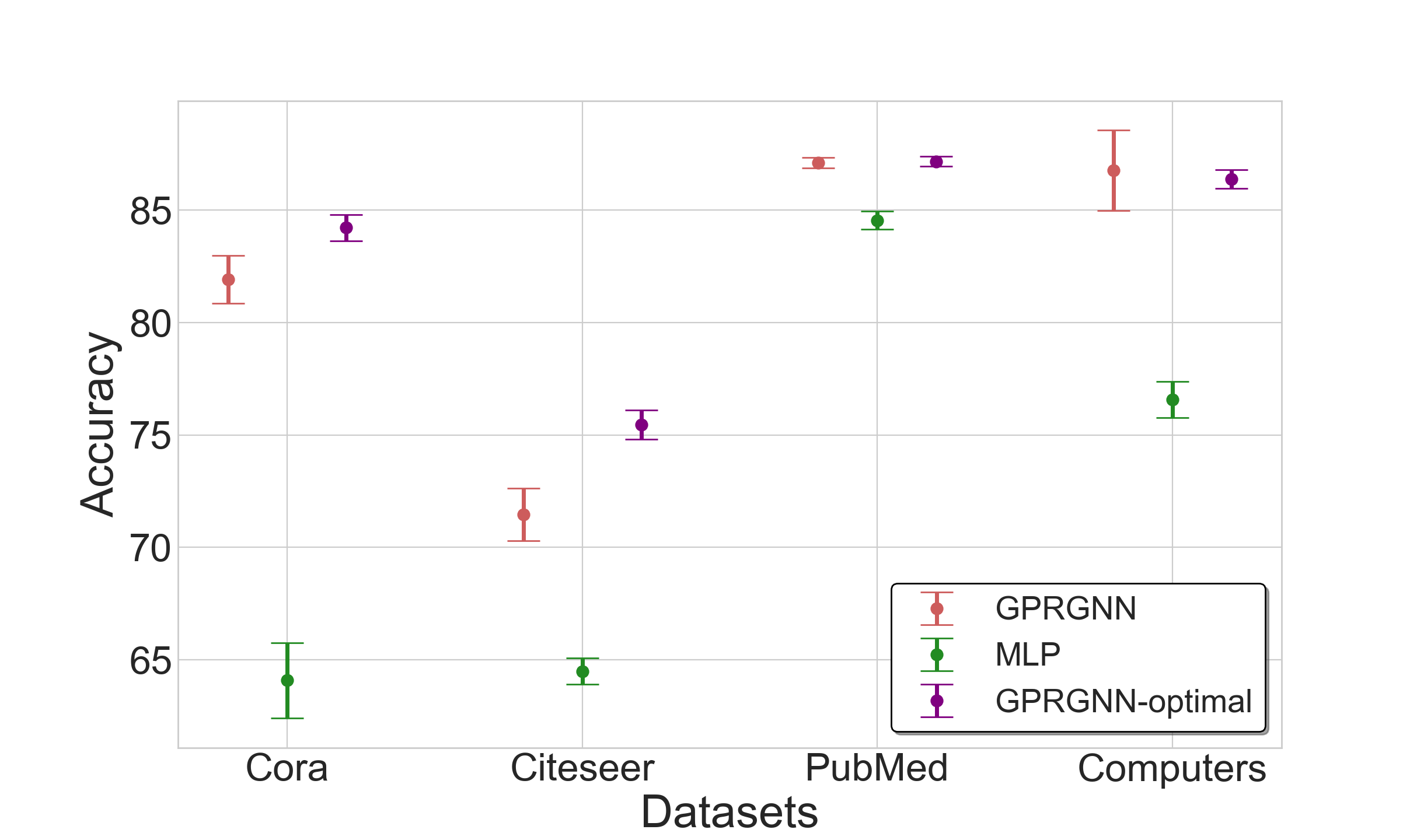
(a) Homophilic datasets.

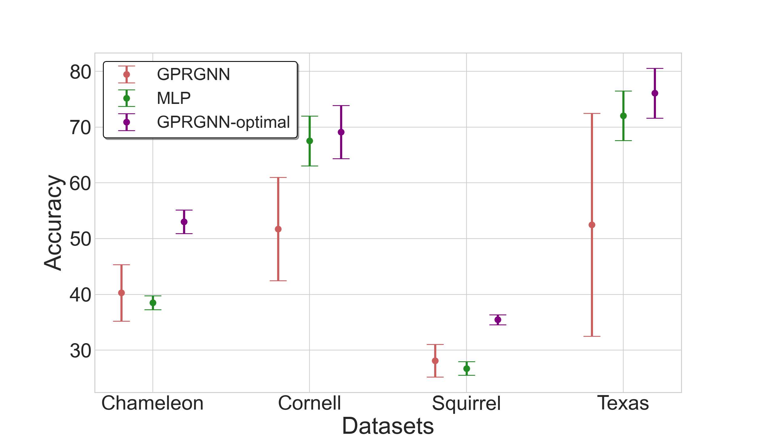
(b) Heterophilic datasets.

Figure 1. The comparison between MLP, GPRGNN, and GPRGNN-optimal on homophilic and heterophilic datasets.

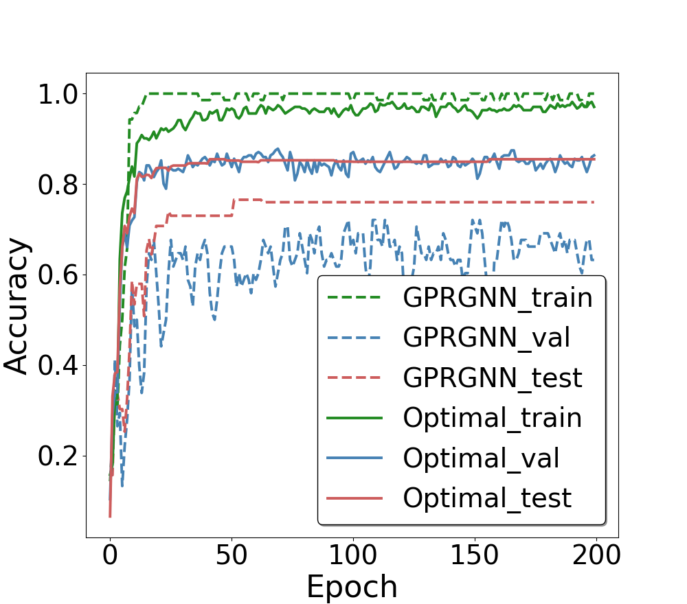
(a) Cora

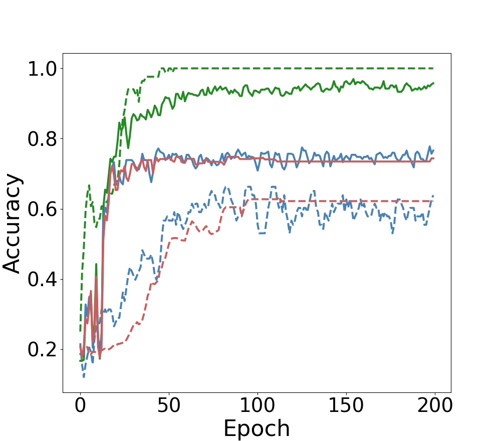
(b) Citeseer

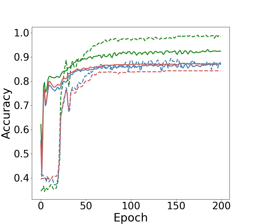
(c) PubMed

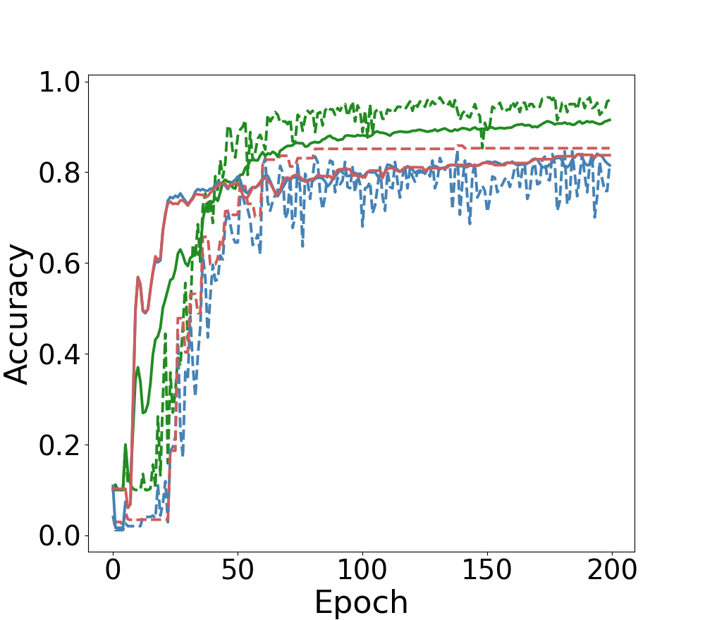
(d) Computers

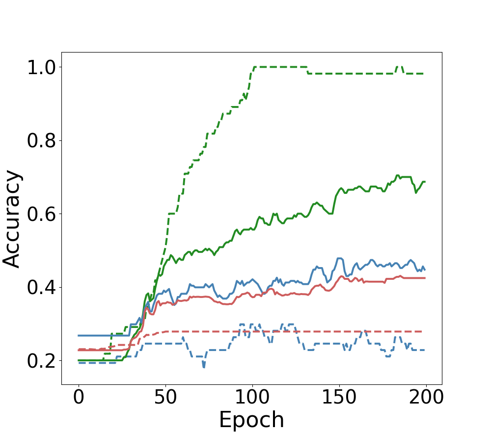
(e) Chameleon

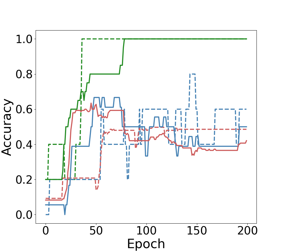
(f) Cornell

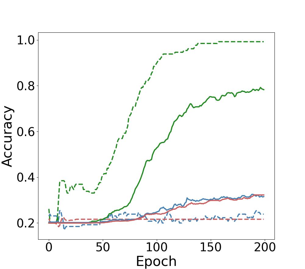
(g) Squirrel

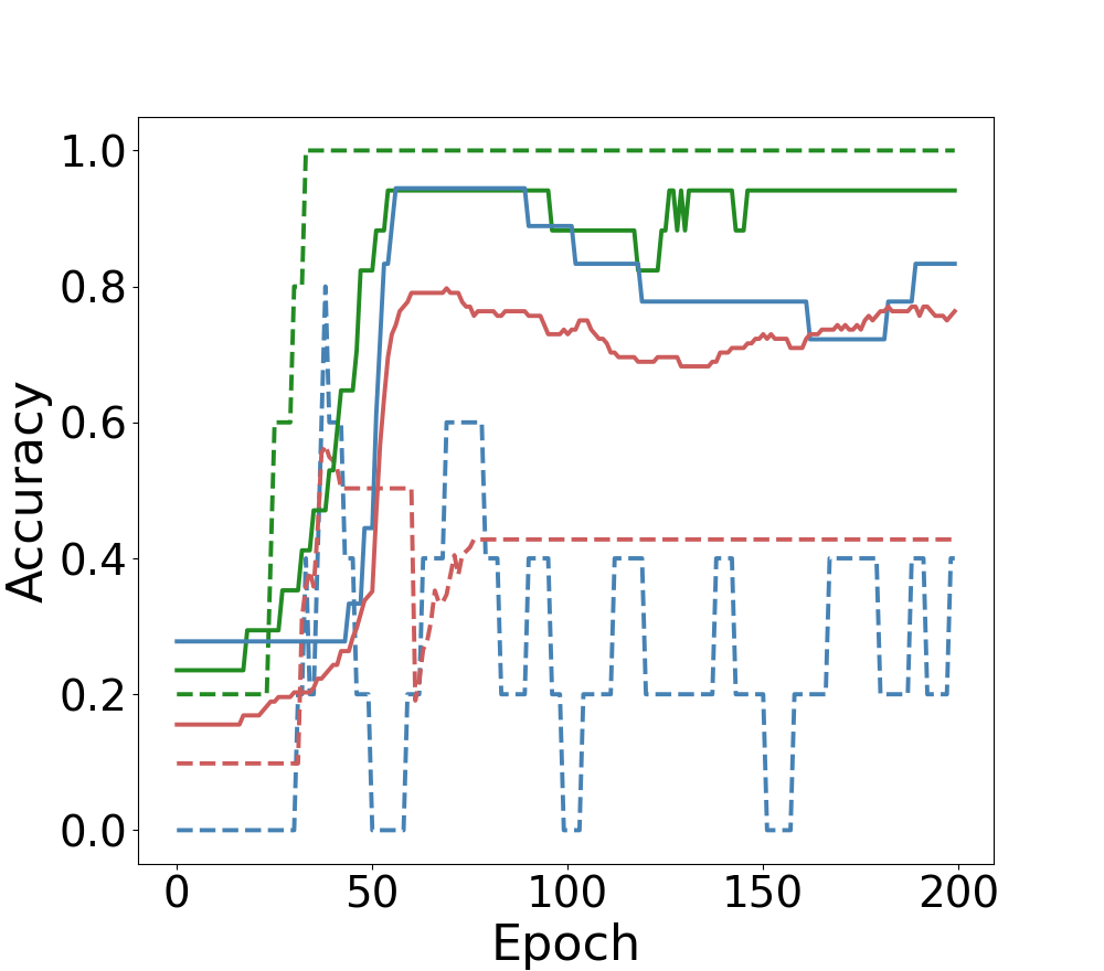
(h) Texas

Figure 2. The training/validation/test accuracy of GPRGNN and GPRGNN-optimal in the training process.

3.1. Search of optimal polynomials

Theoretically speaking, polynomial-based GNNs have strong flexibility, adaptivity, and expressiveness as discussed in Section 2. Although they achieve encouraging performance in some cases, they often fail to show consistent improvement and advantages over simpler designs in practice. On one hand, polynomial-based GNNs do not exhibit notably better performance than manually designed GNNs such as APPNP (Klicpera et al., 2019) and GCNII (Chen et al., 2020) on homophilic datasets even though these manually designed GNNs simply emulate low-pass filters and can be covered and approximated as special cases of polynomial-based GNNs. On the other hand, polynomial-based GNNs (Defferrard et al., 2016; Chien et al., 2021; He et al., 2021) tend to learn inappropriate polynomial weights and often exhibit inferior performance. For example, ChebNet performs noticeably worse than its simplified version, GCN (Kipf and Welling, 2016), which only utilizes the first two Chebyshev polynomials; The improved variants such as GPRGNN (Chien et al., 2021) and BernNet (He et al., 2021) can not consistently outperform heuristically and manually designed alternatives such as H2GCN (Zhu et al., 2020b); and they even underperform graph-agnostic MLPs in some cases.

The failures of polynomial-based GNNs are counterintuitive considering their strong expressively, which then leads to the following critical question: “Have we achieved the full expressiveness and adaptivity of polynomial graph filter learning?” To answer this question, we design a novel experiment to explore the full potential of polynomial filters, i.e., the best performance that the optimal polynomial filter can potentially achieve. Specifically, we choose the monomial polynomial (i.e., $\sum_{k=0}^{K}\theta_{k}{\tilde{{\mathbf{A}}}}^{k}$) as designed in GPRGNN and perform a brute-force search to explore the optimal polynomial filter by a grid search on the polynomial coefficients $\{\theta_{k}\}_{k=0}^{K}$ based on validation accuracy. We denote the GPRGNN with this optimal polynomial filter as GPRGNN-optimal. We compare the performance with the baseline GPRGNN whose polynomial coefficients are learnable parameters guided by training loss.

In detail, we evaluate the performance on semi-supervised node classification tasks on some classic homophilic and heterophilic datasets. In practice, it is computationally expensive to conduct an exhaustive brute-force search on the polynomial coefficients if the polynomial order $K$ is large or the search granularity is fine since the search space will exponentially increase. To reduce the search space for this preliminary study, we set the polynomial order $K=2$ so that we only need to do a grid search over $3$ parameters in the range $\{-0.9,-0.5,-0.2,-0.1,-0.05,0,0.05,0.1,0.2,0.5,0.9\}$. While this coarse search can not cover the whole search space, the results provide performance lower bounds for the optimal polynomial filter. For all models, we adopt the sparse splitting (10% training, 10% validation, and 80% testing) in both homophilic and heterophilic datasets. We tune the hyperparameters such as learning rate and weight decay for GPRGNN following the original paper (Chien et al., 2021). We run the experiments for 10 random data splits and report the mean and standard deviation. The comparison in Figure 1 shows the following observations:

• On homophilic datasets, i.e., Figure 1(a), GPRGNN underperforms GPRGNN-optimal on Cora and CiteSeer, and they achieve comparable performance on PubMed and Computers. Both of them outperform MLP significantly on all datasets. This demonstrates that GPRGNN can learn effective low-pass filters to model the graph signal for homophilic graphs, but it does not fully reach its maximum potential and is notably inferior to the optimal polynomial filter (GPRGNN-optimal) in some cases.

• On heterophilic datasets, i.e., Figure 1(b), GPRGNN exhibits significantly worse performance than GPRGNN-optimal, indicating that GPRGNN learns suboptimal filters. Moreover, GPRGNN does not show notably better performance than MLP, and it even underperforms MLP significantly on Cornell and Texas datasets while GPRGNN-optimal is consistently superior to MLP. This demonstrates that GPRGNN struggles to model the complex graph signal in heterophilic graphs and is far from achieving its theoretical learning potential as indicated by GPRGNN-optimal.

• GPRGNN exhibits unstable performance and high randomness. The learning process of GPRGNN is heavily influenced by the randomness of weights initialization, data splitting and optimization process, leading to a large variance of the final results.

These observations reveal that GNNs based on the polynomial filters indeed have great potential, but the current learning approach is suboptimal, which prevents them from showcasing their optimal capacity. However, the reasons for such failures are unclear.

3.2. Overfitting issue

In this section, we provide further insight into the failures of polynomial filter learning in GNNs and reveal one of the key obstacles to their success. Specifically, we compare the training process of GPRGNN and GPRGNN-optimal by measuring their training, validation, and testing accuracy during the training process. We adopt the same settings in Section 3.1, and only run one split. The training process as shown in Figure 2 provides the following observation:

• GPRGNN always achieves perfect training accuracy close to $100\%$ on all datasets, but its validation performance and test performance are significantly lower. This reveals that the polynomial filter is flexible enough so that the training data can be perfectly fitted but the big generalization gap does not deliver satisfying performance on validation and test data.

• GPRGNN-optimal achieves lower training accuracy than GPRGNN, but its validation and test performance are notably better than GPRGNN. This indicates that GPRGNN suffers from a severe overfitting issue while the optimal polynomial filter can mitigate the overfitting and narrow down this generalization gap.

To summarize, polynomial filter learning in GNNs suffers from a severe overfitting problem that leads to poor generalization. This provides a plausible explanation for the failures of polynomial-based GNNs regardless of their powerful expressiveness.

4. Auto-Polynomial

In this section, we introduce a novel and general automated polynomial filter learning approach to address the aforementioned overfitting issues and improve the effectiveness of graph polynomial filters.

4.1. Automated polynomial filter learning

The polynomial coefficients in polynomial filters serve as key parameters that have a strong influence on the prediction of GNNs. Existing polynomial-based GNNs such as ChebNet, GPRGNN, and BernNet treat the polynomial coefficients the same as other model parameters, both of which are jointly learned through gradient descent algorithms such as Adam (Kingma and Ba, 2014) according to the training loss. Our preliminary study in Section 3 reveals the suboptimal of the widely used polynomial filter learning approach. This suboptimality is partially due to the severe overfitting problem since the filters are adjusted to perfectly fit the labels of training nodes that have a low ratio in the typical semi-supervised learning settings for graph deep learning (Yang et al., 2016; Kipf and Welling, 2016). On the other hand, our brute-force search on the polynomial filter based on the validation accuracy achieves consistently better performance and mitigates the overfitting issues. However, when the polynomial order $K$ is large, it is not plausible to brute-force search the optimal polynomials by trial and error. This motivates us to develop a better automated learning approach for polynomial graph filter learning that mitigates the overfitting.

Auto-Polynomial. We propose Auto-Polynomial, a novel automated polynomial filter learning approach that learns the polynomial coefficients guided by the validation loss inspired by hyperparameter optimization (HPO) and automated machine learning (AutoML). Instead of treating polynomial coefficients the same as other model parameters, we consider these polynomial coefficients as hyperparameters. Let the polynomial coefficients $\Theta=\{\theta_{k}\}_{k=0}^{K}$ represent GNNs with different filtering properties and $w$ denotes other learnable weights in GNNs. The main idea behind Auto-Polynomial is to jointly optimize the coefficients $\Theta$ and the weights $w$ but with totally different targets. Formally, we model the automated polynomial filter learning as a bi-level optimization problem:

(6) $$\underset{\Theta}{\mathrm{min}} \quad\mathcal{L}_{val}(w^{*}(\Theta),\Theta)$$

$$\mathrm{s.t.} \quad w^{*}(\Theta)=\underset{w}{\mathrm{argmin}}(\mathcal{L}_{train}(w,\Theta))$$

where the lower-level optimization problem finds the best model parameters $w^{*}(\Theta)$ based on training loss while the upper-level problem finds the optimal polynomial filter represented by $\Theta$ based on validation loss. Guided by this bi-level optimization problem, the learned GNN model can not only fit the training data accurately but also enhance its performance on validation data, which helps improve generalization ability and alleviate the overfitting problem.

Approximate Computation. The bi-level problem can be solved by alternating the optimization between lower-level and upper-level problems. However, the optimal solution $w^{*}(\Theta)$ in the lower-level problem has a complicated dependency on polynomial coefficients $\Theta$ so that the meta-gradient of upper-level problem, i.e., $\bigtriangledown_{\Theta}\mathcal{L}_{val}(w^{*}(\Theta),\Theta)$, is hard to compute. This complexity becomes even worse when the lower-level problem adopts multiple-step iterations. Therefore, we adopt a simplified and elegant method inspired by DARTS (Liu et al., 2018) to approximate the gradient computation in problem (6):

(7) $$\bigtriangledown_{\Theta}\mathcal{L}_{val}(w^{*}(\Theta),\Theta)\approx\bigtriangledown_{\Theta}\mathcal{L}_{val}(w-\xi\bigtriangledown_{w}\mathcal{L}_{train}(w,\Theta),\Theta)$$

where $\xi$ denotes the learning rate for the lower-level optimization, and only one step gradient is used to approximate the optimal model $w^{*}(\Theta)$. This approximation provides a reasonable solution since $w$ will accumulate the update from all previous training iterations and its initial value $w$ might not be too far away from the optima.

In particular, if we set $\xi=0$, Equation (7) is equivalent to updating $\Theta$ based on the current weights $w$, which is a first-order approximation, a much simpler form of the problem. Although first-order approximation may not provide the best result, it can improve computational efficiency. If we use $\xi>0$, then we can use chain rule to approximate Equation (7):

(8) $$\nabla_{\Theta}\mathcal{L}_{val}\left(w^{\prime},\Theta\right)-\xi\nabla_{\Theta,w}^{2}\mathcal{L}_{train}(w,\Theta)\nabla_{w^{\prime}}\mathcal{L}_{val}\left(w^{\prime},\Theta\right)$$

where $w^{\prime}=w-\xi\nabla_{w}\mathcal{L}_{\text{train }}(w,\Theta)$ denotes the weights after one step gradient descent. In practice, we can apply the finite difference method (Liu et al., 2018) to approximate the second term in Equation (8):

(9) $$\nabla_{\Theta,w}^{2}\mathcal{L}_{\text{train }}(w,\Theta)\nabla_{w^{\prime}}\mathcal{L}_{val}\left(w^{\prime},\Theta\right)$$

$$\approx \frac{\nabla_{\Theta}\mathcal{L}_{train}\left(w^{+},\Theta\right)-\nabla_{\Theta}\mathcal{L}_{train}\left(w^{-},\Theta\right)}{2\varepsilon}$$

where $\varepsilon$ denotes a small scalar in finite difference approximation, $w^{+}=w+\varepsilon\nabla_{w^{\prime}}\mathcal{L}_{val}\left(w^{\prime},\Theta\right)$, and $w^{-}=w-\varepsilon\nabla_{w^{\prime}}\mathcal{L}_{val}\left(w^{\prime},\Theta\right)$. In practice, we also introduce a hyper-parameter $freq$ that specifies the update frequency of polynomial coefficients to further improve the efficiency by skipping this computation from time to time.

4.2. Use cases

The proposed Auto-Polynomial is a general polynomial filter learning framework and it can be applied to various polynomial filter-based GNNs. In this section, we will introduce some representative examples to showcase its application.

Case 1: Auto-GPRGNN. In GPRGNN (Chien et al., 2021), the weights of Generalized PageRank (GPR), i.e., polynomial coefficients $\Theta$ in Equation (3), are trained together with the model parameters $w$. The GPR weights $\Theta$ can be adaptively learned during the training process to control the contribution of the node features and their propagated features in different aggregation layers. GPR provides a flexible way to model various graph signals. However, our preliminary study in Section 3 has shown that GPRGNN can not learn effective filters and faces a serious overfitting problem for the learning of polynomial coefficients. Moreover, its performance is very sensitive to the initialization of filters, data split, and random seeds. The proposed Auto-Polynomial framework can help mitigate these problems. Instead of learning two types of parameters simultaneously, we treat the training of the model parameter $w$ and the GPR weight $\Theta$ as the lower-level and upper-level optimization problems in Equation (6), respectively. In this work, we denote GPRGNN using Auto-Polynomial as Auto-GPRGNN.

Case 2: Auto-BernNet. In BernNet (He et al., 2021), the coefficients of the Bernstein basis $\Theta$ can be learned end-to-end to fit any graph filter in the spectral domain. The training process of BernNet is slightly different from GPRGNN since BernNet specifies an independent learning rate for the polynomial coefficients. To some extent, the learning of polynomial coefficients $\Theta$ is slightly distinguished from the learning of model parameters $w$, which improves the model performance. However, this learning method still has not really brought out the potential of BernNet, and faces the problem of overfitting, especially under semi-supervised learning on heterophilic data. Applying the proposed Auto-Polynomial method to BernNet can ease this problem. We can regard the Bernstein basis coefficients $\Theta$ in BernNet as hyperparameters and optimize them in the Auto-Polynomial bi-level optimization problem. Analogously, we refer to BernNet with Auto-Polynomial as Auto-BernNet.

Input: $\Theta$: coefficients of polynomial filter

$\xi$: learning rate for the lower-level approximation

$\eta_{0}$: learning rate of polynomial filter

$\eta_{1}$: learning rate of model parameters

$w$: model parameters,

$freq$: frequency to update $\Theta$

Output: Graph polynomial filter with coefficients $\Theta$

for $i\leftarrow 1$ to $Iteration$  do

       (Update $\Theta$):

      if i % freq = 0 then

            

            $w^{\prime}_{i}\leftarrow w_{i}-\xi\nabla_{w_{i}}\mathcal{L}_{train}(w_{i},\Theta_{i})$,

            $w^{+}_{i}\leftarrow w_{i}+\varepsilon\nabla_{w^{\prime}_{i}}\mathcal{L}_{val}\left(w^{\prime}_{i},\Theta_{i}\right)$,

            $w^{-}_{i}\leftarrow w_{i}-\varepsilon\nabla_{w^{\prime}_{i}}\mathcal{L}_{val}\left(w^{\prime}_{i},\Theta_{i}\right)$,

            $\nabla_{\Theta_{i},w_{i}}^{2}\mathcal{L}_{train}(w_{i},\Theta_{i})\nabla_{w_{i}^{\prime}}\mathcal{L}_{val}\left(w_{i}^{\prime},\Theta_{i}\right)\leftarrow\text{Equ.}~{}\eqref{eq:2-order}$

            $\nabla_{\Theta_{i}}\mathcal{L}_{val}\left(w^{*}_{i}(\Theta_{i}),\Theta_{i}\right)\leftarrow\text{Equ.}~{}\eqref{eq:chain}$

            $\Theta_{i+1}\leftarrow\Theta_{i}-\eta_{0}\nabla_{\Theta_{i}}\mathcal{L}_{val}(w^{*}_{i},\Theta_{i})$

      else

            $\Theta_{i+1}\leftarrow\Theta_{i}$

       end if

      

      (Update $w$): $w_{i+1}=w_{i}-\eta_{1}\nabla_{w_{i}}\mathcal{L}_{train}(w_{i},\Theta_{i+1})$;

end for

Algorithm 1 Auto-Polynomial Learning Algorithm

4.3. Implementation

In this section, we demonstrate the implementation details of Auto-Polynomial and present the learning procedure in Algorithm 1.

Bi-level update. The whole procedure of Auto-Polynomial includes two main steps: updating the polynomial coefficients $\Theta$ and updating the model parameters $w$. To update $\Theta$, we perform gradient descent with $\nabla_{\Theta}\mathcal{L}_{val}$ to enhance the generalization ability of polynomial filter learning. To reduce memory consumption and increase efficiency, we first employ the finite difference method to compute the second-order term in Equation (9) and then obtain an approximation of $\nabla_{\Theta}\mathcal{L}_{val}$ as Equation (8). In practice, we introduce a hyper-parameter $freq$ to specify the update frequency of polynomial coefficients, so as to further improve the algorithm efficiency in necessary. In other words, $\Theta$ can be updated only once in every $freq$ iterations of model update. To update $w$, we utilize $\nabla_{\Theta}\mathcal{L}_{train}$ to update the model parameters $w$ by fitting the labels of training nodes. Through this alternating update process, we ultimately obtain appropriate polynomial coefficients and model parameters to improve the GNNs’ graph modeling and generalization abilities.

Complexity analysis. The bi-level optimization problem in Auto-Polynomial can be solved efficiently. To be specific, we assume that the computation complexity of the original model is $O(C)$, where $C$ is a known constant. Then the model complexity after applying Auto-Polynomial is $O(\frac{freq+4}{freq}C)$, as we need $4$ extra forward computation when updating $\Theta$. Therefore, the computational complexity of Auto-Polynomial is at most 5 times bigger than the backbone GNN model but it can be effectively reduced by choosing a larger $freq$. In terms of memory cost, Auto-Polynomial does not increase the memory cost significantly no matter how large $freq$ is. The computation time and memory cost will be evaluated in Section 5.

5. Experiment

In this section, we provide comprehensive experiments to validate the effectiveness of Auto-Polynomial under semi-supervised learning and supervised learning settings on both heterophilic and homophilic datasets. Further ablation studies are presented to investigate the influence of training set ratio and update frequency on the model performance.

5.1. Baselines and Datasets

Baselines. We compare the proposed Auto-Polynomial, including use cases Auto-GPRGNN and Auto-BernNet, with 7 baseline models: MLP, GCN (Kipf and Welling, 2016), ChebNet (Defferrard et al., 2016), APPNP (Klicpera et al., 2019), GPRGNN (Chien et al., 2021), BernNet (He et al., 2021) and H2GCN (Zhu et al., 2020a). For GPRGNN and BernNet, we use their the officially released code. For H2GCN, we use the Pytorch version of the original code. For other models, we used the implementation of the Pytorch Geometric Library (Fey and Lenssen, 2019).

Datasets. We conduct experiments on the most commonly used real-world benchmark datasets for node classification. We use 4 homophilic benchmark datasets, including three citation graphs including Cora, Citeseer and PubMed (Sen et al., 2008; Namata et al., 2012), and the Amazon co-purchase graph Computers (McAuley et al., 2015). We also use 4 heterophilic benchmark datasets, including Wikipedia graphs such as Chameleon and Squirrel(Rozemberczki et al., 2021), and webpage graphs such as Texas and Cornell from WebKB. We summarize the dataset statistics in Table 1.

Hyperparameter settings. For APPNP, we set its propagation step size $K=10$ and optimize the teleport probability $\alpha$ over $\left\{0.1,0.2,0.5,0.9\right\}.$ For ChebNet, we set the propagation step $K=2$. For GPRGNN, we set its polynomial order $K=10$. For BernNet, we set the polynomial order $K=10$ and tune the independent learning rate for propagation layer over $\left\{0.002,0.005,0.01,0.05\right\}.$ For H2GCN, we follow the settings in (Zhu et al., 2020b). We search the embedding round $K$ over $\left\{1,2\right\}.$ For all models except H2GCN, we use 2 layer neural networks with 64 hidden units and set the dropout rate 0.5. For Auto-GPRGNN and Auto-BernNet, we use 2-layer MLP with 64 hidden units and set the polynomial order $K=10$. We search the meta learning rate $\eta_{0}$ of Auto-Polynomial over $\left\{0.01,0.05\right\}$ and weight decay over $\left\{0,0.0005\right\}$. We search the learning rate $\xi$ over $\left\{0,0.05\right\}$ and the polynomial weights are randomly initialized. For all models, we adopted an early stopping strategy of 200 epochs with a maximum of 1000 epochs. We use the Adam optimizer to train the models. We optimize learning rate over $\left\{0.002,0.01,0.05\right\}$, and weight decay over $\left\{0,0.0005\right\}$. We select the best performance according to the validation accuracy.

Table 1. Statistics of real-world datasets

Statistics	Cora	Citeseer	Pubmed	Computers	Chameleon	Cornell	Squirrel	Texas
Features	1433	3703	500	767	2325	1703	2089	1703
Nodes	2708	3327	19717	13752	2277	183	5201	183
Edges	5278	4552	44324	245861	31371	277	198353	279
Classes	7	6	5	10	5	5	5	5
$h$	0.83	0.72	0.8	0.8	0.25	0.3	0.22	0.06

5.2. Semi-supervised node classification

Table 2. Semi-supervised learning: mean accuracy ± stdev. The best (second best) results are marked in boldface (underlined).

	MLP	ChebNet	GCN	APPNP	H2GCN	GPRGNN	BernNet	Auto-GPRGNN	Auto-BernNet
Cora	64.79±0.70	81.37±0.93	83.11±1.05	84.71±0.53	82.84±0.69	84.37±0.89	84.27±0.81	84.71±1.19	84.66±0.60
Citeseer	64.90±0.94	71.56±0.86	71.67±1.31	72.70±0.80	72.61±0.67	72.17±0.71	72.08±0.63	72.76±1.18	72.85±0.94
PubMed	84.64±0.41	87.17±0.31	86.40±0.22	86.63±0.36	86.71±0.25	86.42±0.34	86.94±0.18	86.69±0.31	86.81±0.41
Computers	76.80±0.88	86.17±0.58	86.79±0.63	85.76±0.44	84.99±0.54	85.79±1.00	86.84±0.57	86.74±0.61	87.61±0.48
Chameleon	38.61±1.04	49.14±1.66	51.65±1.35	42.13±2.06	50.69±1.60	41.25±4.44	54.11±1.16	55.34±2.93	56.12±1.13
Cornell	66.28±5.97	54.21±5.90	48.83±5.42	63.38±5.28	63.52±6.38	42.83±5.92	63.79±5.30	58.55±7.44	67.03±4.49
Squirrel	26.58±1.37	32.73±0.82	36.98±1.03	29.70±1.31	29.69±0.80	28.83±0.50	26.75±4.49	33.16±2.83	34.48±1.29
Texas	71.62±4.23	70.74±5.10	58.18±5.11	68.45±7.35	75.00±3.42	41.96±12.59	71.62±5.26	73.85±2.64	75.47±3.18

Experimental settings. In semi-supervised learning setting, we randomly split the datasets into training/validation/test sets with the ratio of 10%/10%/80%. We run each experiment 10 times with random splits and report the mean and variance of the accuracy. Note that the data split for semi-supervised learning in the literature is quite inconsistent since existing works usually use different ratios for the homophilic and heterophilic datasets (Chien et al., 2020), or a higher fraction on both the homophilic and heterophilic datasets (Pei et al., 2020; Chen et al., 2020; He et al., 2021). To be fair, we use a consistent ratio for both the homophilic and the heterophilic datasets, which can truly reflect the adaptability of the polynomial filters on different datasets.

Performance analysis. The performance summarized in Table 2 shows the following major observations:

• For homophilic datasets, all GNN models outperform MLP significantly, indicating that the structure information of homophilic graphs can be learned and captured easily. Moreover, Auto-GPRGNN and Auto-BernNet can achieve the best performance in most cases, demonstrating Auto-Polynomial’s superior capability in polynomial graph filter learning.

• For heterophilic datasets, some baselines such as GCN, ChebNet and GPRGNN fail to learn effective polynomial filters and they even underperform graph-agnostic MLP. However, Auto-GPRGNN and Auto-BernNet can outperform all baselines by a significant margin. For instance, Auto-GPRGNN improves over GPRGNN by 14%, 16%, 5%, and 31% on Chameleon, Cornell, Squirrel, and Texas datasets, respectively. Auto-BernNet improves over BernNet by 2%, 4%, 8%, and 4% on Chameleon, Cornell, Squirrel, and Texas datasets, respectively. Moreover, Auto-polynomial effectively reduces the standard deviations in most cases. Especially, Auto-GPRGNN archives a standard deviation 10% lower than GPRGNN on the Texas dataset. These comparisons clearly indicate that Auto-Polynomial is capable of learning polynomial filters more effectively and mitigating the overfitting issue.

5.3. Supervised node classification

Table 3. Supervised learning: mean accuracy ± stdev. The best (second best) results are marked in boldface (underlined).

	MLP	ChebNet	GCN	APPNP	H2GCN	GPRGNN	BernNet	Auto-GPRGNN	Auto-BernNet
Cora	76.20±1.83	86.67±1.99	86.59±1.31	88.70±0.93	87.36± 1.11	88.79±1.37	86.53±1.26	89.05±1.09	88.70±0.93
Citeseer	74.76±1.26	77.44±1.77	77.43±1.42	79.43±1.75	82.78±1.21	78.95±1.93	78.58±1.82	79.76±0.89	79.82±1.55
PubMed	86.51±0.82	88.76±0.58	87.04±0.60	89.10±0.89	87.72±0.46	88.09±0.51	88.25±0.52	89.10±0.54	88.38±0.45
Computers	83.07±0.74	89.11±0.61	87.71±0.73	86.58±0.44	89.04±0.61	87.04±2.71	86.55±0.54	88.56±0.54	88.71±0.71
Chameleon	47.62±1.41	60.68±2.22	61.90±2.19	52.65±2.48	59.58±2.07	62.54±2.77	65.76±1.57	67.38±1.44	68.07±1.48
Cornell	87.03±3.78	77.57±6.05	60.27±11.53	88.65±5.64	87.36±5.82	87.03±4.95	83.24±4.32	91.08±5.28	89.73±3.15
Squirrel	31.16±1.41	40.46±1.81	44.38±1.78	35.86±1.54	35.78±1.31	46.55±1.72	49.30±1.81	47.02±2.54	47.41±1.41
Texas	89.02±2.5	85.88±4.45	73.33±6.09	87.65±1.97	88.24±4.64	81.76±15.8	88.63±3.37	89.41±3.42	90.39±2.83

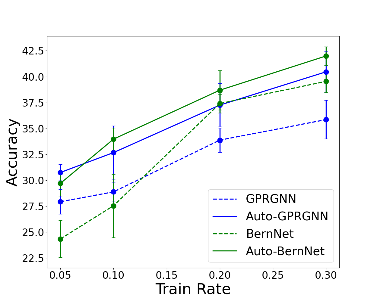
(a) Chameleon

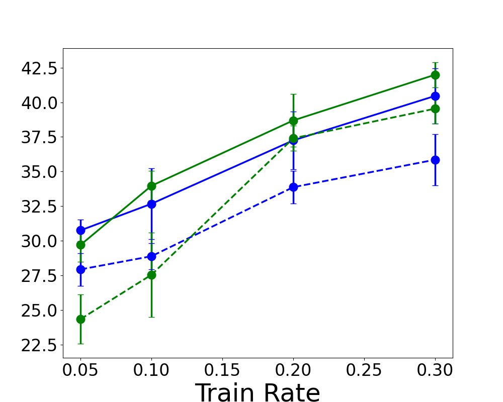
(b) Squirrel

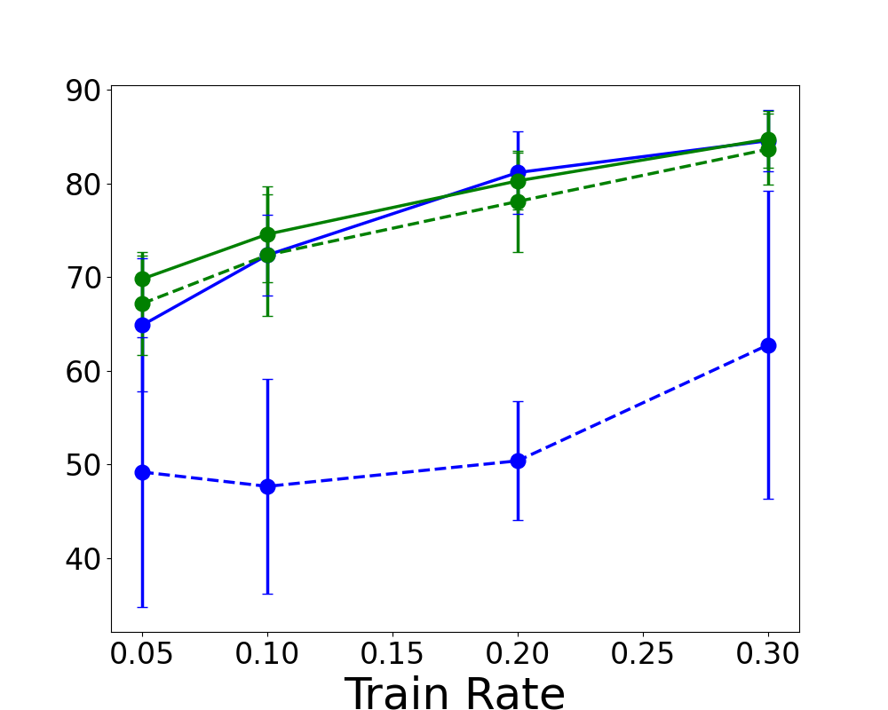
(c) Texas

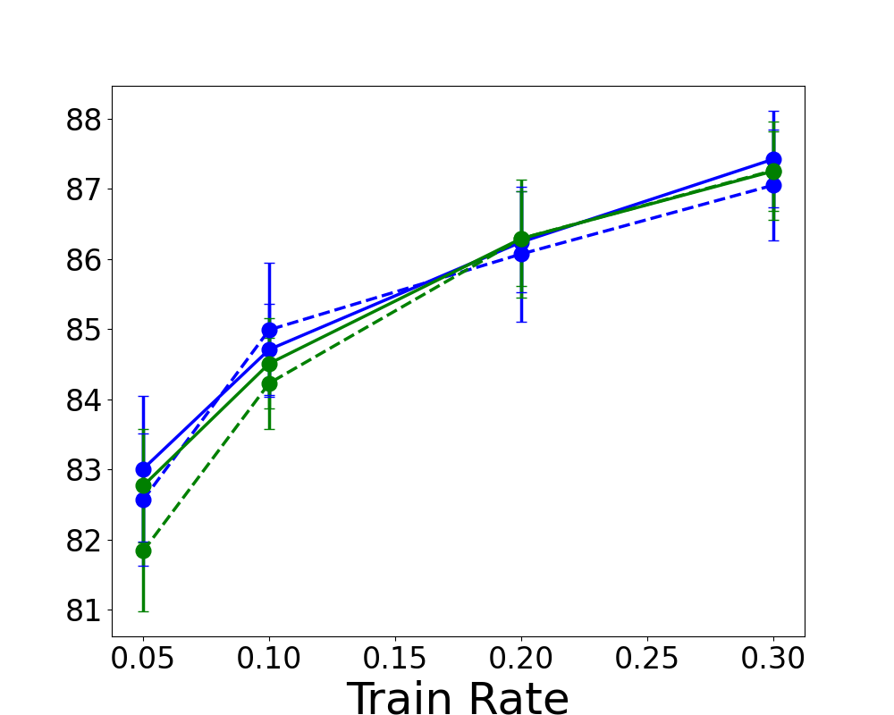
(d) Cora

Figure 3. Results under different ratios on 3 heterophilic datasets and 1 homophilic dataset.

Experimental settings. In supervised learning setting, we randomly split the datasets into training/validation/test sets with the ratio of 48%/32%/32%, following the high ratio in the work (Zhu et al., 2020a). We run each experiment 10 times with random splits and report the mean and variance of the test accuracy.

Performance analysis. The performance summarized in Table 3 shows the following major observations:

• For homophilic datasets, most of the models performed well with small standard deviations, which shows that the existing GNNs are capable of learning proper filters for homophilic graphs. Moreover, Auto-GPRGNN and Auto-BernNet improves their backbone models, GPRGNN and BernNet, indicating that Auto-Polynomial helps them learn better polynomial filters.

• For heterophilic datasets, most of the baselines perform poorly with large standard deviations, which shows that they cannot learn heterophilic graph information well. Models using polynomial filters such as ChebNet, GPRGNN, and BernNet achieve better performance, while Auto-GPRGNN and Auto-BernNet achieve the best or second-best performance in most cases and their standard deviations are smaller in most cases. Especially, Auto-GPRGNN achieves a standard deviation 12% lower than GPRGNN on the Texas dataset. These results indicate the effectiveness of Auto-Polynomial in graph polynomial filter learning.

Table 4. Efficiency of GPRGNN and Auto-GPRGNN on Cora and Chameleon. $freq$ denotes the filter update frequency.

	Cora			Chameleon
Method	Test Acc	Running Time (S)	Memory Cost (MB)	Test Acc	Running Time (S)	Memory Cost (MB)
GPRGNN	84.70±0.47	1.04	49.67	40.03±4.31	1.13	64.43
Auto-GPRGNN ($freq$=1)	84.35±0.47	4.18	66.94	54.96±2.29	5.92	88.29
Auto-GPRGNN ($freq$=2)	84.51±1.03	2.71	66.94	53.71±1.89	3.79	88.29
Auto-GPRGNN ($freq$=3)	84.65±0.73	2.25	66.94	52.71±3.46	3.38	88.29
Auto-GPRGNN ($freq$=4)	84.76±0.96	2.00	66.94	53.23±3.37	2.90	88.29
Auto-GPRGNN ($freq$=5)	83.94±0.79	1.91	66.94	52.91±2.35	2.66	88.29

5.4. Ablabtion study

In this section, we provide ablation studies on the labeling ratio and polynomial update frequency.

Labeling ratio. From the results in semi-supervised and supervised settings in Table 2 and Table 3, it appears that the improvement from Auto-Polynomial is more significant on semi-supervised tasks (low labeling ratio), as compared to supervised tasks (high labeling ratio). This phenomenon motivates the study of how the labeling ratio impacts the effectiveness of our proposed framework. To this end, we fix the validation set ratio at 10%, vary the training set ratio over $\left\{5\%,\ 10\%,\ 20\%,\ 30\%\right\}$, and adjust the test set ratio accordingly. We evaluate the performance on three representative heterophilic datasets (Chameleon, Squirrel and Texas), and one homophilic dataset (Cora). We compare the proposed Auto-GPRGNN and Auto-BernNet with the original GPRGNN and BernNet, following the hyperparameter settings in Section 5.1. The results under different ratios on four datasets are shown in Figure 3, and we can have the following observations:

• Auto-GPRGNN and Auto-BernNet can achieve significant improvements in heterophilic graphs compared to the original GPRGNN and BernNet. This suggests that the Auto-Polynomial framework can help the polynomial filters effectively adapt to heterophilic graphs.

• The improvements of Auto-Polymonial over the backbone models are even more obvious under lower labeling ratios. This shows that when there are not enough labeled samples available, the proposed Auto-Polynomial framework can offer greater advantages in addressing the overfitting issues and enhancing the model’s generalization ability.

Update frequency. In practical implementation, we introduce a hyper-parameter $freq$ to control the update frequency of polynomial coefficients and thus improve the efficiency of our models. To investigate the influence of update frequency on the efficiency and performance of Auto-Polynomial, we vary the frequency at which Auto-GPRGNN updates $\Theta$ and examine the the resulting changes in performance, training time and memory cost. We conduct the experiments on both homophilic dataset (Cora) and heterophilic dataset (Chameleon). The results presented in Table 4 provide the following observations:

• On the homophilic dataset (Cora), reducing the update frequency of Auto-GPRGNN almost does not impact the performance, validating the stability of Auto-Polynomial.

• On the heterohpilic dataset (Chameleon), Auto-GPRGNN outperforms GPRGNN by significantly and is not very sensitive to the update frequency. This indicates that Auto-Polynomial can greatly enhance the model’s efficiency by using an appropriate update frequency, with negligible sacrifice in performance.

• The memory usage of Auto-GPRGNN is approximately 1.3 times that of GPRGNN. However, this increase in memory usage can be deemed acceptable, given the significant improvement achieved by Auto-GPRGNN.

To summarize, Auto-Polynomial provides an effective, stable, and efficient framework to improve the performance and generalization of polynomial filter learning.

6. Related Work

Polynomial Graph Filter. Polynomial graph filters have been widely used as the guiding principles in the design of spectral-based GNNs starting from the early development of ChebNet (Defferrard et al., 2016). It has gained increasing attention recently due to its powerful flexibility and expressiveness in modeling graph signals with complex properties. For instance, some representative works including ChebNet (Defferrard et al., 2016), GPRGNN (Chien et al., 2021) and BernNet (He et al., 2021) utilize Chebyshev basis, Monomial basis, and Bernstein basis, respectively, to approximate the polynomial filters whose coefficients can be learned adaptively to model the graph signal. Therefore, these polynomial-based approaches exhibit encouraging results in graph signal modeling on both homophilic and heterophilic graphs. In this work, we design novel experiments to explore the potential and limitations of graph polynomial learning approaches, and we propose Auto-Polynomial, a general automated learning framework to improve the effectiveness of any polynomial-based GNNs, making this work a complementary effort to existing works.

AutoML on GNNs. Automated machine learning (AutoML) (Hutter et al., 2019) has gained great attention during the past few years due to its great potential in automating various procedures in machine learning, such as data augmentation (Cubuk et al., 2018, 2020), neural architecture searching (NAS) (Zoph and Le, 2016; Liu et al., 2018), and hyper-parameter optimization (HPO) (Franceschi et al., 2018; Feurer and Hutter, 2019; Lorraine et al., 2020). Recent works have applied AutoML to GNN architecture search using various search strategies such as random search (You et al., 2020; Gao et al., 2019, 2021; Tu et al., 2019), reinforcement learning (Gao et al., 2021; Zhou et al., 2019; Lu et al., 2020), evolutionary algorithms (Nunes and Pappa, 2020; Shi et al., 2020; Guan et al., 2021), and differentiable search (Zhao et al., 2020b, 2021, a). However, these works mainly focus on the general architecture search and none of them provides an in-depth investigation into the polynomial filter learning. Moreover, these methods require a vast search space and complex learning algorithms, which can be time-consuming and resource-intensive. Different from existing works, this work provides a dedicated investigation into polynomial graph filter learning and proposes the first automated learning strategy to significantly and consistently improve the effectiveness of polynomial filter learning with a highly efficient learning algorithm.

7. Conclusion

In this work, we conduct a novel investigation into the potential and limitations of the widely used polynomial graph filter learning approach in graph modeling. Our preliminary study reveals the suboptimality and instability of the existing learning approaches, and we further uncover the severe overfitting issues as a plausible explanation for its failures. To address these limitations, we propose Auto-Polynomial, a novel and general automated polynomial graph filter learning framework to improve the effectiveness and generalization of any polynomial-based GNNs, making this work orthogonal and complementary to existing efforts in this research topic. Comprehensive experiments and ablation studies demonstrate the significant and consistent improvements of Auto-Polynomial in various learning settings. This work further unleashes the potential of polynomial graph filter-based graph modeling.

References

- (1)
- Abu-El-Haija et al. (2019) Sami Abu-El-Haija, Bryan Perozzi, Amol Kapoor, Nazanin Alipourfard, Kristina Lerman, Hrayr Harutyunyan, Greg Ver Steeg, and Aram Galstyan. 2019. Mixhop: Higher-order graph convolutional architectures via sparsified neighborhood mixing. In international conference on machine learning. PMLR, 21–29.
- Bianchi et al. (2021) Filippo Maria Bianchi, Daniele Grattarola, Lorenzo Livi, and Cesare Alippi. 2021. Graph neural networks with convolutional arma filters. TPAMI (2021).
- Chen et al. (2020) Ming Chen, Zhewei Wei, Zengfeng Huang, Bolin Ding, and Yaliang Li. 2020. Simple and deep graph convolutional networks. In International conference on machine learning. PMLR, 1725–1735.
- Chien et al. (2020) Eli Chien, Jianhao Peng, Pan Li, and Olgica Milenkovic. 2020. Adaptive universal generalized pagerank graph neural network. arXiv preprint arXiv:2006.07988 (2020).
- Chien et al. (2021) Eli Chien, Jianhao Peng, Pan Li, and Olgica Milenkovic. 2021. Adaptive Universal Generalized PageRank Graph Neural Network. In ICLR.
- Ciotti et al. (2016) Valerio Ciotti, Moreno Bonaventura, Vincenzo Nicosia, Pietro Panzarasa, and Vito Latora. 2016. Homophily and missing links in citation networks. EPJ Data Science 5 (2016), 1–14.
- Cubuk et al. (2018) Ekin D Cubuk, Barret Zoph, Dandelion Mane, Vijay Vasudevan, and Quoc V Le. 2018. Autoaugment: Learning augmentation policies from data. arXiv preprint arXiv:1805.09501 (2018).
- Cubuk et al. (2020) Ekin D. Cubuk, Barret Zoph, Jonathon Shlens, and Quoc V. Le. 2020. Randaugment: Practical Automated Data Augmentation With a Reduced Search Space. In Proceedings of the IEEE/CVF Conference on Computer Vision and Pattern Recognition (CVPR) Workshops.
- Defferrard et al. (2016) Michaël Defferrard, Xavier Bresson, and Pierre Vandergheynst. 2016. Convolutional neural networks on graphs with fast localized spectral filtering. In NeurIPS. 3844–3852.
- Errica et al. (2019) Federico Errica, Marco Podda, Davide Bacciu, and Alessio Micheli. 2019. A fair comparison of graph neural networks for graph classification. arXiv preprint arXiv:1912.09893 (2019).
- Feurer and Hutter (2019) Matthias Feurer and Frank Hutter. 2019. Hyperparameter optimization. Automated machine learning: Methods, systems, challenges (2019), 3–33.
- Fey and Lenssen (2019) Matthias Fey and Jan Eric Lenssen. 2019. Fast graph representation learning with PyTorch Geometric. arXiv preprint arXiv:1903.02428 (2019).
- Franceschi et al. (2018) Luca Franceschi, Paolo Frasconi, Saverio Salzo, Riccardo Grazzi, and Massimiliano Pontil. 2018. Bilevel programming for hyperparameter optimization and meta-learning. In International Conference on Machine Learning. PMLR, 1568–1577.
- Gao et al. (2019) Yang Gao, Hong Yang, Peng Zhang, Chuan Zhou, and Yue Hu. 2019. Graphnas: Graph neural architecture search with reinforcement learning. arXiv preprint arXiv:1904.09981 (2019).
- Gao et al. (2021) Yang Gao, Hong Yang, Peng Zhang, Chuan Zhou, and Yue Hu. 2021. Graph neural architecture search. In International joint conference on artificial intelligence. International Joint Conference on Artificial Intelligence.
- Guan et al. (2021) Chaoyu Guan, Xin Wang, and Wenwu Zhu. 2021. Autoattend: Automated attention representation search. In International conference on machine learning. PMLR, 3864–3874.
- Hamilton (2020) William L. Hamilton. 2020. Graph Representation Learning. Synthesis Lectures on Artificial Intelligence and Machine Learning 14, 3 (2020), 1–159.
- He et al. (2021) Mingguo He, Zhewei Wei, Hongteng Xu, et al. 2021. Bernnet: Learning arbitrary graph spectral filters via bernstein approximation. Advances in Neural Information Processing Systems 34 (2021), 14239–14251.
- Hu et al. (2020) Weihua Hu, Matthias Fey, Marinka Zitnik, Yuxiao Dong, Hongyu Ren, Bowen Liu, Michele Catasta, and Jure Leskovec. 2020. Open graph benchmark: Datasets for machine learning on graphs. Advances in neural information processing systems 33 (2020), 22118–22133.
- Hutter et al. (2019) Frank Hutter, Lars Kotthoff, and Joaquin Vanschoren. 2019. Automated machine learning: methods, systems, challenges. Springer Nature.
- Jiang and Luo (2022) Weiwei Jiang and Jiayun Luo. 2022. Graph neural network for traffic forecasting: A survey. Expert Systems with Applications (2022), 117921.
- Kingma and Ba (2014) Diederik P Kingma and Jimmy Ba. 2014. Adam: A method for stochastic optimization. arXiv preprint arXiv:1412.6980 (2014).
- Kipf and Welling (2016) Thomas N Kipf and Max Welling. 2016. Semi-supervised classification with graph convolutional networks. arXiv preprint arXiv:1609.02907 (2016).
- Klicpera et al. (2019) Johannes Klicpera, Aleksandar Bojchevski, and Stephan Günnemann. 2019. Predict then propagate: Graph neural networks meet personalized pagerank. In ICLR.
- Levie et al. (2018) Ron Levie, Federico Monti, Xavier Bresson, and Michael M Bronstein. 2018. Cayleynets: Graph convolutional neural networks with complex rational spectral filters. Transactions on Signal Processing 67, 1 (2018), 97–109.
- Liu et al. (2018) Hanxiao Liu, Karen Simonyan, and Yiming Yang. 2018. Darts: Differentiable architecture search. arXiv preprint arXiv:1806.09055 (2018).
- Lorraine et al. (2020) Jonathan Lorraine, Paul Vicol, and David Duvenaud. 2020. Optimizing Millions of Hyperparameters by Implicit Differentiation. In Proceedings of the Twenty Third International Conference on Artificial Intelligence and Statistics (Proceedings of Machine Learning Research, Vol. 108), Silvia Chiappa and Roberto Calandra (Eds.). PMLR, 1540–1552. https://proceedings.mlr.press/v108/lorraine20a.html
- Lu et al. (2020) Qing Lu, Weiwen Jiang, Meng Jiang, Jingtong Hu, Sakyasingha Dasgupta, and Yiyu Shi. 2020. Fgnas: Fpga-aware graph neural architecture search. (2020).
- Ma et al. (2022) Yao Ma, Xiaorui Liu, Neil Shah, and Jiliang Tang. 2022. Is Homophily a Necessity for Graph Neural Networks?. In International Conference on Learning Representations. https://openreview.net/forum?id=ucASPPD9GKN
- Ma and Tang (2020) Yao Ma and Jiliang Tang. 2020. Deep Learning on Graphs. Cambridge University Press.
- McAuley et al. (2015) Julian McAuley, Christopher Targett, Qinfeng Shi, and Anton Van Den Hengel. 2015. Image-based recommendations on styles and substitutes. In SIGIR.
- Namata et al. (2012) Galileo Namata, Ben London, Lise Getoor, Bert Huang, and U Edu. 2012. Query-driven active surveying for collective classification. In 10th international workshop on mining and learning with graphs, Vol. 8. 1.
- NT and Maehara (2019) Hoang NT and Takanori Maehara. 2019. Revisiting Graph Neural Networks: All We Have is Low-Pass Filters. arXiv:1905.09550 [stat.ML]
- Nunes and Pappa (2020) Matheus Nunes and Gisele L Pappa. 2020. Neural architecture search in graph neural networks. In Intelligent Systems: 9th Brazilian Conference, BRACIS 2020, Rio Grande, Brazil, October 20–23, 2020, Proceedings, Part I 9. Springer, 302–317.
- Oono and Suzuki (2019) Kenta Oono and Taiji Suzuki. 2019. Graph neural networks exponentially lose expressive power for node classification. arXiv preprint arXiv:1905.10947 (2019).
- Pei et al. (2020) Hongbin Pei, Bingzhe Wei, Kevin Chen-Chuan Chang, Yu Lei, and Bo Yang. 2020. Geom-gcn: Geometric graph convolutional networks. In ICLR.
- Rozemberczki et al. (2021) Benedek Rozemberczki, Carl Allen, and Rik Sarkar. 2021. Multi-scale attributed node embedding. Journal of Complex Networks 9, 2 (2021), cnab014.
- Sen et al. (2008) Prithviraj Sen, Galileo Namata, Mustafa Bilgic, Lise Getoor, Brian Galligher, and Tina Eliassi-Rad. 2008. Collective classification in network data. AI magazine 29, 3 (2008), 93–93.
- Shi et al. (2020) Min Shi, David A Wilson, Xingquan Zhu, Yu Huang, Yuan Zhuang, Jianxun Liu, and Yufei Tang. 2020. Evolutionary architecture search for graph neural networks. arXiv preprint arXiv:2009.10199 (2020).
- Tu et al. (2019) Ke Tu, Jianxin Ma, Peng Cui, Jian Pei, and Wenwu Zhu. 2019. Autone: Hyperparameter optimization for massive network embedding. In Proceedings of the 25th ACM SIGKDD international conference on knowledge discovery & data mining. 216–225.
- Wu et al. (2019a) Felix Wu, Amauri Souza, Tianyi Zhang, Christopher Fifty, Tao Yu, and Kilian Weinberger. 2019a. Simplifying graph convolutional networks. In International conference on machine learning. PMLR, 6861–6871.
- Wu et al. (2019b) Felix Wu, Amauri Souza, Tianyi Zhang, Christopher Fifty, Tao Yu, and Kilian Weinberger. 2019b. Simplifying graph convolutional networks. In ICML.
- Wu et al. (2022) Shiwen Wu, Fei Sun, Wentao Zhang, Xu Xie, and Bin Cui. 2022. Graph neural networks in recommender systems: a survey. Comput. Surveys 55, 5 (2022), 1–37.
- Wu et al. (2020) Yongji Wu, Defu Lian, Yiheng Xu, Le Wu, and Enhong Chen. 2020. Graph convolutional networks with markov random field reasoning for social spammer detection. In Proceedings of the AAAI conference on artificial intelligence, Vol. 34. 1054–1061.
- Xu et al. (2018) Bingbing Xu, Huawei Shen, Qi Cao, Yunqi Qiu, and Xueqi Cheng. 2018. Graph Wavelet Neural Network. In ICLR.
- Yang et al. (2016) Zhilin Yang, William Cohen, and Ruslan Salakhudinov. 2016. Revisiting semi-supervised learning with graph embeddings. In ICML. PMLR, 40–48.
- You et al. (2020) Jiaxuan You, Zhitao Ying, and Jure Leskovec. 2020. Design space for graph neural networks. Advances in Neural Information Processing Systems 33 (2020), 17009–17021.
- Zhang and Chen (2018) Muhan Zhang and Yixin Chen. 2018. Link prediction based on graph neural networks. Advances in neural information processing systems 31 (2018).
- Zhao et al. (2021) Huan Zhao, Lanning Wei, Zhiqiang He, et al. 2021. Efficient graph neural architecture search. (2021).
- Zhao et al. (2013) Kang Zhao, Xi Wang, Mo Yu, and Bo Gao. 2013. User Recommendations in Reciprocal and Bipartite Social Networks–An Online Dating Case Study. IEEE intelligent systems 29, 2 (2013), 27–35.
- Zhao et al. (2020a) Yiren Zhao, Duo Wang, Daniel Bates, Robert Mullins, Mateja Jamnik, and Pietro Lio. 2020a. Learned low precision graph neural networks. arXiv preprint arXiv:2009.09232 (2020).
- Zhao et al. (2020b) Yiren Zhao, Duo Wang, Xitong Gao, Robert Mullins, Pietro Lio, and Mateja Jamnik. 2020b. Probabilistic dual network architecture search on graphs. arXiv preprint arXiv:2003.09676 (2020).
- Zhou et al. (2019) Kaixiong Zhou, Qingquan Song, Xiao Huang, and Xia Hu. 2019. Auto-gnn: Neural architecture search of graph neural networks. arXiv preprint arXiv:1909.03184 (2019).
- Zhu et al. (2021a) Jiong Zhu, Ryan A Rossi, Anup Rao, Tung Mai, Nedim Lipka, Nesreen K Ahmed, and Danai Koutra. 2021a. Graph neural networks with heterophily. In Proceedings of the AAAI Conference on Artificial Intelligence, Vol. 35. 11168–11176.
- Zhu et al. (2020a) Jiong Zhu, Yujun Yan, Lingxiao Zhao, Mark Heimann, Leman Akoglu, and Danai Koutra. 2020a. Beyond homophily in graph neural networks: Current limitations and effective designs. Advances in Neural Information Processing Systems 33 (2020), 7793–7804.
- Zhu et al. (2020b) Jiong Zhu, Yujun Yan, Lingxiao Zhao, Mark Heimann, Leman Akoglu, and Danai Koutra. 2020b. Generalizing graph neural networks beyond homophily. arXiv preprint arXiv:2006.11468 (2020).
- Zhu et al. (2021b) Meiqi Zhu, Xiao Wang, Chuan Shi, Houye Ji, and Peng Cui. 2021b. Interpreting and Unifying Graph Neural Networks with An Optimization Framework. In WWW.
- Zoph and Le (2016) Barret Zoph and Quoc V Le. 2016. Neural architecture search with reinforcement learning. arXiv preprint arXiv:1611.01578 (2016).