Accelerating Distributed ML Training via Selective Synchronization

Abstract

In distributed training, deep neural networks (DNNs) are launched over multiple workers concurrently and aggregate their local updates on each step in bulk-synchronous parallel (BSP) training. However, BSP does not linearly scale-out due to high communication cost of aggregation. To mitigate this overhead, alternatives like Federated Averaging (FedAvg) and Stale-Synchronous Parallel (SSP) either reduce synchronization frequency or eliminate it altogether, usually at the cost of lower final accuracy. In this paper, we present SelSync, a practical, low-overhead method for DNN training that dynamically chooses to incur or avoid communication at each step either by calling the aggregation op or applying local updates based on their significance. We propose various optimizations as part of SelSync to improve convergence in the context of semi-synchronous training. Our system converges to the same or better accuracy than BSP while reducing training time by up to 14$\times$.

I Introduction

DNNs minimize an objective function by iteratively learning the underlying relationships from some training data. Stochastic gradient descent (SGD) [1] is the update rule that enables iterative learning based on the current loss and model parameters. DNNs typically converge after many steps or iterations, and model quality is heavily influenced by certain variables or hyperparameters like batch-size, number of epochs, learning rate, type of optimization (e.g., Nesterov [2], Adam [3], etc.), activation function, weight decay, regularization, etc. Distributed Data-Parallel (DDP) training expedites convergence by launching model replicas over many workers concurrently and periodically synchronize their updates. However, distributed training can suffer from high communication costs due to large model size, large number of workers and available bandwidth. Many techniques attempt to attenuate this slowdown either by reducing the frequency or volume of communication, or relax the constraints on extent of synchronization itself, but speedup is usually achieved at the detriment of final accuracy. We refer to such techniques that implement a loose form of synchronization or apply infrequent communication based on some heuristic as semi-synchronous.

In this paper, we propose SelSync , a semi-synchronous training mechanism that switches between synchronous and local updates by assessing which updates are crucial enough to be communicated and which ones can be applied just locally. It thus achieves accuracy targets akin to BSP, while reducing training time by mitigating expensive communication and applying local updates when possible. We make the following contributions in this work:

• We develop SelSync over the Parameter server (PS) architecture [4] using PyTorch RPC framework [41].

• Implement a low-overhead technique to track changes in gradients on each step and define a threshold metric that correlates gradient changes with the trajectory of model convergence. Based on this threshold, we develop a communication rule that updates a model either locally or synchronously among the participating workers.

• Design a custom data-partitioning scheme optimal for semi-synchronous training mechanisms.

• Show empirically that parameter aggregation performs better than gradient aggregation in semi-synchronous training. This is because local and global model states tend to diverge more in the latter when workers train locally for longer and updates are aggregated infrequently.

• Apply SelSync in non-IID data settings by extending a randomized data-injection approach [39] that significantly improves model accuracy over other federated algorithms.

• We compare SelSync with other state-of-the-art algorithms across a variety of DNNs to validate the efficacy of our approach.

II Background and Related Work

In this section, we introduce some popular and state-of-the-art distributed learning algorithms, and briefly discuss their advantages and limitations. Based on their respective communication patterns, each affects the parallel scaling of distributed training in a distinct manner; we refer to this as the parallel efficiency of DDP training. However, unlike traditional distributed applications, the computational work performed by workers at each training step is not equally important; some updates are more critical than others. This is because the work performed by SGD does not fully compose due to the stochastic nature of gradient descent. We refer to this as the statistical efficiency of distributed training, and describe it in detail in §III-A.

II-A Bulk-Synchronous Parallel (BSP) training

In bulk-synchronous parallel or BSP training, each worker trains a DNN on a unique partition of data sampled in an IID (independent and identically distributed) manner, and aggregate their updates at the end of every training step/iteration. Each step thus involves feeding data to every local model to predict an output, evaluate loss, compute gradients, a communication op to aggregate updates and apply them before proceeding to the next step. DNN training is an iterative-convergent process that makes multiple passes over training dataset (where each pass is an epoch) until loss reaches a low-enough target. A model with parameters $w$ training over $N$ workers in parallel processes mini-batch $\mathit{x_{(i,n)}}$ of size $|\mathit{b}|$ from dataset $\mathcal{B}_{n}$ to minimize loss function $\mathcal{F}$ as:

$$w_{i+1}=w_{i}-\eta\dfrac{1}{N}\sum_{n=1}^{n=N}{\dfrac{1}{|b|}\sum_{\mathit{x_{(i,n)}}\in\mathcal{B}_{n}}\dfrac{\partial}{\partial w_{i}}\mathcal{F}(x_{(i,n)},w_{i})}$$ (1)

Parameters at step $(\mathit{i}+1)$ are updated from parameters at $\mathit{i}$ in a direction opposite to the gradients, and scaled by learning rate (lr) $\eta$. In classic BSP, updates from $N$ workers are reduced at every step. Communication can be performed via central parameter server (PS) [4] or Allreduce-based collectives [42]. The aggregation step in BSP is blocking, i.e., all workers wait for the reduction phase to complete before the next step begins.

Thus, BSP suffers from systems heterogeneity where overall speedup is limited by the slowest worker or straggler [16]. Systems heterogeneity in a cluster arises from workers with different computational capabilities. Assuming negligible IO overhead, total iteration time mainly comprises of the computation and synchronization time: $t_{it}=t_{c}+t_{s}$. The former is the time taken to assess loss and compute gradients, and the latter is time taken to communicate updates among workers. ML accelerators like GPUs and TPUs accelerate computing, making computation overhead negligible (i.e., small $t_{c}$) [5]. Thus, communication or synchronization time ($t_{s}$) tends to be the major bottleneck in scaling-out BSP training.

Due to Amdahl’s law [6], scaling thus does not increase linearly with workers due to high communication cost in DDP. It is possible to overlap computation with communication, but the former tends to be much smaller than the latter and so the scope of parallelizing communication is limited by size of updates to exchange, available bandwidth, inter-node latency, etc. Fig. (1a) shows training throughput (i.e., number of training samples processed per second) relative to a single GPU worker as cluster-size increases with parameter server training. Clusters with size 2 and 4 train with 1 NVIDIA V100 GPU per-node, while clusters of size 8 and 16 train with 2 and 4 GPUs per-node respectively. Inter-node workers communicate over a 5 Gbps interface. For ResNet101 [12], throughput improves by only 3$\times$ even as we scale from 1 to 16 workers. Relative throughput for VGG11 [13] at 2 workers was less than 1.0 due to high communication overhead for the 507 MB model, although it improved later over larger clusters. We thus see that DDP throughput does not increase linearly; throughput does not improve by a factor of $N$ when training is scaled from 1 to $N$ workers.

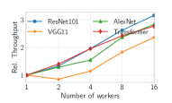
(a) Communication overhead

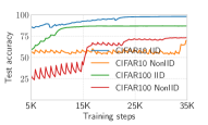
(b) FedAvg: IID vs. non-IID data

Figure 1: (a) Relative throughput from training on NVIDIA V100 GPUs connected over 5Gbps NIC. (b) Training on 10 V100s with 1 label per-worker for non-IID CIFAR10 on ResNet101 and 10 labels per-worker for non-IID CIFAR100 on VGG11.

II-B Federated Averaging (FedAvg)

In federated learning (FL) [7], models are trained over a large number of clients while keeping the data local to each. The data on the clients may have either an IID or non-IID distribution as well. FedAvg [8] is popular FL algorithm for scenarios where workers have limited bandwidth or data privacy concerns. Here, updates from only a fraction of clients are aggregated infrequently at an interval specified by the user. Although FedAvg reduces the communication frequency considerably, it may suffer from high generalization error (i.e., lower test accuracy) due to infrequent synchronization. Thus, there is a complex trade-off space between the communication savings and model quality (i.e., parallel and statistical efficiency) in FedAvg. With its low-frequency, high-volume communication strategy, FedAvg collects updates from fraction $C$ of $N$ workers $x$ times in every epoch, such that synchronization factor $E$=$1/x$. For e.g., $C$=0.5 with $E$=0.25 implies parameters are synchronized among half the devices 4 times (uniformly spaced) over each epoch. One of the key objectives of FL is to improve convergence on workers with non-IID data. This is especially common in mobile/edge computing where data is stored in a decentralized manner across workers. The performance difference from training on balanced vs. unbalanced data with FedAvg is shown in Fig. (1b) from running ResNet101 and VGG11. We train on a cluster of 10 V100 GPUs such that non-IID versions of CIFAR10 (with a total of 10 labels) and CIFAR100 (with 100 labels) [9] are partitioned as 1 and 10 labels per-worker respectively. We set $C$=1 and $E$=0.1 so updates were collected from all workers 10 times in an epoch (every 1/10th epoch).

II-C Stale-Synchronous Parallel (SSP)

SSP [51] is a PS-based approach to mitigate systems heterogeneity between workers which train asynchronously and independently update the global parameters on the central PS in a non-blocking manner. However, the asynchronicity is conditional; synchronization is enforced by blocking faster workers when they exceed the slower workers by a user-specified threshold. Once the threshold exceeds, faster workers are forced to halt and wait for slower workers to catch up. For e.g., setting staleness threshold $s$=100 implies fast workers cannot exceed slow workers by more than 100 iterations. Thus, SSP combines non-blocking execution of asynchronous training while still ensuring the divergence of model parameters between slow and fast workers stays within bounds, determined by $s$. Compared to fully asynchronous training, this reduces staleness effects and inconsistent model states among workers to an extent. In BSP, each of the $N$ workers processes mini-batch size $b$ in a single step. As updates are aggregated at each step, total computational work done in BSP corresponds to its global batch-size $Nb$. Comparatively, SSP performs lesser work per-step as updates computed from a worker over batch-size $b$ are sent asynchronously to the PS. One could theoretically increase worker batch-size to $Nb$ so as to perform the same amount of work as BSP. However, this increases both the computational and resource requirements on a worker, shown in Fig. (2). The computation time across different batch sizes on an NVIDIA K80 is shown in Fig. (2a) for various image and language models Correspondingly, Fig. (2b) shows how memory consumption on a worker shoots up with the batch-size. Transformer [11] on WikiText-103 [17] failed to scale beyond $b$ = 64 due to OOM (out-of-memory) error as memory requirements exceeded the GPU’s 12GB capacity. AlexNet [14] training on the large ImageNet-1K [15] dataset had high memory utilization with large $b$ when using PyTorch’s torchvision.datasets.ImageFolder for data loading and batching [10]. Although relatively smaller in size, ResNet101 is the deepest of all the models evaluated here (with 101 layers). Thus, feeding more samples with larger $b$ increases the forward passes made through the layers of the network which in turn increases computation time on larger batches. If cluster-size $N$ is too large, setting per-worker batch-size to $Nb$ would greatly increase the compute time and memory on each worker, thus making SSP impractical or even prone to failures in those scenarios.

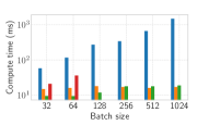
(a) Compute time vs. batch-size

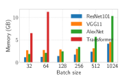
(b) Memory util. vs. batch-size

Figure 2: Setting worker batch-size to $Nb$ in SSP ensures same amount of work is done at each iteration as in BSP. However, computation and memory requirements also increase with batch-size, as measured on a Tesla K80 GPU.

Summary: DDP methods either maximize useful work by iteratively aggregating worker updates (BSP), or speedup training by reducing communication frequency (FedAvg), or loosen the constraints on synchronization itself (SSP). The latter two attain considerable speedup over BSP when they work, but see significant drop in final accuracy/loss when they don’t. This is because they only consider the systems aspect and not the statistical aspect of parallelizing DNN training. We describe in §III-B on how we attempt to bridge this gap by designing a training strategy that considers both.

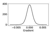
(a) ResNet101 at epoch 1

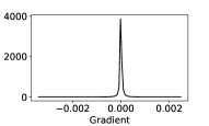
(b) ResNet101 at epoch 50

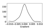
(c) Transformer at epoch 1

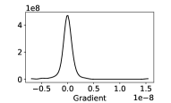
(d) Transformer at epoch 4

Figure 3: Gradient Kernel density estimates (or KDE on the Y-axis) over the epochs for ResNet101 layer layer4_1_conv1_weight and Transformer layer transformer_encoder_layers_0_norm1_weight. Gradients are volatile in the early epochs ((a) and (c)), but get smaller and saturate as gradient variance decreases over the course of training ((b) and (d)).

II-D Other communication-optimizing DDP methods

Gradient compression techniques lower the volume or density of gradient tensors based on some rule or heuristic. They can broadly be classified into: sparsification, quantization or low-rank approximations. We send a subset of gradient values and its corresponding indices in sparsification, effectively reducing the volume of gradients to exchange, as done in DGC [32] and Top-k [30]. In quantization, we map the gradients to a finite set of values or reduce the bit-width of single-precision floating point gradients, e.g., signSGD [54], Terngrad [53], etc. Low-rank techniques like PowerSGD [55] decompose gradient tensors into low-rank matrices, thus reducing the density of gradient tensors to synchronize.

Compression is not a zero-cost operation; there can be considerable overhead in compressing and decompressing gradients [29]. Although a high compression factor may improve overall throughput, it may degrade the final model quality (compared to BSP) or require more training (thus, increasing end-to-end training time). On the other hand, pipeline-parallel frameworks like PipeDream [45] do not eliminate communication, but interleave computation with communication by breaking training mini-batches into micro-batches. This approach keeps the execution pipeline busy and avoids idling by calculating gradients on the next micro-batch while that of the current micro-batch are exchanged. GradientFlow [46] also overlaps computation with communication by exploiting the sequential execution nature of backpropagation, communicating outer layers of a neural network while concurrently computing gradients of the inner layers over backward pass. In addition, GradientFlow achieves 2$\times$ compression with FP16 mixed-precision training [47] and aggregates via bandwidth-optimal ring-allreduce algorithm. Similarly, ByteScheduler [48] optimizes communication schedule further by repartitioning and rearranging tensors for efficient transmission. Instead of synchronizing each of the smaller layers separately, ByteScheduler thus batches their communication as a single operation. Rather than eliminating communication overhead altogether, these methods either optimize the communication schedule or reduce the communication volume to synchronize among workers.

II-E Gradient sensitivity through DNN training

In early stages of DNN training, gradients computed during backpropagation are large and change drastically [18]. This is because a randomly initialized model adjusts its parameters aggressively towards the minima in early training phases. With optimal hyperparameters, a model would eventually converge after many iterations. Thus, updates computed in later stages become smaller as a DNN approaches convergence and gradients stop changing over time. We sample a mini-batch $b$ and update the DNN from the gradients computed from it via Mini-batch Gradient Descent. However, updates computed from a randomly sampled mini-batch are not representative of the true gradients computed over the entire training data and tend to be noisier [21]. Fig. (3) shows how gradients vary throughout training by plotting kernel density estimates (KDE) of the gradients for a layer of ResNet101 and Transformer over different epochs. The training routine for the models is described in §IV-A. As training progresses, gradients become smaller and more gradients are closer to 0 at epoch 50 and 4 vs. epoch 1. Recent studies have shown that gradients are not only sensitive in the early phases, but also at certain critical or sensitive regions [19, 20], and heavily influenced by training hyperparameters (like learning-rate schedule, gradient clipping and SGD variant). Hessian information (i.e., second-order gradients) helps measure the divergence in gradients for a given training batch-size [52]. [20] observed that changes in the eigenvalues of the Hessian works as an effective indicator of critical learning periods, while [27] verified that first-order gradient norm approximates to the inter-iteration Hessian eigenvalues for ResNet18 on CIFAR10. We validate the same for larger models like ResNet101 and VGG11, shown in Fig. (4) and see how the largest eigenvalue of the Hessian computed over each training step follows a similar course as first-order gradient variance. However, the latter is much more cheaper to compute and can be integrated into the backpropagation routine. Even though their magnitudes lie on different scales, the relative inter-iteration changes are similar. By this approximation, gradient noise or variance helps account for the statistical efficiency of DNN training that varies with batch-size, type, size/complexity of a DNN and its hyperparameters.

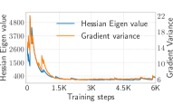
(a) ResNet101

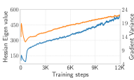
(b) VGG11

Figure 4: We compute the largest eigenvalue of second-order Hessian on every iteration along with first-order gradient variance. Changes in eigenvalue of the Hessian help detect critical periods, and it can be approximated with the variance of first-order gradients. The latter has a significantly lower computational overhead.

Summary: Gradients get smaller and eventually saturate, but the exact magnitude and trajectory of gradient progression varies for a DNN, dataset and DNN-specific hyperparameters.

III Design and Implementation

In this work, we leverage both the parallel and statistical aspect of DDP training by developing a flexible communication strategy to perform either synchronous or local-SGD updates based on their significance. Parallel efficiency is improved via local-SGD where workers apply their respective updates locally and avoid communication which reduces iteration time and speeds up training. When gradients change significantly, statistical efficiency is prioritized by synchronizing updates among all workers. Although this increases the iteration time due to communication, the aggregated gradients are less noisy than the locally computed gradients. These averaged updates are then applied globally to produce a model state consistent across all workers.

III-A Detecting crucial updates in DNN training

Distributed training extends metrics like throughput and scale-out factor from fields like HPC and parallel computing to measure the parallel efficiency of collaboratively training a model across various workers. However, DNN training has a statistical aspect as well that is non-linear; some updates are more critical than others towards overall model learning and generalization. As seen previously in §II-E, gradients change considerably in the early phase and at certain critical regions.

Recent works have demonstrated that gradient variance, or signal-to-noise ratio between the local and aggregated updates can serve as a useful indicator of the statistical efficiency of DDP training [22, 23, 24]. In fact, there is a strong correlation between the changes in the eigen values of the second-order Hessian [25] and the norm of first-order gradients [27]. Computing gradient norm is computationally feasible as it can easily be incorporated in backpropagation, while computing the Hessian is very expensive from a computational standpoint. We measure the significance of each update by tracking changes in gradient norm on every iteration. Relative gradient change between consecutive steps can be estimated from the $\mathbb{L}{2}$-norm of gradient $\nabla\mathcal{F}$ at steps $(\mathit{i}-1)$ and $\mathit{i}$, as shown in Eqn. (2):

$$\triangle(g_{i})=\bigg{|}\dfrac{\mathbb{E}[||\nabla\mathcal{F}_{(i)}||^{2}]-\mathbb{E}[||\nabla\mathcal{F}_{(i-1)}||^{2}]}{\mathbb{E}[||\nabla\mathcal{F}_{(i-1)}||^{2}]}\bigg{|}$$ (2)

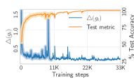
(a) ResNet101

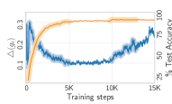
(b) VGG11

(c) AlexNet

(d) Transformer

Figure 5: Correlation between relative gradient change and model convergence in BSP. A rise or decline in test accuracy or perplexity is accompanied by changes in the gradients as well. As convergence plateaus, so does $\triangle(g_{i})$.

Gradients computed on a single iteration are noisy, so we use exponentially weighted moving average (EWMA) [43] for smoothing. We plot $\triangle(g_{i})$ at every iteration $i$ alongside the convergence curves in Fig. (5). The curves correspond to test accuracy for ResNet101, VGG11 and AlexNet (the higher, the better), and test perplexity for Transformer (the lower, the better). We apply EWMA with a window-size of 25 iterations and a smoothing factor of $N$/100, or 0.16 for a 16-node cluster. The plots highlight the correlation between critical updates (measured by $\triangle(g_{i})$) and model progression during training. The particularly volatile phases are shown as shaded in Fig. (5). For Transformer, we omit perplexity for first 8K iterations as it was very high initially and fell sharply in that phase.

Fig. (5a) and Fig. (5d) shows how gradients change in ResNet101 and Transformer as the accuracy/perplexity changes sharply. The sudden peak in ResNet101 after 10K steps corresponds to learning rate decay. The first 10K steps in Transformer where the perplexity fell aggressively, the associated gradients fall and rise sharply as well. The perplexity falls gradually after 13K iterations, as does the corresponding gradient change. As for AlexNet, Fig. (5c) shows how $\triangle(g_{i})$ varies gradually such that accuracy gains over the same set of iterations are gradual as well. The gradients for VGG11 in Fig. (5b) change rapidly in the first 5K steps as accuracy improves steeply in that phase. As accuracy saturates between iterations 5K and 10K, gradients stop changing as well and $\triangle(g_{i})$ flattens out in that phase. The accuracy then jumps up after 10Kth step due to learning rate decay alongside $\triangle(g_{i})$.

III-B $\delta$-based selective synchronization

Gradient changes tend to be more prominent with aggressive updates, and stabilize over the course of training. As a model converges, gradients stop changing as abruptly, as does $\triangle(g_{i})$. The maximum degree by which gradients vary depends on DNN size and complexity, weight initialization, among other hyperparameters. Denoting this extremum as $\mathcal{M}$=$max([\triangle(g_{i})]_{i=1}^{i=I})$ after running for $I$ iterations, gradient change then lies in the range $[0,\mathcal{M}]$.

With this intuition, it is thus logical to synchronize worker updates only when $\triangle(g_{i})$ changes considerably, and perform local updates to avoid communication otherwise. By choosing perceptively between synchronous and local updates, we try to balance the parallel and statistical efficiency of DDP training. Additionally, incorporating local-SGD updates in otherwise synchronous training allows for more exploration of the local minima by every worker which in turn can improve model generalization [37, 44]. By allowing workers to train locally, SelSync thus allows model replicas to explore their local latent space, while still bounding the divergence between local and global model states. The latter is located on the central PS node. SelSync proposes an effective and practical method to measure the significance of inter-iteration updates by imposing a threshold, denoted by $\delta$, on relative gradient change described as follows: use local-SGD updates if gradient change is below $\delta$ and synchronize updates if any of the workers’ $\triangle(g_{i})\geq\delta$. Threshold ‘$\delta$’ is set prior training launch such that $\delta$=0 implies fully synchronous training while setting a sufficiently large threshold ($\delta\geq\mathcal{M}$) trains with local-SGD only. In case of fully local-SGD training, workers never communicate with each other and explore only their respective local minimas. Fig. 6 illustrates how one can slide around $\delta$ between 0 and $\mathcal{M}$ to adjust the degree of training between synchronous and local updates with SelSync.

Figure 6: Adjusting threshold $\delta$ on relative gradient change. Choose BSP if $\triangle(g_{i})\geq\delta$ and local SGD if $<\delta$. Setting $\delta$=0 implies BSP training, while a very high $\delta$ trains only with local updates.

III-C Gradient vs. Parameter aggregation for SelSync

In BSP, synchronization can either be performed on the gradients or model parameters. They are equivalent in BSP assuming all workers initially started with the same model parameters. On PS, this is done by workers pulling initial model state from the central server prior training, while decentralized topologies can broadcast model parameters from one of the workers to all others in the cluster. Local models are thus consistent with the global state on every step in BSP as the same, aggregated set of updates are applied to each worker. In spite of their equivalence, gradient aggregation is more popular as gradients can be compressed [28, 29] via sparsification [30, 31, 32], quantization [33, 34] or low-rank updates [35]. Model parameters can be compressed via pruning [36] as well, although model generalization and compression factor achieved is comparatively subpar.

However, gradient aggregation (GA) and parameter aggregation (PA) are not equivalent in the context of semi-synchronous training; reducing model parameters instead of gradients tends to produce DNNs with better generalization performance. Since SelSync collects updates infrequently (depending on $\triangle(g_{i})$ and chosen $\delta$), GA can cause local models to diverge from the global state on the PS and thus, lead to model inconsistency across workers. The more the iterations are performed locally, the more local replicas can diverge as a result. This is because even though the same set of averaged gradients are applied to each worker in GA, the resultant parameters post-SGD update will be different across workers and may eventually become inconsistent, especially after workers have been training locally for many subsequent iterations. This increased divergence can thus deteriorate the test performance in semi-synchronous methods.

However, local training is not always bad; lettings workers train with local-SGD permits ample exploration of the local minima [37]. Adding PA on top of that ensures local weights are bounded to the global weights and do not fall into a local minima that is too far from the global state. Further, aggregating parameters during synchronization phase ensures model consistency across all workers. We empirically validate that PA achieves same or better convergence than GA across a variety of DNNs when training with SelSync.

III-D IID data partitioning for semi-synchronous training

BSP maximizes per-iteration work by processing a unique mini-batch on every worker and combining updates from those partitions. For example, training dataset $\mathcal{D}$ can be partitioned among 4 workers as $\mathcal{D}\supseteq\{$DP0, DP1, DP2, DP3$\}$, such that each partition resides on a single worker. We refer to this as Default data-partitioning or DefDP, depicted in Fig. (7a) where worker0 samples from partition DP0, worker1 from DP1, worker2 from DP2 and worker3 from DP3. This approach works well in BSP as every training sample is used at least once in each epoch to update model parameters.

(a) Default data-partitioning (DefDP) in a 4 worker cluster.

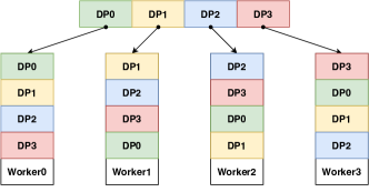
(b) SelSync data-partitioning (SelDP) in a 4 worker cluster.

Figure 7: Data-partitioning (DP) in distributed training. DefDP splits training data into as many partitions as the number of workers. SelDP partitions data as a circular queue whose head is rotated to a unique chunk on each worker.

However, such a partitioning scheme does not work well for semi-synchronous methods. Consider a DNN training with SelSync where most of the iterations favor local-SGD over synchronous updates. Every worker then optimizes the model for its local training subset only and fails to aggregate updates from other workers computed on different data partitions. Thus, local replicas are deprived of learning features from data partitions situated on other workers due to low or negligible communication. Even if aggregation is triggered occasionally, averaging diverge model can produce a resultant model of low quality [8]. Training DNNs with DefDP in semi-synchronous methods is somewhat analogous to training with unbalanced data in federated learning, which is detrimental to model convergence as well.

As part of SelSync, we propose a custom partitioning scheme tailored for techniques using a hybrid of local and synchronous updates. Instead of splitting data into unique and separate chunks, we shuffle dataset $\mathcal{D}$ on every worker based on its ID in the cluster (in case of decentralized training using allreduce collectives, this corresponds to a worker’s rank). So, worker0 computes on partitions ordered as $\{$DP0, DP1, DP2, DP3$\}$, worker1 processes in the order $\{$DP1, DP2, DP3, DP0$\}$, worker2 as $\{$DP2, DP3, DP0, DP1$\}$, while worker3 samples batches ordered as $\{$DP3, DP0, DP1, DP2$\}$. The shuffling operation is a one-time overhead that is executed prior training. Thus, SelSync data-partitioning, or SelDP ensures all training samples are available to every worker to train on. This partitioning scheme is illustrated in Fig. (7b). In this way, local model replicas will not be skewed from training with local-SGD for most iterations (say for SelSync with a high $\delta$-setting). On the other hand, when worker updates do synchronize, SelDP ensures each workers’ updates comes from a unique chunk and none of the workers redundantly process the same set of training samples for a given iteration. For e.g., if the very first iteration qualifies for synchronization, then worker0 processes a mini-batch from chunk DP0, worker1 processes from DP1, worker2 processes from DP2 and worker3 processes from DP3.

III-E Training on unbalanced and non-IID data

As seen in §II-B, distributed training suffers from model deterioration due to unbalanced and skewed data on account of its non-IIDness. To mitigate this issue, we extend randomized data-injection [39] and apply it in the context of semi-synchronous training when dealing with non-IID data. In data-injection, a random subset of workers communicate amongst themselves and share partial training data. Privacy risk is minimized by sharing data with only a fraction of workers randomly and on a per-iteration basis. Data-injection is configured as a tuple of ($\alpha,\beta$), where $\alpha$ is the fraction of workers chosen while $\beta$ is the proportion of worker batch-size to be shared. For e.g., an ($\alpha,\beta$) of (0.5, 0.5) implies half of the total workers are selected randomly to share half of their training samples, thus improving the overall data distribution in DDP training.

The mini-batch size is an important hyperparameter in DNN training. Naively applying data-injection can be harmful if the cluster-size is large. This is because the per-worker batch-size would then become undesirably large as well and degrade model generalization as commonly seen in large-batch training [26], [40]. To avoid this, we enforce the following constraint in SelSync: when dealing with on non-IID data, adjust worker batch-size to $b^{{}^{\prime}}$ such that cumulative batch-size after data-injection is same as the originally set batch-size $b$, shown in Eqn. (3) for a cluster of $N$ workers:

$$b^{{}^{\prime}}=\frac{b}{(1+\alpha\beta N)}$$ (3)

The communication overhead of data-injection is low; each iteration additionally communicates only ($\alpha\beta Nb^{\prime}$) times the size of an individual sample. For CIFAR10/100, each image is about 3Kb (kilobytes), and 10-150Kb in ImageNet-1K. Thus, data-injection with 16 workers and $b$ = 32 in a (0.5, 0.5) configuration incurs a transfer of 132Kb on CIFAR10/100 and 440-6600Kb with ImageNet-1K. This cost is negligible compared to the cost of exchanging model updates that span hundreds of megabytes or even gigabytes in modern DNNs. To apply data-injection in SelSync, we additionally append the $\delta$-threshold and denote a configuration as ($\alpha,\beta,\delta$). Privacy risk with data-injection is reduced due to $K$-anonymity [49] (for a cluster-size of ‘$K$’ workers). Since workers are chosen randomly at each iteration, privacy is preserved by not knowing from which of the $\left\lceil\alpha\cdot K\right\rceil$ from the total $K$ workers did the training samples came from for the current iteration.

Training with SelSync: With the target to achieve same or better convergence as BSP while avoiding expensive communication and thus accelerate training, we develop SelSync for DNN training over both IID and non-IID data distributions, described in detail under Alg. (1). We fashion SelSync over parameter server (PS) architecture where worker updates are coordinated through a central server. But SelSync will also work in a decentralized topology where workers communicate amongst each other using MPI-based collectives. Training begins at line 3 of Alg. (1) with the workers pulling initial model state from the PS using pullFromPS function.

1 Input: learning rate $\eta$, gradient change threshold $\delta$, cluster-size $N$, training data $\mathcal{D}_{n}$ on worker with id $n$

2 procedure train():

3       $w_{(n,0)}$ = pullFromPS() $\triangleright$ initialize parameters

4       for $i$=0,1,…$I$ on worker id $n$ $\triangleright$ training iterations 

5             bit [$N$] flags = 0 $\triangleright$ synchronization status

6             $d_{(i,n)}\in\mathcal{D}_{n}$ $\triangleright$ sample mini-batch from data

7             $g_{i}=\nabla\mathcal{F}(x_{(i,k)},w_{(n,i)})$ $\triangleright$ compute gradient at $i$

8             $\triangle(g_{i})$ = RelativeGradChange ($||g_{i}||^{2}$)

9             $w_{(n,i+1)}=w_{(n,i)}-\eta\cdot g_{i}$ $\triangleright$ apply local updates

10            

11            if $\triangle(g_{i})\geq\delta:$ 

12                   flags [$n$] = 1 $\triangleright$ synchronize called by worker $n$ as its gradient change exceeds $\delta$

13                  

14            flags = allgather_status(flags) $\triangleright$ call all-gather on flags such that index $n$ holds worker $n$’s synchronization status bit

15             if $1\in\textnormal{{flags}}:$ 

16                   pushToPS($w_{(n,i+1)}$) $\triangleright$ push local updates

17                   $w_{(n,i+1)}$ = pullFromPS() $\triangleright$ pull global

Algorithm 1 {Sel}ective {Sync}hronization

Given a mini-batch sampled from dataset $\mathcal{D}_{n}$ on worker $n$, we compute the local gradients and its variance, as shown in line 7 and 8. The relative gradient change is measured by keeping track of gradient variance via RelativeGradChange in the algorithm. This function calculates and stores gradient variance at every iteration, applies EWMA smoothing, and computes the relative gradient change as shown in Eqn. (2). The local gradients are then used to update model parameters locally (line 9). To keep track of $\triangle(g_{i})$ across all workers, we initialize a flags array of length $N$ (for the total workers in the cluster). All elements of the array are reset to 0 at the beginning of each iteration (line 5); a bit value of 0 at index $n$ in flags implies $\triangle(g_{i})$ of worker with id $n$ is below threshold $\delta$ and thus, wants to perform SGD update only locally. Similarly, a bit value of 1 at index $n$ in flags means worker $n$’s relative gradient change exceeds the threshold and wants to communicate its update with other workers. We refer to this as the synchronization status of a worker. Lines 10-11 show that if $\triangle(g_{i})$ on worker $n$ is greater than $\delta$, we flip the corresponding bit at index $n$ to 1. We then call all-gather to communicate each worker’s synchronization bit to every other worker in the cluster (line 12). If any synchronization bit in the flags array is 1 post all-gather, we communicate gradients among the workers. Since we only exchange a single bit corresponding to each worker, the total communication volume of this step is just $(N-1)$ bits on every worker (in a cluster of size $N$). This op had a negligible overhead in our evaluation ($\approx$ 2-4 ms). If any of the bits in flags is 1, we synchronize by pushing local parameters of every worker to the PS via pushToPS function, and pulling updated model parameters: $w_{(n,i+1)}=\sum_{n=1}^{N}w_{(n,i)}/N$, i.e., perform parameter aggregation. Thus, local replicas remain consistent with the global model state as they all synchronize if even a single worker chooses synchronization over local-SGD. On the other hand, we train with local-SGD if all the bits of flags array are zero for a given iteration.

The dataset $\mathcal{D}_{n}$ at line 6 in Alg. (1) is treated differently based on its IID or non-IID properties. When training on IID data, we implement SelDP partitioning for SelSync by reordering and partitioning data on worker $n$ by first splitting training data $\mathcal{D}$ into $N$ equal-sized chunks. SelDP uses these partitions and works as a circular queue where the queue head on each worker is rotated to a position corresponding to its id $n$. When dealing with non-IID data, we apply data-injection on worker $n$ by randomly pinging a subset of workers and pulling data, as determined by ($\alpha,\beta,\delta$) parameters. To keep the batch-size from blowing up when $N$ is large, we reduce local mini-batch size to $b^{\prime}$ of Eqn. (3). We implement data-injection via point-to-point (P2P) communication, i.e., send/push and recv/pull calls.

It is also worth pointing out that the synchronization steps currently implemented as PS strategy can be switched with an alternative communication operation. For e.g., pullFromPS and pushToPS function calls in Alg. (1) can be easily swapped for an AllReduce collective. The bandwidth cost of PS strategy increases with the number of workers, while allreduce collectives based on decentralized topology like ring or tree are bandwidth-optimal and logarithmic bandwidth-optimal respectively [50]. By trading for more optimal communication strategies, training speedup can be further improved. The main appeal with SelSync’s approach is its effectiveness in deeming which updates are important to communicate and which to use locally, thus switching between local and synchronous updates.

IV Experimental Evaluation

IV-A Cluster setup and workload specifications

We test SelSync on a system of 4 servers, each equipped with 48-core Intel Xeon E5-2560 CPU, 128GB system memory and 4 NVIDIA V100 GPUs. To ensure resource isolation and minimum interference, we deploy a cluster of 16 CUDA-compatible nvidia-docker containers such that each container is allocated 8vCPUs, 24GB system memory and 1 NVIDIA V100 GPU. The worker containers push/pull their updates to/from a PS container with 12vCPUs and 32GB system memory. Communication between PS and worker containers is enabled via docker swarm configured over a 5Gbps NIC.

Data for IID training: CIFAR10/100 contains 50K train and 10K test images with 10 and 100 labels respectively. ImageNet-1K has 1.28 million training and 50K test images spanning across 1K class labels. WikiText-103 has 100 million tokens of verified and featured articles from Wikipedia [38].

Data for non-IID training: To evaluate performance in non-IID settings, we split CIFAR10/100 across 10 workers with 1 and 10 labels per-worker for CIFAR10 and CIFAR100.

DNNs and hyperparameters: We train ResNet101 on CIFAR10 and report top-1 test accuracy from training with per-worker batch-size 32 and SGD optimizer with initial lr 0.1, weight decay 0.0004 and momentum 0.9. We progressively decay the lr by 10$\times$ after 110 and 150 epochs. VGG11 measures top-1 test accuracy on CIFAR100 with batch-size 32 and SGD optimizer with momentum 0.9, weight decay 0.0005 and initial lr 0.01 that decays by 10$\times$ after epoch 50 and 75. AlexNet trains on ImageNet-1K to report top-5 test accuracy with batch-size 128, Adam optimizer [3] and fixed lr of 0.0001. Lastly, we train Transformer on WikiText-103 where the encoder has 2 hidden layers of dimension 200, 2 heads, an embedding dimension of 200, dropout 0.2 and 35 bptt (backpropagation through time) steps. We set per-worker batch-size to 20 and use SGD optimizer with initial lr 2.0 that decays by a factor of 0.8 every 2000 iterations and report the test perplexity, i.e., exponential of the loss function.

Comparing SelSync with SOTA learning algorithms: The same cluster of 16 workers and 1 PS is also used to evaluate BSP, FedAvg and SSP. We train with BSP across all 16 workers using the default partitioning scheme (DefDP) and updates are aggregated on the PS at every iteration. SelSync is deployed with different thresholds; a $\delta$ of 0.25, 0.3 or 0.5. We launch FedAvg with four different configurations by varying the fraction of participating workers (C) and the synchronization factor (E): ($C$, $E$) $\rightarrow$ (1, 0.25), (1, 0.125), (0.5, 0.25) and (0.5, 0.125). This means we either use all or just half of the participating workers during communication phase in FedAvg, while aggregation is done either 4 or 8 times in every epoch at uniform intervals. We deploy SSP with two staleness thresholds: 100 and 200 steps. The chosen $s$ values are large enough to not be a frequent synchronization barrier, while still small enough to not let worker models diverge too far from the global model.

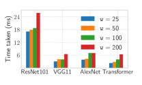
(a) $\triangle(g_{i})$ computation overhead

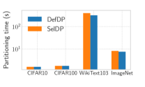
(b) Data-partitioning overhead

Figure 8: (a) Overhead of computing gradient variance and applying EWMA smoothing for different window-sizes. (b) Average time taken across workers to shuffle and create SelDP. This is a one-time overhead incurred as part of data-batching and loading in the preprocessing stage.

IV-B Computational overhead of SelSync

The RelativeGradChange function from Alg. (1) applies smoothing because gradients computed over a mini-batch between consecutive iterations can be noisy. This overhead is exclusive to SelSync as $\triangle(g_{i})$ is not computed in BSP, FedAvg or SSP. As the window-size used for smoothing becomes larger, this overhead rises as well (shown in Fig. (8a)). Time increases from 17 to 26ms in ResNet101 as the window-size increases from 25 to 200 steps; a jump of about 53%. A window of 25 iterations takes only about 3.1, 3.9 and 2.3ms on VGG11, AlexNet and Transformer respectively. On increasing their windows to 200, their respective latencies increase by 110%, 79% and 178%. Although this cost increases with larger windows, this latency is considerably lower than the typical computation and communication cost of distributed training. Besides, we observed in our evaluation that a $w$ = 25 sufficed for detecting inter-iteration gradient changes. We use this window-size in our experiments, unless specified otherwise.

We evaluate the overhead of Selsync-data partitioner (SelDP) in this section as well. We compare the overhead of the two partitioning schemes for SelSync in Fig. (8b). Instead of splitting the data into unique, equal-sized chunks, SelDP rearranges the partitions based on worker id in the cluster. For CIFAR10/100 datasets, this additional operation does not incur considerable overhead as loading time of SelDP and DefDP are nearly identical. This is because size of these datasets is not that big to pose a considerable overhead to reorder and shuffle. For bigger datasets like ImageNet-1K and WikiText-103, SelDP had a higher processing time over the default partitioning scheme. However, the margin is only of a few seconds and the partitioning operation is a one-time overhead incurred before the actual training begins.

IV-C Training SelSync with SelDP vs. DefDP

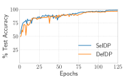
(a) ResNet101

(b) VGG11

(c) AlexNet

(d) Transformer

Figure 9: Test accuracy/perplexity curves of SelSync for $\delta$ = 0.25 with SelDP and DefDP. We perform gradient aggregation during synchronization phase. For the same epochs, SelDP achieves better generalization/test performance.

In this section, we deploy SelSync with $\delta$ = 0.25 and see how different models converge with our custom partitioning vs. the default scheme typically used in DDP training. We plot the convergence curves in Fig. (9) (i.e., test accuracy or perplexity vs. epochs). During the synchronization phase, we perform gradient aggregation on the PS and return reduced gradients back to the workers to apply locally. By the end of epoch 125, ResNet101 converged to 97.6% test accuracy on SelDP and 96.8% on the default scheme. CIFAR100 partitioned with DefDP performed poorly on VGG11 with only 64.1% accuracy, while SelDP converged to 90.86% after 90 epochs. We see more performance degradation in VGG11 with DefDP compared to ResNet101 as the training data of the former has more labels to evaluate; CIFAR100 vs. CIFAR10. Although VGG11 is larger, ResNet101 is a skip-connection based architecture that generalizes better compared to the simpler convolution-based architecture [12]. With SelDP partitioning, AlexNet converged to 81.1% top-5 test accuracy while SelSync with DefDP did not improve beyond 61.2%. Training Transformer on SelSync with SelDP attained 92.6 while DefDP converged to 94.91 test perplexity near the end of half an epoch. The perplexity before epochs 0.3 and 0.38 for the two partitioning schemes is omitted in Transformer as it was very high initially and fell rapidly in that phase.

Summary: SelDP outperforms DefDP in semi-synchronous training. This is because many updates are performed locally and not aggregated among workers. With DefDP, worker replicas only train on data local to them and fail to learn from partitions located on other workers. As a result, local models tend to diverge away from the global model. With SelDP, each worker has access to the entire training data, albeit in a different order. This ensures the local model weights do not significantly diverge in their local minima.

(a) ResNet101

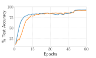
(b) VGG11

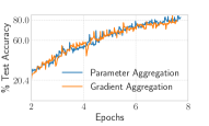
(c) AlexNet

(d) Transformer

Figure 10: Convergence curves comparing gradients (GA) vs. parameter aggregation (PA) in SelSync with $\delta$ = 0.25. For the same epochs, PA achieved better accuracy in settings with a learning rate decay schedule. Interestingly, both performed similarly in AlexNet where the learning rate was fixed.

IV-D SelSync with Gradient vs. Parameter Aggregation

We fix every other setting and deploy SelSync where we only change the aggregation mechanism: gradient aggregation (GA) vs. parameter aggregation (PA). We set $\delta$ = 0.25, partition training data with SelDP and compare their accuracy/perplexity over a fixed set of epochs. The convergence plots are shown in Fig. (10). By the end of 100 epochs, ResNet101 converges to 96.8% test accuracy with GA and 98.52% with PA, an improvement of 1.72% with parameter averaging. VGG11 with GA attained 90.86% accuracy and 91.42% with PA at epoch 60, about 0.56% more than GA for the same amount of training. We see in Fig. (10d) that both GA and PA converge to a perplexity of 90.0 for Transformer; however, SelSync with PA reached there in 0.3 epochs while GA took 130% more iterations to converge. AlexNet, the only model trained with a fixed learning rate, had similar convergence trajectory on both GA and PA.

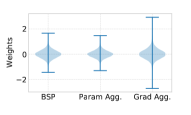
(a) Epoch 25

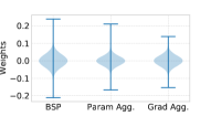
(b) Epoch 50

Figure 11: Comparing distribution density of model weights while training independently via BSP, SelSync with Param Agg. (PA) and Grad Agg. (GA). Distribution between model weights is compared over epochs 25 and 50 for layer layer1_1_conv1_weight of ResNet101. BSP and SelSync with PA have similar distributions compared to SelSync with GA.

The better generalization of SelSync with PA over GA can be seen from the distribution of model parameters of the two approaches and how well they align with the parameter distributions had we trained with BSP. For three independent runs of ResNet101 with BSP, SelSync with GA and PA, Fig. (11) shows the parameter density estimates plotted at epochs 25 and 50. On 25th epoch, BSP and PA have similar distributions, whereas parameters of GA were comparatively spread apart. As training continues (around epoch 50), parameter distribution of GA is much smaller and narrower than both BSP and SelSync with PA. Thus, we see that from the distributions that weights diverge more with gradient aggregation. Comparatively, parameter aggregation was much more aligned with BSP training. This is because by aggregating parameters during synchronization phase, we bound the divergence between local models on the workers and the global model on the PS.

IV-E Training with IID and non-IID data

Model	Method	Iterations	LSSR	Acc./PPL	Conv. Diff.	Outperform BSP ?	Overall speedup
ResNet101	BSP	22.8K	0.0	98.5%	0.0%	N/A	1$\times$
	FedAvg (1, 0.25)	63.4K	0.979	98.55%	+0.05%	True	2.59$\times$
	FedAvg (1, 0.125)	57.1K	0.959	98.6%	+0.1%	True	2.55$\times$
	FedAvg (0.5, 0.25)	66.8K	0.979	94.4%	-4.1%	False	-
	FedAvg (0.5, 0.125)	62.8.1K	0.959	95.5%	-3.0%	False	-
	SSP $s$ = 100	54.8K	-	93.8%	-4.7%	False	-
	SSP $s$ = 200	59.4K	-	93.33%	-5.17%	False	-
	SelSync $\delta$ = 0.3	42.2K	0.829	98.62%	+0.12%	True	2.03$\times$
	SelSync $\delta$ = 0.5	53.2K	0.846	98.56%	+0.06%	True	1.67$\times$
VGG11	BSP	10.8K	0.0	90.9%	0.0%	N/A	1$\times$
	FedAvg (1, 0.25)	17.4K	0.979	87.56%	-3.34%	False	-
	FedAvg (1, 0.125)	20.2K	0.959	88.2%	-2.7%	False	-
	FedAvg (0.5, 0.25)	19.6K	0.979	84.6%	-6.3%	False	-
	FedAvg (0.5, 0.125)	21.1K	0.959	85.16%	-5.74%	False	-
	SSP $s$ = 100	11.8K	-	68.72%	-22.18%	False	-
	SSP $s$ = 200	12.2K	-	68.78%	-22.12%	False	-
	SelSync $\delta$ = 0.3	72.4K	0.912	91.33%	+0.43%	True	6.16$\times$
	SelSync $\delta$ = 0.5	81.2K	0.937	91.32%	+0.42%	True	13.75$\times$
AlexNet	BSP	106.5K	0.0	85.15%	0.0%	N/A	1$\times$
	FedAvg (1, 0.25)	118K	0.997	77.15%	-8.0%	False	-
	FedAvg (1, 0.125)	124K	0.993	78.2%	-6.95%	False	-
	FedAvg (0.5, 0.25)	115.6K	0.997	75.6%	-9.55%	False	-
	FedAvg (0.5, 0.125)	121.4K	0.993	76.67%	-8.48%	False	-
	SSP $s$ = 100	111.5K	-	86.52%	+1.37%	True	4.53$\times$
	SSP $s$ = 200	113.2K	-	85.8%	+0.65%	True	4.47$\times$
	SelSync $\delta$ = 0.3	95.8K	0.954	86.72%	+1.57%	True	4.62$\times$
	SelSync $\delta$ = 0.5	106.8K	0.966	85.93%	+0.78%	True	4.63$\times$
Transformer	BSP	28K	0.0	90.02	0.0%	N/A	1$\times$
	FedAvg (1, 0.25)	112.1K	0.998	89.96	+0.06	True	1.99$\times$
	FedAvg (1, 0.125)	104.2K	0.999	90.01	+0.01	True	2.14$\times$
	FedAvg (0.5, 0.25)	118K	0.999	91.67	-1.65	False	-
	FedAvg (0.5, 0.125)	111.6K	0.998	91.2	-1.18	False	-
	SSP $s$ = 100	110K	-	89.98	+0.04	True	2.02$\times$
	SSP $s$ = 200	116.2K	-	90.0	+0.0	True	1.92$\times$
	SelSync $\delta$ = 0.3	38.6K	0.725	89.91	+0.11	True	2.42$\times$
	SelSync $\delta$ = 0.5	46.1K	0.733	89.97	+0.05	True	2.06$\times$

TABLE I: DNN Performance Across SelSync, BSP, FedAvg and SSP. Convergence Difference (Conv. Diff.) and Speedup w.r.t. BSP.

IID training: To measure the fraction of training using local updates versus steps that are synchronized among workers, we define a metric called local-to-synchronous step ratio, or LSSR measured as:

$$\text{LSSR}=\frac{\texttt{steps}_{local}}{\texttt{steps}_{local}+\texttt{steps}_{bsp}}$$ (4)

If all updates are local, then $\mathtt{steps}_{bsp}$=0 and LSSR=1. For BSP training, LSSR = 0 as all the updates are synchronous and there are no local updates. LSSR essentially measures communication reduction w.r.t. BSP as $1/(1-\text{LSSR})$ for the same number of iterations/epochs. For e.g., LSSR of 0.9 implies a communication reduction of 10$\times$ over BSP. LSSR scores do not apply to SSP as workers push updates to the PS asynchronously and do not synchronize them. When staleness threshold is crossed, faster workers wait for slower workers to catch-up. There is no explicit gradient summation/averaging in SSP, thus a metric like LSSR doesn’t apply. Table (I) compares SelSync with BSP, FedAvg and SSP. We run each model until the accuracy/perplexity does not improve any further and note the corresponding iterations taken and the LSSR scores (if applicable). We measure convergence and speedup w.r.t. BSP as many semi-synchronous methods do provide training speedups, but not necessarily meet the same convergence targets as BSP. Results from the ‘Overall speedup’ column of Table (I) are omitted for settings that failed to converge to the same accuracy as BSP.

For ResNet101, we see that SelSync and few configurations of FedAvg achieve higher accuracy than BSP. The improvement over BSP comes from abundant exploration of the local minima on individual workers which results in better generalization performance [37]. However, too much local exploration as well as infrequent (from $E$) and partial (from $C$) aggregation can increase the divergence between the local and global model state, as seen in FedAvg for ($C,E$) values (0.5,0.25) and (0.5,0.125). Here, local updates were collected from only half the workers during synchronization. FedAvg with $C$=1 performed well even with high LSSR scores ($\approx$ 0.95-0.97) as ResNet101 is an over-parameterized network for a dataset like CIFAR10, and was thus more robust to local training with FedAvg. SelSync with $\delta$ = 0.3 and 0.5 had LSSR scores 0.83-0.84. Thus, overall speedup over BSP was slightly higher for FedAvg on account of its higher LSSR scores; around 2.59$\times$ while SelSync was up to 2$\times$. SSP failed to beat BSP because asynchronously pulling/pushing updates from/to the PS on a layer-by-layer basis introduced considerable staleness while training ResNet101.

A simpler convolutional network like VGG11 failed to achieve BSP-level accuracy with both FedAvg and SSP. SelSync attained 0.43% more accuracy over BSP and reduced training time by up to 13.75$\times$ due to high LSSR scores ($\approx$ 0.91-0.93). They are however lower than the LSSR scores of FedAvg because SelSync intelligently switches between synchronous and local updates based on their significance. This is also why SelSync gets better test accuracy than BSP while FedAvg and SSP failed to do so.

AlexNet on ImageNet-1K failed to converge across all FedAvg configurations. Since we set $E$ as the aggregation frequency in an epoch, the number of synchronization calls made with FedAvg were too low on account of large dataset size of 1.28 million samples. This can also be seen from the extremely high LSSR scores ($\approx$ 0.99) and thus, model trained locally for almost all iterations and learned features only from its local data. Due to smaller size and fewer layers of AlexNet, staleness was not an issue with SSP-based training with either of the $s$-thresholds. By asynchronously pushing and pulling updates to/from the PS, workers were also able to learn features from partitions on other workers, thus further improving the test accuracy. SSP attained up to 1.37% better accuracy than BSP while speeding up training by 4.53$\times$. SelSync was 4.63$\times$ faster and had 1.57% better accuracy than BSP. The speedup came from synchronizing only the crucial updates and performing 95-96% updates locally (as can be seen from the LSSR scores).

Last, Transformer with $C$ = 1 in FedAvg converged to a better perplexity than BSP while being 2.14$\times$ faster, courtesy of its high LSSR scores. SSP also successfully beat BSP, and converged 2$\times$ faster due to its asynchronous execution. SelSync trained for roughly 39-46K steps and synchronized about 26% of those iterations. By doing so, it converged to even lower perplexity than BSP while accelerating training by up to 2.42$\times$.

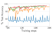
(a) ResNet101 on CIFAR10

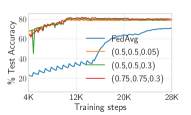
(b) VGG11 on CIFAR100

Figure 12: Data-injection in SelSync for different ($\alpha,\beta,\delta$) configurations vs. FedAvg on non-IID data.

Non-IID training: We now compare convergence between FedAvg and SelSync in non-IID settings. We choose three data-injection configurations ($\alpha,\beta,\delta$) to execute SelSync: (0.5, 0.5, 0.05), (0.5, 0.5, 0.3) and (0.75, 0.75, 0.3). As per Eqn. (3), we set $b^{\prime}$ = 11 to keep $b$ = 32 for the first two configurations and $b^{\prime}$ = 6 for the last. With non-IID data, FedAvg oscillated between 60-70% test accuracy for ResNet101, and saturated to 70% accuracy on VGG11. As ($\alpha,\beta,\delta$) increases, the corresponding data distribution improves and thus, so does the accuracy. SelSync configuration (0.75, 0.75, 0.3) thus achieved the maximum accuracy, followed by (0.5, 0.5, 0.3) and (0.5, 0.5, 0.05) in respective order. We thu see that Data-injection works well specifically for SelSync and generally in the context of semi-synchronous training.

V Conclusion

From Table (I), we see that BSP takes least number of steps to converge since it performs maximum work per-step by combining updates from all workers. However, it also suffers from high communication overheads to collect and distribute back updates. On the other hand, FedAvg provides decent speedups due to its high LSSR scores, however, the ($C,E$) configuration that provides maximum speedup or even convergence guarantees varies for each DNN and dataset. We saw in our evaluation that naively aggregating updates after fixed steps/epochs does not always yield the same convergence as BSP. Although workers communicate with the PS asynchronously in SSP, pushing/pulling updates for large and deeper models to/from the PS introduces staleness issues that either slows-down or even saturates convergence. Both FedAvg and SSP take more steps than BSP as they perform lesser work per-training step (i.e., $b$ vs. $Nb$ samples processed on each step). Across all models, SelSync achieved better accuracy/perplexity than BSP by selectively synchronizing updates that were deemed critical, applied updates locally otherwise. The relative gradient change metric $\triangle(g_{i})$ thus serves as an effective indicator of measuring the significance of each update in DNN training. With its high LSSR scores, SelSync eliminates considerable communication cost in the training phase and allows workers to explore local minima more than BSP, while still bounding the divergence between local and global model through frequent synchronization.

References

- [1] Ruder, S. (2016). An overview of gradient descent optimization algorithms. ArXiv, abs/1609.04747.
- [2] Nesterov, Y. (1983). A method for solving the convex programming problem with convergence rate . Proceedings of the USSR Academy of Sciences, 269, 543-547.
- [3] Kingma, D.P., and Ba, J. (2014). Adam: A Method for Stochastic Optimization. CoRR, abs/1412.6980.
- [4] Li, M., Andersen, D.G., Park, J.W., Smola, A., Ahmed, A., Josifovski, V., Long, J., Shekita, E.J., and Su, B. (2014). Scaling Distributed Machine Learning with the Parameter Server. BigDataScience ’14.
- [5] J. D. Owens, M. Houston, D. Luebke, S. Green, J. E. Stone and J. C. Phillips, ”GPU Computing,” in Proceedings of the IEEE, vol. 96, no. 5, pp. 879-899, May 2008, doi: 10.1109/JPROC.2008.917757.
- [6] Gustafson, J.L. (1988). Reevaluating Amdahl’s law. Commun. ACM, 31, 532-533.
- [7] Li, T., Sahu, A., Talwalkar, A., and Smith, V. (2019). Federated Learning: Challenges, Methods, and Future Directions. IEEE Signal Processing Magazine, 37, 50-60.
- [8] McMahan, H.B., Moore, E., Ramage, D., Hampson, S., and Arcas, B.A. (2016). Communication-Efficient Learning of Deep Networks from Decentralized Data. International Conference on Artificial Intelligence and Statistics.
- [9] Krizhevsky, A. (2009). Learning Multiple Layers of Features from Tiny Images.
- [10] pytorch.org/vision/0.12/generated/torchvision.datasets.ImageFolder.html
- [11] Vaswani, A., Shazeer, N.M., Parmar, N., Uszkoreit, J., Jones, L., Gomez, A.N., Kaiser, L., and Polosukhin, I. (2017). Attention is All you Need. ArXiv, abs/1706.03762.
- [12] He, K., Zhang, X., Ren, S., and Sun, J. (2015). Deep Residual Learning for Image Recognition. 2016 IEEE Conference on Computer Vision and Pattern Recognition (CVPR), 770-778.
- [13] Simonyan, K., and Zisserman, A. (2014). Very Deep Convolutional Networks for Large-Scale Image Recognition. CoRR, abs/1409.1556.
- [14] Krizhevsky, A., Sutskever, I., and Hinton, G.E. (2012). ImageNet classification with deep convolutional neural networks. Communications of the ACM, 60, 84 - 90.
- [15] Deng, J., Dong, W., Socher, R., Li, L., Li, K., and Fei-Fei, L. (2009). ImageNet: A large-scale hierarchical image database. 2009 IEEE Conference on Computer Vision and Pattern Recognition, 248-255.
- [16] Tyagi, S., and Sharma, P. (2020). Taming Resource Heterogeneity In Distributed ML Training With Dynamic Batching. 2020 IEEE International Conference on Autonomic Computing and Self-Organizing Systems (ACSOS), 188-194.
- [17] Merity, S., Xiong, C., Bradbury, J., and Socher, R. (2016). Pointer Sentinel Mixture Models. ArXiv, abs/1609.07843.
- [18] Frankle, J., Schwab, D.J., and Morcos, A.S. (2020). The Early Phase of Neural Network Training. ArXiv, abs/2002.10365.
- [19] Achille, A., Rovere, M., and Soatto, S. (2017). Critical Learning Periods in Deep Neural Networks. ArXiv, abs/1711.08856.
- [20] Jastrzebski, S., Kenton, Z., Ballas, N., Fischer, A., Bengio, Y., and Storkey, A.J. (2018). On the Relation Between the Sharpest Directions of DNN Loss and the SGD Step Length. arXiv: Machine Learning.
- [21] McCandlish, S., Kaplan, J., Amodei, D., and Team, O.D. (2018). An Empirical Model of Large-Batch Training. ArXiv, abs/1812.06162.
- [22] Mai, L., Li, G., Wagenländer, M., Fertakis, K., Brabete, A., and Pietzuch, P.R. (2020). KungFu: Making Training in Distributed Machine Learning Adaptive. USENIX Symposium on Operating Systems Design and Implementation.
- [23] Qiao, A., Neiswanger, W., Ho, Q., Zhang, H., Ganger, G.R., and Xing, E.P. (2020). Pollux: Co-adaptive Cluster Scheduling for Goodput-Optimized Deep Learning. ArXiv, abs/2008.12260.
- [24] Johnson, T.B., Agrawal, P., Gu, H., and Guestrin, C. (2020). AdaScale SGD: A User-Friendly Algorithm for Distributed Training. ArXiv, abs/2007.05105.
- [25] Sagun, L., Bottou, L., and LeCun, Y. (2016). Eigenvalues of the Hessian in Deep Learning: Singularity and Beyond. arXiv: Learning.
- [26] Hoffer, E., Hubara, I., and Soudry, D. (2017). Train longer, generalize better: closing the generalization gap in large batch training of neural networks. ArXiv, abs/1705.08741.
- [27] Agarwal, S., Wang, H., Lee, K., Venkataraman, S., and Papailiopoulos, D. (2020). Accordion: Adaptive Gradient Communication via Critical Learning Regime Identification. ArXiv, abs/2010.16248.
- [28] Cheng, Y., Wang, D., Zhou, P., and Tao, Z. (2017). A Survey of Model Compression and Acceleration for Deep Neural Networks. ArXiv, abs/1710.09282.
- [29] Tyagi, S., and Swany, D.M. GraVAC: Adaptive Compression for Communication-Efficient Distributed DL Training. IEEE CLOUD 2023.
- [30] Alistarh, D., Hoefler, T., Johansson, M., Khirirat, S., Konstantinov, N., and Renggli, C. (2018). The Convergence of Sparsified Gradient Methods. Neural Information Processing Systems.
- [31] Shi, S., Wang, Q., Zhao, K., Tang, Z., Wang, Y., Huang, X., and Chu, X. (2019). A Distributed Synchronous SGD Algorithm with Global Top-k Sparsification for Low Bandwidth Networks. 2019 IEEE 39th International Conference on Distributed Computing Systems (ICDCS), 2238-2247.
- [32] Lin, Y., Han, S., Mao, H., Wang, Y., and Dally, W.J. (2017). Deep Gradient Compression: Reducing the Communication Bandwidth for Distributed Training. ArXiv, abs/1712.01887.
- [33] Wen, W., Xu, C., Yan, F., Wu, C., Wang, Y., Chen, Y., and Li, H.H. (2017). TernGrad: Ternary Gradients to Reduce Communication in Distributed Deep Learning. NIPS.
- [34] Seide, F., Fu, H., Droppo, J., Li, G., and Yu, D. (2014). 1-bit stochastic gradient descent and its application to data-parallel distributed training of speech DNNs. Interspeech.
- [35] Vogels, T., Karimireddy, S.P., and Jaggi, M. (2019). PowerSGD: Practical Low-Rank Gradient Compression for Distributed Optimization. Neural Information Processing Systems.
- [36] Srinivas, S., and Babu, R.V. (2015). Data-free Parameter Pruning for Deep Neural Networks. British Machine Vision Conference.
- [37] Zhang, S., Choromańska, A., and LeCun, Y. (2014). Deep learning with Elastic Averaging SGD. NIPS.
- [38] Merity, S., Xiong, C., Bradbury, J., and Socher, R. (2016). Pointer Sentinel Mixture Models. ArXiv, abs/1609.07843.
- [39] Tyagi, S., and Swany, D.M. (2022). ScaDLES: Scalable Deep Learning over Streaming data at the Edge. 2022 IEEE International Conference on Big Data (Big Data), 2113-2122.
- [40] Keskar, N.S., Mudigere, D., Nocedal, J., Smelyanskiy, M., and Tang, P.T. (2016). On Large-Batch Training for Deep Learning: Generalization Gap and Sharp Minima. ArXiv, abs/1609.04836.
- [41] Paszke, A., Gross, S., Massa, F., Lerer, A., Bradbury, J., Chanan, G., Killeen, T., Lin, Z., Gimelshein, N., Antiga, L., Desmaison, A., Köpf, A., Yang, E., DeVito, Z., Raison, M., Tejani, A., Chilamkurthy, S., Steiner, B., Fang, L., Bai, J., and Chintala, S. (2019). PyTorch: An Imperative Style, High-Performance Deep Learning Library. ArXiv, abs/1912.01703.
- [42] Thakur, R., Rabenseifner, R., and Gropp, W. (2005). Optimization of Collective Communication Operations in MPICH. The International Journal of High Performance Computing Applications, 19, 49 - 66.
- [43] Hunter, J.S. (1986). The exponentially weighted moving average. Journal of Quality Technology, 18, 203-210.
- [44] Zhao, Y., Li, M., Lai, L., Suda, N., Civin, D., and Chandra, V. (2018). Federated Learning with Non-IID Data. ArXiv, abs/1806.00582.
- [45] Harlap, A., Narayanan, D., Phanishayee, A., Seshadri, V., Devanur, N.R., Ganger, G.R., and Gibbons, P.B. (2018). PipeDream: Fast and Efficient Pipeline Parallel DNN Training. ArXiv, abs/1806.03377.
- [46] Sun, P., Feng, W., Han, R., Yan, S., and Wen, Y. (2019). Optimizing Network Performance for Distributed DNN Training on GPU Clusters: ImageNet/AlexNet Training in 1.5 Minutes. ArXiv, abs/1902.06855.
- [47] Micikevicius, P., Narang, S., Alben, J., Diamos, G.F., Elsen, E., García, D., Ginsburg, B., Houston, M., Kuchaiev, O., Venkatesh, G., and Wu, H. (2017). Mixed Precision Training. ArXiv, abs/1710.03740.
- [48] Peng, Y., Zhu, Y., Chen, Y., Bao, Y., Yi, B., Lan, C., Wu, C., and Guo, C. (2019). A generic communication scheduler for distributed DNN training acceleration. Proceedings of the 27th ACM Symposium on Operating Systems Principles.
- [49] Sweeney, L. (2002). k-Anonymity: A Model for Protecting Privacy. Int. J. Uncertain. Fuzziness Knowl. Based Syst., 10, 557-570.
- [50] Agarwal, S., Wang, H., Venkataraman, S., and Papailiopoulos, D. (2021). On the Utility of Gradient Compression in Distributed Training Systems. ArXiv, abs/2103.00543.
- [51] Ho, Qirong, et al. “More Effective Distributed ML via a Stale Synchronous Parallel Parameter Server.” NIPS (2013): 1223-1231 .
- [52] Yao, Zhewei et al. “Large batch size training of neural networks with adversarial training and second-order information.” ArXiv abs/1810.01021 (2018).
- [53] Wen, Wei et al. “TernGrad: Ternary Gradients to Reduce Communication in Distributed Deep Learning.” NIPS (2017).
- [54] Bernstein, Jeremy et al. “signSGD: compressed optimisation for non-convex problems.” ArXiv abs/1802.04434 (2018).
- [55] Vogels, Thijs et al. “PowerSGD: Practical Low-Rank Gradient Compression for Distributed Optimization.” Neural Information Processing Systems (2019).