Surface Geometry Processing: An Efficient Normal-based Detail Representation

Abstract

With the rapid development of high-resolution 3D vision applications, the traditional way of manipulating surface detail requires considerable memory and computing time. To address these problems, we introduce an efficient surface detail processing framework in 2D normal domain, which extracts new normal feature representations as the carrier of micro geometry structures that are illustrated both theoretically and empirically in this article. Compared with the existing state of the arts, we verify and demonstrate that the proposed normal-based representation has three important properties, including detail separability, detail transferability and detail idempotence. Finally, three new schemes are further designed for geometric surface detail processing applications, including geometric texture synthesis, geometry detail transfer, and 3D surface super-resolution. Theoretical analysis and experimental results on the latest benchmark dataset verify the effectiveness and versatility of our normal-based representation, which accepts $30$ times of the input surface vertices but at the same time only takes $6.5\%$ memory cost and $14.0\%$ running time in comparison with existing competing algorithms.

1 Introduction

Surface geometry detail processing has been studied in mesh domain [1, 2, 3, 4] for decades, where vertices and facets are usually assumed to have an explicit relationship. However, the requirement of pre-meshing limits the existing methods as such that only a simple or virtual surface can be accepted with regular texture patterns. For instance, given a densely scanned surface, it will encounter at least two additional difficulties: 1) the pre-meshing operation may distort some micro geometry structures, especially for non-regular texture patterns; 2) the pre-meshing operation requires extensive time cost and massive memory consumption. In view of these issues, it is urgent to reconsider and address the surface geometry detail processing from a new perspective, in order to satisfy the growing demand for real and dense 3D surface applications [5].

Traditionally, the definition and operation of geometric details need to be in an ideal mesh environment, where vertices and facets have a clear constraint relationship. The micro geometry structures have been defined as the displacement of a current vertex position relative to the mean value in its neighborhood [6, 7]. Such a definition allows the geometry details to be edited in an intuitive way, but the mesh setting is required to be ideal enough, leading to a tedious preprocessing procedure. In addition, a more comprehensive description for geometry details, namely voxel [8, 9], has been introduced by measuring the geometry pattern on a cubic neighborhood. Although voxel can more accurately describe geometry structure, it costs a huge memory storage. What is more, all these geometric texture definitions are based on a global coordinate system, which is redundant for the local geometry manipulation.

To wisely process the local structures, a relative coordinate system [10, 11] has been adopted to locally represent the detail features. For example, the absolute vertex coordinate can be transformed into a relative one via a sparse linear system [10]. The detail feature defined by a relative coordinate has been widely used in mesh editing due to its stability and flexibility. However, these methods are low efficient to deal with dense 3D surfaces, which calls for a bunch of adjacent information during the absolute-relative coordinate transformation.

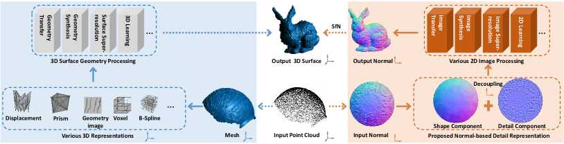
Figure 1: Illustration of the difference of surface geometry detail processing between the traditional 3D representations and the proposed 2D normal-based detail representation. Our method manipulates the 3D surface details in 2D normal domain, which aims to decouple a surface normal map into a shape component and detail component. We theoretically derive that the proposed detail component has the properties of separability, transferability, and idempotence.

Recently, deep learning has achieved a remarkable success in various computer vision tasks [12, 13, 14], which has also been employed for geometry detail processing. For instance, for surface detail transfer, the mapping mechanism between geometric texture and 3D shape can be trained in an end-to-end manner by convolutional neural network (CNN) [15]. For geometry texture synthesis, metric learning can synthesize the small fragment of a given geometry texture on the entire target surface [16]. However, there is still a large room for performance improvement on learning-based geometry detail processing. On one hand, an internal network architecture is usually difficult to be clearly interpretable, and thus the robustness and generalization of learned models cannot be guaranteed for new data samples. On the other, a deep-learned model is usually complicated, and requires a high computation cost.

To overcome the above limitations, the normal vector of a surface shape has been used as the carrier of geometric details. According to the photometry principle [17], the diversity of a surface normal vector contains fine-grained differences in terms of illumination intensities, which is perceived as texture (or geometry details) by human eyes. Besides, the normal map of a 3D surface also conveys a global shape geometry, as demonstrated in [18, 19]. Therefore, a surface normal map encodes both the global shape and the local geometry structure simultaneously.

Inspired by the above discussions, we present a new simple and interpretable framework for geometric detail processing in normal domain. One of the key advantages is that the heavy payload of meshing can he avoided, and the legacy image processing algorithms can be re-used. Unlike those existing approaches, our method rarely relies on the mesh environment. For instance, it can accept real and dense normal data obtained from a real-world surface by photometric stereo [20, 21, 22]. More importantly, we excavate an effective geometry detail representation which allows to be easily processed as a digital image. This is of significant importance for many popular applications in 3D scenarios, due to the fact that most of them have dense and complex micro geometry structures. In addition, surface in the mesh format can be considered as a special case of the proposed framework by recording the patch orientation vectors into a dense normal map which can be easily achieved via MeshLab (see a dense laser-scanning point cloud data in Section 5). The proposed normal-based detail representation is highly effective for surface geometry processing (e.g., geometric texture synthesis, geometry detail transfer, 3D surface super-resolution, etc.), which can be implemented in a light-weight image processing manner as illustrated in Fig. 1.

We highlight our contributions as follows:

• Based on the characteristics of a surface normal representation, we propose to manipulate surface geometry details by excavating the corresponding surface normal into two descriptors: surface shape and geometry detail. As far as we know, this is an earlier exploration to comprehensively manipulate 3D surface detail in a light-weight image processing manner.

• To better analyze the geometry detail descriptor, we further derive and demonstrate three important properties, including detail separability, detail transferability, and detail idempotence. These properties mathematically guarantee that the geometry detail of a source surface can be used as a standalone feature applied to a target shape.

• Based on the proposed normal-based representations, we further design three new schemes for geometric surface detail processing, including geometric texture synthesis, geometry detail transfer, and 3D surface super-resolution. In addition, recent deep-learned models can be seamlessly embedded into the proposed framework. Experiments on the benchmark dataset verify the effectiveness and versatility of our approach over recent competing schemes in terms of both the computing time and memory spaces.

The remainder of this article is organized as follows. Section 2 gives a concise background introduction for recent advances in surface geometry processing. Section 3 presents the geometric surface representation in the normal domain. In Section 4, we describe three main properties of the proposed geometric processing framework, including detail separability, detail transferability, and detail idempotence. Section 5 demonstrates the significant theoretical and practical contributions of this normal-based surface detail representation, and Section 6 provides a discussion for the characteristics of the proposed scheme. Finally, the overall conclusion is drawn in Section 7, and some open ideas are presented to address several remaining challenges for our normal-based geometry processing.

2 Background

For simplicity, we briefly introduce the recent developments of geometry detail processing schemes based on the following four questionable aspects: 1) which domain is the texture pattern defined? 2) whether does it require parameterization? 3) how is the capability in dealing with dense data (measured in patch or pixel)? 4) how is the computational complexity (measured in memory or time)? In general, the first three factors determine the last one. In Table I, we summarize an overall comparison for recent representative methods in surface geometry detail processing.

The proposed method takes a normal map as the input, indicating that it can accept a high-resolution two-dimensional data format. In other words, our method can process a highly-dense geometry texture as a digital image. In addition, the input normal can contain real-world and non-repetitive surface textures, and thus the proposed method is an effective detail representation of surface geometry. Moreover, the normal manipulation does not require a parameterization or mesh environment.

Vertex Displacement-based. The most straightforward way to process geometry details is to represent the texture pattern as a vertex displacement between the target shape and the original surface [1]. This kind of method is too strict and requires more accurate alignment between the target and the original surface [23, 24]. As a result, mesh refinement has to be added to improve the vertex displacement by providing finer texture patterns, examples of which include multi-resolution mesh [25], Laplacian mesh [26], or statistical mesh [27]. However, the mesh refinement heavily depends on the parameterization, which degrades its applicability.

TABLE I: Comparisons of the representative schemes for 3D surface geometry detail processing.

Method Domain Parameterization Density Complexity [1] Mesh Yes Patch/pixel Medium [23] Mesh Yes Patch/pixel Medium [25] Mesh Yes Patch High [28] Mesh Yes Patch Medium [26] Mesh Yes Patch High [29] B-spline Yes Patch High [30] Wavelet Yes Patch Medium [31] Prism Yes Patch High [8] Voxel Yes Patch High [32] Geometry image Yes Patch/pixel Medium [15] Mesh No Patch Medium [16] Mesh No Patch Medium Proposed Normal No Patch/pixel Low

Domain-guided. It was once popular to transfer the texture information to another domain for effective processing. Due to the implicit expression in texture description, B-spline curve [29] has been employed to fit both the source and target surface, but the parameter-tuning of the B-spline curve for a complex surface is another major challenge. In the earliest domain-guided approaches, the source surface and target shape have been also transferred to the frequency domain [30] to separate the details and shape as a high-frequency and low-frequency coefficient, respectively. Recently, some new representations have been used to process surface details, such as displacement volume [31], voxel-based [8], and geometry image [32]. Although some complex and non-repeating texture patterns can be accurately addressed, the massive computation for auxiliary vertexes or surface re-meshing makes them difficult to be extended in dealing with dense surfaces.

Data-driven. Surface editing of the source texture to the target shape can be considered as a mapping process. Data-driven approaches [15, 16] have recently been leveraged to directly learn the mapping between the source and the target, as such that a geometry texture pattern can be automatically synthesized and transferred. This kind of method can effectively avoid the parameterization and the definition of textures. However, at present, they are difficult to be interpretable, and require very high computing resources.

Undoubtedly, the data-driven framework will be one of the main streams to solve 3D problems in future, but currently it is not universal, especially when high-dimensional geometric features are involved. If a geometry detail representation can be dimensionally reduced to the 2D pixel domain, various well developed image-based learning networks can be leveraged to solve existing 3D surface processing problems. This intuitive idea directly inspires this work.

3 Geometric Surface Representation in Normal Domain

Normal Map Definition. A normal map $\mathcal{N}\in\mathbb{R}^{3\times H\times W}$ (e.g., 3 channels, height $H$, and width $W$) is such an image that can be obtained by virtual or real imaging projection of a target surface under a single view. The normal map $\mathcal{N}$ has three channels, where each normal pixel represents a normalized normal vector (i.e., xyz components) on its corresponding surface point. Now let us backproject $\mathcal{N}$ onto its 3D surface and consider it in the 3D discrete settings. Specifically, for a 3D surface, it can be regarded as composed of numerous small patches (or facets) [33, 34]. Globally, every patch has a specific orientation, and is connected with each other to form a 3D shape. At the same time, the orientation difference among adjacent patches causes a local surface roughness, i.e., micro geometric structures. The orientation of each surface patch is projected onto the viewing plane to obtain the corresponding normal vector. Thus, a normal map simultaneously encodes both the global shape and the local geometry detail (or micro structure/texture) of its projected surface.

Normal Map Generation. For photometric stereo, the normal of a 3D surface point corresponding to the normal pixel can be calculated from the pixel magnitude of multiple images according to the principle of Lambertian reflection [21, 22]. For a 3D mesh or point clouds, the normal map can be generated through orthographic or perspective projection of a virtual camera. It is noted that our method is independent of normal map generation from orthographic and perspective projections. For a normal map generated from photometric stereo, the practical imaging process is under the perspective projection. For a normal map generated from point cloud data, we choose the orthographic projection to facilitate the calculation process. Specifically, at a fixed view angle, visible surface points will be projected onto a virtual image plane, and then their normal vectors will be recorded on the corresponding pixel coordinates to form a normal map, where the normal vector is a fitted local surface orientation of all points in a small region. A detailed description of normal map estimation for point clouds is referred to here. Therefore, the generation of normal maps is as convenient as taking photographs, but they have the same constraints of single-view imaging.

Based on the observation that, by increasing the diversity of normal orientations while keeping their original low-frequency components, the geometry surface details can be enriched without distorting its global shape, and we come up with a new extraction method for geometry details from a surface normal map, and show its high transferability to another surface with different shapes. In the rest of this section, we show the possibility of excavating these two feature representations (i.e., global shape and local geometry details) from a single normal map, and give their mathematical expressions.

Specifically, a given normal map $\mathcal{N}$ is used to obtain a shape component and a detail component, where the shape component and the detail component are calculated by Eq. (1) in Section 3.1 and Eq. (2) in Section 3.2, respectively. Geometrically, the relationship between $\mathcal{N}$ and its shape component and the detail component can be also illustrated as the transformation process between the global coordinate system (left) and the local coordinate system (right), as shown in Fig. 2.

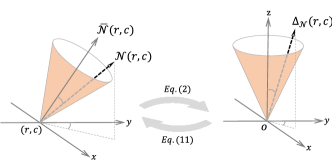
Figure 2: Illustration of the relative coordinate transformation for extracting the detail component representation in Section 3.2.

3.1 Surface Shape Representation

After removing the fine-grained texture structure from an object surface, the result of smoothing can be considered to only convey shape information [35, 36]. To derive the surface smoothing operation in the normal domain, we observe that a surface roughness decreases as the variance of the local neighborhood normals decreases. Consequently, if there is a way to reduce the local variance, a global surface shape can be obtained based on its normal map. In view of this, we adopt the smoothing operation as a low-pass filter on the normal map $\mathcal{N}$.

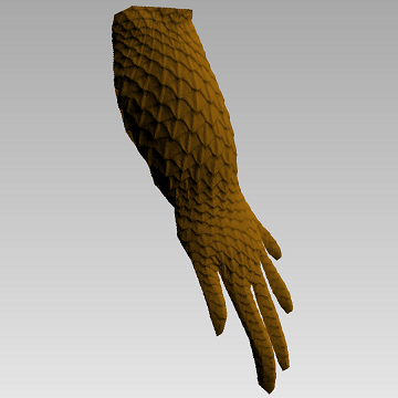
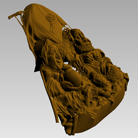
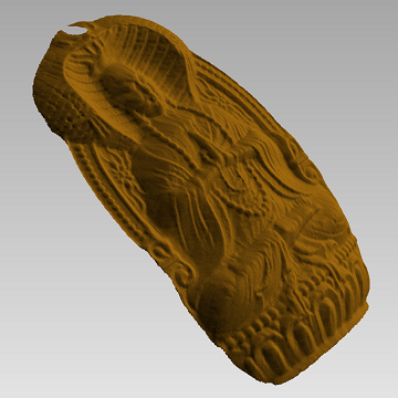
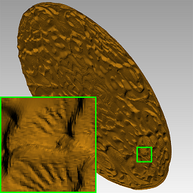
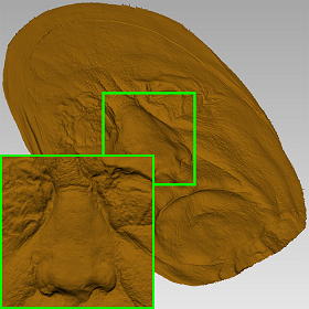
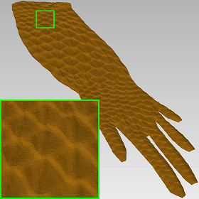
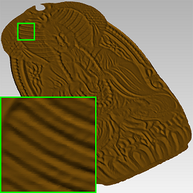
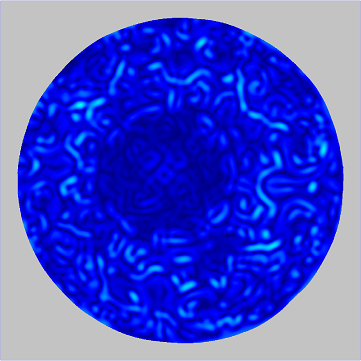
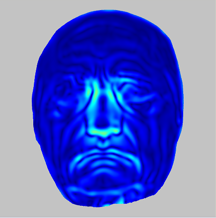
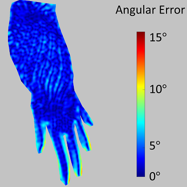
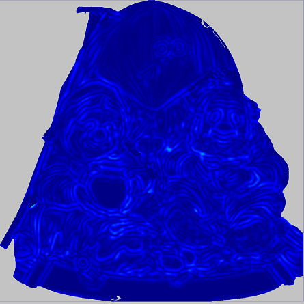
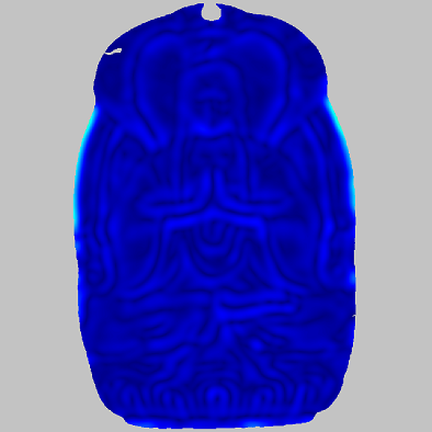
Circular ($0.96^{\circ}$)	Geothe ($0.95^{\circ}$)	Lizard ($1.47^{\circ}$)	Panno ($0.44^{\circ}$)	Woodcarving ($0.47^{\circ}$)

Figure 3: Property of the extracted detail component representation. The top row shows five five different 3D models, the middle row shows the reconstructed surface of the corresponding shape component, and the bottom row shows the error map $E_{mae}$ between $\bar{\Delta}_{\mathcal{N}}$ and $\mathbf{z}$. The reconstructed surfaces of the detail component maps are flatten and oriented towards the $z$-axis, which is shape-uncorrelative to the original surface.

For a surface with the normal map $\mathcal{N}$, its surface shape in the normal domain is represented as $\bar{\mathcal{N}}$ and formulated by Eq. (1).

$$\small\bar{\mathcal{N}}\left({r,c}\right)=Conv\left(\mathcal{N},\kappa\right),$$ (1)

where $\kappa$ denotes a $(2w+1)$ by $(2w+1)$ Gaussian or average convolution kernel, $w$ is set to $5$ or $7$ in the experiments, and $Conv(\cdot)$ represents the convolution operation.

It is noted that all the discussed normal vectors are normalized below, and can be represented on a unit sphere. $\bar{\mathcal{N}}\left({r,c}\right)\in\mathbb{R}^{3}$ in Eq. (1) can be visualized as the center of a solid angle $\eta(r,c)$, which is a subset of normals in a $(2w+1)$$\times$$(2w+1)$ window, i.e., $\eta(r,c)=\left\{{\mathcal{N}\left({s,t}\right)\left|{r-w\leq s\leq r+w;c-w\leq t\leq t+w}\right.}\right\}$. Apparently, the smoother the normal map $\mathcal{N}$, the smaller the variance of the normals in $\eta(\cdot)$, and the closer $\mathcal{N}(r,c)$ to the center of $\eta(\cdot)$. In turn, it can be considered that $\bar{\mathcal{N}}$ represents the pure shape of $\mathcal{N}$. Therefore, $\bar{\mathcal{N}}$ in Eq. (1) is also called shape component, and $\bar{\mathcal{N}}\left({r,c}\right)$ is supposed to be similar to each other within a small $(2w+1)$$\times$$(2w+1)$ window.

3.2 Geometry Detail Representation

Intuitively, the difference between a normal map and its shape component determines the roughness of an input surface. This phenomenon has been verified in [2, 37, 38], where a normal map can be sharpened by increasing the angle between $\mathcal{N}$ and $\bar{\mathcal{N}}$. In this section, we use this clue to define detail component in terms of normals.

Ideally, the detail component feature is expected to contain no shape information. In other words, it should be only related texture or micro structure, and should not exhibit concrete shapes compared to the shape component extracted from a surface. Meanwhile, the detail component should keep high similarity with the local original surface, as the detail feature can be well represented. Although the direct subtraction of $\mathcal{N}$ and $\bar{\mathcal{N}}$ can describe this subtle difference, it will be over strict when used to measure the practical geometry details. Therefore, how to derive a detail-without-shape feature is our focus.

Let us consider a normal vector $\mathcal{N}(r,c)$ and its shape component $\bar{\mathcal{N}}\left({r,c}\right)$ as given in Fig. 2 (left), in which our interests are primarily focused on their relative differences. A reasonable way to describe such a relative difference is to transform them into a relative coordinate system, under which, the mapping of $\mathcal{N}(r,c)$ can represent this difference as illustrated in Fig. 2 (right). By comparing these two coordinate systems in Fig. 2, it is not difficult to find that such a relative coordinate system takes the mapping of $\bar{\mathcal{N}}\left({r,c}\right)$ as its $z$-axis. To this end, we define the detail component along with the relative coordinate transformation as follows.

For a given $\mathcal{N}(r,c)$ and its shape component $\bar{\mathcal{N}}(r,c)$, the corresponding detail component ${\Delta_{\mathcal{N}}}\left({r,c}\right)$ can be computed as the mapping of $\mathcal{N}(r,c)$ in the relative coordinate system whose $z$-axis is the mapping of $\bar{\mathcal{N}}(r,c)$.

$${\Delta_{\mathcal{N}}}\left({r,c}\right)=\mathbf{R}\left|{{}_{\bar{\mathcal{N}}\left({r,c}\right),\mathbf{z}}}\right.\cdot\mathcal{N}\left({r,c}\right),$$ (2)

where $\cdot$ denotes the multiplication operator of matrix and vector, $\mathcal{N}(r,c)$ is a 3$\times$1 column vector, and $\mathbf{R}\left|{{}_{\bar{\mathcal{N}}\left({r,c}\right),\mathbf{z}}}\right.$ represents a 3$\times$3 rotation matrix that can transform vector $\bar{\mathcal{N}}\left({r,c}\right)$ to the vector $\mathbf{z}=[0,0,1]^{T}$, i.e.,

$$\mathbf{z}=\mathbf{R}\left|{{}_{\bar{\mathcal{N}}\left({r,c}\right),\mathbf{z}}}\right.\cdot{\bar{\mathcal{N}}\left({r,c}\right)}.$$ (3)

According to Rodrigues’ rotation formula [39], $\mathbf{R}\left|{{}_{\bar{\mathcal{N}}\left({r,c}\right),\mathbf{z}}}\right.$ can be determined from $\bar{\mathcal{N}}(r,c)$ and $\mathbf{z}$ as

$$\small\mathbf{R}\left|{{}_{{\bar{\mathcal{N}}}\left({r,c}\right),\mathbf{z}}}\right.=\mathbf{I}+{\left\lfloor{{\bar{\mathcal{N}}}\left({r,c}\right)\otimes\mathbf{z}}\right\rfloor_{\times}}+\frac{{\left\lfloor{{\bar{\mathcal{N}}}\left({r,c}\right)\otimes\mathbf{z}}\right\rfloor_{\times}^{2}}}{{1+{\bar{\mathcal{N}}}\left({r,c}\right)\odot\mathbf{z}}},$$ (4)

where $\otimes$ denotes the cross product operator, $\odot$ represents the dot product operator, $\mathbf{I}\in\mathbb{R}^{3\times 3}$ denotes the identity matrix, and $\left\lfloor{\mathbf{v}}\right\rfloor_{\times}$ represents the skew-symmetric cross-product matrix of vector $\mathbf{v}$. Finally, we obtain the expression of $\mathbf{R}\left|{{}_{\bar{\mathcal{N}}\left({r,c}\right),\mathbf{z}}}\right.$ as,

$$\mathbf{R}\left|{{}_{\bar{\mathcal{N}}\left({r,c}\right),\mathbf{z}}}\right.=\begin{bmatrix}1-\frac{\bar{n}_{x}^{2}}{1+\bar{n}_{z}}&-\frac{\bar{n}_{x}\bar{n}_{y}}{1+\bar{n}_{z}}&-\bar{n}_{x}\\ -\frac{\bar{n}_{x}\bar{n}_{y}}{1+\bar{n}_{z}}&1-\frac{\bar{n}_{y}^{2}}{1+\bar{n}_{z}}&-\bar{n}_{y}\\ \bar{n}_{x}&\bar{n}_{y}&1-\frac{\bar{n}_{x}^{2}+\bar{n}_{y}^{2}}{1+\bar{n}_{z}}\end{bmatrix},$$ (5)

where $\bar{n}_{x}$, $\bar{n}_{y}$ and $\bar{n}_{z}$ are the $xyz$ components of ${\bar{\mathcal{N}}}\left({r,c}\right)$.

Fig. 3 shows five representative 3D models and the relevant detail component results. It is noted that, to visualize the detail component, we obtain their depth values via the surface from normals (SfN) method in [19]. In addition, we also measure the shape of $\Delta_{\mathcal{N}}$, where the energy map of angular error between $\bar{\Delta}_{\mathcal{N}}$ and $\mathbf{z}$ is calculated. Moreover, we calculate the structure similarity (SSIM) metric [40] between the extracted detail component by Eq. (2) and its original normal map. From left to right, the relevant $\mathbf{E}_{ssim}$ scores are 0.9566, 0.9531, 0.9882, 0.9557, and 0.9737, respectively. As expected, all the extracted detail component is detail-without-shape and appears to be unwrapped and flattened.

4 Properties of the Detail Component

The detail component is not just an unwrapped surface as it looks. To better analyze the characteristics of the detail component, we demonstrate three important properties and provide the related mathematical derivations as follows.

4.1 Detail Separability

According to the detail component extracted by Eq. (2), we find that the shape of an detail component is a flatten surface and oriented towards the $z$-axis. In other words, the detail component contains no shape information compared to the source 3D surface. This property of the detail component is named as detail separability. We give a detailed explanation as follows.

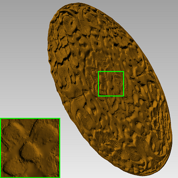
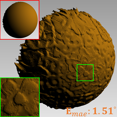
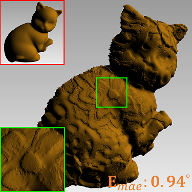
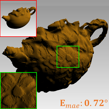
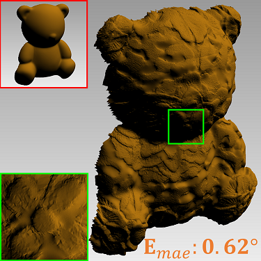
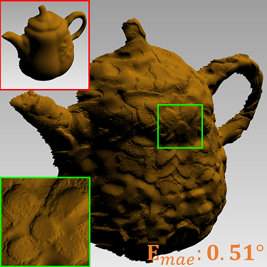
Original details	Ball	Cat	Pot1	Bear	Pot2
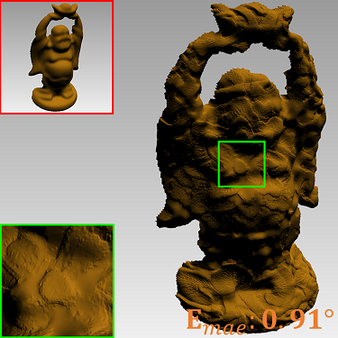
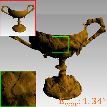
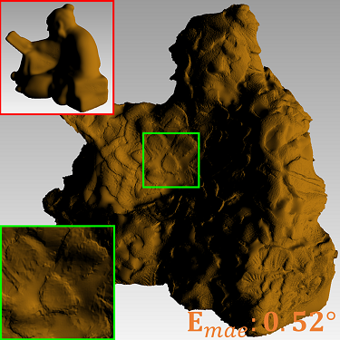
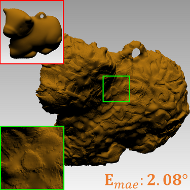
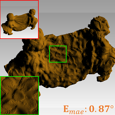
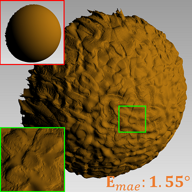
Buddha	Goblet	Reading	Cow	Harvest	∗Ball

Figure 4: Illustration of the detail transferability property for the proposed detail component. The geometry details of Circular is transferred one after another on 10 different models from DiLiGenT [41] and finally transferred back to the first model (^∗Ball). The shape difference (in terms of mean angular error (MAE)) is provided at the bottom of each target object, which is calculated between the current shape before detail transfer and the extracted shape after detail transfer.

According to the shape component definition in Eq. (1), $\bar{\mathcal{N}}(r,c)$ can be represented by

$$\small\bar{\mathcal{N}}\left({r,c}\right)={\lambda_{1}}\sum\limits_{s=-w}^{w}{\sum\limits_{t=-w}^{w}{\kappa\left({s,t}\right)\mathcal{N}\left({r+s,c+t}\right)}},$$ (6)

where according to Eq. (3), $\bar{\mathcal{N}}(r,c)$ can be calculated from $\mathbf{z}$, like $\bar{\mathcal{N}}\left({r,c}\right)={\left({\mathbf{R}\left|{{}_{\bar{\mathcal{N}}\left({r,c}\right),{\mathbf{z}}}}\right.}\right)^{-1}}{\cdot{\mathbf{z}}}$, and according to Eq. (2), ${\mathcal{N}}(r,c)$ can be calculated from $\Delta_{\mathcal{N}}(r,c)$, like $\mathcal{N}\left({r+s,c+t}\right)={\left({\mathbf{R}\left|{{}_{\bar{\mathcal{N}}\left({r+s,c+t}\right),{\mathbf{z}}}}\right.}\right)^{-1}}\cdot{\Delta_{\mathcal{N}}}\left({r+s,c+t}\right)$. It is noted that to simplify the expression, $\lambda_{1}$ represents a normalization constant to ensure that the filtered normals have unit length.

By submitting them into Eq. (6), we have

$$\small\begin{split}&\left({{{\left({\mathbf{R}\left|{{}_{\bar{\mathcal{N}}\left({r,c}\right),{\mathbf{z}}}}\right.}\right)}^{-1}}\cdot{\mathbf{z}}}\right)={\lambda_{1}}\\ &\leavevmode\resizebox{422.77661pt}{}{$\sum\limits_{s=-w}^{w}{\sum\limits_{t=-w}^{w}{\kappa\left({s,t}\right)\left[{{{\left({\mathbf{R}\left|{{}_{\bar{\mathcal{N}}\left({r+s,c+t}\right),{\mathbf{z}}}}\right.}\right)}^{-1}}\cdot{\Delta_{\mathcal{N}}}\left({r+s,c+t}\right)}\right]}}$},\end{split}$$ (7)

For a dense surface, its shape component is assumed to be continuous and change slowly within a small surface patch (the related proof can be found in [42], 11$\times$11), and their corresponding rotation matrices ${\mathbf{R}\left|{{}_{\bar{\mathcal{N}}\left({r+s,c+t}\right),\mathbf{z}}}\right.}$ should be similar. To verify this condition, we calculate the average rotation angle between $\left.\mathbf{R}\right|_{\bar{\mathcal{N}}\left({r,c}\right),\mathbf{z}}$ and ${\left.\mathbf{R}\right|_{\bar{\mathcal{N}}\left({r+s,c+t}\right),\mathbf{z}}}$ as formulated in Eq. (8).

$$\small\bar{\theta}\left({r,c}\right)=\frac{1}{{{{\left({2w+1}\right)}^{2}}}}\sum\limits_{s=-w}^{w}{\sum\limits_{t=-w}^{w}{\theta\left({s,t}\right)}},$$ (8)

where $\theta\left(\cdot\right)$ is calculated by

$$\small\leavevmode\resizebox{446.2658pt}{}{$\theta\left({r,c}\right)=arccos\left({{{\left({trace\left({\left.\mathbf{R}\right|_{\bar{\mathcal{N}}\left({r,c}\right),\mathbf{z}}\cdot\left({\left.\mathbf{R}\right|_{\bar{\mathcal{N}}\left({r+s,c+t}\right),\mathbf{z}}}\right)^{T}}\right)-1}\right)}\mathord{\left/{\vphantom{{\left({trace\left({\left.\mathbf{R}\right|_{\bar{\mathcal{N}}\left({r,c}\right),z}\left({\left.\mathbf{R}\right|_{\bar{\mathcal{N}}\left({r+s,c+t}\right),\mathbf{z}}}\right)^{T}}\right)-1}\right)}2}}\right.\kern-1.2pt}2}}\right)$},$$

where $T$ represents the transpose of a matrix. Apparently, the closer $\bar{\theta}$ to $0$, the more similar in ${\mathbf{R}\left|{{}_{\bar{\mathcal{N}}\left({r+s,c+t}\right),\mathbf{z}}}\right.}$.

Moreover, we provide three different norms to measure the distance between ${{{\mathbf{R}}\left|{{}_{\bar{\mathcal{N}}\left({r,c}\right),{\mathbf{z}}}}\right.}\cdot{{\left({{\mathbf{R}}\left|{{}_{\bar{\mathcal{N}}\left({r+s,c+t}\right),{\mathbf{z}}}}\right.}\right)}^{-1}}}$ and the identity matrix ${\mathbf{I}}$:

$$\begin{split}{\bar{\mathcal{\ell}}_{p}}\left({r,c}\right)=&\leavevmode\resizebox{347.62126pt}{}{$\frac{1}{{{{\left({2w+1}\right)}^{2}}}}{\sum\limits_{s=-w}^{w}{\sum\limits_{t=-w}^{w}{{{\left\|{\left({{\mathbf{R}}\left|{{}_{\bar{\mathcal{N}}\left({r,c}\right),{\mathbf{z}}}}\right.}\right)\cdot{{\left({{\mathbf{R}}\left|{{}_{\bar{\mathcal{N}}\left({r+s,c+t}\right),{\mathbf{z}}}}\right.}\right)}^{-1}}-{\mathbf{I}}}\right\|}_{p}}}}}$},\\ &p=1,2,or,\infty,\end{split}$$

Table II provides the results of five representative 3D objects in terms of the average rotation angle $\bar{\theta}$ and the average value of three norms ${\bar{\mathcal{\ell}}_{p}}$. As seen, all of these metrics have small values. For example, the average rotation angles are less than $0.61^{\circ}$, and the largest norm value is less than $0.014$.

TABLE II: Property of the shape component in terms of the rotation angle and the matrix norm.

	Circular	Goethe	Lizard	Panno	Woodcarving
$\bar{\theta}$	$0.4950^{\circ}$	$0.6049^{\circ}$	$0.3249^{\circ}$	$0.3391^{\circ}$	$0.4678^{\circ}$
${\bar{\ell}_{1}}$	0.0109	0.0133	0.0066	0.0074	0.0100
${\bar{\ell}_{2}}$	0.0086	0.0106	0.0057	0.0059	0.0082
${\bar{\ell}_{\infty}}$	0.0109	0.0133	0.0066	0.0074	0.0100

As a result, every $\mathbf{R}\left|{{}_{\bar{\mathcal{N}}\left({r+s,c+t}\right),\mathbf{z}}}\right.$ can be approximately replaced by $\mathbf{R}\left|{{}_{\bar{\mathcal{N}}\left({r,c}\right),\mathbf{z}}}\right.$, and Eq. (7) can be rewritten as

$$\small\begin{split}&\left({{{\left({\mathbf{R}\left|{{}_{\bar{\mathcal{N}}\left({r,c}\right),{\mathbf{z}}}}\right.}\right)}^{-1}}\cdot{\mathbf{z}}}\right)\\ &\leavevmode\resizebox{422.77661pt}{}{${\approx{\lambda_{1}}\sum\limits_{s=-w}^{w}{\sum\limits_{t=-w}^{w}{\kappa\left({s,t}\right)\left[{{{\left({\mathbf{R}\left|{{}_{\bar{\mathcal{N}}\left({r,c}\right),{\mathbf{z}}}}\right.}\right)}^{-1}}\cdot{\Delta_{\mathcal{N}}}\left({r+s,c+t}\right)}\right]}}}$}\\ &{={\lambda_{1}}{{\left({\mathbf{R}\left|{{}_{\bar{\mathcal{N}}\left({r,c}\right),{\mathbf{z}}}}\right.}\right)}^{-1}}\cdot\sum\limits_{s=-w}^{w}{\sum\limits_{t=-w}^{w}{\kappa\left({s,t}\right){\Delta_{\mathcal{N}}}\left({r+s,c+t}\right)}}},\end{split}$$ (9)

where the right side is actually the shape component representation of ${\Delta_{\mathcal{N}}}\left({r,c}\right)$ according to Eq. (6). Finally, when multiplying ${\mathbf{R}\left|{{}_{{\bar{\mathcal{N}}}\left({r,c}\right),\mathbf{z}}}\right.}$ on both side of Eq. (9), we have

$$\mathbf{z}{\approx}{{\bar{\Delta}}_{\mathcal{N}}}\left({r,c}\right).$$ (10)

Eq. (10) reveals that the shape of ${\Delta_{\mathcal{N}}}$ is a flat surface, and oriented towards the $z$-axis. Moreover, it is shape-uncorrelative to the original surface. Thus, the detail separability property has been demonstrated. Fig. 3 provides five representative 3D models from simple repeating patterns to complex textures. In the second row, the reconstructed surfaces from all five extracted detail component maps are oriented towards the $z$-axis, which are consistent with the deduction in Eq. (10).

4.2 Detail Transferability

The significance of the proposed detail component representation lies in the fact that it can be extracted as separable features used for 3D surface editing, in which the texture transferability to another surface is an essential goal. According to Eq. (2), a surface normal $\mathcal{N}\left({r,c}\right)$ can be computed from its shape component $\bar{\mathcal{N}}(r,c)$ and the detail component $\Delta_{\mathcal{N}}(r,c)$,

$$\small\begin{split}{\mathcal{N}}\left({r,c}\right)&=({\mathbf{R}}\left|{{}_{{\bar{\mathcal{N}}}\left({r,c}\right),\mathbf{z}}}\right.)^{-1}\cdot{\Delta_{\mathcal{N}}}\left({r,c}\right)\\ &={\mathbf{R}}\left|{{}_{{\mathbf{z},\bar{\mathcal{N}}}\left({r,c}\right)}}\right.\cdot{\Delta_{\mathcal{N}}}\left({r,c}\right).\end{split}$$ (11)

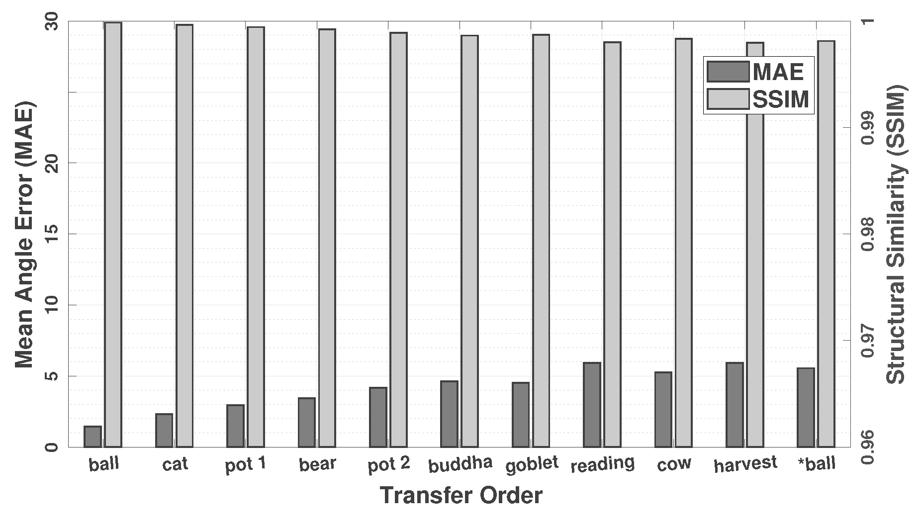
Figure 5: The mean angular error (MAE) and structural similarity (SSIM) results of Circular. The reported MAE and SSIM results are obtained by transferring one after another on $10$ different models.

Considering the detail separability property, ${\Delta_{\mathcal{N}(r,c)}}$ contains no concrete shape information (i.e., a flat plane), which implies that $\bar{\mathcal{N}}(r,c)$ can be replaced with an arbitrarily target shape. In Eq. (11), replacing $\bar{\mathcal{N}}(r,c)$ with another surface while keeping ${\Delta_{\mathcal{N}(r,c)}}$ unchanged is named as detail transferability. We demonstrate the detail transferability property, and provide the related mathematical proofs as follows.

Let the detail component ${\Delta_{{{\mathcal{N}}_{org}}}}$ be separated from a source normal map $\mathcal{N}_{org}$, and assume that it can be transferred to a target surface with the normal map ${\bar{\mathcal{N}}_{tgt}}$ via

$${{\mathcal{N}}^{*}}\left({r,c}\right)=\mathbf{R}\left|{{}_{\mathbf{z},{{{\bar{\mathcal{N}}}}_{tgt}}\left({r,c}\right)}}\right.\cdot{\Delta_{{{\mathcal{N}}_{org}}}}\left({r,c}\right).$$ (12)

For a successful geometry detail transfer, $\mathcal{N}^{*}$ is expected to have the similar surface shape as that of ${\bar{\mathcal{N}}_{tgt}}$ as well as the similar geometry details as that of $\mathcal{N}_{org}$. In the following section, we demonstrate that both of them can be guaranteed based on the proposed normal-based framework.

Shape similarity: According to Eq. (6), the shape component of ${{\mathcal{N}}^{*}}\left({r,c}\right)$ can be represented by

$$\small{\bar{\mathcal{N}}^{*}}\left({r,c}\right)={\lambda_{2}}\sum\limits_{s=-w}^{w}{\sum\limits_{t=-w}^{w}{\kappa\left({s,t}\right){\mathcal{N}^{*}}\left({r+s,c+t}\right)}},$$ (13)

where $\lambda_{2}$ represents a normalization constant to ensure that the filtered normals have unit length.

For a smooth $\bar{\mathcal{N}}_{tgt}$ (with the shape information only), $\{\mathbf{R}\mid_{\mathbf{z},\mathcal{N}_{tgt}(r+s,c+t)}\}$ is highly similar to each other within a small $(2w+1)$$\times$$(2w+1)$ window, as demonstrated in Section 4.1. Moreover, by submitting $\mathcal{N}^{*}(r,c)$ into Eq. (13), it has the following approximated expression,

$$\small\begin{split}&{{\bar{\mathcal{N}}}^{*}}\left({r,c}\right)\approx\\ &\leavevmode\resizebox{413.38667pt}{}{${\lambda_{2}}\mathbf{R}\left|{{}_{{\mathbf{z}},{{\bar{\mathcal{N}}}_{tgt}}\left({r,c}\right)}}\right.\cdot\sum\limits_{s=-w}^{w}{\sum\limits_{t=-w}^{w}{\kappa\left({s,t}\right){\Delta_{{\mathcal{N}_{org}}}}\left({r+s,c+t}\right)}}$}.\end{split}$$ (14)

According to the detail separability property, the sum of $\Delta_{\mathcal{N}_{org}}(r,c)$ in a small window is approximately parallel to $z$-axis. Thus, Eq. (14) can be simplified as

$$\small\begin{split}\bar{\mathcal{N}}^{*}(r,c)&\approx\mathbf{R}\mid_{\mathbf{z},{\bar{\mathcal{N}}}_{tgt}(r,c)}\cdot~{}~{}\mathbf{z}\\ &={\bar{\mathcal{N}}_{tgt}}\left({r,c}\right).\end{split}$$ (15)

Consequently, this indicates that the transferred result, $\mathcal{N}^{*}$, has the similar shape as the target surface $\bar{\mathcal{N}}_{tgt}$. Fig. 4 shows the detail transferability property on the DiLiGenT dataset [41]. The detail component of the Circular model from Aim@Shape is used as the source ${\Delta_{{{\mathcal{N}}_{org}}}}\left({r,c}\right)$, and the shape components of all 3D models from the DiLiGenT are used as the target ${\bar{\mathcal{N}}_{tgt}}\left({r,c}\right)$. The widely-used mean angular error (MAE) [19, 43] is also adopted to measure the reconstructed shape similarity. In Fig. 4, the numeric values are calculated between the target shape before detail transfer and the extracted shape after detail transfer. For instance, the $E_{mae}$ value of Bear represents the shape difference between before and after detail transfer from Pot1. The maximum $\mathbf{E}_{mae}$ value is $2.08^{\circ}$, which indicates a very promising shape similarity. The visual results are consistent with the MAE results.

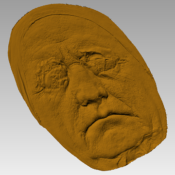
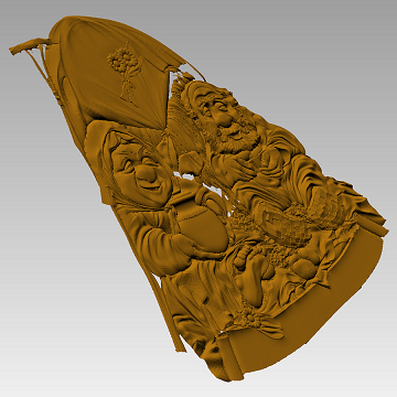
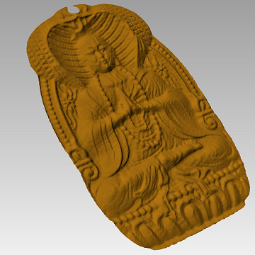
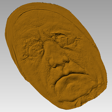
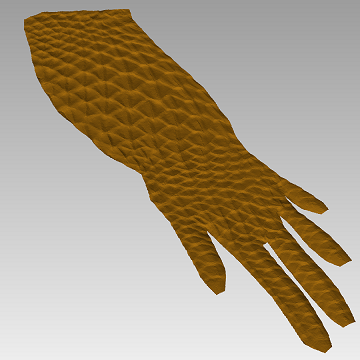
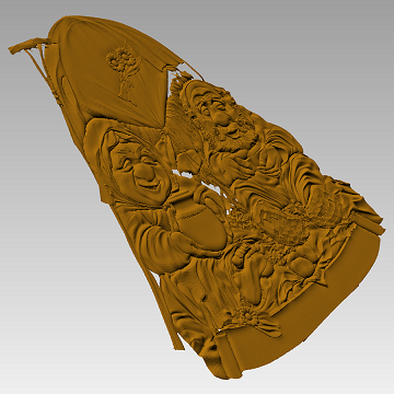
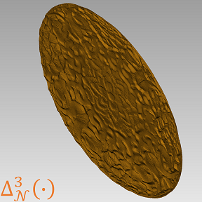
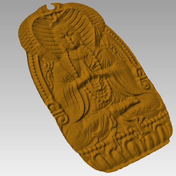
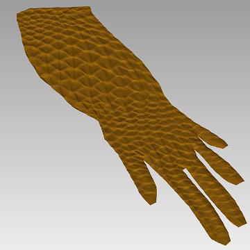
Circular	Geothe	Lizard	Panno	Woodcarving

Figure 6: Illustration of the detail idempotence property for the detail component. From the top row to the bottom row: ${\Delta_{\mathcal{N}}}\left(\cdot\right)$, ${\Delta_{\mathcal{N}}^{2}}\left(\cdot\right)$, ${\Delta_{\mathcal{N}}^{3}}\left(\cdot\right)$, and ${\Delta_{\mathcal{N}}^{4}}\left(\cdot\right)$.

Detail similarity: The detail component of $\mathcal{N}^{*}$ can be calculated by Eq. (2) as

$$\small{\Delta_{{{\mathcal{N}}^{*}}}}\left({r,c}\right)=\mathbf{R}\left|{{}_{{{{\bar{\mathcal{N}}}}^{*}}\left({r,c}\right),\mathbf{z}}}\right.\cdot{{\mathcal{N}}^{*}}\left({r,c}\right).$$ (16)

By submitting Eq. (15) and Eq. (12) into it, we have

$$\small\begin{split}{\Delta_{{{\mathcal{N}}^{*}}}}\left({r,c}\right)&\approx\mathbf{R}\left|{{}_{{{{\bar{\mathcal{N}}}}_{tgt}}\left({r,c}\right),\mathbf{z}}}\right.\cdot\mathbf{R}\left|{{}_{\mathbf{z},{{{\bar{\mathcal{N}}}}_{tgt}}\left({r,c}\right)}}\right.\cdot{\Delta_{{{\mathcal{N}}_{org}}}}\left({r,c}\right)\\ &={\Delta_{{{\mathcal{N}}_{org}}}}\left({r,c}\right).\end{split}$$ (17)

This indicates that the transferred result of $\mathcal{N}^{*}$ has the similar detail as the original surface of $\mathcal{N}_{org}$. Fig. 4 shows the experiments of the detail component transferred on various 3D surface shapes. To evaluate the robustness of detail similarity in Eq. (17), we evaluate the attenuation of the detail component of Circular which is transferred and re-extracted one after another on $10$ different models from the DiLiGenT. For example, the detail component of the Circular is transferred on the first model, i.e., Ball. Then, the new detail component is re-extracted from the transferred result of ball, and it is transferred on the second model, i.e., Cat. Repetitively, this operation is performed on 10 different 3D models, and finally, it is re-transferred on the first model denoted as ^∗Ball.

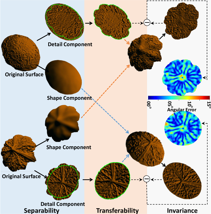
Figure 7: Illustration of the three properties for the detail component. The Circular and Walnut models are used to demonstrate the three properties of the detail component, including separability, transferability, and idempotence as described in Sections 4.1, 4.2, and 4.3, respectively.

In addition, we evaluate the detail similarity of Fig. 4 in terms of both $\mathbf{E}_{ssim}$ and $\mathbf{E}_{mae}$ from the perspective of accumulation transfer error. In Fig. 5, the numeric values are calculated between the transferred detail exacted from the target object and that from the original one. For instance, the $E_{mae}$ value of Bear represents the exacted detail difference between Bear and Ball. The bar-chart in Fig. 5 shows that, with the increase of the transferred times, the detail similarity decays slowly, which is consistent with our cognition. At the same time, the $\mathbf{E}_{ssim}$ values are above $0.9980$, and the $\mathbf{E}_{mae}$ values are below $5^{\circ}$.

4.3 Detail Idempotence

In this section, we demonstrate that the repeatedly extracted detail component is highly similar to the original detail component map, also called detail idempotence.

Taking ${\Delta_{\mathcal{N}}}$ as an independent normal map, its detail component, ${\Delta_{{\Delta_{\mathcal{N}}}}}$, can be further expanded as:

$${\Delta_{\mathcal{N}}^{2}}\left({r,c}\right)\buildrel\Delta\over{=}{\Delta_{{\Delta_{\mathcal{N}}}}}\left({r,c}\right)=\mathbf{R}\left|{{}_{{{\bar{\Delta}}_{\mathcal{N}}}\left({r,c}\right),\mathbf{z}}}\right.\cdot{\Delta_{\mathcal{N}}}\left({r,c}\right),$$ (18)

where ${{{\bar{\Delta}}_{\mathcal{N}}}\left({r,c}\right)}$ can be approximated by $z$, as demonstrated in Section 4.1. Fig. 6 provides the detail component results of the first four orders ${\Delta_{\mathcal{N}}^{k}}\left({r,c}\right),k=1,2,3,4$.

Since $\mathbf{z}=\lambda_{1}\bar{\Delta}_{{\mathcal{N}}}\left({r,c}\right)$, $\mathbf{R}\left|{{}_{{{\bar{\Delta}}_{\mathcal{N}}}\left({r,c}\right),\mathbf{z}}}\right.$ can be approximated as $\mathbf{R}\left|{{}_{\mathbf{z},\mathbf{z}}}\right.$, which is an identity matrix according to Rodrigues’ rotation formula [39]. Therefore, $\mathbf{R}\left|{{}_{{{\bar{\Delta}}_{\mathcal{N}}}\left({r,c}\right),\mathbf{z}}}\right.$ is close to an identity matrix, and Eq. (18) can have a similar form as follows.

$${\Delta_{\mathcal{N}}^{2}}\left({r,c}\right)\approx{\Delta_{\mathcal{N}}}\left({r,c}\right).$$ (19)

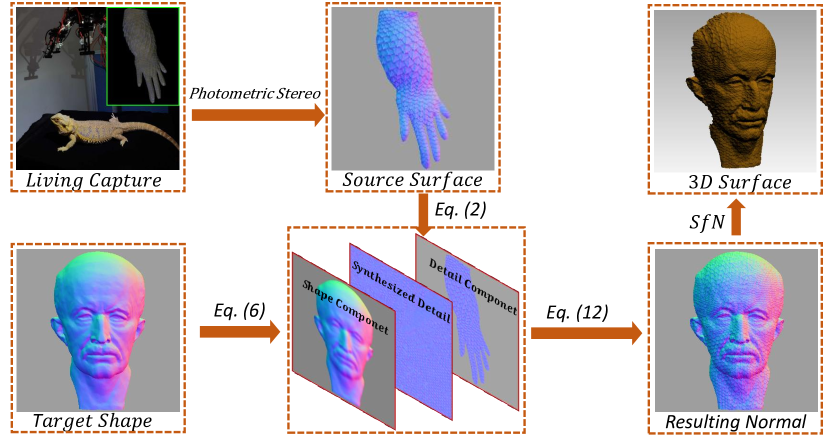
Figure 8: Flowchart of the geometric texture synthesis. The shape component and detail component of the original normal are extracted by Eq. (1) and Eq. (2), respectively. Then, the detail component is synthesized by [44] and transferred to the target normal by Eq. (12). Finally, the target 3D surface is reconstructed by the surface-from-normal (SfN) method [19].

TABLE III: Evaluations of the detail idempotence property between the high order $\Delta_{\mathcal{N}}$ and the corresponding original normal map.

SSIM	Circular	Goethe	Lizard	Panno	Woodcarving
$\left[{{\Delta_{\mathcal{N}}^{2}}\left(\cdot\right),{\Delta_{\mathcal{N}}}\left(\cdot\right)}\right]$	0.9996	0.9988	0.9996	0.9970	0.9982
$\left[{{\Delta_{\mathcal{N}}^{3}}\left(\cdot\right),{\Delta_{\mathcal{N}}}\left(\cdot\right)}\right]$	0.9990	0.9977	0.9992	0.9936	0.9961
$\left[{{\Delta_{\mathcal{N}}^{4}}\left(\cdot\right),{\Delta_{\mathcal{N}}}\left(\cdot\right)}\right]$	0.9984	0.9969	0.9988	0.9909	0.9946

Eq. (19) indicates that the re-extracted detail component ${\Delta_{\mathcal{N}}^{2}}\left({r,c}\right)$ from ${\Delta_{\mathcal{N}}}\left({r,c}\right)$ is similar to each other. In the same way, we can get the similar result between the k-th order detail component ${\Delta_{\mathcal{N}}^{k}}\left({r,c}\right)$ and ${\Delta_{\mathcal{N}}}\left({r,c}\right)$. Consequently, the above demonstration shows the detail idempotence property.

Table III quantitatively evaluates the detail idempotence property on five representative 3D models. The numerical results are obtained by measuring the structure similarity between the detail components in different orders (i.e., k=1, 2, 3, and 4). As seen, the experimental results are consistent with the above mathematical derivations.

Fig. 7 provides a toy example to demonstrate the three properties of the detail component, including separability, transferability, and idempotence. Firstly, the detail and shape components are separated from each model in the left column. Then, the detail component is crossly exchanged by transferring to the other shape component in the middle column. Finally, the detail component is re-separated from the transferred surface, and used to compare with the source detail component to show the idempotence property in the right column, where the MAE results in the upper and lower error maps are 4.13^∘ and 4.28^∘, respectively.

5 Application and Evaluation

Based on the properties of the proposed detail component, three schemes are designed for surface geometry detail processing, including geometry detail transfer, geometric texture synthesis, and 3D surface super-resolution. The significance of the proposed framework is that, by taking the detail component as a feature carrier, the geometric surface texture is transformed to the intermediate feature map that can be processed as digital images.

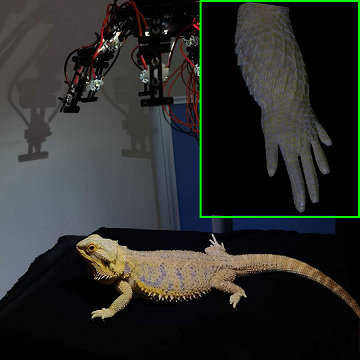
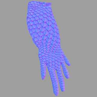
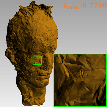
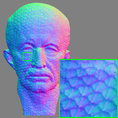
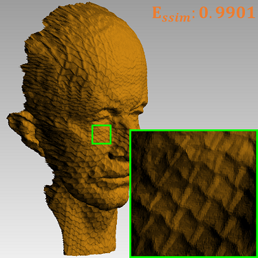
Lizard	Detail component	DGTS [16]	Synthesized normal	Proposed

Figure 9: The geometric texture synthesis result of the Lizard model. The Max Planck model is selected as the target surface with a total of $1,665,036$ vertices. The detail component feature map is captured and extracted as shown in the second figure (Best viewed by zooming in).

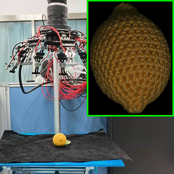
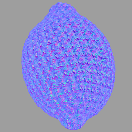
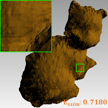
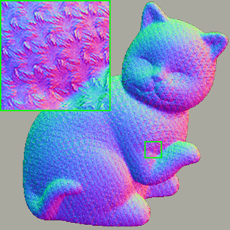
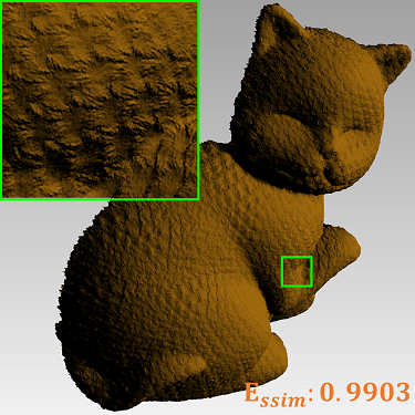
Textile	Detail component	DGTS [16]	Synthesized normal	Proposed

Figure 10: The geometric texture synthesis result of the Textile model. The Cat model is selected as the target surface with a total of $1,999,807$ vertices. The $\mathbf{E}_{ssim}$ value of our proposed method is $0.9903$, while the $\mathbf{E}_{ssim}$ value of DGTS [16] is $0.7180$.

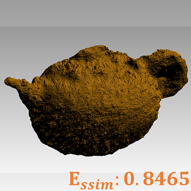
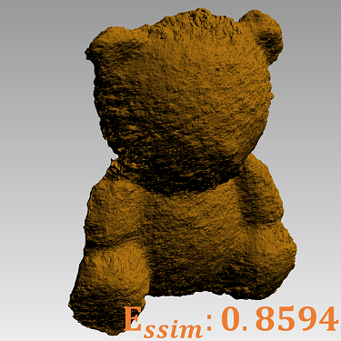
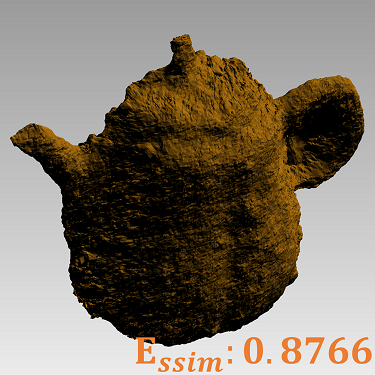
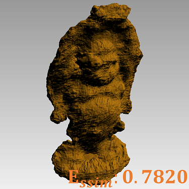
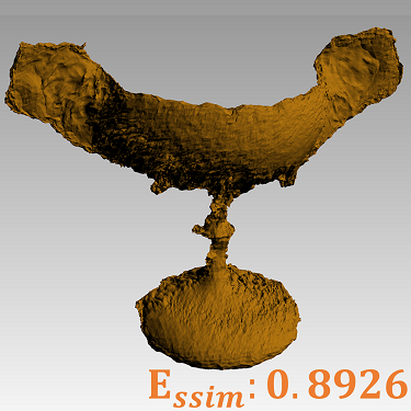
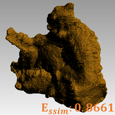
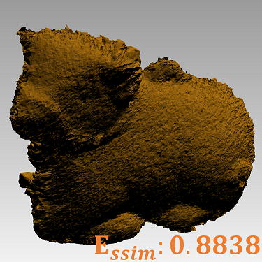
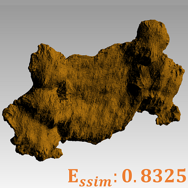
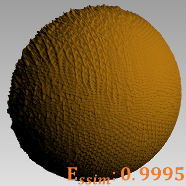
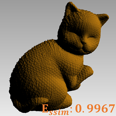
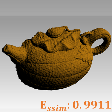
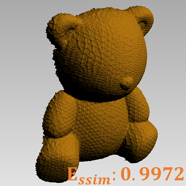
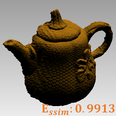
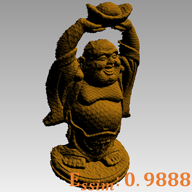
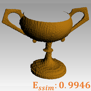
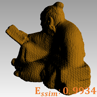
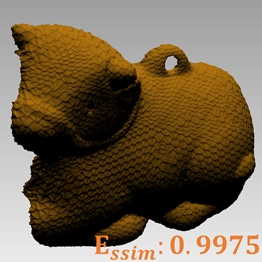
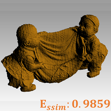
Ball	Cat	Pot1	Bear	Pot2	Buddha	Goblet	Reading	Cow	Harvest

Figure 11: Comparative illustration of geometric texture synthesis on the DiLiGenT dataset [41] using the Lizard skin. The top row are the texture synthesis results of DGTS [16], while the bottom row are the synthesis results of the proposed method. From left to right: The $\mathbf{E}_{ssim}$ results of the detail component in DGTS are provided at the bottom of each reconstructed object. Please zoom-in for details.

5.1 Experimental Protocols

Input data. The proposed framework does not limit the input type of data, as long as it can be converted into a single normal map. It is noted that in this section, all 3D surfaces are reconstructed by the surface from normal (SfN) method [19].

For the input 3D data sources, they mainly come from dense scanning devices. The reason to select these data is due to the fact that they are more challenging and have not yet been properly processed in existing methods. There are two ways to obtain the real and dense data, i.e., by laser scanning or photometric stereo (PS). To this end, we built a PS device consisting of an industrial camera and $36$ LED lights (see Fig. 9) to obtain the real surface normal.

Error measurement. Considering that both the input and output of the proposed method are normals, it is reasonable to compare these results in the normal domain. Thus, the orientation difference between two compared normal vectors is measured by $\mathbf{E}_{mae}$ [19, 43].

$$\small\mathbf{E}_{mae}\left({{\mathcal{N}_{o}},{\mathcal{N}_{t}}}\right)=\frac{1}{|\Omega|}\sum\limits_{\left({r,c}\right)\in\Omega}{\arccos\left({{\mathcal{N}_{o}}\left({r,c}\right)\odot{\mathcal{N}_{t}}\left({r,c}\right)}\right)},$$ (20)

where $|\Omega|$ denotes the total number of all compared normal pairs in $\Omega$, ${\mathcal{N}_{o}}$ represents the reference input, and ${\mathcal{N}_{t}}$ represents the target output. The $\mathbf{E}_{mae}$ value ranges from 0^∘ to 180^∘.

To comprehensively evaluate the generated surface quality, a widely-used structural similarity (SSIM) metric $\mathbf{E}_{ssim}$ in geometric surface processing [45, 46] is used to measure the difference between the original and resulted depths. $\mathbf{E}_{ssim}$ is calculated as the mean of the channel-wise SSIM value, ${\mathbf{E}_{ssim}}\left({{\mathcal{N}_{o}},{\mathcal{N}_{t}}}\right)=\frac{1}{3}\sum\nolimits_{k}{E_{ssim}^{k}\left({\mathcal{N}_{o}^{k},\mathcal{N}_{t}^{k}}\right)}$, where the k-th channel $\small{\mathbf{E}_{ssim}^{k}\left({\mathcal{N}_{o}^{k},\mathcal{N}_{t}^{k}}\right)}$ is defined as

$$\leavevmode\resizebox{408.68454pt}{}{$\mathbf{E}_{ssim}^{k}\left({\mathcal{N}_{o}^{k},\mathcal{N}_{t}^{k}}\right)=\frac{{\left({2\mu_{o}^{k}\mu_{t}^{k}+c1}\right)\left({\sigma_{ot}^{k}+c2}\right)}}{{\left({{{\left({\mu_{o}^{k}}\right)}^{2}}+{{\left({\mu_{t}^{k}}\right)}^{2}}+c1}\right)\left({{{\left({\sigma_{o}^{k}}\right)}^{2}}+{{\left({\sigma_{t}^{k}}\right)}^{2}}+c2}\right)}}$},$$ (21)

where $\mu_{o}^{k}$ is the average of ${\mathcal{N}_{o}^{k}}$, $\mu_{t}^{k}$ is the average of ${\mathcal{N}_{t}^{k}}$, ${{{\left({\sigma_{o}^{k}}\right)}^{2}}}$ is the variance of ${\mathcal{N}_{o}^{k}}$, ${{{\left({\sigma_{t}^{k}}\right)}^{2}}}$ is the variance of ${\mathcal{N}_{t}^{k}}$, and ${\sigma_{ot}^{k}}$ is the covariance of ${\mathcal{N}_{o}^{k}}$ and ${\mathcal{N}_{t}^{k}}$. $c1$ and $c2$ are two constants used to maintain stability, where $c1$ = 0.01 and $c2$ = 0.03, respectively. The $\mathbf{E}_{ssim}$ value ranges from 0 to 1. When two compared images are identical, the $\mathbf{E}_{ssim}$ value is equal to one.

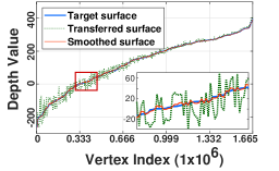
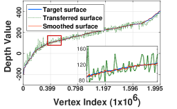
Lizard	Textile

Figure 12: Performance evaluation of the proposed geometric texture synthesis method in terms of the height profile. The blue solid line represents the original depth value, the green dot line represents the transferred depth value, and the red solid line represents the smoothed result of the transferred surface by a 5$\times$5 average filter.

Computing platform. All algorithms in the normal domain are implemented in MATLAB 2018, and performed on a computer with Intel i7-CPU@2.90GHz and $32$GB RAM. In addition, the CNN model is trained and tested on NVIDIA Tesla P100 GPU.

In the experiments, many of the deep learning methods we have compared either do not provide training code or do not provide training databases. On the other hand, the related experiments are used to demonstrate that deep-learned models can be seamlessly embedded into the proposed framework. For a fair comparison, all the compared deep methods except RDN-Net [47] directly adopt the off-the-shelf models provided by the authors.

In the experiments of 3D surface super-resolution, the training of RDN-Net [47] is only trained on the original normal map, and that of “Proposed” denotes that [47] is only trained on the detail component map. The training samples are cropped into 192$\times$192 normal blocks, where the Adam is used as our optimization solver in Python Toolbox PyTorch. The initial learning rate is set to $10e$-$5$ and the batch size is 16. There are a total of $353$ samples used in training, testing, and validating the CNN models. The testing samples are strictly blind to the training process. All other training settings are the same as suggested [47].

TABLE IV: The MAE, SSIM, memory, and time of the transferred result between Circular and Bunny with different resolutions (input points/vertices).

Input points $\#5010$ $\#10106$ $\#20441$ $\#49532$ $\#153145$ $\#306491$ Shape $\mathbf{E}_{mae}$(^∘) DSPL [48] 17.04 16.62 16.37 16.00 n/a n/a LAPL [26] 12.13 11.07 9.05 n/a n/a n/a Proposed 4.97 4.16 3.48 2.79 2.42 2.28 Detail $\mathbf{E}_{mae}$(^∘) DSPL [48] 16.02 23.06 32.15 33.79 n/a n/a LAPL [26] 14.65 17.11 21.78 n/a n/a n/a Proposed 10.71 10.93 10.87 10.90 10.86 10.86 Detail $\mathbf{E}_{ssim}$ DSPL [48] 0.92 0.83 0.74 0.72 n/a n/a LAPL [26] 0.93 0.90 0.86 n/a n/a n/a Proposed 0.9797 0.9809 0.9806 0.9805 0.9808 0.9808 Memory (Mb) DSPL [48] 32.91 67.70 113.22 745.59 n/a n/a LAPL [26] 827.52 3044.78 12620.90 n/a n/a n/a Proposed 5.08 7.11 10.62 19.77 53.50 103.89 Time cost (Sec.) DSPL [48] 11.03 41.62 266.87 2365.20 n/a n/a LAPL [26] 20.93 89.64 383.56 n/a n/a n/a Proposed 0.06 0.19 0.40 0.57 2.93 3.82

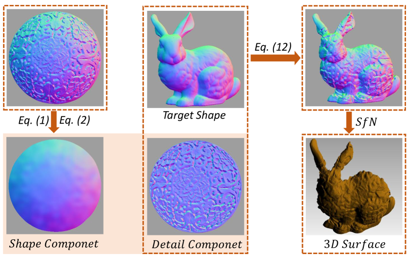
Figure 13: Flowchart of the geometry detail transfer. The shape component and detail component of the source normal are extracted by Eq. (1) and Eq. (2), respectively. Then, the detail component is transferred to the target normal by Eq. (12) and reconstructed by the surface-from-normal (SfN) method [19].

5.2 Geometric Texture Synthesis

In a practical texture synthesis, one common case is that the available source texture is not enough to be allocated on the target shape. One solution is to synthesize more similar textures from the source surface, in order to cover the entire target surface shape. Unfortunately, existing geometry texture synthesis methods have not been well developed to deal with a dense and irregular texture pattern. In this section, the experiments are carried out by showing that the proposed detail component can be used as a standalone feature map due to its detail separability property, and hence it is possible to solve the problem of geometric texture synthesis.

Specifically, for a small piece of the source surface, its detail component is separated first, and then used to be synthesized in the feature map domain. In general, all the image texture synthesis methods are applicable to our proposed. For simplicity, we select a representative method [44] to demonstrate the synthesis performance of the detail component. The synthesized result is then used to transfer on an entire target surface shape. The overall pipeline of the proposed geometric texture synthesis scheme is illustrated in Fig. 8.

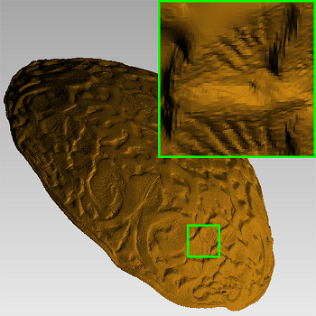
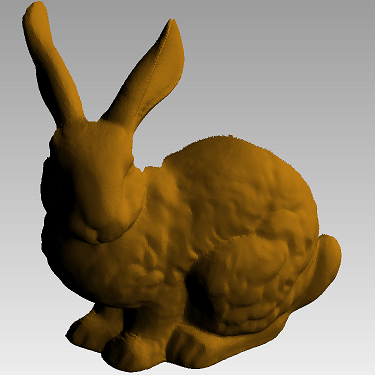
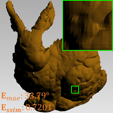
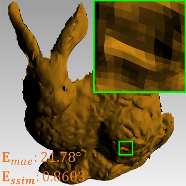
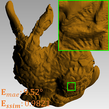
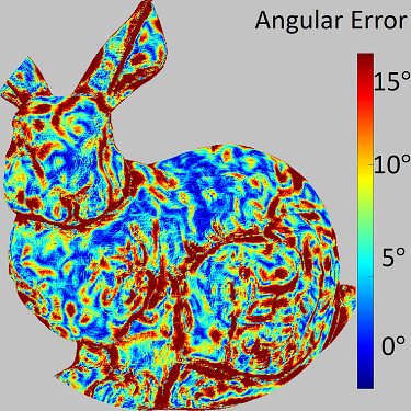
Original surface	Target surface	DSPL [48]	LAPL [26]	Proposed	Energy map

Figure 14: Illustration of the geometry detail transfer for the Bunny model. The original surface is Circular with the total vertex number of $646,693$. The detail component feature map used for transfer is reconstructed and shown in the right-top green box. The energy map of angular error is measured between the original detail component and our transferred one, and $\mathbf{E}_{mae}$ is $9.52^{\circ}$.

Fig. 9 shows a lizard, which is reconstructed by our photometric stereo setup. It is noted that only a part of the scanned skin normal data is used for synthesis, and is named as the Lizard model. One latest deep-learned geometry synthesis method DGTS [16] is used for comparison. As seen in Fig. 9, DGTS cannot properly synthesize the dense and non-repetitive texture pattern, where the $\mathbf{E}_{ssim}$ value is only $0.7740$. The main reason is that its ability to capture the texture feature depends on the receptive field. In addition, it also has the disadvantage of incurring heavy time cost and excessive memory cost, e.g., $233$Sec and $14,216$Mb. In contrast, the transferred result of our method has the $\mathbf{E}_{ssim}$ value of $0.9901$, and the running time and memory costs are $11.88$Sec and $857$Mb, respectively.

Fig. 10 shows another synthesis example with complex textures, where the reconstructed Textile model is used as the source detail component, and the Cat model is used as the target shape. While DGTS [16] produces a poor geometric texture synthesis result, where the related $\mathbf{E}_{ssim}$ value of the detailed component between the original and DGTS is 0.7180, and our method generates a satisfying texture synthesis result, where the related $\mathbf{E}_{ssim}$ value is 0.9903.

Fig. 11 provides the overall visual results of geometric texture synthesis on the DiLiGenT dataset [41]. As seen, our proposed texture synthesis scheme can preserve the geometric details of the original surface as well as the surface shape of the target 3D model. DGTS [16] produces obviously worse synthesized results than the proposed method. At the same time, DGTS also deteriorates the target shape. For example, the face of Buddha by DGTS is difficult to be perceived.

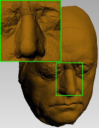
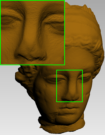
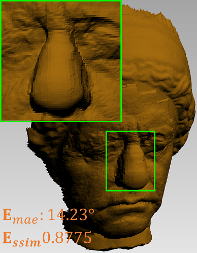
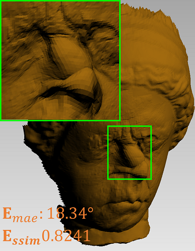
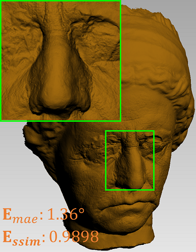
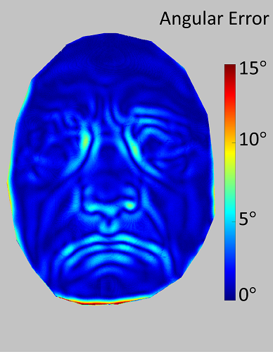
Original surface	Target surface	DSPL [48]	LAPL [26]	Proposed	Energy map

Figure 15: Performance comparisons of the local transfer. The local face of Venus is replaced by Goethe, where the source Goethe has the total vertex number of $539,352$. A partial zoom-in part is shown in the left-top green box. The energy map of angular error is measured between the original detail component and our transferred one, and $\mathbf{E}_{mae}$ is $1.36^{\circ}$.

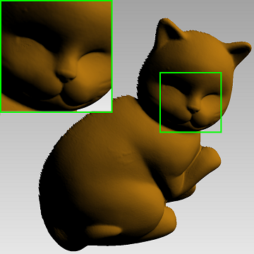
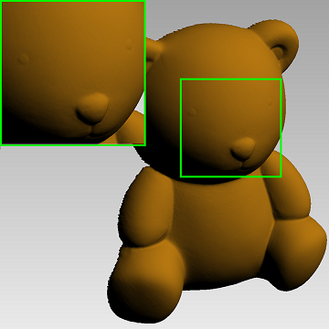
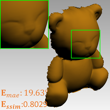
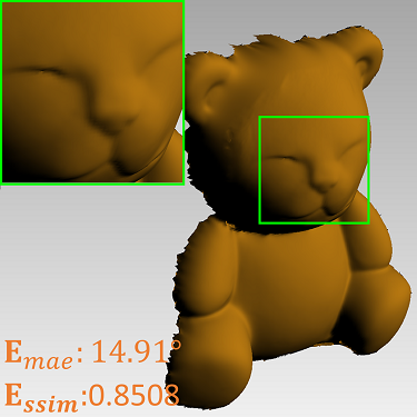
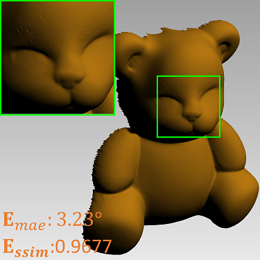
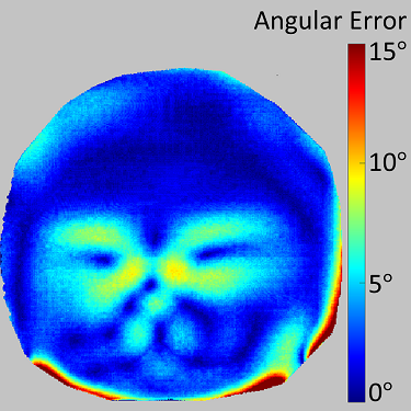
Original surface	Target surface	DSPL [48]	LAPL [26]	Proposed	Energy map

Figure 16: Performance comparisons of the local transfer. The local face of Bear is replaced by Cat, where the source Cat has the total vertex number of $119,389$. A zoom-in part is shown in the left-top green box. The energy map of angular error is measured between the original detail component and our transferred one, and $\mathbf{E}_{mae}$ is $3.23^{\circ}$.

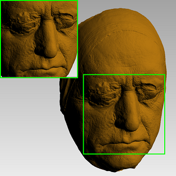
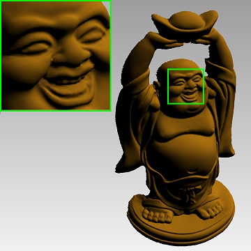
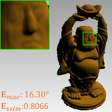
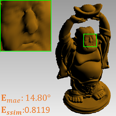
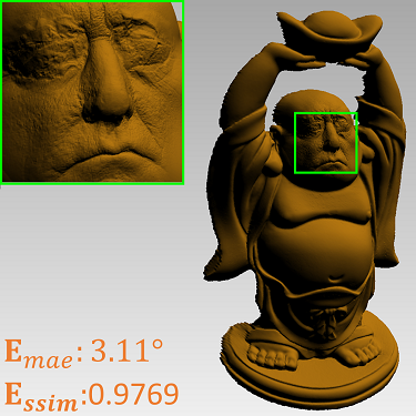
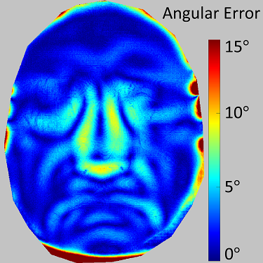
Original surface	Target surface	DSPL [48]	LAPL [26]	Proposed	Energy map

Figure 17: Performance comparisons of the local transfer. The local face of Buddha is replaced by Goethe, where the source Goethe has the total vertex number of $334,696$. A zoom-in part is shown in the left-top green box. The energy map of angular error is measured between the original detail component and our transferred one, and $\mathbf{E}_{mae}$ is $3.11^{\circ}$.

Moreover, we evaluate the transferred surface using the height profile as shown in Fig. 12, where the depth values of a target surface are firstly reordered in an ascending order, and the related depth values of a transferred surface are plotted according to their positions. The depth values of the proposed method are similar to the target surface, which also validates the shape similarity in the property of the detail transferability.

5.3 Geometry Detail Transfer

For geometry detail transfer, the detail component and shape component of the source and target surfaces are separated by Eq. (1) and Eq. (2), respectively. The proposed detail transfer scheme is illustrated in Fig. 13. The detail component of the original surface is transferred to the shape component of the target surface. In this section, the performance of the geometry detail transfer is evaluated and compared with two mesh-based surface editing methods.

The whole source surface is transferred to a target shape, which is marked as global transfer. Fig. 14 shows that Bunny is transferred with the geometry details of Circular. The Circular model is a high-definition laser-scanning data downloaded from Aim@Shape, and its normal map with resolution of $1000\times 1000$ are obtained by MeshLab as the input. Two mesh-based methods, i.e., the Laplace mesh editing method (denoted as LAPL) [26] and the normal displacement method (denoted as DSPL) [48], are used for comparisons. Compared with the proposed method, neither of them can properly deal with the real dense surface. In addition, the transferred surface is evaluated in both the shape and detail aspects. For surface shape comparison, the $\mathbf{E}_{mae}$ error between the shape component of Bunny and that of the transferred result is calculated. For geometry details comparison, the $\mathbf{E}_{mae}$ and $\mathbf{E}_{ssim}$ results between the detail component of Circular and that of the transferred result are also obtained. Table IV provides the detailed MAE, SSIM, memory, and running time of the transfer process between Circular and Bunny with various resolutions (input points/vertices), where “n/a” denotes that the results can not be obtained on the current computing platform. For instance, under the same amount of the input vertices, like $5,000$, LAPL requires more than $800$Mb memory, which is $162$ times of ours. What makes the matter worse is that the memory gap increases exponentially with the number of input vertices. As for the time cost comparison, our method can calculate the dense surface in a trivial amount of time compared with DSPL and LAPL.

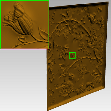
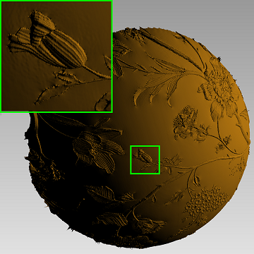
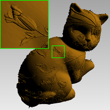
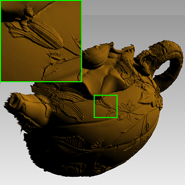
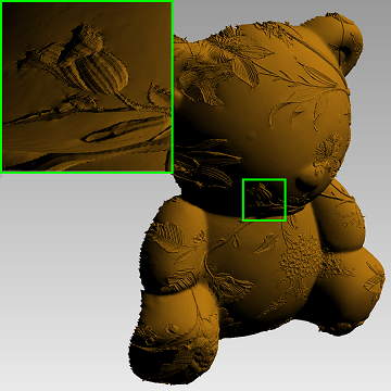
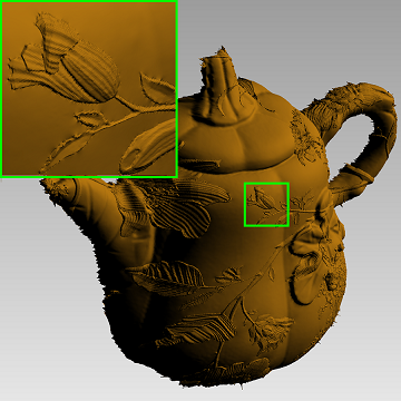
Original surface	Ball	Cat	Pot1	Bear	Pot2
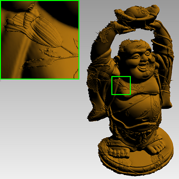
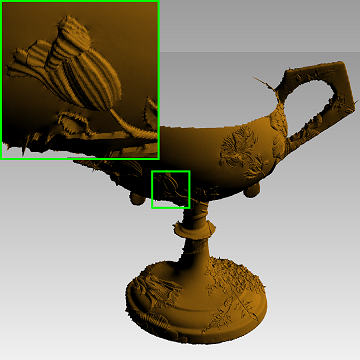
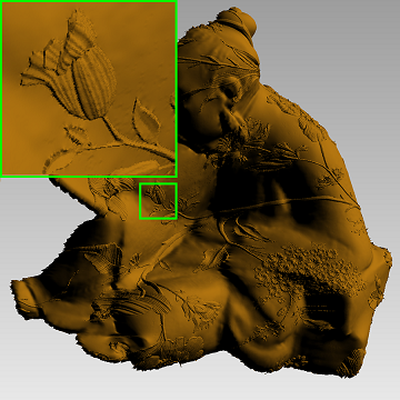
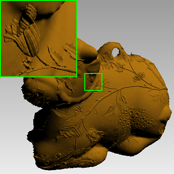
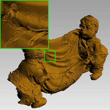
Normal	Buddha	Goblet	Reading	Cow	Harvest

Figure 18: Performance comparisons of the global transfer. The original model Flower is transferred on the DiLiGenT dataset [41]. A zoom-in part is shown in the left-top green box.

TABLE V: Quantitative results of the geometric detail transfer on the latest DiLiGenT dataset [41].

Method Ball Cat Pot1 Bear Pot2 Buddha Goblet Reading Cow Harvest Shape $\mathbf{E}_{mae}$(^∘) DSPL [48] 4.10 5.93 8.83 7.13 3.18 4.90 4.82 9.43 4.04 2.51 LAPL [26] 1.73 2.22 2.85 3.17 4.37 6.49 3.39 3.02 2.25 6.10 Proposed 1.83 2.02 2.49 1.96 2.26 2.54 2.90 2.09 1.90 2.43 Shape $\mathbf{E}_{ssim}$ DSPL [48] 0.9895 0.9944 0.9868 0.9827 0.9979 0.9950 0.9972 0.9744 0.9945 0.9992 LAPL [26] 0.9983 0.9990 0.9984 0.9956 0.9959 0.9916 0.9987 0.9979 0.9988 0.9946 Proposed 0.9990 0.9995 0.9995 0.9994 0.9995 0.9994 0.9994 0.9994 0.9995 0.9994 Detail $\mathbf{E}_{mae}$(^∘) DSPL [48] 16.15 19.67 24.31 19.91 19.57 26.17 24.63 23.73 16.90 20.50 LAPL [26] 13.90 17.53 18.73 15.19 18.14 24.71 20.03 18.03 15.13 21.73 Proposed 1.43 4.13 6.83 3.55 6.17 13.02 5.69 5.67 3.57 10.63 Detail $\mathbf{E}_{ssim}$ DSPL [48] 0.9088 0.9205 0.9307 0.8959 0.9443 0.9158 0.9531 0.8826 0.9265 0.9291 LAPL [26] 0.9385 0.9445 0.9603 0.9438 0.9491 0.9269 0.9665 0.9369 0.9513 0.9251 Proposed 0.9994 0.9964 0.9933 0.9966 0.9933 0.9805 0.9966 0.9933 0.9971 0.9848 Memory (Mb) DSPL [48] 305.24 305.23 310.66 301.87 304.72 308.43 303.31 311.93 304.59 311.30 LAPL [26] 12183.22 11616.61 11694.25 11587.38 12276.66 11988.65 12760.16 11457.79 11853.22 10910.99 Proposed 17.66 18.75 21.76 17.64 19.91 19.23 25.82 17.63 17.39 20.10 Time cost (sec.) DSPL [48] 5.26 5.05 4.88 4.60 4.64 4.87 4.61 4.83 4.77 4.44 LAPL [26] 696.67 658.30 688.34 586.96 675.27 819.87 676.72 706.23 647.91 733.78 Proposed 0.50 0.48 0.52 0.40 0.44 0.50 0.59 0.42 0.47 0.50

Different from the global transfer, local transfer means that a local geometry feature is transferred to the target surface, which can be regarded as coarse-grained detail transfer. It is worth noting that the detail granularity depends on that, the closer the shape component in Eq. (1) is to the original surface, the finer the granularity of the detail component in Eq. (2), and vice versa. Fig. 15 shows an interesting example of the local transfer, where the face of Venus (downloaded from Aim@Shape) zoomed in the green bounding box is replaced by Goethe. Goethe is used to extract the coarse-grained detail by setting a large filter size ($w$=10) in Eq. (1) to get the coarse geometry feature. The transferred results show that LAPL [26] and DSPL [48] cannot preserve the nose shape of Goethe. Meanwhile, the proposed method generates the best visual effect, where the transferred nose shape is almost the same as the original one. The transferred face region of our method has the $\mathbf{E}_{mae}$ value of $1.36^{\circ}$ and the $\mathbf{E}_{ssim}$ value of $0.9898$, respectively. Figs. 16 and 17 show another two examples of the local surface transfer. The transferred faces of Cat and Goethe are satisfactorily matched with the target shapes, which further demonstrate the effectiveness of the proposed normal-based detail representation.

In addition, Table V provides the quantitative evaluation results for the geometric detail transfer on the DiLiGenT dataset [41], and the relevant visual results are provided in Fig. 18. We provide the detailed results by transferring Flowers to ten different target surfaces. The average results of the shape MAE for DSPL, LAPL and our method are 5.48^∘, 3.56^∘, and 2.24^∘, respectively. Meanwhile, the average results of the detail MAE for DSPL, LAPL, and our method are 21.15^∘, 18.31^∘, and 6.07^∘, respectively. It shows that our method can greatly improve the shape and detail transfer performance compared with DSPL and LAPL. In addition, we run the same experiments for ten times to collect the average of memory cost (Mb) and time cost (Sec) to measure the efficiency of each scheme. While the average results of the memory consumption for DSPL, LAPL and our method are 306.73, 11833.11, and 19.59, respectively, the average results of the time complexity for DSPL, LAPL and our method are 4.79, 689.01, and 0.48, respectively. As seen, our method is highly efficient compared with DSPL and LAPL in terms of both the memory and time costs.

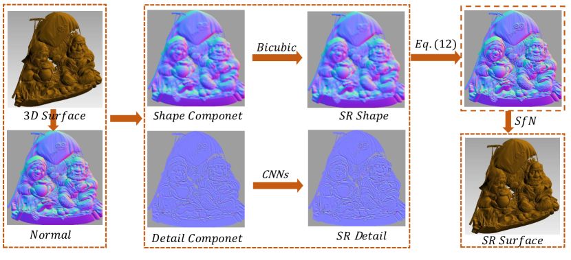
Figure 19: Pipeline of the proposed 3D surface super-resolution. The shape component and detail component of the original normal are obtained by Eq. (1) and Eq. (2), respectively. Then, the shape component and the detail component are up-sampled to the desired size through the bicubic interpolation and RDN-Net [47], respectively. Finally, the super-resolution result is obtained by Eq. (12) and reconstructed by the SfN method [19].

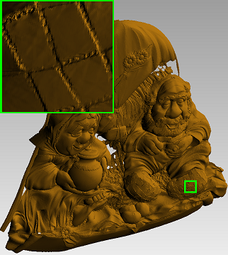
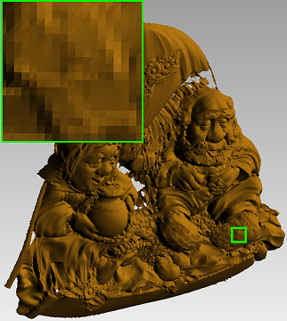
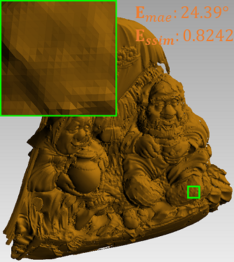
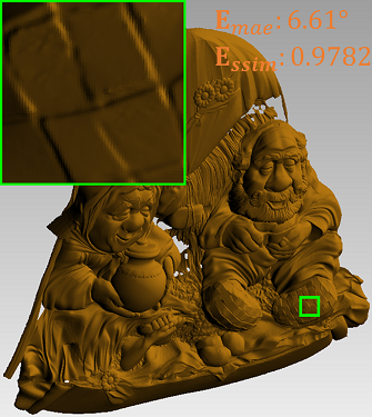
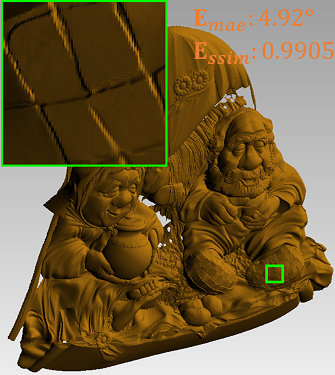
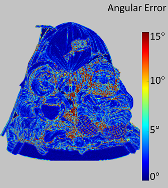
Reference surface	Low-resolution surface	PU-Net [49]	RDN-Net [47]	Proposed	Energy map

Figure 20: Comparison results of 3D surface super-resolution for the Panno model. The $\mathbf{E}_{mae}$ and $\mathbf{E}_{ssim}$ results of the proposed method are $4.92^{\circ}$ and $0.9905$, those of PU-Net [49] are $24.39^{\circ}$ and $0.8242$, and those of RDN-Net [47] are $6.61^{\circ}$ and $0.9782$, respectively. The angular error map of our method is shown on the most right-hand side.

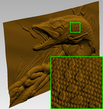
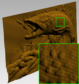
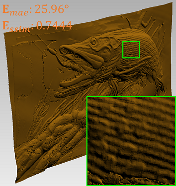
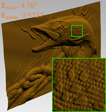
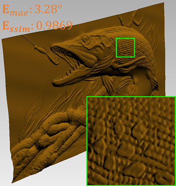
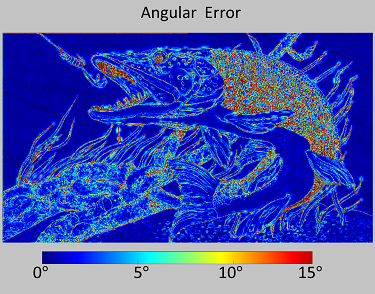
Reference surface	Low-resolution surface	PU-Net [49]	RDN-Net [47]	Proposed	Energy map

Figure 21: Comparison results of 3D surface super-resolution for the Fish model. The $\mathbf{E}_{mae}$ and $\mathbf{E}_{ssim}$ values of the proposed method are $3.28^{\circ}$ and $0.9869$, those of PU-Net [49] are $25.96^{\circ}$ and $0.7444$, and those of RDN-Net [47] are $4.78^{\circ}$ and $0.9757$, respectively. The angular error map of our method is shown on the most right-hand side.

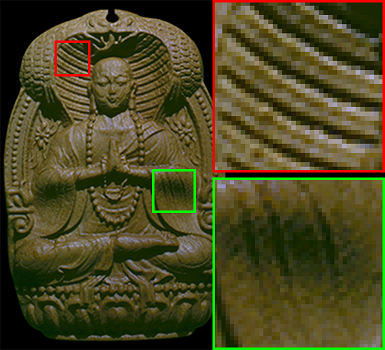
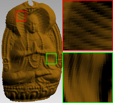
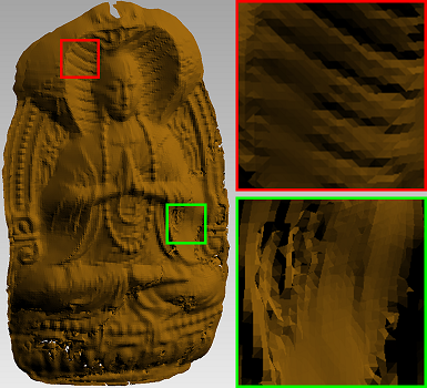
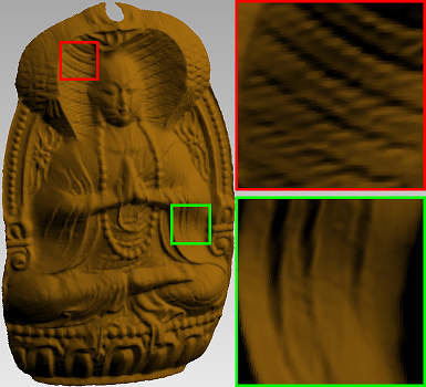
Captured image	Low-resolution surface	PU-Net[49]	RDN-Net [47]	Proposed

Figure 22: Comparison results of 3D surface super-resolution for the Woodcarving model. The associated normal map is obtained by our photometric stereo device. Content in the red and green boxes is zoomed-in and shown on the right hand side for each image.

5.4 3D Surface Super-resolution

The proposed detail component can also be applied to 3D surface super-resolution based on existing learned CNN models. Specifically, for a low-resolution surface, we first decouple its normal map into the shape component and the detail component. Since the former is really smooth, it can be up-sampled by a simple method such as Bicubic. Since the latter is really complex, it can be enhanced by an advanced image-based super-resolution network. The enhanced detail component and shape component are then converted back, and finally the super-resolution 3D surface can be generated. The pipeline of our surface super-resolution scheme is illustrated in Fig. 19.

In principle, the proposed detail component can be compatible with all existing image super-resolution networks if they are properly trained in the normal domain. To verify the performance, we have carried out three different comparison experiments to verify the super-resolution performance. Fig. 20 shows the original Panno model with the size of 1812$\times$1800 downsampled by $\frac{1}{4}\times\frac{1}{4}$ first, and then used as the input for 4$\times$4 enhancement. PU-Net [49] provides a smooth result, the upsampled Panno has the $\mathbf{E}_{mae}$ value of $24.39^{\circ}$ and the $\mathbf{E}_{ssim}$ value of $0.8242$. Compared with PU-Net, RDN-Net [47] greatly restore the relevant surface details. Meanwhile, our method can effectively enhance the upsampled surface with the $\mathbf{E}_{mae}$ value of $4.92^{\circ}$ and the $\mathbf{E}_{ssim}$ value of $0.9905$, respectively.

Fig. 21 provides another 4$\times$4 Fish super-resolution with the original size of 339$\times$192. As seen, the low-resolution surface has blurring fish scale. While PU-Net [49] can reduce the blurring effect, it can cause line-like artifact with the $\mathbf{E}_{mae}$ value of $25.96^{\circ}$ and the $\mathbf{E}_{ssim}$ value of $0.7444$. RDN-Net [47] generates a better result than PU-Net, but the edge of fish scale is not obvious. In contrast, our proposed method achieves the best visual effect with the sharp edge of fish scale, where the $\mathbf{E}_{mae}$ value is $3.28^{\circ}$ and the $\mathbf{E}_{ssim}$ value is $0.9869$, respectively.

Fig. 22 illustrates a real-world low-resolution Woodcarving model with the normal size of 126$\times$187 obtained by our photometric stereo setup used for 4$\times$4 enhancement. In general, three methods can restore some surface details. However, when we zoom-in the relevant super-resolution results, our method generates the best restoration performance compared with PU-Net [49] and RDN-Net [47].

6 Discussions

In the proposed framework, a 3D surface is not expressed by meshes, voxels, point clouds, or octrees [50]. Instead, the orientation of a surface patch, known as the normal vector, is comprehensively explored as a new representation for 3D surface geometry details. To obtain the normal map of a surface, the surface points need to be projected onto the viewing plane to obtain the corresponding normal vector “pixel”. Our main focus is to investigate and validate the relationship between the shape and geometry details based on the single-view normal domain, and the quality can be affected if there are self-occlusions or discontinuities in an input normal image.

As seen in Fig. 3, the error maps between the shape of ${{\bar{\Delta}}_{\mathcal{N}}}$ and $\mathbf{z}$ are dark-blue overall (with the average MAE value $0.86^{\circ}$), and large errors are shown in light-blue distributed over self-occluded surface regions, such as the nose boundary of Geothe and the paw boundaries of Lizard. The main reason is that normals on the self-occlusion regions are not properly captured in a single-view normal map, affecting the accuracy of the extracted detail component. The similar phenomenon can be observed in geometry detail transfer (see Fig. 14, Fig. 15, Fig. 16, and Fig. 17) and 3D surface super-resolution (see Fig. 20 and Fig. 21). It is worth noting that in addition to self-occlusion from the source surface, self-occlusion from the target surface also leads to major errors in geometry detail transfer. A representative case can be found in Fig. 14, where the target surface of Bunny contains a lot of self-occlusions (with the average MAE value $9.52^{\circ}$) on its neck, ears, tail, and gaps between legs. Fortunately, most of these local distortions are acceptable in our extensive experiments. For an interested surface with serious self-occlusion, multiple-view normal maps are required, which is discussed in the future work.

In addition, the form of a normal map brings an extraordinary convenience to process 3D surface, which also means that it is not a “what you see is what you get” paradigm. To obtain a 3D surface result, we have to resort to the SfN tool. It is worth noting that the surface discontinuity is one of the main problems in the single-view reconstruction [51], which often happens under the condition of self-occlusion due to the loss of depth information. This is also an open problem for all SfN methods. As a result, the final surface will also be affected by SfN in our proposed framework.

In summary, the detail theory we developed offers new insights into the 3D surface processing, enabling the two basic elements of 3D surface, shape and geometric details, to be separately expressed and effectively processed. This will bring the versatility of various image processing methods into 3D surface processing, which have been validated by some applications as described in Section 5. Finally, while existing mesh-based methods show huge limitations in dense 3D surface processing due to their high computing time and excessive memory costs, our proposed has illustrated significant advantages in addressing these difficulties.

7 Conclusion and Future Work

In this article, a new surface detail representation is developed for 3D surface geometry processing in normal domain, where surface geometry details are separated from a surface normal map as a shape-uncorrelative feature with high transferability. We also show that the dense laser-scanning point clouds can be satisfactorily processed when converting the orientation of each surface patch into a normal vector. To illustrate the versatility of our proposed, we further design three popular surface geometry detail processing algorithms based on the proposed normal-based framework. Experimental results validate the superiority of the proposed surface detail representation, and we believe that it will offer new insights into many 3D surface processing problems.

For future research, some further explorations can be developed in the following aspects to improve the performance of the proposed normal-based detail representation. First, the current design is simple and efficient for a single-view 3D surface, but their feature representation capabilities are limited to self-occlusion. A new normal map will be investigated to record both visible and invisible micro-geometry features in a single image, due to the fact that the current camera imaging projection, which is the main reason to result in occlusion features, is not a necessary way to record a surface normal. Second, the proposed method is effective on a single-view 3D surface. However, its performance on a multiple-view case [52] is unknown and hence need to be investigated, where the self-occlusion or discontinuity may no longer be a problem. Third, due to the fact that the quality of service for dynamic moving objects is becoming more and more popular, it is worthwhile to further extend this study to solving the geometric detail processing of dynamic point clouds (DPC).

8 Acknowledgments

The authors would like to give thanks to Mr. Maolin Cui for the preparations of the experimental data and the Python implementation, and would also like to express their sincere gratitude to the anonymous reviewers for valuable comments and suggestions.

References

- [1] Robert L Cook. Shade trees. In Annual Conference on Computer Graphics and Interactive Techniques (SIGGRAPH), pages 223–231, 1984.
- [2] Tolga Tasdizen, Ross Whitaker, Paul Burchard, and Stanley Osher. Geometric surface smoothing via anisotropic diffusion of normals. In IEEE Visualization, pages 125–132, 2002.
- [3] Qingyang Tan, Lin Gao, Yu-Kun Lai, and Shihong Xia. Variational autoencoders for deforming 3D mesh models. In IEEE Conference on Computer Vision and Pattern Recognition (CVPR), pages 5841–5850, 2018.
- [4] Xianzhi Li, Ruihui Li, Lei Zhu, Chi-Wing Fu, and Pheng-Ann Heng. DNF-Net: a Deep Normal Filtering Network for Mesh Denoising. IEEE Transactions on Visualization and Computer Graphics, pages 1–13, 2020.
- [5] Suryansh Kumar, Yuchao Dai, and Hongdong Li. Superpixel soup: Monocular dense 3D reconstruction of a complex dynamic scene. IEEE Transactions on Pattern Analysis and Machine Intelligence, 43(5):1705–1717, 2021.
- [6] Lifeng Wang, Xi Wang, Xin Tong, Stephen Lin, Shimin Hu, Baining Guo, and Heung-Yeung Shum. View-dependent displacement mapping. ACM Transactions on Graphics, 22(3):334–339, 2003.
- [7] Xi Wang, Xin Tong, Stephen Lin, Shimin Hu, Baining Guo, and Heung-Yeung Shum. Generalized displacement maps. In Eurographics Workshop on Rendering, pages 227–233, 2004.
- [8] Pravin Bhat, Stephen Ingram, and Greg Turk. Geometric texture synthesis by example. In ACM SIGGRAPH Symposium on Geometry Processing, pages 41–44, 2004.
- [9] Konstantinos Rematas and Vittorio Ferrari. Neural voxel renderer: Learning an accurate and controllable rendering tool. In IEEE Conference on Computer Vision and Pattern Recognition (CVPR), pages 5417–5427, 2020.
- [10] Marc Alexa. Differential coordinates for local mesh morphing and deformation. The Visual Computer, 19(2-3):105–114, 2003.
- [11] Andy Zeng, Shuran Song, Matthias Niessner, Matthew Fisher, Jianxiong Xiao, and Thomas Funkhouser. 3DMatch: Learning Local Geometric Descriptors From RGB-D Reconstructions. In IEEE Conference on Computer Vision and Pattern Recognition (CVPR), pages 1802–1811, 2017.
- [12] Jinghua Wang and Jianmin Jiang. Learning across tasks for zero-shot domain adaptation from a single source domain. IEEE Transactions on Pattern Analysis and Machine Intelligence, pages 1–15, 2021.
- [13] Guanying Chen, Kai Han, Boxin Shi, Yasuyuki Matsushita, and Kwan-Yee Kenneth Wong. Deep photometric stereo for non-lambertian surfaces. IEEE Transactions on Pattern Analysis and Machine Intelligence, pages 1–14, 2020.
- [14] Yakun Ju, Junyu Dong, and Sheng Chen. Recovering surface normal and arbitrary images: A dual regression network for photometric stereo. IEEE Transactions on Image Processing, 30:3676–3690, 2021.
- [15] Sema Berkiten, Maciej Halber, Justin Solomon, Chongyang Ma, Hao Li, and Szymon Rusinkiewicz. Learning detail transfer based on geometric features. Wiley Computer Graphics Forum, 36(2):361–373, 2017.
- [16] Amir Hertz, Rana Hanocka, Raja Giryes, and Daniel Cohen-Or. Deep geometric texture synthesis. ACM Transactions on Graphics, 39(4), 2020.
- [17] Michael Bass, Casimer DeCusatis, Jay Enoch, Vasudevan Lakshminarayanan, Guifang Li, Carolyn Macdonald, Virendra Mahajan, and Eric Van Stryland. Handbook of optics, Volume II: Design, fabrication and testing, sources and detectors, radiometry and photometry. McGraw-Hill, Inc., 2009.
- [18] Tolga Tasdizen, Ross Whitaker, Paul Burchard, and Stanley Osher. Geometric surface processing via normal maps. ACM Transactions on Graphics, 22(4):1012–1033, 2003.
- [19] Wuyuan Xie, Yunbo Zhang, Charlie CL Wang, and Ronald C-K Chung. Surface-from-gradients: An approach based on discrete geometry processing. In IEEE Conference on Computer Vision and Pattern Recognition (CVPR), pages 2195–2202, 2014.
- [20] Satoshi Ikehata, David Wipf, Yasuyuki Matsushita, and Kiyoharu Aizawa. Photometric stereo using sparse bayesian regression for general diffuse surfaces. IEEE Transactions on Pattern Analysis and Machine Intelligence, 36(9):1816–1831, 2014.
- [21] Wuyuan Xie, Chengkai Dai, and Charlie CL Wang. Photometric stereo with near point lighting: A solution by mesh deformation. In IEEE Conference on Computer Vision and Pattern Recognition (CVPR), pages 4585–4593, 2015.
- [22] Donghyeon Cho, Yasuyuki Matsushita, Yu-Wing Tai, and In So Kweon. Semi-calibrated photometric stereo. IEEE Transactions on Pattern Analysis and Machine Intelligence, 42(1):232–245, 2018.
- [23] Leif Kobbelt, Swen Campagna, Jens Vorsatz, and Hans-Peter Seidel. Interactive multi-resolution modeling on arbitrary meshes. In Annual Conference on Computer Graphics and Interactive Techniques (SIGGRAPH), pages 105–114, 1998.
- [24] David S Ebert, F Kenton Musgrave, Darwyn Peachey, Ken Perlin, and Steven Worley. Texturing & modeling: a procedural approach. Morgan Kaufmann, 2003.
- [25] Igor Guskov, Wim Sweldens, and Peter Schröder. Multiresolution signal processing for meshes. In Annual Conference on Computer Graphics and Interactive Techniques (SIGGRAPH), pages 325–334, 1999.
- [26] Olga Sorkine, Daniel Cohen-Or, Yaron Lipman, Marc Alexa, Christian Rössl, and H-P Seidel. Laplacian surface editing. In ACM SIGGRAPH Symposium on Geometry Processing, pages 175–184, 2004.
- [27] Aleksey Golovinskiy, Wojciech Matusik, Hanspeter Pfister, Szymon Rusinkiewicz, and Thomas Funkhouser. A statistical model for synthesis of detailed facial geometry. ACM Transactions on Graphics, 25(3):1025–1034, 2006.
- [28] Henning Biermann, Ioana Martin, Fausto Bernardini, and Denis Zorin. Cut-and-paste editing of multiresolution surfaces. ACM Transactions on Graphics, 21(3):312–321, 2002.
- [29] Adam Finkelstein and David H Salesin. Multiresolution curves. In Annual Conference on Computer Graphics and Interactive Techniques (SIGGRAPH), pages 261–268, 1994.
- [30] Emil Praun, Wim Sweldens, and Peter Schröder. Consistent mesh parameterizations. In Annual Conference on Computer Graphics and Interactive Techniques (SIGGRAPH), pages 179–184, 2001.
- [31] Mario Botsch and Leif Kobbelt. Multiresolution surface representation based on displacement volumes. 22(3):483–491, 2003.
- [32] Y-K Lai, S-M Hu, DX Gu, and Ralph R Martin. Geometric texture synthesis and transfer via geometry images. In ACM Symposium on Solid and physical modeling, pages 15–26, 2005.
- [33] Mingqiang Wei, Yidan Feng, and Honghua Chen. Selective guidance normal filter for geometric texture removal. IEEE Transactions on Visualization and Computer Graphics, 27(12):4469–4482, 2021.
- [34] Mengyu Jennifer Kuo, Satoshi Murai, Ryo Kawahara, Shohei Nobuhara, and Ko Nishino. Surface normals and shape from water. IEEE Transactions on Pattern Analysis and Machine Intelligence, pages 1–12, 2021.
- [35] Albert Chern, Felix Knöppel, Ulrich Pinkall, and Peter Schröder. Shape from metric. ACM Transactions on Graphics, 37(4):1–17, 2018.
- [36] Ruihui Li, Xianzhi Li, Ka-Hei Hui, and Chi-Wing Fu. Sp-gan: Sphere-guided 3d shape generation and manipulation. ACM Transactions on Graphics, 40(4):1–12, 2021.
- [37] Chun-Yen Chen and Kuo-Young Cheng. A sharpness dependent filter for mesh smoothing. Elsevier Computer Aided Geometric Design, 22(5):376–391, 2005.
- [38] Tomoaki Higo, Yasuyuki Matsushita, Neel Joshi, and Katsushi Ikeuchi. A hand-held photometric stereo camera for 3-D modeling. In IEEE International Conference on Computer Vision (ICCV), pages 1234–1241, 2009.
- [39] Guillermo Gallego and Anthony Yezzi. A compact formula for the derivative of a 3-D rotation in exponential coordinates. Springer Journal of Mathematical Imaging and Vision, 51(3):378–384, 2015.
- [40] Zhou Wang, Alan C Bovik, Hamid R Sheikh, and Eero P Simoncelli. Image quality assessment: from error visibility to structural similarity. IEEE Transactions on Image Processing, 13(4):600–612, 2004.
- [41] Boxin Shi, Zhipeng Mo, Zhe Wu, Dinglong Duan, Sai-Kit Yeung, and Ping Tan. A benchmark dataset and evaluation for non-lambertian and uncalibrated photometric stereo. IEEE Transactions on Pattern Analysis and Machine Intelligence, 41(2):271–284, 2019.
- [42] Thomas Malzbender, Bennett Wilburn, Dan Gelb, and Bill Ambrisco. Surface enhancement using real-time photometric stereo and reflectance transformation. Rendering Techniques, 2006:245–250, 2006.
- [43] Hiroaki Santo, Masaki Samejima, Yusuke Sugano, Boxin Shi, and Yasuyuki Matsushita. Deep photometric stereo network. In IEEE International Conference on Computer Vision (ICCV) Workshops, pages 501–509, 2017.
- [44] Alexei A Efros and Thomas K Leung. Texture synthesis by non-parametric sampling. In IEEE International Conference on Computer Vision (ICCV), pages 1033–1038, 1999.
- [45] Thiemo Alldieck, Gerard Pons-Moll, Christian Theobalt, and Marcus Magnor. Tex2shape: Detailed full human body geometry from a single image. In IEEE International Conference on Computer Vision (ICCV), pages 2293–2303, 2019.
- [46] Xiaowei Yuan and In Kyu Park. Face de-occlusion using 3D morphable model and generative adversarial network. In IEEE International Conference on Computer Vision (ICCV), pages 10062–10071, 2019.
- [47] Yulun Zhang, Yapeng Tian, Yu Kong, Bineng Zhong, and Yun Fu. Residual dense network for image super-resolution. In IEEE Conference on Computer Vision and Pattern Recognition (CVPR), pages 2472–2481, 2018.
- [48] Mario Botsch, Leif Kobbelt, Mark Pauly, Pierre Alliez, and Bruno Lévy. Polygon mesh processing. CRC press, 2010.
- [49] Lequan Yu, Xianzhi Li, Chi-Wing Fu, Daniel Cohen-Or, and Pheng-Ann Heng. PU-net: Point cloud upsampling network. In IEEE Conference on Computer Vision and Pattern Recognition (CVPR), pages 2790–2799, 2018.
- [50] Peng-Shuai Wang, Yang Liu, Yu-Xiao Guo, Chun-Yu Sun, and Xin Tong. O-cnn: Octree-based convolutional neural networks for 3d shape analysis. ACM Transactions On Graphics, 36(4):1–11, 2017.
- [51] Wuyuan Xie, Miaohui Wang, Mingqiang Wei, Jianmin Jiang, and Jing Qin. Surface reconstruction from normals: A robust dgp-based discontinuity preservation approach. In IEEE Conference on Computer Vision and Pattern Recognition (CVPR), pages 5328–5336, 2019.
- [52] Min Li, Zhenglong Zhou, Zhe Wu, Boxin Shi, Changyu Diao, and Ping Tan. Multi-view photometric stereo: a robust solution and benchmark dataset for spatially varying isotropic materials. IEEE Transactions on Image Processing, 29:4159–4173, 2020.