CVSformer: Cross-View Synthesis Transformer for Semantic Scene Completion

Abstract

Semantic scene completion (SSC) requires an accurate understanding of the geometric and semantic relationships between the objects in the 3D scene for reasoning the occluded objects. The popular SSC methods voxelize the 3D objects, allowing the deep 3D convolutional network (3D CNN) to learn the object relationships from the complex scenes. However, the current networks lack the controllable kernels to model the object relationship across multiple views, where appropriate views provide the relevant information for suggesting the existence of the occluded objects. In this paper, we propose Cross-View Synthesis Transformer (CVSformer), which consists of Multi-View Feature Synthesis and Cross-View Transformer for learning cross-view object relationships. In the multi-view feature synthesis, we use a set of 3D convolutional kernels rotated differently to compute the multi-view features for each voxel. In the cross-view transformer, we employ the cross-view fusion to comprehensively learn the cross-view relationships, which form useful information for enhancing the features of individual views. We use the enhanced features to predict the geometric occupancies and semantic labels of all voxels. We evaluate CVSformer on public datasets, where CVSformer yields state-of-the-art results.

1 Introduction

The recent progress on artificial intelligence is mainly driven by the advanced machine power of recognizing 3D objects. It significantly benefits various downstream applications, such as autonomous driving and video surveillance. An essential problem of 3D object recognition is letting the machine accurately recognize the occluded objects in complex 3D scenes. This problem leads to the emergence of research on semantic scene completion (SSC).

The latest success of SSC is primarily attributed to deep neural networks, which are good at learning the geometric and semantic representations of 3D objects. To facilitate fast representation learning in the large-scale 3D scene, the popular SSC methods [5, 7, 11, 15, 16, 21, 32, 38, 40, 27, 23, 30, 39, 35, 2, 12, 28, 25, 24, 18, 13] employ 3D CNN to learn representations from the voxelized objects. To alleviate the limitation of the regular 3D convolutional kernels that fix the range of capturing the object relationship, the variant 3D CNNs involve spatial pyramid [40] and deformation [37] to diversify the kernel shapes, which attend to the object relationships in different ranges. Yet, the pyramidal kernels lack the flexibility to exclude the irrelevant voxels; the deformable kernels are sensitive to the object shapes, usually capturing the relationship between voxels from a mono-view. These kernels work without the controllable view like the camera. They are also less effective for modeling the object relationship across multiple perspectives, like multiple cameras, which enable the change of view directions to offer the information of relevant objects for recognizing the occluded things.

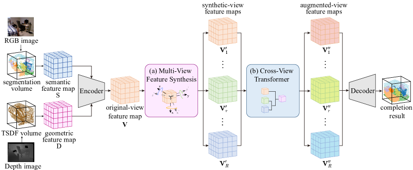
Figure 1: The overall architecture of CVSformer, which consists of Multi-View Feature Synthesis (MVFS) and Cross-View Transformer (CVTr). Based on a single-view RGB-D image, CVSformer computes the semantic and geometric feature maps, which are input into the MVFS (a) to achieve multiple synthetic-view feature maps. (b) CVTr takes input as the synthetic-view feature maps, yielding augmented-view feature maps for the final completion task.

In this paper, we propose Cross-View Synthesis Transformer (CVSformer), which consists of Multi-View Feature Synthesis (MVFS) and Cross-View Transformer (CVTr), as illustrated in Figure 1. CVSformer employs the basic 3D CNN to learn the visual feature map from RGB-D image. The original-view feature map contains the feature of each voxel, whose correlation with the adjacent voxels is captured from the original view. Next, MVFS controls the rotation of the 3D convolutional kernel, synthesizing the change of view direction and providing new object relationships. Here, we remark that 3D kernel’s view is an analogy with the camera’s view. It has a conceptual view direction to determines the center voxel’s spatial neighbors and their correlations. MVFS employs the kernels with different rotations to compute the synthetic-view feature maps, which capture the object relationships for each voxel from multiple views. Finally, all synthetic-view feature maps are input to CVTr, which conducts the cross-view fusion to establish the object relationships across multiple views. Based on the cross-view object relationships, CVTr enhances the synthetic-view feature maps, yielding the augmented-view feature maps for SSC.

We evaluate CVSformer on the public datasets for SSC, where we achieve the state-of-the-art results (i.e., 52.6 and 63.9 mIoUs on NYU [31] and NYUCAD [16] datasets).

2 Related work

Below, we mainly survey the literature on semantic scene completion and multi-view information fusion, which highly correlate to our method in modeling the geometric and semantic relationships between 3D objects.

2.1 Semantic Scene Completion

SSCNet [32] is a pioneering work that uses the deep network for semantic scene completion. It generates a complete 3D voxel representation of volumetric occupancy and semantic labels based on a single-view depth map. AICNet [19] employs an anisotropic convolution module to balance performance and computational cost. 3D sketch [5] introduces CVAE in the network to guide sketch generation. SISNet [1] lets the instance-completion and scene-completion promote mutually to obtain better completion results. CCPNet [40] has a cascaded architecture to achieve multi-scale 3D context and integrate local geometric details of the scene. SATNet [26] decomposes the semantic scene completion task into 2D semantic segmentation and 3D semantic scene completion, whose outputs are fused. ESSCNet [38] divides the input voxels into different groups and performs 3D sparse convolution separately. DDRNet [20] has a lightweight decomposition network to better fuse multi-scale features. FFNet [34] obtains augmented features by modeling the frequency domain correlation between RGB and depth data. ForkNet [36] generates new samples to assist the training process.

Currently, semantic scene completion relies on the input of single-view images, which provide little information to establish the connection between the occluded objects and their neighbors. In contrast, we propose the multi-view feature synthesis by controlling the rotated kernels, which are used to extract the geometric and semantic representations for modeling the multi-view object relationships.

2.2 Multi-View Information Fusion

Many works on multi-view information fusion have combined the features learned from bird’s eye view (BEV) and range view (RV) images. S3CNet [8] resorts to a set of bird’s eye views to assist scene reconstruction. VISTA [10] has dual cross-view spatial attention for fusing the multi-view image features. MVFuseNet [17] utilizes the sequential multi-view fusion network to learn the image features from the RV and BEV views. 3DMV [9] leverages a differentiable back-projection layer to incorporate the semantic features of RGB-D images. CVCNet [4] unifies BEV and RV, using a transformer to merge the two views. MVCNN [33] combines features of the same 3D shape from multiple perspectives. MV3D [6] uses the region-based representation to fuse multi-scale features deeply.

The above methods either fuse BEV and RV of objects or fuse features of RGB-D sequences. Yet, these methods are less applicable in considering the object relationships across various views, which offer critical object context for semantic scene completion. Our framework uses kernels with different rotations to synthesize multi-view features based on a single-view image. Furthermore, we feed the multi-view features into the cross-view transformer, which communicates the multi-view features and yields the augmented information of cross-view object relationships for the completion task.

3 Method Overview

We illustrate the overall architecture of CVSformer in Figure 1. At first, CVSformer takes the RGB image and the depth image as input. It projects the 2D semantic segmentation map of the RGB image into the voxelized segmentation volume [26], where each voxel is associated with a category. Meanwhile, CVSformer computes the voxelized TSDF volume based on the depth map, where each voxel in the TSDF volume has a signed distance to the nearest object surface. We perform 3D convolution on the segmentation and TSDF volumes, computing the 3D semantic feature and geometric maps ${\bf S},{\bf D}\in\mathbb{R}^{H\times W\times D\times C}$. Here, $H$, $W$, and $D$ represents the spatial resolutions along $x-$, $y-$, and $z-$axes. $C$ is the number of channels.

Next, CVSformer adds the 3D semantic feature and geometric maps ${\bf S}$ and ${\bf D}$ and passes them into an encoder architecture with multiple 3D convolutional layers for computing the original-view feature map ${\bf V}\in\mathbb{R}^{H\times W\times D\times C}$. Multi-View Feature Synthesis (MVFS) takes ${\bf V}$ as input. As illustrated in Figure 1(a), MVFS outputs a set of synthetic-view feature maps $\{{\bf V}^{\prime}_{r}\in\mathbb{R}^{H\times W\times D\times C}~{}|~{}r=1,...,R\}$. Each synthetic-view feature map is computed by convoluting a set of 3D kernels, which are rotated by a controllable degree (see Figure 3).

As illustrated in Figure 1(b), all of the synthetic-view feature maps are fed into Cross-View Transformer (CVTr). CVTr employs cross-view fusion to let the synthetic-view feature maps mutually augment each other in an all-for-one fashion. Rather than straightforwardly fusing multiple synthetic-view feature maps, where the high-dimensional feature represents each voxel, CVTr computes separate view-tokens for the synthetic-view feature maps (see Figure 4). Each view token is low-dimensional. It represents the complete information of the corresponding synthetic-view feature map. CVTr resorts to the view-tokens to enhance all of the synthetic-view feature maps, yielding a set of augmented-view feature maps $\{{\bf V}^{\prime\prime}_{r}\in\mathbb{R}^{H\times W\times D\times C}~{}|~{}r=1,...,R\}$.

Eventually, we concatenate the augmented-view feature maps, feeding them into a 3D-convolutional decoder. The decoder outputs the voxelized volume, where each voxel has a semantic category as the completion result.

4 Architecture of CVSformer

In this section, we provide more details of the critical components of CVSformer (i.e., Multi-View Feature Synthesis and Cross-View Transformer).

4.1 Multi-View Feature Synthesis

MVFS controls the rotation degree of 3D convolutional kernels. It convolutes the rotated kernels with the original-view feature map, yielding the synthetic-view feature maps.

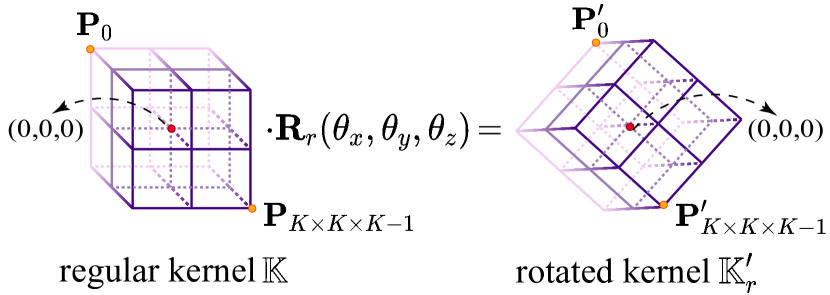
Figure 2: The illustration of controlling the degree to rotate a 3D convolutional kernel. We fix the kernel center during rotation.

Kernel Rotation   We explain how to control the rotation of the 3D convolutional kernel in Figure 2. In the left of Figure 2, we denote a $K\times K\times K$ 3D kernel as a set of 3D points $\mathbb{K}=\{{\bf P}_{k}\in\mathbb{R}^{3}~{}|~{}k=0,\cdots,K\times K\times K-1\}$. ${\bf P}_{k}$ contains $x-$, $y-$, and $z-$coordinates, which are computed as:

$$\left\{\begin{aligned} \begin{array}[]{l}{\bf x}_{k}=\frac{2(k\bmod K^{2}\bmod K)-{K-1}}{2}\vspace{2ex},\\ {\bf y}_{k}=\frac{2(k\bmod K^{2})-K({K-1})}{2K}\vspace{2ex},\\ {\bf z}_{k}=\frac{-2k+K^{2}({K-1})}{{2}{K^{2}}}\vspace{2ex},\\ {\bf P}_{k}=({\bf x}_{k},{\bf y}_{k},{\bf z}_{k}),\end{array}\end{aligned}\right.$$ (1)

where ${\bf P}_{0}=\left(-\frac{K-1}{2},-\frac{K-1}{2},\frac{K-1}{2}\right)$, ${\bf P}_{\frac{K\times K\times K-1}{2}}=\left(0,0,0\right)$, and ${\bf P}_{K\times K\times K-1}=\left(\frac{K-1}{2},\frac{K-1}{2},-\frac{K-1}{2}\right)$ represent the top-left, center, and bottom-right vertexes of the 3D kernel $\mathbb{K}$, respectively. And mod means the remainder operator with a left-to-right precedence.

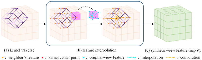
Figure 3: The architecture of MVFS. It consists of two parts: Kernel Rotation and Interpolation. We calculate the synthetic-view feature maps by convoluting the different rotated kernels to the feature map of the original view.

As illustrated in the right of Figure 2, we rotate the kernel $\mathbb{K}$ around $x-$, $y-$, and $z-$axes centered on ${\bf P}_{\frac{K\times K\times K-1}{2}}$. For this purpose, we prepare a set of hybrid rotation matrices $\{{\bf R}_{r}\left(\theta_{x},\theta_{{y}},\theta_{{z}}\right)\in\mathbb{R}^{3\times 3}~{}|~{}r=1,...,R\}$. We compute the $r^{th}$ rotation matrix ${\bf R}_{r}\left(\theta_{x},\theta_{{y}},\theta_{{z}}\right)$ as:

$$\left\{\begin{aligned} \begin{array}[]{l}{\bf R}_{r}\left({\theta}_{{x}}\right)=\left[\begin{array}[]{ccc}-\cos\theta_{{x}}&\sin\theta_{{x}}&0\\ -\sin\theta_{{x}}&-\cos\theta_{{x}}&0\\ 0&0&1\end{array}\right]\vspace{2ex},\\ {\bf R}_{r}\left(\theta_{{y}}\right)=\left[\begin{array}[]{ccc}\hskip 8.00003pt\cos\theta_{y}&\hskip 5.0pt0&\hskip 6.00006pt\sin\theta_{y}\\ 0&\hskip 5.0pt1&0\\ -\sin\theta_{y}&\hskip 5.0pt0&\hskip 6.00006pt\cos\theta_{y}\end{array}\right]\vspace{2ex},\\ {\bf R}_{r}\left(\theta_{{z}}\right)=\left[\begin{array}[]{ccc}\hskip 1.00006pt1&0&0\\ \hskip 1.00006pt0&-\cos\theta_{z}&\sin\theta_{z}\\ \hskip 1.00006pt0&-\sin\theta_{z}&-\cos\theta_{z}\end{array}\right]\vspace{2ex},\\ {\bf R}_{r}\left(\theta_{x},\theta_{{y}},\theta_{{z}}\right)={\bf R}_{r}\left(\theta_{x}\right)\cdot{\bf R}_{r}\left(\theta_{{y}}\right)\cdot{\bf R}_{r}\left(\theta_{{z}}\right),\end{array}\end{aligned}\right.$$ (2)

where $\theta_{x}$, $\theta_{y}$, $\theta_{z}$ represent the rotation degrees around the $x-$, $y-$, and $z-$axes, respectively. We use ${\bf R}_{r}\left(\theta_{x},\theta_{{y}},\theta_{{z}}\right)$ to rotate the vertexes in the kernel $\mathbb{K}$ as:

$${\bf P}^{\prime}_{r,k}={\bf P}_{k}\cdot{\bf R}_{r}\left(\theta_{x},\theta_{y},\theta_{z}\right),$$ (3)

where we form a new kernel $\mathbb{K}^{\prime}_{r}=\{{\bf P}^{\prime}_{r,k}\in\mathbb{R}^{3}~{}|~{}k=0,\cdots,K\times K\times K-1\}$ with a rotated view.

Feature Interpolation for Rotated Kernel   We convolute the rotated 3D kernels with the original-view feature map ${\bf V}\in\mathbb{R}^{H\times W\times D\times C}$ to compute a set of synthetic-view feature maps $\{{\bf V}^{\prime}_{r}\in\mathbb{R}^{H\times W\times D\times C}~{}|~{}r=1,...,R\}$. We provide the details of using the rotated kernel $\mathbb{K}^{\prime}_{r}$ to compute the synthetic-view feature map ${\bf V}^{\prime}_{r}$ in Figure 3. During the convolution, we traverse the center of the rotated kernel $\mathbb{K}^{\prime}_{r}$ along $x-$, $y-$, and $z-$axes of the original-view feature map ${\bf V}$ (see Figure 3(a)).

Given the $i^{th}$ vertex ${\bf v}_{i}$ of ${\bf V}$ (see Figure 3(b)), which overlaps with the center of the rotated kernel $\mathbb{K}^{\prime}_{r}$, we achieve $K\times K\times K$ neighbors of ${\bf v}_{i}$. We denote the neighbors as a set of 3D points $\{\widetilde{\bf v}_{i,k}\in\mathbb{R}^{3}~{}|~{}k=1,...,K\times K\times K-1\}$, where we compute $\widetilde{\bf v}_{i,k}$ as:

$$\widetilde{\bf v}_{i,k}={\bf v}_{i}+{\bf P}^{\prime}_{r,k}.$$ (4)

Different from any vertex of the feature map ${\bf V}$, the feature located at the vertex $\widetilde{\bf v}_{i,k}$ may be unavailable. To enable a valid convolution on the set $\mathbb{N}\left({\bf v}_{i}\right)$, we resort to the feature interpolation to approximate the feature $\widetilde{\bf V}_{i,k}\in\mathbb{R}^{C}$ of the vertex $\widetilde{\bf v}_{i,k}$. The interpolation uses the vertexes of the unit cube, where the $\widetilde{\bf v}_{i,k}$ resides, to compute $\widetilde{\bf V}_{i,k}$ as:

$$\widetilde{\bf V}_{i,k}=\sum^{K\times K\times K-1}_{k=0}(1-|{\bf v}_{j}-\widetilde{\bf v}_{i,k}|)\cdot{\bf V}_{j},$$ (5)

$$~{}~{}~{}~{}~{}s.t.~{}~{}({\bf v}_{j}-\widetilde{\bf v}_{i,k})^{\top}({\bf v}_{j}-\widetilde{\bf v}_{i,k})\leq 1.$$

Here, ${\bf v}_{j}$ is the $j^{th}$ vertex of the feature map ${\bf V}$. ${\bf v}_{j}$ is associated with the feature ${\bf V}_{j}\in\mathbb{R}^{C}$. The feature interpolation yields a set of features $\mathbb{N}\left({\bf v}_{i}\right)=\{\widetilde{\bf V}_{i,k}\in\mathbb{R}^{C}~{}|~{}k=1,...,K\times K\times K-1\}$ centered at the vertex ${\bf v}_{i}$. We convolute the rotated kernel $\mathbb{K}^{\prime}_{r}$ with the feature set $\mathbb{N}\left({\bf v}_{i}\right)$ as:

$${\bf V}^{\prime}_{r,i}=\sum^{K\times K\times K-1}_{k=0}{\bf w}^{\prime}_{r,k}\cdot\widetilde{\bf V}_{i,k},$$ (6)

where ${\bf w}^{\prime}_{r,k}$ is the weight associated with the vertex ${\bf P}^{\prime}_{r,k}$ of the rotated kernel $\mathbb{K}^{\prime}_{r}$. ${\bf V}^{\prime}_{r,i}\in\mathbb{R}^{C}$ represents the feature of the vertex ${\bf v}_{i}$ of the synthetic-view feature map ${\bf V}^{\prime}_{r}$.

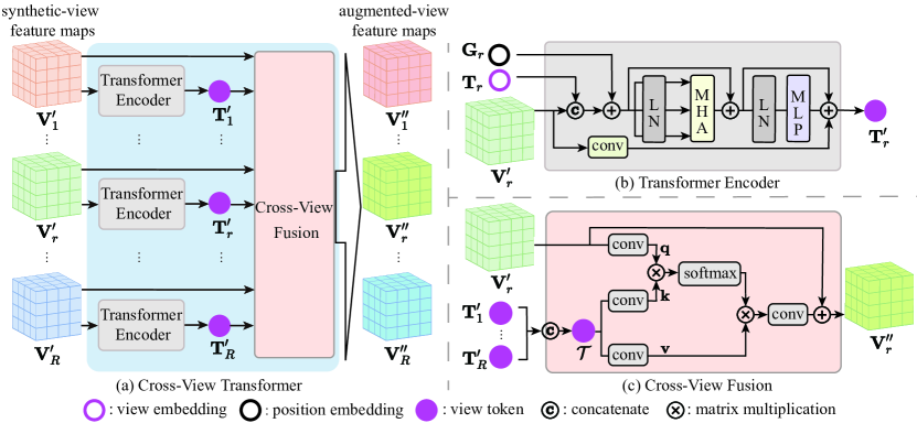
Figure 4: (a) The overall architecture of CVTr. CVTr has several transformer encoders (b) for computing a low-dimensional view token. All view tokens are used by the cross-view fusion (c) for computing the augmented-view feature map.

4.2 Cross-View Transformer

We illustrate the architecture of CVTr in Figure 4(a). We elaborate on the key modules of CVTr, i.e., transformer encoder and cross-view fusion in Figure 4(b–c).

Transformer Encoder   We illustrate a transformer encoder in Figure 4(b). We input the synthetic-view feature map ${\bf V}^{\prime}_{r}\in\mathbb{R}^{H\times W\times D\times C}$, the learnable view embedding ${\bf T}_{r}\in\mathbb{R}^{M\times C}$, and the learnable position embedding ${\bf G}_{r}\in\mathbb{R}^{(M+H\times W\times D)\times C}$ into the $r^{th}$ encoder. $M$ represents the resolution of the view embedding. The encoder outputs a low-dimensional view token ${\bf T}^{\prime}_{r}\in\mathbb{R}^{M\times C}$ for representing the entire ${\bf V}^{\prime}_{r}$ with a higher dimension.

The encoder uses convolution to transform the synthetic-view feature map ${\bf V}^{\prime}_{r}$, which is added to the view token ${\bf T}^{\prime}_{r}$. This step is critical to the completion task based on the voxelized structure. It helps the view token ${\bf T}^{\prime}_{r}$ with lower dimension to capture the underlying configuration of voxels.

The spatial dimension of the view embedding ${\bf T}_{r}$ is lower than the synthetic-view feature map ${\bf V}^{\prime}_{r}$ (i.e., $M<H\times W\times D$). By compressing the spatial dimension of ${\bf T}_{r}$, we drive the ${\bf T}_{r}$ to focus on the global semantic meaning of ${\bf V}^{\prime}_{r}$, which is injected into the view token ${\bf T}^{\prime}_{r}$.

The position embedding ${\bf G}_{r}$ are jointly learned with the view embedding ${\bf T}_{r}$ and the synthetic-view feature map ${\bf V}^{\prime}_{r}$. Thus, ${\bf G}_{r}$ can be regarded as a complementary structure, which stores richer geometric information than the view embedding ${\bf T}_{r}$. We also inject the geometric information of ${\bf G}_{r}$ into the view token ${\bf T}^{\prime}_{r}$.

Cross-View Fusion   For all views, we use different transformer encoders to compute the view tokens $\{{\bf T}^{\prime}_{r}\in\mathbb{R}^{M\times C}~{}|~{}r=1,...,R\}$. The cross-view fusion harnesses the view tokens to enhance the synthetic-view feature maps.

We provide more details of cross-view fusion in Figure 4(c). First, we concatenate all of the view tokens, forming an overall token $\mathcal{T}\in\mathbb{R}^{M\times R\times C}$ with hybrid information across different views. Next, we establish cross attention between the overall token $\mathcal{T}$ and the synthetic-view feature map ${\bf V}^{\prime}_{r}$. With the cross-view information of $\mathcal{T}$, the cross attention enhances ${\bf V}^{\prime}_{r}$ and computes the augmented-view feature map ${\bf V}^{\prime\prime}_{r}\in\mathbb{R}^{H\times W\times D\times C}$:

$$\left\{\begin{aligned} \begin{array}[]{l}{\bf q}=conv({{\bf V}^{\prime}_{r}}),~{}{\bf k}=conv({\mathcal{T}}),~{}{\bf v}=conv({\mathcal{T}})\vspace{2ex},\\ {\bf A}={\bf v}^{\top}\cdot softmax({\bf k}\cdot{\bf q}^{\top})\vspace{2ex},\\ {\bf V}^{\prime\prime}_{r}={\bf V}^{\prime}_{r}+conv({\bf A}^{\top}).\end{array}\end{aligned}\right.$$ (7)

To simplify the notations above, we omit the subscripts of the intermediate variables ${\bf k},{\bf v}\in\mathbb{R}^{M\times R\times C}$ and ${\bf q},{\bf A}\in\mathbb{R}^{H\times W\times D\times C}$. CVTr produces a set of augmented-view feature maps $\{{\bf V}^{\prime\prime}_{r}\in\mathbb{R}^{H\times W\times D\times C}~{}|~{}r=1,...,R\}$, which are added together and passed to a 3D convolutional decoder for predicting the complete scene.

5 Experiments

5.1 Implementation Details

We use PyTorch to construct CVSformer. Before training CVSformer, we pre-train DeepLabv3 [3] for 1,000 epochs to segment the RGB image. Below, we fix the optimized network parameters of DeepLabv3.

The voxel-wise cross-entropy loss supervises the scene completion task. We employ SGD solver to optimize CVSformer with a momentum of 0.9 and a weight decay of 0.0005. We set the initial learning rate to 0.05, which is adjusted by the poly scheduler. We train the network for $500$ epoches, where each min-batch contains $16$ samples.

The spatial resolution of the segmentation and TSDF volumes are $60\times 36\times 60$, and the resolution of original-view feature map is $15\times 9\times 15$. In MVFS, the rotated kernels are $3\times 3\times 3$. We empirically choose the rotation degrees along $x-$, $y-$, and $z-$axes from the set $\{0^{\circ},45^{\circ},90^{\circ},135^{\circ}\}$. To simplify the experiment, we empirically rotate the 3D kernel along $x-$axis. In CVTr, we set the spatial dimension $M\!=\!75$ of the view token as default.

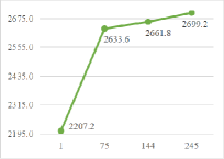
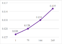
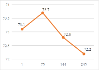
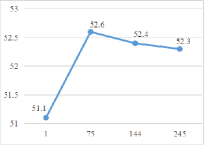
(a) GPU Memory	(b) Testing Time	(c) IoU(%)	(d) mIoU(%)

Figure 5: Sensitivities of GPU memory in MB (a), testing time per image in seconds (b), IoU (c), and mIoU (d) to the spatial resolution of view token. The performances are evaluated on NYU dataset.

5.2 Experimental Datasets

Datasets   We compare CVSformer with state-of-the-art methods on the real NYU [31] and NYUCAD [16] datasets. They both provide 1,449 pairs of RGB-D images, and there are $795$/$654$ pairs for training and test. We use the 3D annotation provided in [29] for the network training.

Evaluation Metrics   We report the accuracies of scene completion (SC) and semantic scene completion (SSC) on different datasets. We use the recall, precision, and voxel-wise intersection-over-union (IoU) on the occluded voxels to measure the accuracy of SC. To calculate the accuracy of SSC, we report IoUs on different semantic categories, which are averaged to achieve mean IoU.

5.3 Internal Study of CVSformer

We use NYU [31] for examining the effectiveness of CVSformer and its key components (i.e., MVFS and CVTr).

Spatial Resolution of View Tokens   We change the spatial resolution of view tokens and examine the effect on the computational overheads (i.e., GPU memory and testing time in Figure 5(a–b)) and the performances (i.e., SC-IoU and SSC-mIoU in Figure 5(c–d)). We choose the spatial resolution from the set $\{1,75,144,245\}$, which corresponds to $\{1\times 1\times 1,5\times 3\times 5,6\times 4\times 6,7\times 5\times 7\}$ voxelized volumes, respectively. A higher resolution (e.g., $M=75$) allows view tokens to contain richer information of voxelized configuration, semantic meaning, and geometric relationship between objects. However, the view tokens with too high resolutions (e.g., $M=144$ and $245$) inevitably require more computation. They contain a too complex mixture of information. These view tokens are used by the cross-view fusion, where the complex information distracts the specific information of each view’s feature map. Thus, they degrade the performances.

Different Strategies of Learning View Tokens   In Table 1, we experiment with different strategies for learning view tokens. As reported in the first and second rows, we use the regular 3D convolution and self-attention to learn the view tokens, respectively, achieving (72.6% IoU, 51.8% mIoU) and (72.7% IoU, 52.0% mIoU). Note that self-attention slightly outperforms the regular 3D convolution because it is good at capturing long-range dependencies of the whole scene. Yet, it eliminates the configuration of the voxelized structure, which is respected by the regular 3D convolution. The importance of respecting the voxelized format is evidenced by the performance improvement up to (73.7% IoU, 52.6% mIoU) when we combine 3d convolution and self-attention for learning the view tokens.

View Token	IoU(%)	mIoU(%)
convolution	72.6	51.8
self-attention	72.7	52.0
convolution + self-attention	73.7	52.6

Table 1: Various strategies for learning view tokens. The performances are evaluated on NYU dataset.

Sensitivity to View Number in MVFS   We experiment with changing the number of views, where each view is associated with a rotation degree in the set $\{0^{\circ},45^{\circ},90^{\circ},135^{\circ}\}$. Different views yield the corresponding synthetic-view feature maps. We report the performances in Table 2. We find that more views saturate IoU sensitive to the object occupancies in the voxels. Comparably, multiple synthetic-view feature maps are used by CVTr to capture cross-view object relationships for comprehensively representing the semantic correlation between objects. Compared to the single view (i.e., $0^{\circ}$), more views improve mIoU up to 52.6%, which requires differentiating the semantic object categories. More detailed discussion of MVFS can be found in the supplementary material.

Rotation Degrees	IoU(%)	mIoU(%)
$0^{\circ}$	72.9	51.3
$\{0^{\circ},45^{\circ}\}$	73.8	52.1
$\{0^{\circ},45^{\circ},90^{\circ}\}$	73.5	52.0
$\{0^{\circ},45^{\circ},90^{\circ},135^{\circ}\}$	73.7	52.6

Table 2: Various number of views in MVFS. The performances are evaluated on NYU dataset.

Different Fusion Schemes in CVTr   In Table 3, we compare different alternatives of cross-view fusion. We concatenate all synthetic-view feature maps fed into self-attention for computing an augmented-view feature map (see “all fusion”). This scheme yields the performances of (73.0% IoU, 52.3% mIoU).

Fusion Scheme	IoU(%)	mIoU(%)
all fusion	73.0	52.3
all-for-one w.r.t. feature maps	72.9	51.6
all-for-one w.r.t. tokens	73.7	52.6

Table 3: Various fusion schemes in CVTr. The performances are evaluated on NYU dataset.

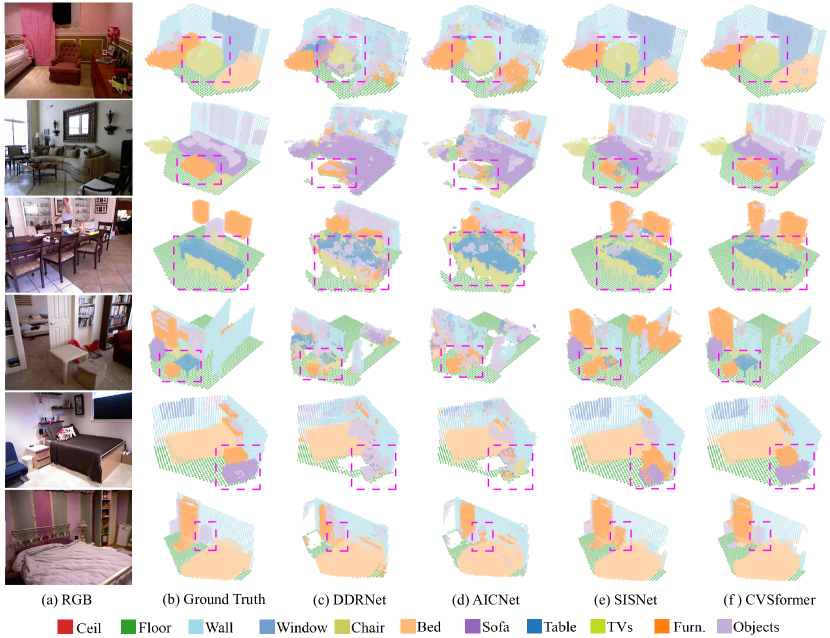
Figure 6: Completion results of different methods. The examples are taken from the test set of NYU.

In the second scheme (see “all-for-one w.r.t. feature maps”), we concatenate all synthetic-view feature maps as the key and value of cross attention, which enhances each synthetic-view feature map. This scheme yields performances (72.9% IoU, 51.6% mIoU) worse than the first scheme. It evidences that high-dimensional synthetic-view feature maps contain redundant information for distracting the information fusion between multiple views.

Our cross-view fusion (see “all-for-one w.r.t. tokens”) employs the concatenated view tokens learned by the transformer encoders as the key and value for feature enhancement. The cross-view fusion refines the semantic and geometric information contained in the relatively low-dimensional view tokens, outperforming other alternatives.

MVFS	CVTr	IoU(%)	mIoU(%)
		72.9	51.3
✓		73.2	51.8
✓	✓	73.7	52.6

Table 4: Ablation study on MVFS and CVTr. The performances are evaluated on NYU dataset.

Method	SC			SSC
	prec.	recall	IoU	ceil.	floor	wall	win.	chair	bed	sofa	table	tvs	furn.	objs.	avg.
SISNet(instance) [1]	92.1	83.8	78.2	54.7	93.8	53.2	41.9	43.6	66.2	61.4	38.1	29.8	53.9	40.3	52.4
SSCNet [32]	57.0	94.5	55.1	15.1	94.7	24.4	0.0	12.6	32.1	35.0	13.0	7.8	27.1	10.1	24.7
DDRNet [20]	71.5	80.8	61.0	21.1	92.2	33.5	6.8	14.8	48.3	42.3	13.2	13.9	35.3	13.2	30.4
AICNet [19]	62.4	91.8	59.2	23.2	90.8	32.3	14.8	18.2	51.1	44.8	15.2	22.4	38.3	15.7	33.3
SATNet [26]	67.3	85.8	60.6	17.3	92.1	28.0	16.6	19.3	57.5	53.8	17.2	18.5	38.4	18.9	34.4
CCPNet [40]	74.2	90.8	63.5	23.5	96.3	35.7	20.2	25.8	61.4	56.1	18.1	28.1	37.8	20.1	38.5
Sketch [5]	85.0	81.6	71.3	43.1	93.6	40.5	24.3	30.0	57.1	49.3	29.2	14.3	42.5	28.6	41.1
SemanticFu [14]	86.6	82.4	73.1	45.4	92.3	41.1	25.6	32.6	58.3	49.8	30.5	17.1	44.1	33.9	42.8
FFNet [34]	89.3	78.5	71.8	44.0	93.7	41.5	29.3	36.2	59.0	51.1	28.9	26.5	45.0	32.6	44.4
SISNet(voxel) [1]	88.7	77.7	70.8	46.8	93.4	42.0	32.4	36.0	61.1	55.8	28.2	27.6	45.7	32.9	45.6
PCANet [22]	89.5	87.5	78.9	44.3	94.5	50.1	30.7	41.8	68.5	56.4	32.6	29.9	53.6	35.4	48.9
CVSformer	87.7	82.1	73.7	46.3	94.3	43.5	42.8	46.2	67.7	66.0	39.2	43.2	53.9	35.0	52.6

Table 5: We compare CVSformer with state-of-the-art methods on the test set of NYU.

Method	SC			SSC
	prec.	recall	IoU	ceil.	floor	wall	win.	chair	bed	sofa	table	tvs	furn.	objs.	avg.
SISNet(instance) [1]	94.1	91.2	86.3	63.4	94.4	67.2	52.4	59.2	77.9	71.1	51.8	46.2	65.8	48.8	63.5
SSCNet [32]	75.4	96.3	73.2	32.5	92.6	40.2	8.9	33.9	57.0	59.5	28.3	8.1	44.8	25.1	40.0
DDRNet [20]	88.7	88.5	79.4	54.1	91.5	56.4	14.9	37.0	55.7	51.0	28.8	9.2	44.1	27.8	42.8
AICNet [19]	88.2	90.3	80.5	53.0	91.2	57.2	20.2	44.6	58.4	56.2	36.2	9.7	47.1	30.4	45.8
CCPNet [40]	91.3	92.6	82.4	56.2	94.6	58.7	35.1	44.8	68.6	65.3	37.6	35.5	53.1	35.2	53.2
Sketch [5]	90.6	92.2	84.2	59.7	94.3	64.3	32.6	51.7	72.0	68.7	45.9	19.0	60.5	38.5	55.2
SemanticFu [14]	88.7	92.5	84.8	54.5	94.8	63.3	29.3	50.9	73.6	70.9	56.4	31.7	61.3	42.0	57.2
FFNet [34]	94.8	90.3	85.5	62.7	94.9	67.9	35.2	52.0	74.8	69.9	47.9	27.9	62.7	35.1	57.4
SISNet(voxel) [1]	92.0	89.3	82.8	62.0	94.1	63.3	43.5	50.8	73.3	63.5	42.2	40.6	58.2	39.7	57.4
PCANet [22]	92.1	91.8	84.3	54.8	93.1	62.8	44.3	52.3	75.6	70.2	46.9	44.8	65.3	45.8	59.6
CVSformer	94.0	91.0	86.0	65.6	94.2	60.6	54.7	60.4	81.8	71.3	49.8	55.5	65.5	43.5	63.9

Table 6: We compare CVSformer with state-of-the-art methods on the test set of NYUCAD.

Analysis of Network Components   In Table 4, we examine the effectiveness of the critical components (i.e., MVFS and CVTr), by removing one or more components from the completion network. In the first row, we use the baseline network without decoration, which employs the primary 3D convolution to learn the original-view feature map from RGB-D image for semantic scene completion. This method produces (72.9% IoU, 51.3% mIoU).

We add MVFS to the network (see the second row) for computing multiple synthetic-view feature maps, which are concatenated for regressing the final result. MVFS helps to improve performance (73.2% IoU, 51.8% mIoU), demonstrating the necessity of multi-view information.

Next, we combine MVFS and CVTr (see the third row) to form the entire model. Here, we fuse the multi-view information to compute the augmented-view feature maps, further improving performance (73.7 IoU%, 52.6% mIoU). This result demonstrates that the trivial concatenation of synthetic-view feature maps in the second alternative is less effective in modeling the cross-view object relationship.

5.4 Comparisons with State-of-the-Art Methods

Below, we compare CVSformer with state-of-the-art methods on NYU [31] and NYUCAD [16] datasets in Tables 5 and 6.

We compare CVSformer with the completion methods that rely on voxel-wise annotations for the network training. Here, CVSformer outperforms the current methods (e.g., Sketch [5] and SISNet(voxel) [1]) by a remarkable margin. In Figure 6, CVSformer achieves the visualized results better than the competitive methods. More results please refer to supplementary materials.

The latest SISNet(instance) [1] takes advantage of the instance-wise annotations, which provide more substantial supervision than the voxel-wise annotations for the network training. It achieves remarkable performances, i.e., (78.2% IoU, 52.4% mIoU) on NYU and (86.3% IoU, 63.5% mIoU) on NYUCAD. CVSformer still outperforms SISNet(instance) [1] by only requiring voxel-wise annotations on NYU and NYUCAD.

We also evaluate the computation overhead of CVSformer with other methods, in terms of GPU memory, running time, and model capacity. Compared to AICNet (3413M, 0.23s/scene, 0.72M), DDRNet (3007M, 0.14s/scene, 0.20M), and SISNet (3750M, 0.18s/scene, 0.57M), CVSformer (2633M, 0.13s/scene, 0.41M) requires reasonable computation.

6 Conclusion

The latest progress in semantic scene completion benefits from deep neural networks to learn the geometric and semantic features of 3D objects. In this paper, we propose CVSformer that understands cross-view object relationships for semantic scene completion. CVSformer controls kernels with different rotations to learn multi-view object relationships. Furthermore, we utilize a cross-view fusion to exchange information across different views, thus capturing the cross-view object relationships. CVSformer achieves state-of-the-art performances on public datasets. In the future, we plan to explore how to use CVSformer for other 3D object recognition tasks.

References

- [1] Yingjie Cai, Xuesong Chen, Chao Zhang, Kwan-Yee Lin, Xiaogang Wang, and Hongsheng Li. Semantic scene completion via integrating instances and scene in-the-loop. In Proceedings of the IEEE/CVF Conference on Computer Vision and Pattern Recognition, pages 324–333, 2021.
- [2] Anh-Quan Cao and Raoul de Charette. Monoscene: Monocular 3d semantic scene completion. In Proceedings of the IEEE/CVF Conference on Computer Vision and Pattern Recognition, pages 3991–4001, 2022.
- [3] Liang-Chieh Chen, George Papandreou, Iasonas Kokkinos, Kevin Murphy, and Alan L Yuille. Deeplab: Semantic image segmentation with deep convolutional nets, atrous convolution, and fully connected crfs. IEEE transactions on pattern analysis and machine intelligence, 40(4):834–848, 2017.
- [4] Qi Chen, Lin Sun, Ernest Cheung, and Alan L Yuille. Every view counts: Cross-view consistency in 3d object detection with hybrid-cylindrical-spherical voxelization. Advances in Neural Information Processing Systems, 33:21224–21235, 2020.
- [5] Xiaokang Chen, Kwan-Yee Lin, Chen Qian, Gang Zeng, and Hongsheng Li. 3d sketch-aware semantic scene completion via semi-supervised structure prior. In Proceedings of the IEEE/CVF Conference on Computer Vision and Pattern Recognition, pages 4193–4202, 2020.
- [6] Xiaozhi Chen, Huimin Ma, Ji Wan, Bo Li, and Tian Xia. Multi-view 3d object detection network for autonomous driving. In Proceedings of the IEEE conference on Computer Vision and Pattern Recognition, pages 1907–1915, 2017.
- [7] Yueh-Tung Chen, Martin Garbade, and Juergen Gall. 3d semantic scene completion from a single depth image using adversarial training. In 2019 IEEE International Conference on Image Processing (ICIP), pages 1835–1839. IEEE, 2019.
- [8] Ran Cheng, Christopher Agia, Yuan Ren, Xinhai Li, and Liu Bingbing. S3cnet: A sparse semantic scene completion network for lidar point clouds. In Conference on Robot Learning, pages 2148–2161. PMLR, 2021.
- [9] Angela Dai and Matthias Nießner. 3dmv: Joint 3d-multi-view prediction for 3d semantic scene segmentation. In Proceedings of the European Conference on Computer Vision (ECCV), pages 452–468, 2018.
- [10] Shengheng Deng, Zhihao Liang, Lin Sun, and Kui Jia. Vista: Boosting 3d object detection via dual cross-view spatial attention. In Proceedings of the IEEE/CVF Conference on Computer Vision and Pattern Recognition, pages 8448–8457, 2022.
- [11] Aloisio Dourado, Teofilo Emidio de Campos, Hansung Kim, and Adrian Hilton. Edgenet: Semantic scene completion from rgb-d images. arXiv preprint arXiv:1908.02893, 1, 2019.
- [12] Aloisio Dourado, Frederico Guth, and Teofilo de Campos. Data augmented 3d semantic scene completion with 2d segmentation priors. In Proceedings of the IEEE/CVF Winter Conference on Applications of Computer Vision, pages 3781–3790, 2022.
- [13] Aloisio Dourado, Hansung Kim, Teofilo E de Campos, and Adrian Hilton. Semantic scene completion from a single 360-degree image and depth map. In VISIGRAPP (5: VISAPP), pages 36–46, 2020.
- [14] Ruochong Fu, Hang Wu, Mengxiang Hao, and Yubin Miao. Semantic scene completion through multi-level feature fusion. In 2022 IEEE/RSJ International Conference on Intelligent Robots and Systems (IROS), pages 8399–8406. IEEE, 2022.
- [15] Martin Garbade, Yueh-Tung Chen, Johann Sawatzky, and Juergen Gall. Two stream 3d semantic scene completion. In Proceedings of the IEEE/CVF Conference on Computer Vision and Pattern Recognition Workshops, pages 0–0, 2019.
- [16] Yu-Xiao Guo and Xin Tong. View-volume network for semantic scene completion from a single depth image. arXiv preprint arXiv:1806.05361, 2018.
- [17] Ankit Laddha, Shivam Gautam, Stefan Palombo, Shreyash Pandey, and Carlos Vallespi-Gonzalez. Mvfusenet: Improving end-to-end object detection and motion forecasting through multi-view fusion of lidar data. In Proceedings of the IEEE/CVF Conference on Computer Vision and Pattern Recognition, pages 2865–2874, 2021.
- [18] Jie Li, Laiyan Ding, and Rui Huang. Imenet: Joint 3d semantic scene completion and 2d semantic segmentation through iterative mutual enhancement. arXiv preprint arXiv:2106.15413, 2021.
- [19] Jie Li, Kai Han, Peng Wang, Yu Liu, and Xia Yuan. Anisotropic convolutional networks for 3d semantic scene completion. In Proceedings of the IEEE/CVF Conference on Computer Vision and Pattern Recognition, pages 3351–3359, 2020.
- [20] Jie Li, Yu Liu, Dong Gong, Qinfeng Shi, Xia Yuan, Chunxia Zhao, and Ian Reid. Rgbd based dimensional decomposition residual network for 3d semantic scene completion. In Proceedings of the IEEE/CVF Conference on Computer Vision and Pattern Recognition, pages 7693–7702, 2019.
- [21] Jie Li, Yu Liu, Xia Yuan, Chunxia Zhao, Roland Siegwart, Ian Reid, and Cesar Cadena. Depth based semantic scene completion with position importance aware loss. IEEE Robotics and Automation Letters, 5(1):219–226, 2019.
- [22] Jie Li, Qi Song, Xiaohu Yan, Yongquan Chen, and Rui Huang. From front to rear: 3d semantic scene completion through planar convolution and attention-based network. IEEE Transactions on Multimedia, 2023.
- [23] Siqi Li, Changqing Zou, Yipeng Li, Xibin Zhao, and Yue Gao. Attention-based multi-modal fusion network for semantic scene completion. In Proceedings of the AAAI Conference on Artificial Intelligence, volume 34, pages 11402–11409, 2020.
- [24] Yiming Li, Zhiding Yu, Christopher Choy, Chaowei Xiao, Jose M Alvarez, Sanja Fidler, Chen Feng, and Anima Anandkumar. Voxformer: Sparse voxel transformer for camera-based 3d semantic scene completion. arXiv preprint arXiv:2302.12251, 2023.
- [25] Yiqing Liang, Boyuan Chen, and Shuran Song. Sscnav: Confidence-aware semantic scene completion for visual semantic navigation. In 2021 IEEE international conference on robotics and automation (ICRA), pages 13194–13200. IEEE, 2021.
- [26] Shice Liu, Yu Hu, Yiming Zeng, Qiankun Tang, Beibei Jin, Yinhe Han, and Xiaowei Li. See and think: Disentangling semantic scene completion. Advances in Neural Information Processing Systems, 31, 2018.
- [27] Yu Liu, Jie Li, Qingsen Yan, Xia Yuan, Chunxia Zhao, Ian Reid, and Cesar Cadena. 3d gated recurrent fusion for semantic scene completion. arXiv preprint arXiv:2002.07269, 2020.
- [28] Ruihang Miao, Weizhou Liu, Mingrui Chen, Zheng Gong, Weixin Xu, Chen Hu, and Shuchang Zhou. Occdepth: A depth-aware method for 3d semantic scene completion. arXiv preprint arXiv:2302.13540, 2023.
- [29] Jason Rock, Tanmay Gupta, Justin Thorsen, JunYoung Gwak, Daeyun Shin, and Derek Hoiem. Completing 3d object shape from one depth image. In Proceedings of the IEEE conference on computer vision and pattern recognition, pages 2484–2493, 2015.
- [30] Luis Roldao, Raoul de Charette, and Anne Verroust-Blondet. Lmscnet: Lightweight multiscale 3d semantic completion. In 2020 International Conference on 3D Vision (3DV), pages 111–119. IEEE, 2020.
- [31] Nathan Silberman, Derek Hoiem, Pushmeet Kohli, and Rob Fergus. Indoor segmentation and support inference from rgbd images. In European conference on computer vision, pages 746–760. Springer, 2012.
- [32] Shuran Song, Fisher Yu, Andy Zeng, Angel X Chang, Manolis Savva, and Thomas Funkhouser. Semantic scene completion from a single depth image. In Proceedings of the IEEE conference on computer vision and pattern recognition, pages 1746–1754, 2017.
- [33] Hang Su, Subhransu Maji, Evangelos Kalogerakis, and Erik Learned-Miller. Multi-view convolutional neural networks for 3d shape recognition. In Proceedings of the IEEE international conference on computer vision, pages 945–953, 2015.
- [34] Xuzhi Wang, Di Lin, and Liang Wan. Ffnet: Frequency fusion network for semantic scene completion. In Proceedings of the AAAI Conference on Artificial Intelligence, volume 36, pages 2550–2557, 2022.
- [35] Yida Wang, David Joseph Tan, Nassir Navab, and Federico Tombari. Adversarial semantic scene completion from a single depth image. In 2018 International Conference on 3D Vision (3DV), pages 426–434. IEEE, 2018.
- [36] Yida Wang, David Joseph Tan, Nassir Navab, and Federico Tombari. Forknet: Multi-branch volumetric semantic completion from a single depth image. In Proceedings of the IEEE/CVF International Conference on Computer Vision, pages 8608–8617, 2019.
- [37] Xinyi Ying, Longguang Wang, Yingqian Wang, Weidong Sheng, Wei An, and Yulan Guo. Deformable 3d convolution for video super-resolution. IEEE Signal Processing Letters, 27:1500–1504, 2020.
- [38] Jiahui Zhang, Hao Zhao, Anbang Yao, Yurong Chen, Li Zhang, and Hongen Liao. Efficient semantic scene completion network with spatial group convolution. In Proceedings of the European Conference on Computer Vision (ECCV), pages 733–749, 2018.
- [39] Liang Zhang, Le Wang, Xiangdong Zhang, Peiyi Shen, Mohammed Bennamoun, Guangming Zhu, Syed Afaq Ali Shah, and Juan Song. Semantic scene completion with dense crf from a single depth image. Neurocomputing, 318:182–195, 2018.
- [40] Pingping Zhang, Wei Liu, Yinjie Lei, Huchuan Lu, and Xiaoyun Yang. Cascaded context pyramid for full-resolution 3d semantic scene completion. In Proceedings of the IEEE/CVF International Conference on Computer Vision, pages 7801–7810, 2019.