A Novel Truncated Norm Regularization Method for Multi-channel Color Image Denoising

Abstract

Due to the high flexibility and remarkable performance, low-rank approximation methods has been widely studied for color image denoising. However, those methods mostly ignore either the cross-channel difference or the spatial variation of noise, which limits their capacity in real world color image denoising. To overcome those drawbacks, this paper is proposed to denoise color images with a double-weighted truncated nuclear norm minus truncated Frobenius norm minimization (DtNFM) method. Through exploiting the nonlocal self-similarity of the noisy image, the similar structures are gathered and a series of similar patch matrices are constructed. For each group, the DtNFM model is conducted for estimating its denoised version. The denoised image would be obtained by concatenating all the denoised patch matrices. The proposed DtNFM model has two merits. First, it models and utilizes both the cross-channel difference and the spatial variation of noise. This provides sufficient flexibility for handling the complex distribution of noise in real world images. Second, the proposed DtNFM model provides a close approximation to the underlying clean matrix since it can treat different rank components flexibly. To solve the problem resulted from DtNFM model, an accurate and effective algorithm is proposed by exploiting the framework of the alternating direction method of multipliers (ADMM). The generated subproblems are discussed in detail. And their global optima can be easily obtained in closed-form. Rigorous mathematical derivation proves that the solution sequences generated by the algorithm converge to a single critical point. Extensive experiments on synthetic and real noise datasets demonstrate that the proposed method outperforms many state-of-the-art color image denoising methods.

1 Introduction

Image denoising serves as an indispensable process for manifold tasks in computer vision, such as semantic image segmentation [1, 2, 3], and object detection [4, 5]. Mathematically, image denoising is to recover a clean image $X$ from its noise observation $Y$, and such problem can be expressed as

$$Y=X+N,$$ (1)

where $N$ is the white Gaussian noise. However, (1) is an ill-posed inverse problem. Therefore, some prior information should be exploited in order to regularize the solution space and improve the denoising performance. With it, image denoising can be formulated as the following well-posed problem:

$$\arg\min_{X}\frac{1}{2\sigma^{2}_{n}}\|Y-X\|_{F}^{2}+\lambda\!\cdot\!\Phi(X),$$ (2)

where $\sigma^{2}_{n}$ is the variance of Gaussian noise, $\lambda$ is the regularization parameter, and $\Phi(X)$ is a function corresponding to some prior information. In the past decade, a large amount of works have been carried out on image denoising. State-of-the-art methods are mainly based on sparse representation [6, 7, 8], low-rank approximation [9, 10, 11], and deep learning [12, 13, 14, 15, 16].

Due to the high efficiency and strong denoising capability, low-rank approximation-based methods have been widely studied. Along this line, the success of many state-of-the-art methods is based on exploiting the nonlocal self-similarity (NSS) [17, 18]. NSS indicates that there spread many similar structures across a natural image. Those similar structures can be gathered to construct a corrupted patch matrix, denoted as $\mathbf{Y}$. Further, the corresponding clean matrix $\mathbf{X}$ can be estimated by solving the following optimization problem:

$$\arg\min_{\mathbf{X}}\frac{1}{2\sigma^{2}_{n}}\|\mathbf{Y}-\mathbf{X}\|_{F}^{2}+\lambda\!\cdot\!\mathbf{Rank}(\mathbf{X}).$$ (3)

However, problem (3) is NP-hard [19] since $\mathbf{Rank}(\!\cdot\!)$ is nonconvex and discontinuous. Inspired by compressed sensing [20, 21], $\mathbf{Rank}(\!\cdot\!)$ is relaxed to the nuclear norm, leading to the famous nuclear norm minimization (NNM) problem:

$$\arg\min_{\mathbf{X}}\frac{1}{2\sigma^{2}_{n}}\|\mathbf{Y}-\mathbf{X}\|_{F}^{2}+\lambda\|\mathbf{X}\|_{*},$$ (4)

where $\|\mathbf{X}\|_{*}=\sum_{i}\sigma_{i}(\mathbf{X})$, and $\sigma_{i}(\mathbf{X})$ is the $i$th leading singular value. In theory, Fazel et al. [22] proved that nuclear norm is the best approximation of the $\mathbf{Rank}(\!\cdot\!)$ in all convex functions. Moreover, NNM-based models can be solved efficiently [23, 24, 25]. Although having theoretical supports and efficient solvers, NNM still has drawbacks. Lots of experiments on image denoising [9, 26, 27, 28] demonstrate that the results produced by NNM-based models deviate from the optimal solutions severely. This is attributed to the nuclear norm treating all rank components equally. Consequently, the dominant rank components may be over-shrunk during the optimization of NNM. In a nutshell, nuclear norm cannot approximate the rank function with sufficient accuracy, especially in handling inverse problems in image processing. Therefore, a variety of nonconvex surrogates of the rank function have been proposed [9, 10, 29, 30, 31, 32, 33, 34]. Empirically, those nonconvex surrogates can approximate the rank function better and make the denoising models produce better performance. The most famous model is the weighted nuclear norm minimization (WNNM), which was successfully applied to grayscale image denoising. Considering the clear physical meaning of singular values, the weighted nuclear norm assigns different weights to them. Hence the WNNM model can shrink different rank components adaptively, in which the dominant ones are shrunk less. This practice makes WNNM outperforms NNM on denoising performance. More importantly, solving WNNM is highly efficient since the global optimum can be obtained in closed-form. However, the preformance of WNNM degredes sharply when the noise becomes stronger. That is attributed to the leading singular values still being over-shrunk during the optimization. To further improve the denoising capacity of WNNM, Xie et al. [10] proposed the weighted Schatten $p$-norm minimization (WSNM) model. WSNM provides more flexible treatments for different rank components. Hence the estimated matrix can be closer to the optimal solution of the rank minimization problem in (3). However, solving the WSNM-based models is computationally expensive since they no longer allow closed-form solutions and have to be solved by numerical algorithms [35].

When denoising color images, the following two challenges have to be overcome. First, the data in different color channels has correlations. Second, the noise has not only cross-channel difference but also spatial variation in a single channel. Therefore, the naive strategy that applies grayscale denoisers to each color channel independently cannot obtain satisfactory results since it neglects all those points aforementioned. Three modified strategies can be considered to make low-rank approximation methods feasible for color image denoising. The first is to transform the color image from RGB space into a new color space where channels demonstrate less correlation, and then denoise each channel independently [36]. However, the transformation may complicate the distribution of noise [37]. In addition, the correlation among color channels cannot be fully exploited. The second strategy resorts to more complex data structures to represent color images, such as quaternion [28, 38]. The low-rank quaternion approximation (LRQA) method [28] encodes a color image into a quaternion matrix. The correlation among color channels can be preserved well in the quaternion domain. However, LRQA neglects the cross-channel difference of noise. And its optimization method converges slowly, which is common in quaternion-based models. The third strategy is to introduce mutuality between RGB channels and denoise them jointly. Along this line, WNNM and WSNM are extended to color image denoising in [37] and [39], respectively. The key idea is that a weight matrix is introduced to characterize the cross-channel difference of noise. However, the extended models still carry the drawbacks of their grayscale version. In addition, the spatial variation of noise is neglected.

To address the problems aforementioned, this paper proposes a new low-rank approximation method, called double-weighted truncated nuclear norm minus truncated Frobenius norm minimization (DtNFM), for color image denoising. The proposed method is composed of two integral parts: patch grouping via NSS prior and low-rank approximation by solving DtNFM model. The proposed DtNFM model is flexible in handling the noise. Concretely, two weight matrices are designed to model the cross-channel difference and spatial variation of noise, respectively. A heuristic scheme is proposed for adaptively determining the trade-off between two weight matrices. Moerover, the proposed DtNFM model is flexible in treating different rank components, which guarantees that the underlying clean patch matrix can be estimated with sufficient accuracy. To solve the DtNFM model, an accurate and effective algorithm is developed based on the alternating direction method of multipliers (ADMM). At each iteration, the subproblems are discussed in detail. And their global optima can be easily obtained in closed-form. The proposed algorithm is guaranteed to converge to a critical point. Experiments are performed on synthetic noise, spatially variant noise, and real noise data sets. Results demonstrate that the proposed DtNFM method outperforms many state-of-the-art color image denoising methods.

The rest of this paper is organized as follows. In Section 2 we describe the notations and briefly present the background of ADMM and several low-rank minimization methods. In Section 3 we formulate the problem, propose the DtNFM model and give theoretical analyses. In Section 4 we report the experimental results. Finally, in Section 5 we conclude this paper.

2 Notations and Background

In this paper, vectors and matrices are denoted by lowercase boldface and uppercase boldface, respectively. Specifically, $\mathbf{0},\mathbf{1}\in\mathbb{R}^{m\times n}$ denote the matrices of zeros and ones, respectively. $\mathbf{I}$ denotes the identity matrix. For a vector $\mathbf{x}=[x_{i}]\in\mathbb{R}^{m}$, $\mathrm{Diag}(\mathbf{x})$ creates a $m\times m$ diagonal matrix with $x_{i}$ as the $i$th element of the main diagonal. And $\|\mathbf{x}\|_{2}=\sqrt{\sum_{i=1}^{n}x_{i}^{2}}$ is the vector $\ell_{2}$ norm. $\lceil x\rceil$ rounds the real number $x$ to the nearest integer greater than or equal to it. $(\cdot)^{\top}$ denotes the transpose. $Tr(\cdot)$ is the trace of a square matrix. Given $\mathbf{A}\in\mathbb{R}^{n\times n}$, $\mathbf{A}^{m}=\overbrace{\mathbf{AA}\cdots\mathbf{A}}^{m}$ is the $m$th power of it. Given $\mathbf{X},\mathbf{Y}\in\mathbb{R}^{m\times n}$, $\langle\mathbf{X},\mathbf{Y}\rangle=Tr(\mathbf{X}^{\top}\mathbf{Y})$ is their inner product, $\mathbf{X}\odot\mathbf{Y}\in\mathbb{R}^{m\times n}$ is the Hadamard product, $\mathbf{X}\oslash\mathbf{Y}\in\mathbb{R}^{m\times n}$ is the Hadamard division, and $[\mathbf{X};\mathbf{Y}]\in\mathbb{R}^{2m\times n}$ vertically appends matrix $\mathbf{Y}$ to $\mathbf{X}$. $\|\mathbf{X}\|_{*}=\sum_{i}\sigma_{i}(\mathbf{X})$ is its nuclear norm, where $\sigma_{i}(\mathbf{X})$ is the $i$th leading singular value. $\|\mathbf{X}\|_{F}=\sqrt{\sum_{i}\sigma_{i}(\mathbf{X})^{2}}$ is the Frobenius norm.

2.1 Color Image Denoising Methods Based on Low-rank Approximation

The exploitation of image prior information makes the low-rank approximation being successfully applied to image denoising. Essentially, through gathering the similar patches in the noisy image, a flurry of low-rank matrices can be constructed. Then, low-rank approximation is conducted on each matrix to estimate its clean version.

The famous multi-channel weighted nuclear norm minimization (MCWNNM) [37] can be formulated as

$$\arg\min_{\mathbf{X}\in\mathbb{R}^{m\times n}}\|\mathbf{W}(\mathbf{Y}-\mathbf{X})\|_{F}^{2}+\|\mathbf{X}\|_{w,*},$$ (5)

where $\mathbf{W}=\mathrm{Diag}([\sigma_{r}^{-1}\mathbf{1};\sigma_{g}^{-1}\mathbf{1};\sigma_{b}^{-1}\mathbf{1}])\in\mathbb{R}^{m\times m}$ is a weight matrix with $\sigma_{r};\sigma_{g};\sigma_{b}$ as the standard deviations of noise in RGB channels, $\mathbf{X},\mathbf{Y}$ are the underlying clean patch matrix and the corrupted observation, respectively, and $\|\mathbf{X}\|_{w,*}=\sum_{i}w_{i}\sigma_{i}(\mathbf{X})$ is the weighted nuclear norm. Matrix $\mathbf{W}$ aims to model and utilize the cross-channel difference of noise. Since $\mathbf{W}_{ii}\propto\sigma_{c}^{-1}$ for $c\in\{r,g,b\}$, the stronger noise will result in the data in this channel providing fewer contributions to the denoised result. During the optimization of MCWNNM, the larger singluar values are paired with smaller weights. Hence they will be shrunk less during the optimization, which makes better protection for the major information. The contributions of MCWNNM method is to pioneer the use of weight matrix and verify the effectiveness of the joint denoising strategy. However, MCWNNM inherits the drawback of WNNM that the leading singular values might not be protected well, especially in the severe noise case. To alleviate this drawback, multi-channel weighted Schatten $p$-norm minimization (MCWSNM) [39] resorts to a more flexible regularizer, which is defined as $\|\mathbf{X}\|_{Sp}=\big{(}\sum_{i}w_{i}\sigma(\mathbf{X})^{p}\big{)}^{\frac{1}{p}}$ with $p\in(0,1]$. The hyperparameter $p$ brings more flexibility and makes MCWSNM model capable of recovering images from severe noise pollution. However, solving MCWSNM is time consuming since the subproblems have to be solved by numerical algorithms [35].

2.2 Alternating Direction Method of Multipliers (ADMM)

The ADMM is an effective and efficient algorithm to solve a wide variety of problems arising in statistics and machine learning. Consider the general regularized optimization problem:

$$\arg\min_{\mathbf{x}}\mathcal{F}(\mathbf{x})+\lambda\Phi(\mathbf{x}),$$ (6)

where $\mathbf{x}\in\mathbb{R}^{n}$, $\mathcal{F}:\mathbb{R}^{n}\rightarrow\mathbb{R}\cup\{+\infty\}$ is convex, $\Phi:\mathbb{R}^{n}\rightarrow\mathbb{R}\cup\{+\infty\}$ is a generic regularizer, $\lambda>0$ is a parameter. Problem (6) can be rewritten as

$$\min_{\mathbf{x},\mathbf{z}}\;\mathcal{F}(\mathbf{x})+\lambda\Phi(\mathbf{z})\quad\mathrm{s.t.}\ \ \mathbf{x}-\mathbf{z}=\mathbf{0},$$ (7)

where $\mathbf{z}\in\mathbb{R}^{n}$ is the auxiliary variable, $\mathbf{0}\in\mathbb{R}^{n}$ is a vector of zeros. The augmented Lagrangian for problem (7) is

$$\mathcal{L}_{\rho}(\mathbf{x},\mathbf{z},\mathbf{y})=\mathcal{F}(\mathbf{x})+\lambda\Phi(\mathbf{z})+\mathbf{y}^{\top}(\mathbf{x}-\mathbf{z})+\frac{\rho}{2}\|\mathbf{x}-\mathbf{z}\|_{2}^{2},$$ (8)

where $\mathbf{y}\in\mathbb{R}^{n}$ is the Lagrangian multiplier, and $\rho>0$ is the penalty parameter. The ADMM minimizes the augmented Lagrangian with respect to $\mathbf{x}$ and $\mathbf{z}$ in an alternative manner:

$$\mathbf{x}_{k+1}=\arg\min_{\mathbf{x}}\limits\ \mathcal{L}(\mathbf{x},\mathbf{z}_{k},\mathbf{y}_{k}),$$ (9)

$$\mathbf{z}_{k+1}=\arg\min_{\mathbf{z}}\limits\ \mathcal{L}(\mathbf{x}_{k+1},\mathbf{z},\mathbf{y}_{k}),$$ (10)

where $k\in\mathbb{N}$ denotes the iteration. Then, the Lagrangian multiplier is updated in a feedback manner:

$$\mathbf{y}_{k+1}=\mathbf{y}_{k}+\rho(\mathbf{x}_{k+1}-\mathbf{z}_{k+1}).$$ (11)

Steps (9) $\sim$ (11) are performed until convergence. Albeit the great success of ADMM on convex problems, it is still a great challenge to extend the ADMM to solving nonconvex problems. In particular, the convergence of the ADMM remains as an open issue when the objective becomes nonconvex. Nevertheless, lots of works have shown that ADMM works very well for various nonconvex problems, obtaining satisfactory performance with high efficiency [40, 37, 39, 11].

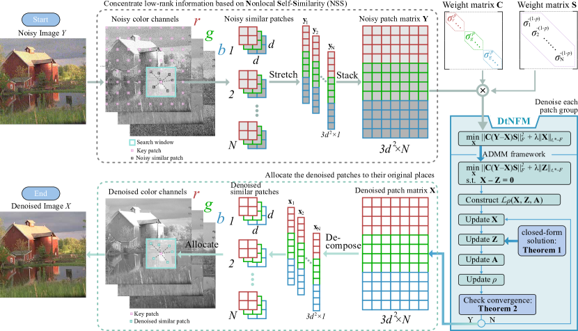
Figure 1: The schematic framework of our denoising scheme based on DtNFM model.

3 The Proposed Model for Color Image Denoising

3.1 Problem Formulation

The proposed DtNFM method is composed of two parts: 1) patch grouping via exploiting the NSS prior and 2) low-rank approximation by solving the DtNFM model. The patch grouping is to construct noisy patch matrices which will be used by the DtNFM model. And its procedure is depicted in Fig. 1. Concretely, given a noisy color image $Y\in\mathbb{R}^{H\times W\times 3}$, $P$ key patches are assigned across it. The key patches are spaced apart with an equal distance $s$, and each sizes $d\times d\times 3$ pixels. And hence the number of key patches $P=\lceil(H-p)/s\rceil\times\lceil(W-p)/s\rceil$. For each key patch, its $N$ nearest neighbors, i.e., the most similar patches, are extracted from a search window around it. Those extracted similar patches are then stretched to $N$ column vectors $\mathbf{y}_{i}\in\mathbb{R}^{3d^{2}},i\in\{1,\cdots,N\}$. The $N$ vectors are stacked horizontally to form a noisy patch matrix $\mathbf{Y}\in\mathbb{R}^{3d^{2}\times N}$. Note that the relationship between key patches and patch matrices are one-to-one. Therefore, $P$ noisy patch matrices should be constructed in total. Then, the proposed DtNFM model will operate on each of them, estimating its clean version $\mathbf{X}\in\mathbb{R}^{3d^{2}\times N}$. After that, $\mathbf{X}$ will be decomposed to $N$ vectors $\mathbf{x}_{i}\in\mathbb{R}^{3d^{2}},i\in\{1,\cdots,N\}$. For each vector, it will be reshaped back to a denoised patch and then allocated to its original place. After settling all of the $P$ denoised patch matrices, the denoised image can be obtained.

To obtain better results, the procedure above should be repeated $\theta$ iterations. And the following iterative regularization is used in order to reduce the method noise:

$$Y_{l}=X_{l-1}+\delta(Y_{0}-X_{l-1}),\quad l\in\{1,\cdots,\theta\},$$ (12)

where $\delta\in[0,1)$ is the step size of feedback, $X_{l-1}\in\mathbb{R}^{H\times W\times 3}$ is the denoised image output at the end of $(l-1)$th iteration, and $Y_{l}$ is the input image of $l$th iteration. Specifically, we set $X_{0}=Y_{0}=Y$. The complete procedure of the proposed color image denoising method is summarized in Algorithm 1.

Input: Noisy image $Y\in\mathbb{R}^{H\times W\times 3}$, noise $[\sigma_{r};\sigma_{g};\sigma_{b}]$;

Output: Denoised image $X$;

1 Initialize $X_{0}=Y_{0}=Y,\theta,s,N$;

2 for $l=1:\theta$ do

3       Iterative regularization $Y_{l}=X_{l-1}+\delta(Y_{0}-X_{l-1})$;

4       Assign $P=\lceil(H-p)/s\rceil\times\lceil(W-p)/s\rceil$ key patches in $X_{i-1}$;

5       for Each key patch do

6             Extract $N$ most similar neighbors of $j$th patch and form the patch matrix $\mathbf{Y}$;

7             Construct the weight matrices $\mathbf{C}$ and $\mathbf{S}$;

8             $\mathbf{X}=\mathrm{DtNFM\_model}(\mathbf{Y},\mathbf{C},\mathbf{S})$;

9            

10       end for

11      Aggregate all of $P$ denoised patch matrices to generate $X_{l}$;

12      

13 end for

Algorithm 1 Color image denoising via the DtNFM method.

A problem left over from Algorithm 1 is how to estimate the clean patch matrix $\mathbf{X}\in\mathbb{R}^{3d^{2}\times N}$ with high accuracy and efficiency. To this end, we propose the DtNFM model, which can be formulated as

$$\arg\min_{\bm{\mathbf{X}}}\|\mathbf{C}(\bm{\mathbf{Y}}-\bm{\mathbf{X}})\mathbf{S}\|_{F}^{2}+\lambda\|\bm{\mathbf{X}}\|_{t,*-F},$$ (13)

where $\mathbf{C}\in\mathbb{R}^{3d^{2}\times 3d^{2}}$ is the weight matrix to model the cross-channel difference of noise, $\mathbf{S}\in\mathbb{R}^{N\times N}$ is to model the spatial variation of noise, and $\|\mathbf{X}\|_{t,*-F}=\sum_{i=t+1}\sigma_{i}(\mathbf{X})-\alpha\sqrt{\sum_{i=t+1}\sigma_{i}(\mathbf{X})^{2}}$ is the truncated nuclear norm minus truncated Frobenius norm (tNF) with $t\in\mathbb{N}$ and $\alpha\geq 0$, and $\sigma_{i}(\mathbf{X})$ is the $i$th leading singular value. The proposed DtNFM model can not only model and utilize the noise exhaustively, but also estimate the underlying low-rank patch matrix with high accuracy. Moreover, it can be solved with high efficiency, which will be presented in Section 3.2. In the rest of this section, we elaborate the construction of weight matrices $\mathbf{C}$ and $\mathbf{S}$.

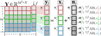
Figure 2: An illustration of the definitions of $\mathbf{y}_{j},\mathbf{x}_{j},\mathbf{x}_{j}^{(c)}$, and $\mathbf{n}_{j}$.

Given a constructed matrix $\mathbf{Y}\in\mathbb{R}^{3d^{2}\times N}$, as shown in Fig. 2, we denote the $j$th column as $\mathbf{y}_{j}=[\mathbf{y}_{j}^{(r)};\mathbf{y}_{j}^{(g)};\mathbf{y}_{j}^{(b)}]\in\mathbb{R}^{3d^{2}}$, where $\mathbf{y}_{j}^{(c)}\in\mathbb{R}^{d^{2}}$ is the observed data of channel $c\in\{r,g,b\}$. Correspondingly, define $\mathbf{x}_{j}=[\mathbf{x}_{j}^{(r)};\mathbf{x}_{j}^{(g)};\mathbf{x}_{j}^{(b)}],\mathbf{n}_{j}=[\mathbf{n}_{j}^{(r)};\mathbf{n}_{j}^{(g)};\mathbf{n}_{j}^{(b)}]\in\mathbb{R}^{3d^{2}}$ as the underlying ground truth data and the noise, respectively. Based on model (1), we have $\mathbf{y}_{j}=\mathbf{x}_{j}+\mathbf{n}_{j}$ and $\mathbf{y}_{j}^{(c)}=\mathbf{x}_{j}^{(c)}+\mathbf{n}_{j}^{(c)}$.

Given the matrix $\mathbf{Y}$, the underlying clean patch matrix $\mathbf{X}$ can be estimated through exploiting the framework of maximum a-posteriori:

$$\mathbf{X}^{*}=\arg\max_{\mathbf{X}}\mathrm{P}(\mathbf{X}|\mathbf{Y})=\arg\max_{\mathbf{X}}\frac{\mathrm{P}(\mathbf{Y}|\mathbf{X})\cdot\mathrm{P}(\mathbf{X})}{\mathrm{P}(\mathbf{Y})}=\arg\max_{\mathbf{X}}\ \ln\mathrm{P}(\mathbf{Y}|\mathbf{X})+\ln\mathrm{P}(\mathbf{X}).$$ (14)

The likelihood term $\mathrm{P}(\mathbf{Y}|\mathbf{X})$ is determined by the statistics of noise. According to [41], we assume the noise is not only independent among RGB channels, but also independent among the similar patches. In other words, we assume $(\mathbf{n}_{j}^{(c)})_{i}\stackrel{{\scriptstyle i.i.d}}{{\sim}}\mathcal{N}(0,\sigma_{cj}^{2})$ with $i\in\{1,\cdots,d^{2}\}$, where $\sigma_{cj}$ is the noise standard deviation in $j$th patch in channel $c$. And we define

$$\sigma_{cj}=\sigma_{c}^{p}\cdot\sigma_{j}^{1-p},$$ (15)

where $\sigma_{c},\sigma_{j}$ are the noise standard deviations in color channel $c$ and $j$th patch, respectively, and $p\in[0,1]$ serves as a relative weight. In practice, $\sigma_{c}$ is given or can be estimated by some noise estimation method [42]. And $\sigma_{j}$ is determined by

$$\sigma_{j}=\Big{(}\max\big{(}0,\frac{\sigma_{r}^{2}+\sigma_{g}^{2}+\sigma_{b}^{2}}{3}-\frac{1}{3d^{2}}\|\mathbf{n}_{j}\|_{2}^{2}\big{)}\Big{)}^{\frac{1}{2}},$$ (16)

where $(\sigma_{r}^{2}+\sigma_{g}^{2}+\sigma_{b}^{2})/3$ and $\frac{1}{3d^{2}}\|\mathbf{n}_{j}\|_{2}^{2}$ are the upper bound and the mean square of the noise in the $j$th patch, respectively. And the relative weight $p$ in (15) is determined by

$$p=\frac{v_{\mathbf{c}}+\epsilon}{v_{\mathbf{c}}+v_{\mathbf{s}}+2\epsilon},$$ (17)

where $v_{\mathbf{c}},v_{\mathbf{s}}\in\mathbb{R}$ are the coefficient of variation of the data vector $[\sigma_{r};\sigma_{g};\sigma_{b}]$ and $[\sigma_{1},\sigma_{2},\cdots,\sigma_{N}]$, respectively, and $\epsilon>0$ is a small real value.

After determining $\sigma_{cj}$, we can determine $\mathrm{P}(\mathbf{Y}|\mathbf{X})$ based on the Gaussian probability density function:

$$\mathrm{P}(\mathbf{Y}|\mathbf{X})=\prod_{j=1}^{N}\prod_{c\in\{r,g,b\}}\frac{1}{\sqrt{2\pi}\sigma_{cj}}\exp\Big{(}-\frac{\|\mathbf{n}_{j}^{(c)}\|_{2}^{2}}{2\sigma_{cj}^{2}}\Big{)}.$$ (18)

For the estimated patch matrix $\mathbf{X}$, the prior of possessing the minimum tNF is imposed on it. Thus we assign

$$\mathrm{P}(\mathbf{X})=\exp(-\frac{\lambda}{2}\|\mathbf{X}\|_{t,*-F})\propto\exp(-\|\mathbf{X}\|_{t,*-F}).$$ (19)

Finally, problem (14) can be deduced as

$$\mathbf{X}^{*} =\arg\max_{\mathbf{X}}\sum_{j=1}^{N}\sum_{c\in\{r,g,b\}}\big{(}-\frac{1}{2\sigma_{cj}^{2}}\|\mathbf{n}_{j}^{(c)}\|_{2}^{2}\big{)}-\frac{\lambda}{2}\|\mathbf{X}\|_{t,*-F}$$

$$=\arg\min_{\mathbf{X}}\sum_{j=1}^{N}{\sigma_{j}^{-2(1-p)}}\sum_{c\in\{r,g,b\}}{\sigma_{c}^{-2p}}\|\mathbf{y}_{j}^{(c)}-\mathbf{x}_{j}^{(c)}\|_{2}^{2}+\lambda\|\mathbf{X}\|_{t,*-F}$$

$$=\arg\min_{\mathbf{X}}\sum_{j=1}^{N}{\sigma_{j}^{-2(1-p)}}\|\mathbf{C}(\mathbf{y}_{j}-\mathbf{x}_{j})\|_{2}^{2}+\lambda\|\mathbf{X}\|_{t,*-F}$$

$$=\arg\min_{\mathbf{X}}\|\mathbf{C}(\mathbf{Y}-\mathbf{X})\mathbf{S}\|_{F}^{2}+\lambda\|\mathbf{X}\|_{t,*-F},$$ (20)

where $\mathbf{C}=\mathrm{Diag}([\sigma_{r}^{-p}\mathbf{1};\sigma_{g}^{-p}\mathbf{1};\sigma_{b}^{-p}\mathbf{1}])\in\mathbb{R}^{3d^{2}\times 3d^{2}}$, and $\mathbf{S}=\mathrm{Diag}([\sigma_{1}^{-(1-p)},\cdots,\sigma_{N}^{-(1-p)}])\in\mathbb{R}^{N\times N}$. Intuitively, as $\sigma_{c}$ becomes larger, the data in color channel $c$ will make less contribution to the estimation of $\mathbf{X}$. In the same manner, a larger $\sigma_{j}$ will reduce the contribution of $j$th noisy patch when estimating $\mathbf{X}$.

3.2 Optimization

To solve the proposed DtNFM model, an efficient and effective algorithm is proposed via exploiting the framework of the ADMM. According to section 2.2, the original problem (13) can be rewritten as

$$\arg\min_{\mathbf{X},\mathbf{Z}}\|\mathbf{C}(\bm{\mathbf{Y}}-\bm{\mathbf{X}})\mathbf{S}\|_{F}^{2}+\lambda\|\bm{\mathbf{Z}}\|_{t,*-F},$$

$$\ \mathrm{s.t.}\ \ \mathbf{X}-\mathbf{Z}=\mathbf{0},$$ (21)

where $\mathbf{Z},\mathbf{0}\in\mathbb{R}^{3d^{2}\times N}$ are the auxiliary variable and a matrix of zeros, respectively. The augmented Lagrangian of problem (21) is

$$\mathcal{L}_{\rho}(\mathbf{X},\mathbf{Z},\mathbf{A})=\|\mathbf{C}(\bm{\mathbf{Y}}-\bm{\mathbf{X}})\mathbf{S}\|_{F}^{2}+\lambda\|\bm{\mathbf{Z}}\|_{t,*-F}+\langle\mathbf{A},\mathbf{X}-\mathbf{Z}\rangle+\frac{\rho}{2}\|\mathbf{X}-\mathbf{Z}\|_{F}^{2},$$ (22)

where $\mathbf{A}\in\mathbb{R}^{3d^{2}\times N}$ is the Lagrangian multiplier, and $\rho>0$ is the penalty parameter. The proposed algorithm solves the following subproblems alternatively until convergence.

$$\mathbf{X}_{k+1}=\arg\min_{\mathbf{X}}\mathcal{L}_{\rho_{k}}(\mathbf{X},\mathbf{Z}_{k},\mathbf{A}_{k}),$$ (23)

$$\mathbf{Z}_{k+1}=\arg\min_{\mathbf{Z}}\mathcal{L}_{\rho_{k}}(\mathbf{X}_{k+1},\mathbf{Z},\mathbf{A}_{k}),$$ (24)

$$\mathbf{A}_{k+1}=\mathbf{A}_{k}+\rho_{k}(\mathbf{X}_{k+1}-\mathbf{Z}_{k+1}),$$ (25)

$$\ \rho_{k+1}=\mu\!\cdot\!\rho_{k},$$ (26)

where $k\in\mathbb{N}$ is the iteration number and $\mu>1$ is a scaler. To drive the algorithm to convergence, equation (26) is used to make the $\rho_{k}\rightarrow+\infty$ as $k\rightarrow\infty$. In the rest of this section, we detail the subproblems (23) and (24).

For subproblem (23), we have

$$\mathbf{X}_{k+1} =\arg\min_{\mathbf{X}}\|\mathbf{C}(\mathbf{Y}-\mathbf{X})\mathbf{S}\|_{F}^{2}+\lambda\|\mathbf{Z}_{k}\|_{t,*-F}+\langle\mathbf{A}_{k},\mathbf{X}-\mathbf{Z}_{k}\rangle+\frac{\rho_{k}}{2}\|\mathbf{X}-\mathbf{Z}_{k}\|_{F}^{2}$$

$$=\arg\min_{\mathbf{X}}\|\mathbf{C}(\mathbf{Y}-\mathbf{X})\mathbf{S}\|_{F}^{2}\!+\!\frac{\rho_{k}}{2}\|\mathbf{X}\!-\!\mathbf{Z}_{k}\!+\!\frac{1}{\rho_{k}}\mathbf{A}_{k}\|_{F}^{2}.$$ (27)

This is a standard least squares problem, which has a closed-form solution:

$$\mathbf{X}_{k+1}=(2\mathbf{C}^{2}\mathbf{Y}\mathbf{S}^{2}+\rho_{k}\mathbf{Z}_{k}-\mathbf{A}_{k})\oslash(2\mathbf{C}^{2}\mathbf{1}\mathbf{S}^{2}+\rho_{k}\mathbf{1}),$$ (28)

where $\mathbf{1}\in\mathbb{R}^{3d^{2}\times N}$ is a matrix of ones. The solution in (28) can be equivalently rewritten in an entrywise manner:

$$(\mathbf{X}_{k+1})_{ij}=\frac{2\mathbf{C}_{ii}^{2}\mathbf{Y}_{ij}\mathbf{S}_{jj}^{2}+\rho_{k}(\mathbf{Z}_{k})_{ij}-(\mathbf{A}_{k})_{ij}}{2\mathbf{C}_{ii}^{2}\mathbf{S}_{jj}^{2}+\rho_{k}},\quad\forall i\in\{1,\cdots,3d^{2}\},j\in\{1,\cdots,N\}.$$ (29)

Subproblem (24) can be equivalently rewritten as

$$\mathbf{Z}_{k+1}\!=\!\arg\min_{\mathbf{Z}}\frac{1}{2}\|\mathbf{Z}-(\mathbf{X}_{k+1}+\frac{1}{\rho_{k}}\mathbf{A}_{k})\|_{F}^{2}\!+\!\frac{\lambda}{\rho_{k}}\|\mathbf{Z}\|_{t,*-F}.$$ (30)

Problem (30) is nonconvex, which is rather difficult to solve by traditional optimization techniques. To address this issue, we propose the following theorem to show that the global optimum of problem (30) can be obtained in closed-form.

Theorem 1.

Assume that $\tau>0$ and $\mathbf{B}\in\mathbb{R}^{m\times n}$ admits SVD as $\mathbf{U}_{\mathbf{B}}\mathrm{Diag}(\bm{\sigma}(\mathbf{B}))\mathbf{V}_{\mathbf{B}}^{\top}$, without loss of generality, let $m\geq n$. Then, the closed-form solution to

$$\arg\min_{\mathbf{Z}}\frac{1}{2}\|\mathbf{Z}-\mathbf{B}\|_{F}^{2}+\tau\|\mathbf{Z}\|_{t,*-F},$$ (31)

is given by

$$\mathbf{Z}^{*}=\mathbf{U}_{\mathbf{B}}\mathrm{Diag}(\varrho^{*})\mathbf{V}_{\mathbf{B}}^{\top},$$ (32)

where

$$\varrho^{*}_{i}\!=\!\left\{\begin{array}[]{ll}\!\!\sigma_{i}(\mathbf{B}),&\!\!\!\!\!\mathrm{if}\ \ 0\leq i<t+1,\\ \!\!\!\bigl{(}1+\frac{\tau}{\|\mathcal{S}_{\tau}(\mathbf{r})\|_{2}}\bigr{)}\mathcal{S}_{\tau}(\sigma_{i}(\mathbf{B})),&\!\!\!\!\!\mathrm{if}\ \ t+1\leq i\leq n,\end{array}\right.$$ (33)

where $\mathbf{r}=[0,\cdots,0,\sigma_{t+1}(\mathbf{B}),\cdots,\sigma_{n}(\mathbf{B})]^{\top}$ and $\mathcal{S}_{\tau}(\mathbf{r})_{i}=\max(\mathbf{r}_{i}-\tau,0)$ be the soft shrinkage [23].

Proof 1.

Consider $\mathbf{Z}$ admits SVD as $\mathbf{U}_{\mathbf{Z}}\mathbf{\Sigma}_{\mathbf{Z}}\mathbf{V}_{\mathbf{Z}}^{\top}$. The first term of problem (31) can be rewritten as

$$\frac{1}{2}\|\mathbf{Z}-\mathbf{B}\|_{F}^{2}=\frac{1}{2}\left(\|\mathbf{Z}\|_{F}^{2}-2\langle\mathbf{Z},\mathbf{B}\rangle+\|\mathbf{B}\|_{F}^{2}\right).$$ (34)

According to Von Neumann’s trace inequality, we have

$$\langle\mathbf{Z},\mathbf{B}\rangle= \mathrm{tr}(\mathbf{Z}^{\top}\mathbf{B})=\mathrm{tr}(\mathbf{V}_{\mathbf{Z}}\mathbf{\Sigma}_{\mathbf{Z}}\mathbf{U}_{\mathbf{Z}}^{\top}\mathbf{B})=\mathrm{tr}(\mathbf{\Sigma}_{\mathbf{Z}}\mathbf{U}_{\mathbf{Z}}^{\top}\mathbf{B}\mathbf{V}_{\mathbf{Z}})$$

$$\leq \sum_{i=1}^{n}\sigma_{i}(\mathbf{Z})\!\cdot\!\sigma_{i}(\mathbf{B})\!\cdot\!\sigma_{i}(\mathbf{U}_{\mathbf{Z}}^{\top}\mathbf{V}_{\mathbf{Z}})=\sum_{i=1}^{n}\sigma_{i}(\mathbf{Z})\!\cdot\!\sigma_{i}(\mathbf{B}).$$ (35)

The equality of (35) occurs if and only if

$$\mathbf{U}_{\mathbf{Z}}=\mathbf{U}_{\mathbf{B}},\mathbf{V}_{\mathbf{Z}}=\mathbf{V}_{\mathbf{B}}.$$ (36)

Therefore, problem (31) can be rewritten as follows:

$$\arg\min_{\mathbf{Z}}\frac{1}{2}\|\mathbf{Z}-\mathbf{B}\|_{F}^{2}+\tau\|\mathbf{Z}\|_{t,*-F}$$

$$= \arg\min_{\mathbf{Z}}\frac{1}{2}\|\mathbf{Z}\|_{F}^{2}-\sum_{i=1}^{n}\sigma_{i}(\mathbf{Z})\sigma_{i}(\mathbf{B})+\frac{1}{2}\|\mathbf{B}\|_{F}^{2}+\tau\biggl{(}\sum_{i=t+1}^{n}\sigma_{i}(\mathbf{Z})-\bigl{(}\sum_{i=t+1}^{n}\sigma_{i}(\mathbf{Z})^{2}\bigr{)}^{\frac{1}{2}}\biggr{)}$$

$$= \arg\min_{\mathbf{Z}}\sum_{i=1}^{n}\!\left(\frac{1}{2}\sigma_{i}(\mathbf{Z})^{2}-\sigma_{i}(\mathbf{Z})\sigma_{i}(\mathbf{B})\!\right)\!+\!\sum_{i=t+1}^{n}\!\biggl{(}\frac{1}{2}\sigma_{i}(\mathbf{Z})^{2}-\sigma_{i}(\mathbf{Z})\sigma_{i}(\mathbf{B})+\tau\sigma_{i}(\mathbf{Z})\!\biggr{)}\!-\tau\!\biggl{(}\sum_{i=t+1}^{n}\sigma_{i}(\mathbf{Z})^{2}\!\biggr{)}^{\frac{1}{2}}.$$ (37)

Therefore, the original problem (31) has been equivalently transformed into the combination of independent quadratic equations for each $\sigma_{i}(\mathbf{Z})$. Let $F(\bm{\sigma}(\mathbf{Z}))$ denote the objective function of (37). The minimum of $F$, denoted as $\varrho^{*}_{i}$, is given by

$$\frac{\partial F}{\partial{\sigma_{i}}(\mathbf{Z})}=0.$$ (38)

When $0\leq i<t+1$, it is trivial to obtain

$$\varrho^{*}_{i}=\sigma_{i}(\mathbf{B}).$$ (39)

When $t+1\leq i\leq n$, equation (38) is expressed as

$$\Bigl{(}1-\frac{\tau}{\|\bm{\sigma}(\mathbf{Z})\|_{2}}\Bigr{)}\bm{\sigma}(\mathbf{Z})=\bm{\sigma}(\mathbf{B})-\tau.$$ (40)

Let $\mathbf{r}=[0,\ldots,0,\sigma_{t+1}(\mathbf{B}),\ldots,\sigma_{T}(\mathbf{B})]^{\top}\in\mathbb{R}^{n}$ and $\mathcal{S}_{\tau}(\mathbf{r})_{i}=\max(\mathbf{r}_{i}-\tau,0)$, the solution of (40) is

$$\varrho^{*}_{i}=\Bigl{(}1+\frac{\tau}{\|\mathcal{S}_{\tau}(\mathbf{r})\|_{2}}\Bigr{)}\!\cdot\!\mathcal{S}_{\tau}(\sigma_{i}(\mathbf{B})).$$ (41)

Combining (39) and (40), the minimum of $F$ is obtained at

$$\varrho^{*}_{i}\!=\!\left\{\begin{array}[]{ll}\!\!\sigma_{i}(\mathbf{B}),&\!\!\!\!\!\mathrm{if}\ \ 0\leq i<t+1,\\ \!\!\!\bigl{(}1+\frac{\tau}{\|\mathcal{S}_{\tau}(\mathbf{r})\|_{2}}\bigr{)}\mathcal{S}_{\tau}(\sigma_{i}(\mathbf{B})),&\!\!\!\!\!\mathrm{if}\ \ t+1\leq i<n+1.\end{array}\right.$$ (42)

Therefore, the optimal solution of problem (13) is

$$\mathbf{Z}^{*}=\mathbf{U}_{\mathbf{B}}\mathrm{Diag}(\varrho^{*})\mathbf{V}_{\mathbf{B}}^{\top}.$$ (43)

∎

According to Theorem 1, the global optimum of subproblem (24) is given by (32) and (33), where $\mathbf{B}=\mathbf{X}_{k+1}+\rho_{k}^{-1}\mathbf{A}_{k}$ and $\tau=\lambda/\rho_{k}$. Up to now, the global optima of both subproblem (23) and (24) have been obtained in closed-form.

The algorithm would be terminated when the iteration number exceeds a threshold $K$ or the following stopping criteria hold simultaneously:

$$(a)\|\mathbf{X}_{k+1}-\mathbf{Z}_{k+1}\|_{F}\leq\epsilon,(b)\|\mathbf{X}_{k+1}-\mathbf{X}_{k}\|_{F}\leq\epsilon,(c)\|\mathbf{Z}_{k+1}-\mathbf{Z}_{k}\|_{F}\leq\epsilon,$$ (44)

where $\epsilon>0$ is a small tolerance. The stopping criterion in (44) is according to the convergence result given by Theorem 2. Finally, the complete algorithm for solving problem (13) is summarized in Algorithm 2.

Input: Noisy matrix $\mathbf{Y}$, weight matrix $\mathbf{C},\mathbf{S}$;

Output: Denoised matrix $\mathbf{X}$;

1 Initialize $\mathbf{X}_{0}=\mathbf{Z}_{0}=\mathbf{A}_{0}=\mathbf{0},\rho_{0},t,\lambda,\mu,\varepsilon,k=0,K$;

2 while Stopping criterion is not satisfied do

3       $\mathbf{X}_{k+1}\leftarrow$ the right side of (28);

4       $\mathbf{Z}_{k+1}\leftarrow$ the right side of (30);

5       $\mathbf{A}_{k+1}\leftarrow\mathbf{A}_{k}+\rho_{k}(\mathbf{X}_{k+1}-\mathbf{Z}_{k+1})$;

6       $\rho_{k+1}\;\leftarrow\mu\cdot\rho_{k}$;

7       Check the stopping criterion: $((k\leftarrow k+1)>K)||(\|\mathbf{X}_{k+1}-\mathbf{Z}_{k+1}\|_{F}\leq\varepsilon)\&\&$ $(\|\mathbf{Z}_{k+1}-\mathbf{Z}_{k}\|_{F}\leq\varepsilon)\&\&(\|\mathbf{X}_{k+1}-\mathbf{X}_{k}\|_{F}\leq\varepsilon)$;

8      

9 end while

Algorithm 2 Solving DtNFM model via ADMM.

3.3 Convergence and Complexity Analysis

In this section, we propose the following theorem to give a weak convergence result for Algorithm 2.

Theorem 2.

The sequences $\{\mathbf{X}_{k}\}$ and $\{\mathbf{Z}_{k}\}$ generated by Algorithm 2 satisfy

$$a)\lim_{k\rightarrow\infty}\|\mathbf{X}_{k+1}-\mathbf{Z}_{k+1}\|_{F}\!=0,\quad b)\!\lim_{k\rightarrow\infty}\|\mathbf{X}_{k+1}-\mathbf{X}_{k}\|_{F}\!=0,\quad c)\lim_{k\rightarrow\infty}\|\mathbf{Z}_{k+1}-\mathbf{Z}_{k}\|_{F}=0.$$ (45)

Proof 2.

The sequence of Lagrangian multiplier $\{\mathbf{A}_{k}\}$ is upper bounded since

$$\|\mathbf{A}_{k+1}\|_{F}^{2} =\|\mathbf{A}_{k}+\rho_{k}(\mathbf{X}_{k+1}-\mathbf{Z}_{k})\|_{F}^{2}$$

$$=\rho^{2}_{k}\|(\rho_{k}^{-1}\mathbf{A}_{k}+\mathbf{X}_{k+1})-\mathbf{Z}_{k+1}\|_{F}^{2}$$

$$=\rho^{2}_{k}\|\mathbf{U}_{\mathbf{B}}\mathbf{\Sigma}_{\mathbf{B}}\mathbf{V}_{\mathbf{B}}^{\top}-\mathbf{U}_{\mathbf{B}}\mathrm{Diag}(\varrho^{*})\mathbf{V}_{\mathbf{B}}^{\top}\|_{F}^{2}$$

$$=\rho^{2}_{k}\sum_{i=t+1}^{N}(\sigma_{i}(\mathbf{B})-\varrho_{i}^{*})^{2},$$ (46)

where $\mathbf{B}=\mathbf{X}_{k+1}+\rho_{k}^{-1}\mathbf{A}_{k}\in\mathbb{R}^{3d^{2}\times N}$, without loss of generality, assume $3d^{2}\geq N$. If $\sigma_{i}(\mathbf{B})>\lambda/\rho_{k}$, $\varrho_{i}^{*}=(1+\frac{\lambda/\rho_{k}}{\|\mathcal{S}_{\lambda/\rho_{k}}(\mathbf{r})\|_{2}})\!\cdot\!(\sigma_{i}(\mathbf{B})-\lambda/\rho_{k})$. Let $\phi=1+\frac{\lambda/\rho_{k}}{\|\mathcal{S}_{\lambda/\rho_{k}}(\mathbf{r})\|_{2}}$. We have $\sigma_{i}(\mathbf{B})-\varrho_{i}^{*}=(1-\phi)\sigma_{i}(\mathbf{B})+\phi\lambda/\rho_{k}<\lambda/\rho_{k}$. If $\sigma_{i}(\mathbf{B})\leq\lambda/\rho_{k}$, $\varrho_{i}^{*}=0$. We have $\sigma_{i}(\mathbf{B})-\varrho_{i}^{*}=\sigma_{i}(\mathbf{B})\leq\lambda/\rho_{k}$. Overall, we have $\sigma_{i}(\mathbf{B})-\varrho_{i}^{*}\leq\lambda/\rho_{k}$. Then we can deduce

$$\|\mathbf{A}_{k+1}\|_{F}^{2} \leq\rho_{k}^{2}{\sum_{i=t+1}^{N}}(\lambda/\rho_{k})^{2}=\lambda^{2}(n-t).$$ (47)

Since $\{\mathbf{A}_{k}\}$ is upper bounded, $\{\mathbf{A}_{k+1}-\mathbf{A}_{k}\}$ is upper bounded, i.e., $\exists M>0,\forall k\geq 0,\|\mathbf{A}_{k+1}-\mathbf{A}_{k}\|_{F}\leq M$. According to the squeeze theorem, we have

$$0\leq\lim_{k\rightarrow\infty}\|\mathbf{X}_{k+1}-\mathbf{Z}_{k+1}\|_{F}=\lim_{k\rightarrow\infty}\rho_{k}^{-1}\|\mathbf{A}_{k+1}-\mathbf{A}_{k}\|_{F}\leq\lim_{k\rightarrow\infty}\frac{M}{\rho_{k}}=0.$$ (48)

Therefore, (a) is proved.

The objective function in (21) can be transformed as follows

$$\|\mathbf{C}(\mathbf{Y}-\mathbf{X})\mathbf{S}\|_{F}^{2}+\lambda\|\mathbf{Z}\|_{t,*-F}$$

$$= \mathcal{L}_{\rho_{k-1}}(\mathbf{X}_{k},\mathbf{Z}_{k},\mathbf{A}_{k-1})-\langle\mathbf{A}_{k-1},\mathbf{X}_{k}-\mathbf{Z}_{k}\rangle-\rho_{k-1}/2\|\mathbf{X}_{k}-\mathbf{Z}_{k}\|_{F}^{2}$$

$$= \mathcal{L}_{\rho_{k-1}}(\mathbf{X}_{k},\mathbf{Z}_{k},\mathbf{A}_{k-1})-\langle\mathbf{A}_{k-1},(\mathbf{A}_{k}-\mathbf{A}_{k-1})/\rho_{k}\rangle-\rho_{k-1}/2\|(\mathbf{A}_{k}-\mathbf{A}_{k-1})/\rho_{k}\|_{F}^{2}$$

$$= \mathcal{L}_{\rho_{k-1}}(\mathbf{X}_{k},\mathbf{Z}_{k},\mathbf{A}_{k-1})+(2\rho_{k})^{-1}(\|\mathbf{A}_{k-1}-\mathbf{A}_{k}\|_{F}^{2}),$$ (49)

where $k\in\mathbb{N}_{+}$. The augmented Lagrangian term of (49) satisfies

$$\mathcal{L}_{\rho_{k-1}}(\mathbf{X}_{k},\mathbf{Z}_{k},\mathbf{A}_{k-1})\leq\mathcal{L}_{\rho_{k-1}}(\mathbf{X}_{k-1},\mathbf{Z}_{k-1},\mathbf{A}_{k-1}),$$ (50)

since the global optimum of $\mathbf{X}$ and $\mathbf{Z}$ can be got from step 3 and 4 in Algorithm 2. Then we have

$$\mathcal{L}_{\rho_{k}}(\mathbf{X}_{k},\mathbf{Z}_{k},\mathbf{A}_{k})$$

$$= \mathcal{L}_{\rho_{k-1}}(\mathbf{X}_{k},\mathbf{Z}_{k},\mathbf{A}_{k-1})+\langle\mathbf{A}_{k}-\mathbf{A}_{k-1},\mathbf{X}_{k}-\mathbf{Z}_{k}\rangle+(\rho_{k}-\rho_{k-1})/2\|\mathbf{X}_{k}-\mathbf{Z}_{k}\|_{F}^{2}$$

$$= \mathcal{L}_{\rho_{k-1}}(\mathbf{X}_{k},\mathbf{Z}_{k},\mathbf{A}_{k-1})+\langle\mathbf{A}_{k}-\mathbf{A}_{k-1},\frac{\mathbf{A}_{k}-\mathbf{A}_{k-1}}{\rho_{k}}\rangle+(\rho_{k}-\rho_{k-1})/(2\rho_{k-1}^{2})\|\mathbf{A}_{k}-\mathbf{A}_{k-1}\|_{F}^{2}$$

$$\leq \mathcal{L}_{\rho_{k-1}}(\mathbf{X}_{k},\mathbf{Z}_{k},\mathbf{A}_{k-1})+\frac{\rho_{k}+\rho_{k-1}}{2\rho_{k-1}^{2}}\!\cdot\!M^{2}$$

$$\leq \mathcal{L}_{\rho_{0}}(\mathbf{X}_{1},\mathbf{Z}_{1},\mathbf{A}_{0})+M^{2}{\textstyle\sum_{k=1}^{\infty}}\frac{\rho_{k}+\rho_{k-1}}{2\rho_{k-1}^{2}}=\mathcal{L}_{\rho_{0}}(\mathbf{X}_{1},\mathbf{Z}_{1},\mathbf{A}_{0})+M^{2}{\textstyle\sum_{k=1}^{\infty}}\frac{\mu+1}{2\mu^{k-1}\rho_{0}}$$

$$\leq \mathcal{L}_{\rho_{0}}(\mathbf{X}_{1},\mathbf{Z}_{1},\mathbf{A}_{0})+\frac{M^{2}}{\rho_{0}}{\textstyle\sum_{k=1}^{\infty}}\frac{1}{\mu^{k-2}},$$ (51)

where the last inequality holds as $\mu+1<2\mu$. Since $\sum_{k=0}^{\infty}\frac{1}{\mu^{k-2}}<\infty$, $\{\mathcal{L}_{\rho_{k-1}}(\mathbf{X}_{k},\mathbf{Z}_{k},\mathbf{A}_{k-1})\}$ is upper bounded. Therefore, the objective function in (21) is upper bounded. And both $\|\mathbf{C}(\mathbf{Y}-\mathbf{X})\|_{F}^{2}$ and $\lambda\|\mathbf{Z}\|_{t,*-F}$ are upper bounded since both them are positive. Then we can prove (b) and (c).

$$\lim_{k\rightarrow\infty}\|\mathbf{X}_{k+1}-\mathbf{X}_{k}\|_{F}$$

$$= \lim_{k\rightarrow\infty}\|(2\mathbf{C}^{2}\mathbf{Y}\mathbf{S}^{2}+\rho_{k}\mathbf{Z}_{k}-\mathbf{A}_{k})\oslash(2\mathbf{C}^{2}\mathbf{1}\mathbf{S}^{2}+\rho_{k}\mathbf{1})-\frac{1}{\rho_{k-1}}(\mathbf{A}_{k}-\mathbf{A}_{k-1})-\mathbf{Z}_{k}\|_{F}$$

$$= \lim_{k\rightarrow\infty}\|(2\mathbf{C}^{2}\mathbf{Y}\mathbf{S}^{2}-2\mathbf{C}^{2}\mathbf{Z}_{k}\mathbf{S}^{2}-\mathbf{A}_{k})\oslash(2\mathbf{C}^{2}\mathbf{1}\mathbf{S}^{2}+\rho_{k}\mathbf{1})-\frac{1}{\rho_{k-1}}(\mathbf{A}_{k}-\mathbf{A}_{k-1})\|_{F}$$

$$= \lim_{k\rightarrow\infty}\|(2\mathbf{C}^{2}\mathbf{Y}\mathbf{S}^{2}-2\mathbf{C}^{2}(\mathbf{X}_{k}+\frac{1}{\rho_{k-1}}(\mathbf{A}_{k-1}-\mathbf{A}_{k}))\mathbf{S}^{2}-\mathbf{A}_{k})\oslash(2\mathbf{C}^{2}\mathbf{1}\mathbf{S}^{2}+\rho_{k}\mathbf{1})-\frac{1}{\rho_{k-1}}(\mathbf{A}_{k}-\mathbf{A}_{k-1})\|_{F}$$

$$= \lim_{k\rightarrow\infty}\|(2\mathbf{C}^{2}(\mathbf{Y}-\mathbf{X}_{k})\mathbf{S}^{2}-\frac{2}{\rho_{k-1}}\mathbf{C}^{2}\mathbf{A}_{k-1}\mathbf{S}^{2}+(\frac{2}{\rho_{k-1}}\mathbf{C}^{2}\mathbf{1}\mathbf{S}^{2}-\mathbf{1})\odot\mathbf{A}_{k})$$

$$\quad\oslash(2\mathbf{C}^{2}\mathbf{1}\mathbf{S}^{2}+\rho_{k}\mathbf{1})-\frac{1}{\rho_{k-1}}(\mathbf{A}_{k}-\mathbf{A}_{k-1})\|_{F}$$

$$\leq \lim_{k\rightarrow\infty}\|2\mathbf{C}^{2}(\mathbf{Y}-\mathbf{X}_{k})\mathbf{S}^{2}\oslash(2\mathbf{C}^{2}\mathbf{1}\mathbf{S}^{2}+\rho_{k}\mathbf{1})\|_{F}+\|\frac{2}{\rho_{k-1}}\mathbf{C}^{2}\mathbf{A}_{k-1}\mathbf{S}^{2}\oslash(2\mathbf{C}^{2}\mathbf{1}\mathbf{S}^{2}+\rho_{k}\mathbf{1})\|_{F}$$

$$\quad+\|(\frac{2}{\rho_{k-1}}\mathbf{C}^{2}\mathbf{1}\mathbf{S}^{2}-\mathbf{1})\odot\mathbf{A}_{k}\oslash(2\mathbf{C}^{2}\mathbf{1}\mathbf{S}^{2}+\rho_{k}\mathbf{1})\|_{F}=0.$$ (52)

$$\lim_{k\rightarrow\infty}\|\mathbf{Z}_{k+1}-\mathbf{Z}_{k}\|_{F}$$

$$= \lim_{k\rightarrow\infty}\|\frac{1}{\rho_{k}}(\mathbf{A}_{k}-\mathbf{A}_{k+1})+\mathbf{X}_{k+1}-\mathbf{Z}_{k}\|_{F}$$

$$= \lim_{k\rightarrow\infty}\|(\mathbf{X}_{k}+\frac{1}{\rho_{k-1}}\mathbf{A}_{k-1}-\mathbf{Z}_{k})+(\mathbf{X}_{k+1}-\mathbf{X}_{k})-\frac{1}{\rho_{k-1}}\mathbf{A}_{k-1}+\frac{1}{\rho_{k}}(\mathbf{A}_{k}-\mathbf{A}_{k+1})\|_{F}$$

$$\leq \lim_{k\rightarrow\infty}\frac{1}{\rho_{k-1}}\|\mathbf{A}_{k}\|_{F}+\|\mathbf{X}_{k+1}-\mathbf{X}_{k}\|_{F}+\frac{1}{\rho_{k-1}}\|\mathbf{A}_{k-1}\|_{F}-\frac{1}{\rho_{k}}\|\mathbf{A}_{k}+\mathbf{A}_{k+1}\|_{F}=0.$$ (53)

∎

Theorem 2 ensures that $\{\mathbf{X}_{k}\}$ and $\{\mathbf{Z}_{k}\}$ converge to a single critical point, i.e., $\lim_{k\rightarrow\infty}\mathbf{X}_{k}=\lim_{k\rightarrow\infty}\mathbf{Z}_{k}=\mathbf{X}^{*}$. According to Theorem 2, rational stopping criteria are established in (44).

The time complexity of Algorithm 2 is discussed in brief. In step 3, updating $\mathbf{X}\in\mathbb{R}^{3d^{2}\times N}$ takes $\mathcal{O}(d^{4}N)$ time. In step 4, the complexity is $\mathcal{O}(d^{2}N^{2}+d^{4}N)$ since the SVD of $\mathbf{Z}\in\mathbb{R}^{3d^{2}\times N}$ costs $\mathcal{O}(d^{2}N^{2})$ time. The complexity of step 5 is $\mathcal{O}(d^{2}N)$. Therefore, the complexity of Algorithm 2 is $\mathcal{O}((d^{4}N+d^{2}N^{2})K)$. In Algorithm 1, step 5 costs $\mathcal{O}(S^{2}\log S)$ time, where $S\in\mathbb{N}_{+}$ is the side length of the search window. In step 6, constructing $\mathbf{C}\in\mathbb{R}^{3d^{2}\times 3d^{2}}$ and $\mathbf{S}\in\mathbb{R}^{N\times N}$ costs $\mathcal{O}(d^{4}+N^{2})$ time. The predominant cost lies in step 7, which is actually the Algorithm 2. In summary, the complexity of Algorithm 1 is $\mathcal{O}((d^{4}N+d^{2}N^{2})KP\theta)$.

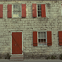
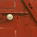
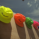
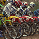
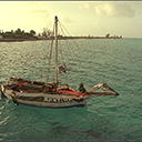
(a)

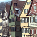
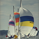
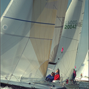
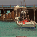
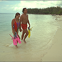
(b)

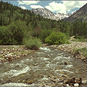
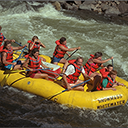
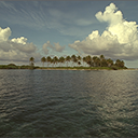
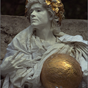
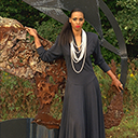
(c)

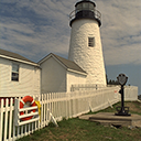
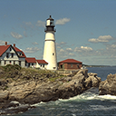
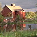
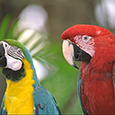
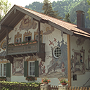
(d)

Figure 3: Test images in Kodak24 data set (enumerated from left-to-right and top-to-bottom).

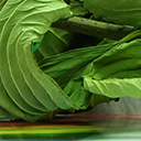
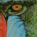
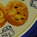
(a)

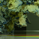
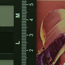
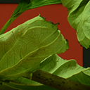
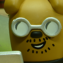
(b)

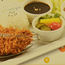
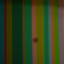
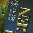
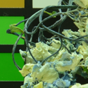
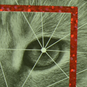
(c)

Figure 4: The noise-free images in CC15 data set (#1 to #15, enumerated from left-to-right and top-to-bottom).

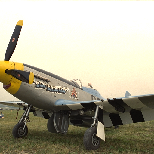
(a)

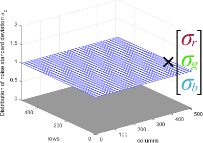
(b)

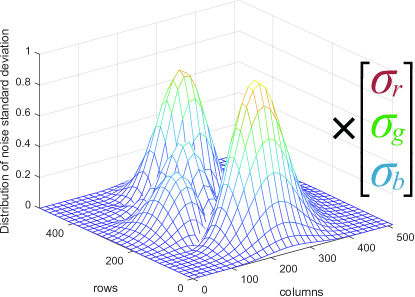
(c)

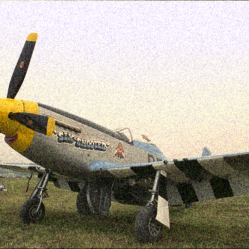
(d)

(e)

Figure 5: Illustrations of the distribution of noise standard deviation and the corresponding noisy images. (a) the ground truth of image “kodim20.png”. (b) The surface of the noise standard deviation. (c) The surface of noise standard deviation returned by MATLAB code “abs(peaks(512))”. A point $(x,y,z)$ means that for the pixel at $x$th row and $y$th column, the noise standard deviations on it are $z\times[\sigma_{r};\sigma_{g};\sigma_{b}]$, respectively, where $z\in[0,1]$. Specifically, $z\equiv 1$ in subfigure (b). (d) The noisy image generated by the noise in subfigure (b) with $[\sigma_{r};\sigma_{g};\sigma_{b}]=[20;35;5]$. (e) The noisy image generated by the noise in subfigure (c) with $[\sigma_{r};\sigma_{g};\sigma_{b}]=[30;35;40]$.

4 Experimental Results and Analysis

To test the performance of the proposed DtNFM method, three kinds of experiments are conducted. In the first experiment, we synthesize the noise which has only cross-channel difference. In the second experiment, the noise is synthesized to possess both cross-channel difference and spatial variation. Those two experiments are implemented on the Kodak24 data set, which includes 24 noise-free color images, as shown in Fig. 3. In the third experiment, we denoise the real-world images in the CC15 data set [43], which includes 15 noisy color images and their corresponding noise-free versions, as shown in Fig. 4. Seven state-of-the-art methods are compared, including (a) CBM3D [36], (b) LRQA [28], (c) DnCNN [12], (d) FFDNet [13], (e) MCWNNM [37], (f) MCWSNM [39], and (g) NNFNM [11]. The parameters of compared methods are either tuned to the optimum or kept the same as the original codes.

Table 1:
PSNR(dB) and SSIM results for all competing methods under $[\sigma_{r};\sigma_{g};\sigma_{b}]=[20;35;5]$.

	​​CBM3D	​​LRQA	​​MCWNNM	​​MCWSNM	​​FFDNet	​​DnCNN	​​NNFNM	​​DtNFM
#	​​PSNR SSIM	​​PSNR SSIM	​​PSNR SSIM	​​PSNR SSIM	​​PSNR SSIM	​​PSNR SSIM	​​PSNR SSIM	​​PSNR SSIM
1	​​28.66 0.8267	​​27.48 0.7942	​​31.19 0.9058	​​31.11 0.9030	​​29.90 0.8707	​​29.94 0.8728	​​31.47 0.9088	​​31.58 0.9118
2	​​31.53 0.7683	​​31.04 0.7552	​​34.02 0.8662	​​34.02 0.8682	​​33.02 0.8412	​​33.00 0.8407	​​34.07 0.8645	​​34.12 0.8704
3	​​33.16 0.8454	​​32.28 0.8313	​​35.84 0.9144	​​35.96 0.8682	​​35.06 0.9165	​​34.97 0.9151	​​35.98 0.9117	​​36.30 0.9197
4	​​31.71 0.8017	​​31.05 0.7861	​​34.59 0.9233	​​34.60 0.8922	​​33.12 0.8647	​​33.09 0.8640	​​34.68 0.8889	​​34.78 0.8950
5	​​29.17 0.8657	​​27.86 0.8362	​​31.24 0.9233	​​31.23 0.9227	​​30.63 0.9030	​​30.68 0.9026	​​31.59 0.9265	​​31.68 0.9308
6	​​29.98 0.8251	​​28.68 0.7897	​​32.51 0.9016	​​32.45 0.9016	​​31.21 0.8779	​​31.19 0.8780	​​32.71 0.9038	​​32.75 0.9083
7	​​32.30 0.8749	​​31.65 0.8713	​​34.89 0.9332	​​35.02 0.9401	​​34.53 0.9399	​​34.49 0.9392	​​35.05 0.9307	​​35.13 0.9348
8	​​29.27 0.8766	​​27.94 0.8583	​​31.26 0.9277	​​31.28 0.9269	​​30.33 0.9029	​​30.45 0.9041	​​31.45 0.9289	​​31.66 0.9324
9	​​32.69 0.8445	​​31.75 0.8345	​​35.16 0.9101	​​35.27 0.9164	​​34.73 0.9122	​​34.73 0.9123	​​35.25 0.9039	​​35.37 0.9105
10	​​32.54 0.8382	​​31.59 0.8204	​​34.98 0.9068	​​35.07 0.9115	​​34.48 0.9017	​​34.54 0.9017	​​35.09 0.9036	​​35.25 0.9097
11	​​30.54 0.8066	​​29.42 0.7732	​​32.73 0.8871	​​32.70 0.8873	​​31.93 0.8642	​​31.95 0.8651	​​32.92 0.8882	​​33.02 0.8949
12	​​32.52 0.8082	​​31.68 0.7843	​​35.08 0.8901	​​35.14 0.8941	​​34.25 0.8773	​​34.26 0.8766	​​35.11 0.8876	​​35.30 0.8958
13	​​27.44 0.8082	​​25.82 0.7614	​​29.37 0.8933	​​29.27 0.8875	​​28.39 0.8501	​​28.40 0.8520	​​29.62 0.8988	​​29.66 0.9008
14	​​29.46 0.8023	​​28.53 0.7712	​​31.91 0.8908	​​31.87 0.8885	​​30.89 0.8534	​​30.89 0.8539	​​32.15 0.8931	​​32.25 0.8990
15	​​32.05 0.8120	​​31.28 0.8017	​​34.61 0.8955	​​34.64 0.9006	​​33.45 0.8818	​​33.41 0.8810	​​34.51 0.8954	​​34.66 0.8980
16	​​31.41 0.8159	​​30.38 0.7822	​​34.15 0.8976	​​34.11 0.8996	​​32.88 0.8780	​​32.80 0.8766	​​34.34 0.8984	​​34.52 0.9051
17	​​31.83 0.8301	​​30.88 0.8142	​​34.34 0.9066	​​34.39 0.9100	​​33.71 0.8954	​​33.70 0.8949	​​34.51 0.9047	​​34.62 0.9112
18	​​29.33 0.8109	​​28.14 0.7816	​​31.34 0.8873	​​31.26 0.8856	​​30.43 0.8583	​​30.44 0.8581	​​31.58 0.8890	​​31.63 0.8944
19	​​31.00 0.8147	​​30.12 0.7937	​​33.43 0.8960	​​33.41 0.8969	​​32.29 0.8749	​​32.30 0.8761	​​33.59 0.8946	​​33.69 0.8997
20	​​32.35 0.8248	​​31.51 0.8151	​​34.65 0.9108	​​34.69 0.9162	​​34.19 0.9074	​​34.19 0.9077	​​34.06 0.9105	​​34.30 0.9155
21	​​30.34 0.8376	​​29.05 0.8188	​​32.68 0.9073	​​32.67 0.9106	​​31.79 0.8979	​​31.79 0.8979	​​32.80 0.9033	​​32.90 0.9098
22	​​30.25 0.7829	​​29.52 0.7600	​​32.50 0.8743	​​32.44 0.8733	​​31.48 0.8440	​​31.51 0.8451	​​32.66 0.8750	​​32.79 0.8818
23	​​33.26 0.8413	​​32.63 0.8386	​​35.89 0.9138	​​36.06 0.9216	​​35.52 0.9209	​​35.48 0.9195	​​35.87 0.9083	​​36.01 0.9136
24	​​29.57 0.8358	​​28.49 0.8088	​​31.92 0.9082	​​31.90 0.9093	​​30.94 0.8901	​​31.01 0.8906	​​32.11 0.9113	​​31.95 0.9105
Avg	​​30.93 0.8249	​​29.95 0.8034	​​33.34 0.9030	​​33.36 0.9013	​​32.47 0.8843	​​32.47 0.8844	​​33.47 0.9012	​​33.58 0.9064

Table 2:
PSNR(dB) and SSIM results for all competing methods under $[\sigma_{r};\sigma_{g};\sigma_{b}]=[30;10;50]$.

	​​CBM3D	​​LRQA	​​MCWNNM	​​MCWSNM	​​FFDNet	​​DnCNN	​​NNFNM	​​DtNFM
#	​​PSNR SSIM	​​PSNR SSIM	​​PSNR SSIM	​​PSNR SSIM	​​PSNR SSIM	​​PSNR SSIM	​​PSNR SSIM	​​PSNR SSIM
1	​​26.90 0.7496	​​26.27 0.7449	​​29.07 0.8399	​​28.86 0.8316	​​27.90 0.8022	​​27.96 0.8124	​​29.04 0.8384	​​29.43 0.8567
2	​​30.27 0.7276	​​30.78 0.7754	​​32.00 0.8057	​​31.95 0.8063	​​31.50 0.7925	​​31.54 0.7972	​​32.09 0.8066	​​32.00 0.8054
3	​​31.56 0.8038	​​32.06 0.8574	​​34.13 0.8848	​​34.07 0.8886	​​33.19 0.8851	​​33.06 0.8849	​​34.23 0.8831	​​34.24 0.8812
4	​​30.22 0.7546	​​29.23 0.7754	​​32.48 0.8387	​​32.39 0.8381	​​31.29 0.8148	​​31.27 0.8174	​​32.59 0.8405	​​32.59 0.8420
5	​​27.14 0.8010	​​26.66 0.8050	​​29.29 0.8778	​​29.13 0.8723	​​28.47 0.8517	​​28.53 0.8554	​​29.17 0.8763	​​29.53 0.8867
6	​​28.27 0.7650	​​27.69 0.7750	​​30.53 0.8460	​​30.31 0.8413	​​29.17 0.8168	​​29.10 0.8188	​​30.51 0.8516	​​30.76 0.8584
7	​​30.61 0.8438	​​30.95 0.8847	​​33.07 0.9140	​​33.02 0.9173	​​32.33 0.9150	​​32.30 0.9128	​​33.04 0.9100	​​32.92 0.9021
8	​​27.31 0.8340	​​26.25 0.8314	​​29.38 0.8899	​​29.25 0.8867	​​28.25 0.8602	​​28.30 0.8643	​​29.18 0.8887	​​29.38 0.8955
9	​​31.20 0.8139	​​29.50 0.8502	​​33.51 0.8830	​​33.47 0.8873	​​32.83 0.8885	​​32.71 0.8863	​​33.59 0.8806	​​33.50 0.8759
10	​​30.96 0.7976	​​29.50 0.8301	​​33.24 0.8744	​​33.19 0.8767	​​32.47 0.8674	​​32.42 0.8671	​​33.24 0.8729	​​33.26 0.8701
11	​​28.89 0.7478	​​28.57 0.7664	​​30.85 0.8288	​​30.72 0.8249	​​30.01 0.8027	​​30.08 0.8122	​​30.84 0.8326	​​30.96 0.8362
12	​​31.25 0.7695	​​31.36 0.8087	​​33.23 0.8446	​​33.16 0.8452	​​32.32 0.8286	​​32.27 0.8335	​​33.33 0.8471	​​33.20 0.8447
13	​​25.45 0.7100	​​24.45 0.6894	​​27.47 0.8164	​​27.25 0.8049	​​26.37 0.7685	​​26.37 0.7758	​​27.18 0.8130	​​27.89 0.8394
14	​​27.68 0.7307	​​27.57 0.7419	​​29.80 0.8230	​​29.61 0.8155	​​28.92 0.7853	​​28.95 0.7929	​​29.77 0.8245	​​30.00 0.8357
15	​​30.62 0.7746	​​30.81 0.8239	​​32.79 0.8542	​​32.73 0.8567	​​31.67 0.8405	​​31.65 0.8424	​​32.76 0.8566	​​32.72 0.8532
16	​​29.91 0.7607	​​29.80 0.7826	​​32.21 0.8469	​​32.04 0.8439	​​30.97 0.8215	​​30.97 0.8259	​​32.38 0.8517	​​32.49 0.8550
17	​​30.27 0.7899	​​29.36 0.8105	​​32.53 0.8693	​​32.42 0.8696	​​31.79 0.8600	​​31.81 0.8622	​​32.56 0.8700	​​32.61 0.8687
18	​​27.54 0.7386	​​26.21 0.7388	​​29.61 0.8287	​​29.42 0.8230	​​28.63 0.8031	​​28.70 0.8080	​​29.49 0.8276	​​29.91 0.8415
19	​​29.51 0.7655	​​27.61 0.7783	​​31.72 0.8481	​​31.56 0.8458	​​30.57 0.8268	​​30.59 0.8296	​​31.78 0.8505	​​31.82 0.8526
20	​​30.91 0.7973	​​30.84 0.8494	​​32.90 0.8699	​​32.85 0.8740	​​32.44 0.8738	​​32.34 0.8714	​​32.44 0.8783	​​31.99 0.8730
21	​​28.62 0.7954	​​28.06 0.8196	​​30.77 0.8672	​​30.60 0.8665	​​29.83 0.8610	​​29.82 0.8624	​​30.60 0.8620	​​30.96 0.8672
22	​​28.80 0.7220	​​28.80 0.7484	​​30.66 0.8147	​​30.51 0.8102	​​29.73 0.7814	​​29.77 0.7890	​​30.69 0.8159	​​30.86 0.8253
23	​​31.89 0.8194	​​32.28 0.8656	​​34.01 0.8888	​​34.01 0.8942	​​33.63 0.8995	​​33.49 0.8965	​​34.05 0.8983	​​33.84 0.8756
24	​​27.72 0.7739	​​27.37 0.7928	​​29.90 0.8612	​​29.76 0.8585	​​28.74 0.8338	​​28.73 0.8375	​​29.62 0.8591	​​29.70 0.8581
Avg	​​29.31 0.7744	​​28.83 0.7977	​​31.46 0.8548	​​31.34 0.8533	​​30.54 0.8367	​​30.53 0.8398	​​31.42 0.8557	​​31.52 0.8583

Table 3:
Average improvements (PSNR(dB) and SSIM) of DtNFM over other methods.

Noise	​​CBM3D	​​LRQA	​​MCWNNM	​​MCWSNM	​​FFDNet	​​DnCNN	​​NNFNM
$[\sigma_{r};\sigma_{g};\sigma_{b}]=[20;35;5]$	2.65 0.0815	3.63 0.1030	0.24 0.0034	0.22 0.0051	1.11 0.0221	1.11 0.0220	0.11 0.0052
$[\sigma_{r};\sigma_{g};\sigma_{b}]=[30;10;50]$	2.21 0.0834	2.69 0.0601	0.06 0.0030	0.18 0.0045	0.98 0.0211	0.99 0.0180	0.10 0.0021
Spatially variant noise	1.83 0.0385	3.09 0.0566	1.94 0.0431	2.05 0.0506	1.34 0.0359	0.98 0.0308	1.96 0.0299
Real-world noise	3.67 0.0717	4.65 0.0320	1.40 0.0147	2.89 0.0179	0.61 0.0065	1.20 0.0137	0.02 -0.0005

4.1 Removing Synthetic Noise with Cross-Channel Difference

In this section, we perform the experiments of synthetic noise removal. The noise possesses cross-channel difference. The standard deviation of noise is uniformly distributed over each color channel, as shown in Fig. 5b. The ground truth images are taken from Kodak24 data set. The noisy images are generated by zero-mean Gaussian noise with standard deviation $[\sigma_{r};\sigma_{g};\sigma_{b}]\in\{[20;35;5],[30;10;50]\}$. For CBM3D, LRQA, FFDNet and DnCNN, a single noise standard deviation should be given, which is set as

$$\sigma=\sqrt{(\sigma_{r}^{2}+\sigma_{g}^{2}+\sigma_{b}^{2})/3}.$$ (54)

For the noise $[\sigma_{r};\sigma_{g};\sigma_{b}]=[20;35;5]$, we set the patch size $d=6$ pixels, the search window $S\times S=20\times 20$ pixels, the number of similar neighbors $N=70,t=6,\alpha=1,\lambda=1.05,\rho=0.25,\mu=1.002$, and $K=10$. For the noise $[\sigma_{r};\sigma_{g};\sigma_{b}]=[30;10;50]$, we only tune $t=3,\rho=0.40$, and $\alpha=2$.

Table 1 and Table 2 display the PSNR and SSIM results of all competing methods. The best results are highlighted in bold. Under the noise $[\sigma_{r};\sigma_{g};\sigma_{b}]=[20;35;5]$, the proposed DtNFM method achieves the highest PSNR on 21 out of 24 images. Meanwhile, it achieves the highest SSIM on 15 images. Under the noise $[\sigma_{r};\sigma_{g};\sigma_{b}]=[30;10;50]$, DtNFM achieves the highest PSNR on 16 images and the highest SSIM on 14 images, respectively. Focusing on the averages, we list the improvements of DtNFM over other methods in the first two rows of Table 3. As can be seen, DtNFM achieves much higher PSNR and SSIM over the state-of-the-art deep learning-based methods, i.e., FFDNet and DnCNN. Moreover, DtNFM method outperforms its state-of-the-art counterparts, i.e., MCWNNM, MCWSNM and NNFNM. And the superiority of DtNFM method is more noticable under mind noise.

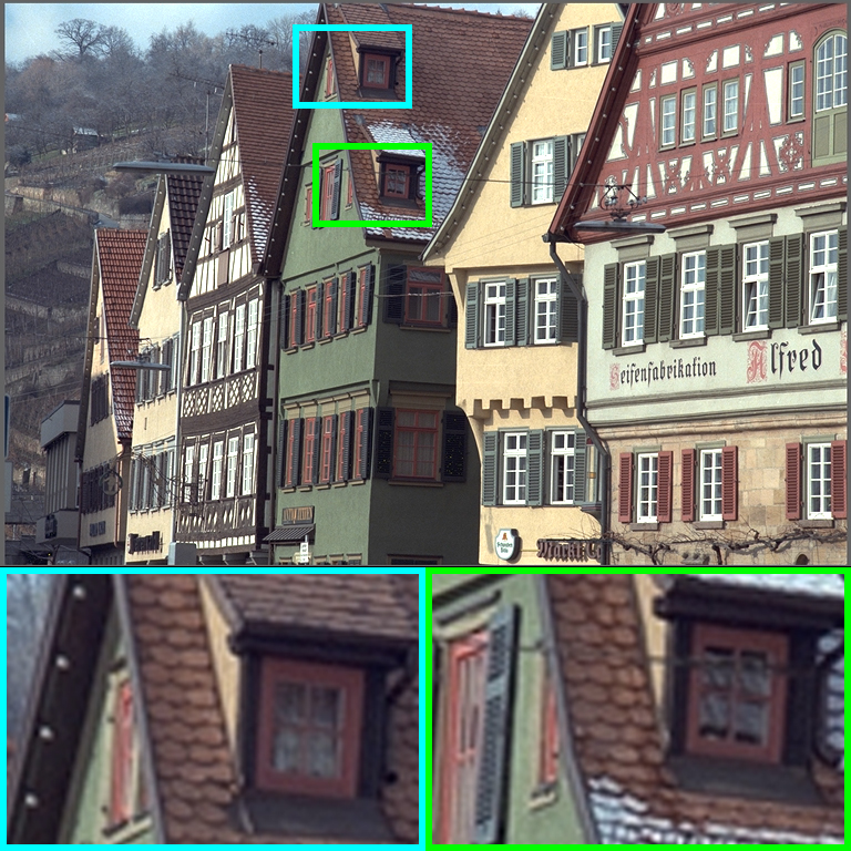
(a) Ground Truth

(b) Noisy: 20.73, 0.6697

(c) CBM3D: 29.27, 0.8766

(d) LRQA: 27.94, 0.8583

(e) ​​​MCWNNM:31.26, 0.9277

(f) ​​​MCWSNM:31.28, 0.9269

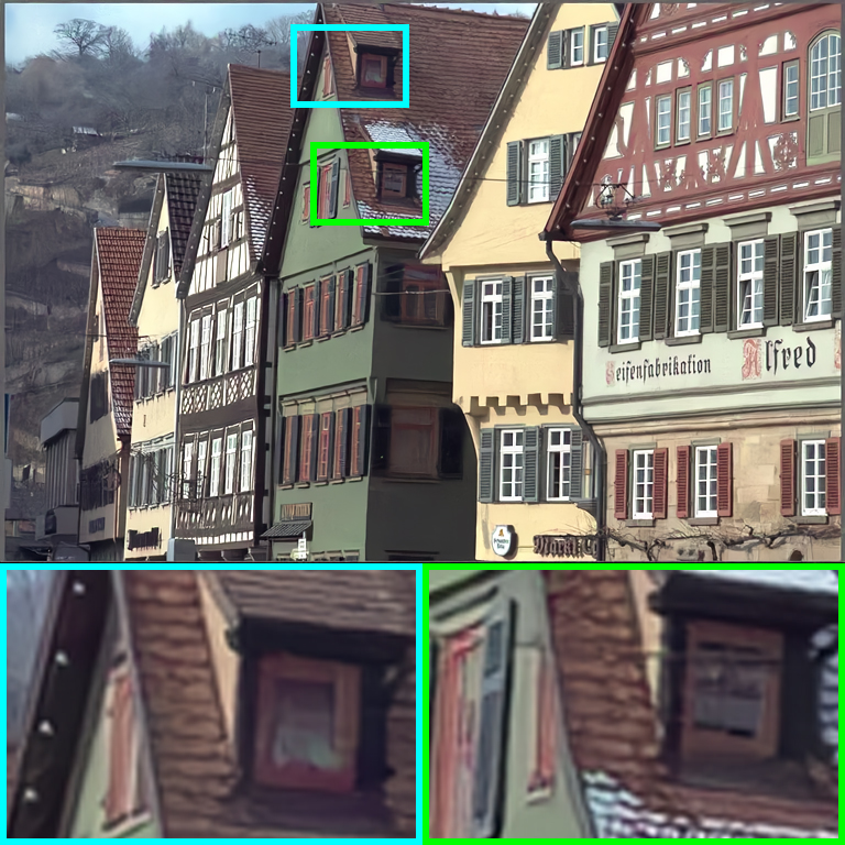
(g) FFDNet: 30.33, 0.9029

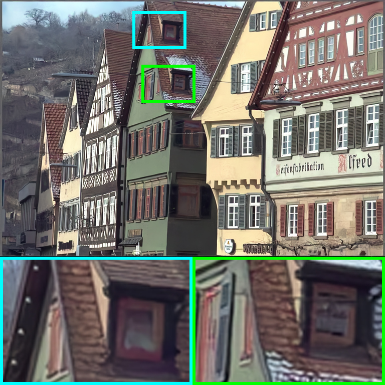
(h) DnCNN: 30.45, 0.9041

(i) NNFNM: 31.45, 0.9289

(j) DtNFM: 31.66, 0.9324

Figure 6: Denoised results on “kodim08.png” under the noise $[\sigma_{r};\sigma_{g};\sigma_{b}]=[20;35;5]$.

(a) Ground Truth

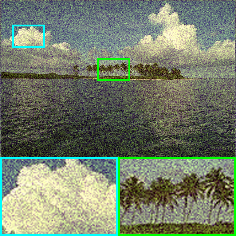
(b) Noisy: 20.73, 0.4560

(c) CBM3D: 31.41, 0.8159

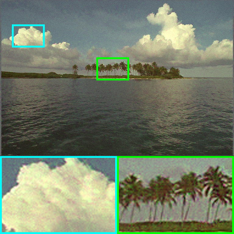
(d) LRQA: 30.38, 0.7822

(e) ​​​MCWNNM:34.15, 0.8976

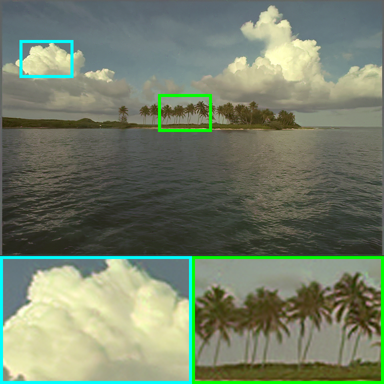
(f) ​​​MCWSNM:34.11, 0.8996

(g) FFDNet: 32.88, 0.8780

(h) DnCNN: 32.80, 0.8766

(i) NNFNM: 34.34, 0.8984

(j) DtNFM: 34.52, 0.9051

Figure 7: Denoised results on “kodim16.png” under the noise $[\sigma_{r};\sigma_{g};\sigma_{b}]=[20;35;5]$.

(a) Ground Truth

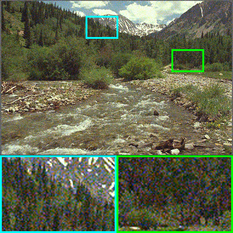
(b) Noisy: 17.46, 0.5251

(c) CBM3D: 25.45, 0.7100

(d) LRQA: 24.45, 0.6894

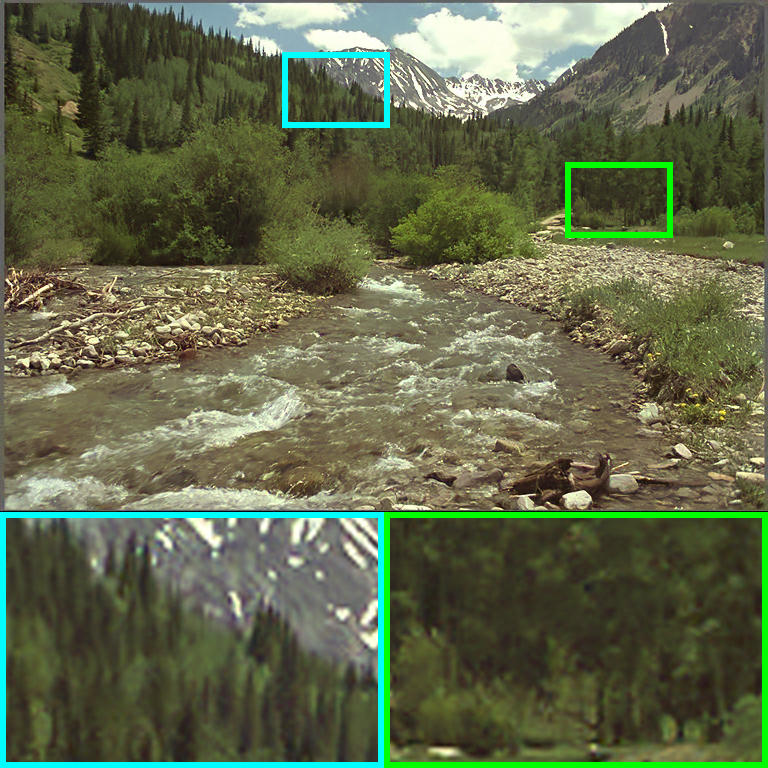
(e) ​​​MCWNNM:27.47, 0.8164

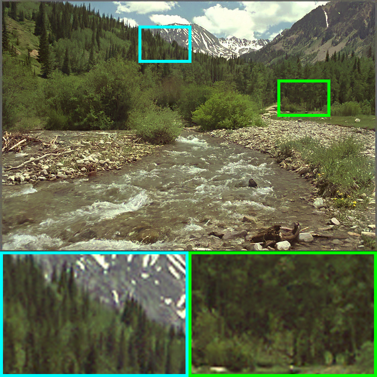
(f) ​​​MCWSNM:27.25, 0.8049

(g) FFDNet: 26.37, 0.7685

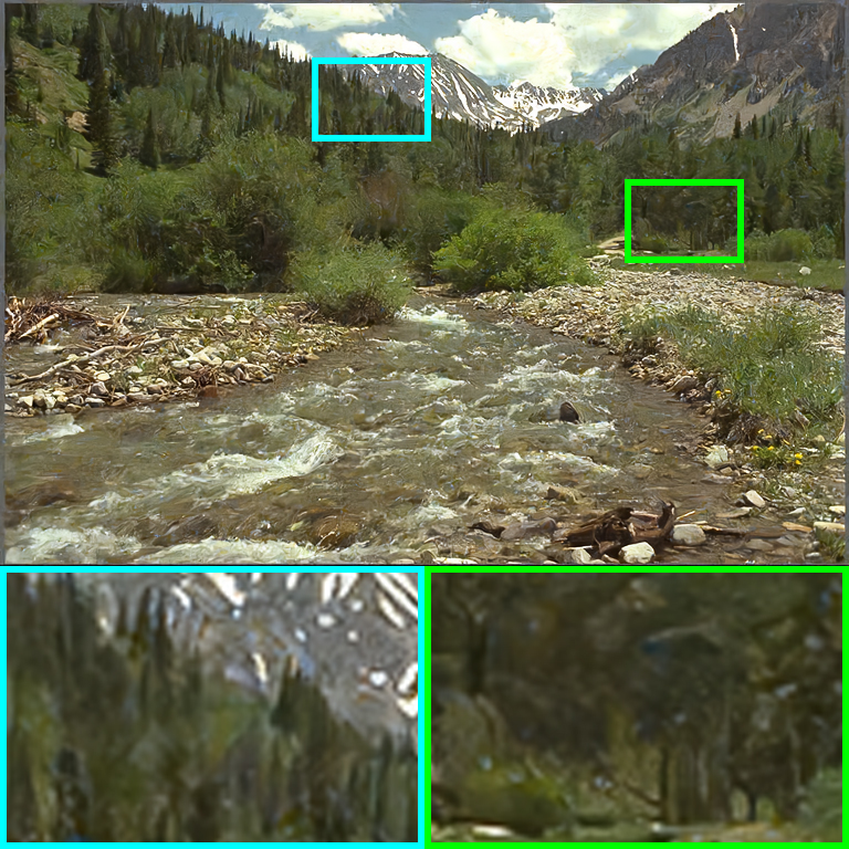
(h) DnCNN: 26.37, 0.7758

(i) NNFNM: 27.18, 0.8130

(j) DtNFM: 27.89, 0.8233

Figure 8: Denoised results on “kodim13.png” under the noise $[\sigma_{r};\sigma_{g};\sigma_{b}]=[30;10;50]$.

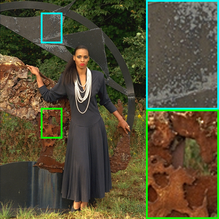
(a) Ground Truth

(b) Noisy: 17.46, 0.3967

(c) CBM3D: 27.54, 0.7386

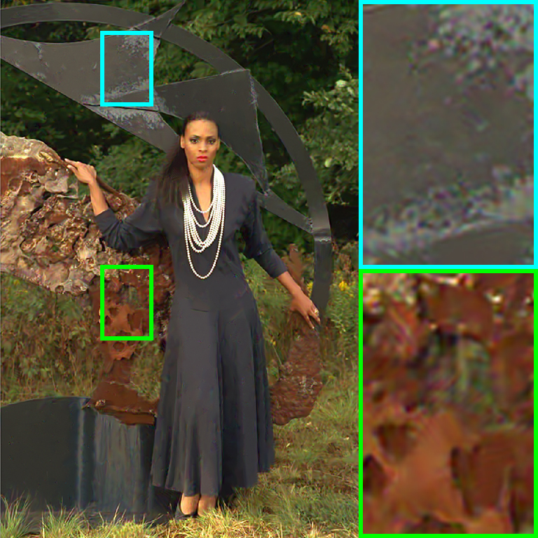
(d) LRQA: 26.21, 0.7388

(e) ​​​MCWNNM:29.61, 0.8287

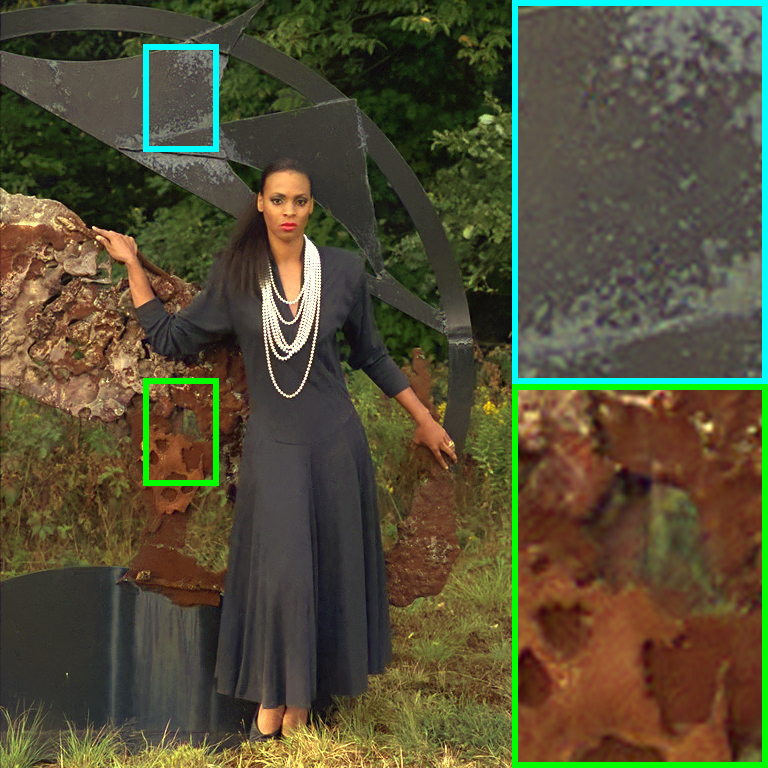
(f) ​​​MCWSNM:29.42, 0.8230

(g) FFDNet: 28.63, 0.8031

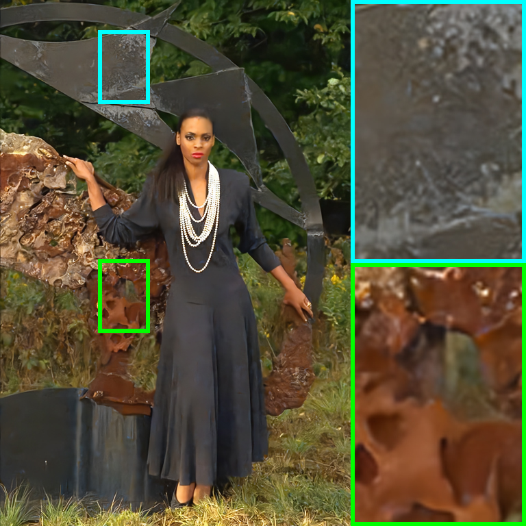
(h) DnCNN: 28.70, 0.8080

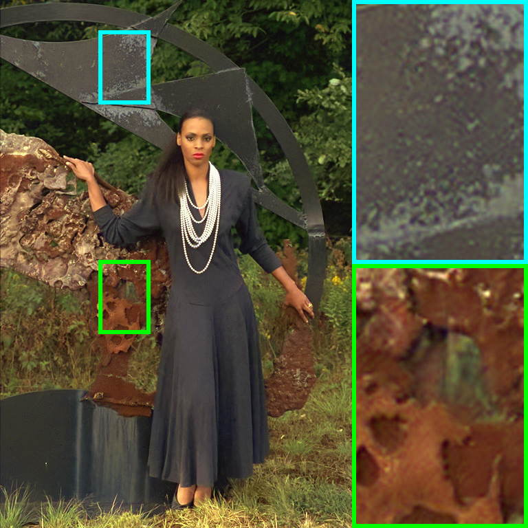
(i) NNFNM: 29.49, 0.8276

(j) DtNFM: 29.91, 0.8352

Figure 9: Denoised results on “kodim18.png” under the noise $[\sigma_{r};\sigma_{g};\sigma_{b}]=[30;10;50]$.

The visual comparisons are shown in Fig. 6 $\sim$ Fig. 9. It can be observed that the proposed DtNFM not only removes the noise completely, but also makes better protection for the textures, edges and details. In contrast, CBM3D generates artifacts and LRQA remains the noise. In Fig. 8, DtNFM achieves better protection on the complex edges of trees and shrub. In the denoised images generated by FFDNet and DnCNN, however, those edges are distorted and large amount of false color is generated. In Fig. 9, both the textures of the sculpture and the detailed structure of the stone are well recovered by DtNFM. While LRQA and MCWSNM suffer from oversmoothing and generate false colors. In summary, the proposed DtNFM method achieves the best performance in both numerical results and visual quality.

4.2 Removing Synthetic Noise with Cross-Channel Difference and Spatial Variation

In the most previous section, the noise standard deviation $[\sigma_{r};\sigma_{g};\sigma_{b}]$ is constant over all pixels. However, in practical applications, the noise often demonstrates spatial variation. Therefore, in this section we consider the noise possessing both cross-channel difference and spatial variation. To synthesize such kind of noise, we first choose the upper-bounds of the noise standard deviation, denoted as $[\bar{\sigma}_{r};\bar{\sigma}_{g};\bar{\sigma}_{b}]$. Then, we generate a map $\mathcal{M}(x,y)$ where $x,y\in\{1,\cdots,512\}$, as shown in Fig. 5c. Note that $\mathcal{M}(\cdot,\cdot)\in[0,1]$. A point $(x,y,\mathcal{M}(x,y))$ means that for the pixel at $x$th row and $y$th column, the noise standard deviation imposed on it is $\mathcal{M}(x,y)\odot[\bar{\sigma}_{r};\bar{\sigma}_{g};\bar{\sigma}_{b}]$. For all competing methods, the input noise standard deviation for each color channel is

$$\sigma_{c}=\frac{\bar{\sigma}_{c}}{512^{2}}\sum_{j=1}^{512}\sum_{i=1}^{512}\mathcal{M}(x,y),$$ (55)

where $c\in\{r,g,b\}$.

The ground truth images are still taken from Kodak24 data set. The images are cropped to $512\times 512$ pixels in order to match the size of $\mathcal{M}$. The upper-bounds of noise standard deviation $[\bar{\sigma}_{r};\bar{\sigma}_{g};\bar{\sigma}_{b}]$ are set as $[30;35;40]$. Two cases of DtNFM method are conducted. In the first case, the DtNFM method is unaware of the distribution of the noise standard deviation, i.e., the map $\mathcal{M}$. Consequently, DtNFM has to assume that the noise has no spatial variation. Such assumption do will reduce the performance of DtNFM, since the weight matrix $\mathbf{S}$ can not be constructed correctly. This case is denoted as “DtNFM_b” (blind). In the second case, the map $\mathcal{M}$ is learned by DtNFM. Therefore, the spatial variation of noise can be fully modeled and utilized. And this case is denoted as “DtNFM_a” (aware). For both DtNFM_b and DtNFM, we set $\lambda=1.85,\rho=0.50,\alpha=1$, and $t=7$. Other parameters are kept the same as those in section 4.1.

Table 4:
PSNR(dB) and SSIM results for all competing methods in the spatially variant noise experiments.

	​​CBM3D	​​MCWNNM	​​MCWSNM	​​FFDNet	​​DnCNN	​​NNFNM	​​DtNFM_b	​​DtNFM_a
#	​​PSNR SSIM	​​PSNR SSIM	​​PSNR SSIM	​​PSNR SSIM	​​PSNR SSIM	​​PSNR SSIM	​​PSNR SSIM	​​PSNR SSIM
1	​​ 31.73 0.9280	​​ 30.13 0.8685	​​ 29.41 0.8374	​​ 32.29 0.9137	​​ 31.95 0.9094	​​ 32.25 0.9277	​​ 32.46 0.9296	​​ 33.15 0.9455
2	​​ 32.39 0.8578	​​ 32.65 0.8436	​​ 32.59 0.8364	​​ 33.00 0.8397	​​ 32.73 0.8316	​​ 33.43 0.8775	​​ 35.23 0.9071	​​ 35.71 0.9108
3	​​ 33.95 0.8619	​​ 34.97 0.9107	​​ 35.44 0.9181	​​ 35.08 0.8997	​​ 34.62 0.9001	​​ 33.02 0.8749	​​ 37.73 0.9419	​​ 37.87 0.9382
4	​​ 32.70 0.8615	​​ 33.37 0.8575	​​ 33.41 0.8534	​​ 33.60 0.8535	​​ 33.08 0.8438	​​ 33.04 0.8654	​​ 36.23 0.9136	​​ 36.50 0.9172
5	​​ 32.14 0.9407	​​ 31.25 0.9221	​​ 30.94 0.9116	​​ 32.93 0.9422	​​ 32.65 0.9378	​​ 32.09 0.9473	​​ 33.13 0.9574	​​ 33.61 0.9639
6	​​ 32.39 0.8989	​​ 31.66 0.8681	​​ 31.32 0.8557	​​ 33.01 0.8893	​​ 32.73 0.8833	​​ 32.48 0.9059	​​ 33.52 0.9208	​​ 34.39 0.9287
7	​​ 33.62 0.8930	​​ 34.32 0.9304	​​ 34.63 0.9362	​​ 35.01 0.9356	​​ 34.49 0.9318	​​ 32.97 0.9125	​​ 36.15 0.9452	​​ 37.12 0.9547
8	​​ 32.25 0.9208	​​ 31.66 0.9168	​​ 31.35 0.9129	​​ 32.53 0.9233	​​ 32.34 0.9198	​​ 32.12 0.9277	​​ 32.97 0.9405	​​ 33.87 0.9468
9	​​ 33.39 0.8559	​​ 34.27 0.9084	​​ 34.62 0.9137	​​ 34.88 0.9100	​​ 34.42 0.9067	​​ 32.82 0.8770	​​ 36.08 0.9323	​​ 36.79 0.9334
10	​​ 33.42 0.8498	​​ 34.09 0.8940	​​ 34.44 0.8999	​​ 34.65 0.8941	​​ 34.16 0.8885	​​ 32.22 0.8604	​​ 35.99 0.9187	​​ 35.95 0.9296
11	​​ 32.14 0.9055	​​ 31.73 0.8683	​​ 31.51 0.8574	​​ 32.82 0.8790	​​ 32.47 0.8725	​​ 32.09 0.9040	​​ 33.38 0.9263	​​ 34.33 0.9294
12	​​ 33.12 0.8632	​​ 33.63 0.8680	​​ 33.72 0.8645	​​ 33.89 0.8685	​​ 33.33 0.8572	​​ 33.16 0.8742	​​ 35.98 0.9179	​​ 36.46 0.9213
13	​​ 31.25 0.9428	​​ 29.35 0.8576	​​ 28.63 0.8141	​​ 31.80 0.9204	​​ 31.41 0.9156	​​ 31.29 0.9423	​​ 30.89 0.9332	​​ 32.60 0.9535
14	​​ 31.98 0.9048	​​ 31.06 0.8586	​​ 30.59 0.8389	​​ 32.49 0.8868	​​ 32.18 0.8802	​​ 32.01 0.9082	​​ 33.17 0.9235	​​ 33.76 0.9338
15	​​ 32.45 0.8672	​​ 32.78 0.8579	​​ 32.66 0.8504	​​ 33.05 0.8480	​​ 32.79 0.8489	​​ 32.71 0.8747	​​ 34.82 0.9107	​​ 35.45 0.9161
16	​​ 32.99 0.8748	​​ 32.69 0.8644	​​ 32.55 0.8564	​​ 33.71 0.8820	​​ 33.23 0.8719	​​ 32.34 0.8755	​​ 34.96 0.9136	​​ 35.81 0.9237
17	​​ 32.72 0.8851	​​ 32.99 0.8834	​​ 32.95 0.8794	​​ 33.59 0.8875	​​ 33.22 0.8825	​​ 32.62 0.8900	​​ 34.62 0.9290	​​ 36.11 0.9337
18	​​ 32.10 0.8815	​​ 31.10 0.8553	​​ 30.72 0.8403	​​ 32.75 0.8868	​​ 32.44 0.8822	​​ 32.53 0.8928	​​ 33.00 0.9052	​​ 33.75 0.9189
19	​​ 32.50 0.9135	​​ 32.73 0.9083	​​ 32.67 0.9023	​​ 33.65 0.9168	​​ 33.28 0.9112	​​ 32.43 0.9177	​​ 34.82 0.9394	​​ 35.29 0.9446
20	​​ 33.33 0.8672	​​ 33.49 0.8901	​​ 33.51 0.8898	​​ 34.50 0.9065	​​ 34.75 0.9104	​​ 32.77 0.8865	​​ 35.31 0.9244	​​ 36.21 0.9372
21	​​ 32.50 0.8873	​​ 31.93 0.8945	​​ 31.68 0.8902	​​ 33.45 0.9095	​​ 33.12 0.9059	​​ 31.81 0.8903	​​ 33.10 0.9156	​​ 34.05 0.9314
22	​​ 32.23 0.8734	​​ 32.03 0.8541	​​ 31.68 0.8402	​​ 32.93 0.8700	​​ 32.57 0.8620	​​ 32.76 0.8853	​​ 33.86 0.9077	​​ 35.06 0.9190
23	​​ 33.62 0.8516	​​ 34.61 0.8957	​​ 35.08 0.9063	​​ 34.74 0.8954	​​ 34.22 0.8898	​​ 32.75 0.8657	​​ 36.39 0.9310	​​ 37.65 0.9314
24	​​ 32.34 0.8998	​​ 32.23 0.8978	​​ 31.98 0.8896	​​ 33.32 0.9114	​​ 32.93 0.9059	​​ 32.48 0.9078	​​ 33.47 0.9253	​​ 34.90 0.9441
Avg	​​ 32.64 0.8869	​​ 32.53 0.8823	​​ 32.42 0.8748	​​ 33.49 0.8946	​​ 33.13 0.8895	​​ 32.51 0.8955	​​ 34.47 0.9254	​​ 35.27 0.9336

The PSNR and SSIM results are listed in Table 4. The results of the LRQA method are omitted due to space limit. The best results are highlighted in bold and the second-best results are underlined. As can be seen, the DtNFM method achieves the highest PSNR on 23 images, and the highest SSIM on 23 images. Even being unaware of the distribution of noise standard deviation, the DtNFM_b still outperforms other competing methods, achieving the second-highest PSNR on 21 images, and the second-highest SSIM on 22 images. For a fair comparison, we will focus on DtNFM_b, since other competing methods are also unaware of the spatial variation. The average improvements of DtNFM_b over other methods are listed in the third row of Table 3. As can be seen, the superiority of DtNFM_b is significant. It is worth noticing that MCWNNM, MCWSNM and NNFNM do can handle the noise spatial variation to some extent. However, they are not flexible enough since they ignore the noise variation between those patches in the same group. In other words, they can only handle the noise variation between patch matrices. This inflexibility is fully exposed by the experiments in this section. As shown in Table 4, those three methods are outperformed by FFDNet and DnCNN. This drawback is significantly alleviated in the proposed DtNFM method.

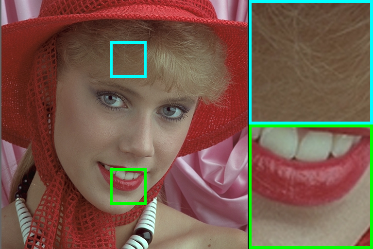
(a) Ground Truth

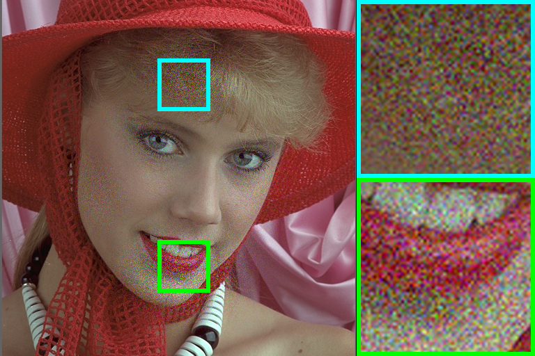
(b) Noisy: 29.65, 0.8297

(c) CBM3D: 32.70 0.8615

(d) ​​​MCWNNM:33.37 0.8575

(e) ​​​MCWSNM:33.41 0.8534

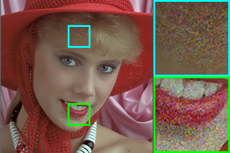
(f) FFDNet: 33.08 0.8438

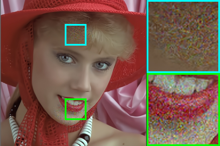
(g) DnCNN: 33.60 0.8535

(h) NNFNM: 33.04 0.8654

(i) DtNFM_b: 36.23 0.9136

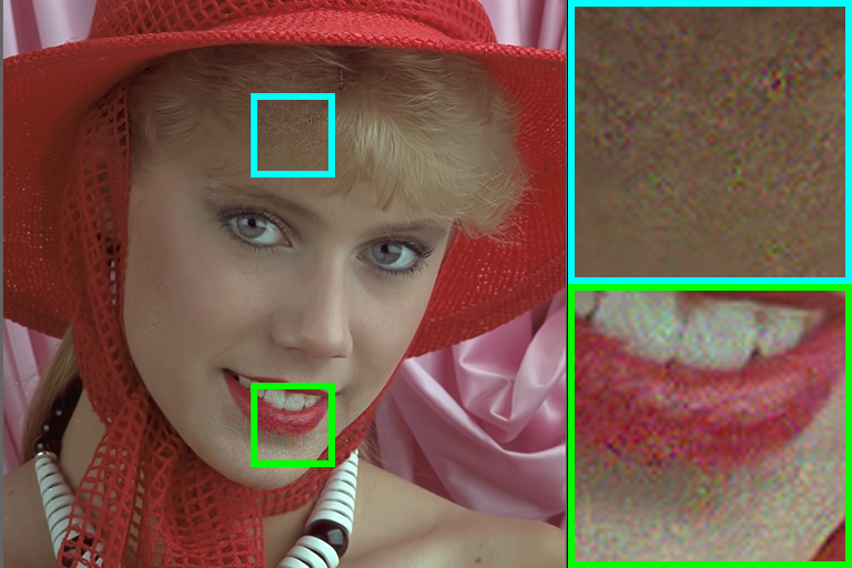
(j) DtNFM: 36.50, 0.9172

Figure 10: Visual results of “kodim04.png” under the noise with spatial variation.

(a) Ground Truth

(b) Noisy: 29.65, 0.8297

(c) CBM3D: 33.12 0.8632

(d) ​​​MCWNNM:33.63 0.8680

(e) ​​​MCWSNM:33.72 0.8645

(f) FFDNet: 33.33 0.8572

(g) DnCNN: 33.89 0.8685

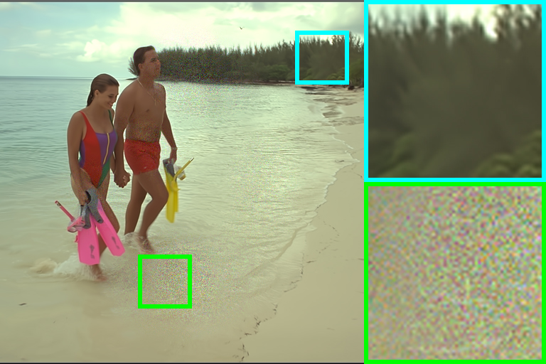
(h) NNFNM: 33.16 0.8742

(i) DtNFM_b: 35.98 0.9179

(j) DtNFM: 36.46, 0.9213

Figure 11: Visual results of “kodim12” under the noise with spatial variation.

The visual comparisons are shown in Fig. 10 and Fig. 11. In Fig. 10, both DtNFM_b and DtNFM_a remove the noise completely. While DtNFM_a preserves more details, such as the hair and mouth. In contrast, other methods remain too much noise. In Fig. 10, all competing methods remain noise to some extent. While DtNFM_b and DtNFM_a remove more noise than other methods. Moreover, DtNFM_b and DtNFM_a do not oversmooth the image, which is indicated by the trees at the top-right corner. In summary, the proposed DtNFM method achieves a more rational balance between noise removal and detail protection.

Table 5:
PSNR(dB) and SSIM results for all competing methods in the real-world noise experiments.

	​​CBM3D	​​LRQA	​​MCWNNM	​​MCWSNM	​​FFDNet	​​DnCNN	​​NNFNM	​​DtNFM
#	​​PSNR SSIM	​​PSNR SSIM	​​PSNR SSIM	​​PSNR SSIM	​​PSNR SSIM	​​PSNR SSIM	​​PSNR SSIM	​​PSNR SSIM
1	​​38.75 0.9688	​​34.68 0.9739	​​38.37 0.9678	​​36.95 0.9785	​​39.40 0.9732	​​40.10 0.9775	​​41.24 0.9835	​​41.39 0.9837
2	​​35.52 0.9407	​​33.60 0.9465	​​35.37 0.9359	​​35.25 0.9541	​​37.02 0.9522	​​37.04 0.9547	​​37.25 0.9607	​​37.26 0.9599
3	​​35.69 0.9583	​​33.48 0.9568	​​34.91 0.9478	​​35.31 0.9632	​​36.53 0.9620	​​36.40 0.9605	​​36.96 0.9683	​​37.08 0.9677
4	​​33.84 0.9220	​​32.85 0.9403	​​34.98 0.9484	​​34.02 0.9482	​​34.97 0.9512	​​35.18 0.9557	​​35.54 0.9600	​​35.47 0.9592
5	​​34.66 0.9050	​​33.57 0.9335	​​35.95 0.9293	​​34.81 0.9400	​​36.73 0.9553	​​36.65 0.9521	​​37.10 0.9584	​​37.12 0.9583
6	​​36.22 0.9062	​​34.56 0.9621	​​41.15 0.9799	​​36.53 0.9650	​​41.02 0.9840	​​39.82 0.9722	​​41.27 0.9874	​​41.24 0.9872
7	​​36.63 0.9297	​​35.45 0.9562	​​37.99 0.9575	​​37.15 0.9623	​​38.66 0.9598	​​39.10 0.9675	​​39.35 0.9687	​​39.26 0.9676
8	​​37.32 0.9296	​​35.50 0.9698	​​40.36 0.9767	​​37.70 0.9733	​​41.53 0.9809	​​41.26 0.9798	​​41.84 0.9816	​​41.96 0.9817
9	​​36.31 0.9006	​​35.36 0.9458	​​38.30 0.9427	​​37.22 0.9521	​​38.80 0.9427	​​39.09 0.9517	​​39.70 0.9556	​​39.54 0.9554
10	​​34.40 0.8647	​​35.49 0.9402	​​39.01 0.9637	​​36.73 0.9457	​​40.15 0.9765	​​37.86 0.9514	​​39.66 0.9749	​​40.21 0.9777
11	​​33.54 0.8743	​​34.01 0.9194	​​36.75 0.9477	​​35.03 0.9265	​​37.61 0.9578	​​35.97 0.9385	​​37.84 0.9586	​​37.59 0.9557
12	​​34.24 0.8352	​​34.78 0.9353	​​39.06 0.9544	​​36.73 0.9464	​​41.18 0.9773	​​38.08 0.9493	​​42.77 0.9832	​​42.46 0.9828
13	​​30.64 0.7691	​​30.48 0.8457	​​34.61 0.9206	​​33.07 0.9075	​​34.13 0.9148	​​33.63 0.8988	​​35.18 0.9371	​​35.39 0.9367
14	​​30.88 0.8473	​​30.02 0.8750	​​33.21 0.9369	​​32.25 0.9247	​​33.66 0.9376	​​33.35 0.9311	​​34.06 0.9471	​​34.07 0.9466
15	​​30.48 0.8146	​​30.69 0.8619	​​33.22 0.9118	​​32.08 0.8864	​​33.69 0.9196	​​32.62 0.8951	​​34.14 0.9245	​​34.19 0.9215
Avg	​​34.61 0.8911	​​33.63 0.9308	​​36.88 0.9481	​​35.39 0.9449	​​37.67 0.9563	​​37.08 0.9491	​​38.26 0.9633	​​38.28 0.9628

4.3 Removing Real-World Noise

CC15 data set has 15 real-world noisy images and their noise-free versions. The noise-free images are obtained by averaging each pixel from 500 images shot on the same scene under same camera settings. Therefore, they can be practically used as ground truth. With them, the quantitative comparison can be carried out since PSNR and SSIM can be calculated. For each noisy image, the noise standard deviations $[\sigma_{r};\sigma_{g};\sigma_{b}]$ are estimated by a state-of-the-art noise estimation method [42]. Then, competing methods denoise the image under the assumption that the noise possess no spatial variation. For DtNFM method, we tune $\lambda=2.3$, $\rho=0.9,t=0$ and $\alpha=1.8$. Other parameters are kept the same as those in section 4.1. We remove the restriction of using a fixed number of iterations, i.e., $\theta$, to denoise all the images.

(a) Ground Truth

(b) Noisy: 35.71, 0.8839

(c) CBM3D: 37.32 0.9296

(d) LRQA: 37.32 0.9296

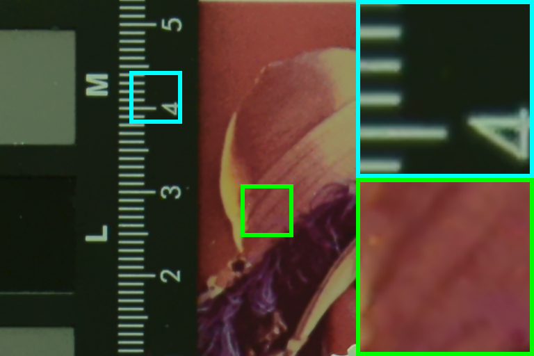
(e) ​​​MCWNNM:40.36 0.9767

(f) ​​​MCWSNM:37.70 0.9733

(g) FFDNet: 41.53 0.9809

(h) DnCNN: 41.26 0.9798

(i) NNFNM: 41.84 0.9816

(j) DtNFM: 41.96, 0.9817

Figure 12: Visual results of image “#8”.

(a) Ground Truth

(b) Noisy: 33.26, 0.8167

(c) CBM3D: 34.40 0.8647

(d) LRQA: 35.49 0.9402

(e) ​​​MCWNNM:39.01 0.9637

(f) ​​​MCWSNM:36.73 0.9457

(g) FFDNet: 40.15 0.9765

(h) DnCNN: 37.86 0.9514

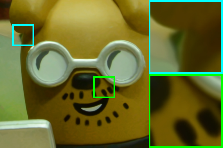
(i) NNFNM: 39.66 0.9749

(j) DtNFM: 40.21, 0.9777

Figure 13: Visual results of image “#10”.

The PSNR and SSIM results are listed in Table 5. The best results are bolded and the second-best results are underlined.  As can be seen, DtNFM method achieves the highest PSNR on 9 images and the second-highest on 5 images. And DtNFM achieves the highest SSIM on 3 images and the second-highest on 11 images. On average, the improvements of DtNFM over other methods are listed in the bottom row of Table 3. DtNFM fails to achieve the highest average SSIM, slightly underperformed the NNFNM method. However, DtNFM still achieves the highest average PSNR. The visual comparisons are shown in Fig. 12 and Fig. 13. DtNFM generates satisfactory visual quality since it removes the noise fully. In contrast, CBM3D, LRQA and DnCNN remain the noise. All competing methods do not over-smooth the images and generate no artifacts, since the noise pollution is mild.

4.4 The Impact of the Hyper-parameters $\lambda$ and $t$

To give an empirical basis for modifying the hyper-parameters $\lambda$ and $t$, we analysis their impacts on the model performance. All the test images are taken from Kodak24 data set. The noisy observations are generated by the noise with $[\sigma_{r};\sigma_{g};\sigma_{b}]=[30;10;50]$ and no spatial variation. All the parameters are fixed but $\lambda$ and $t$.

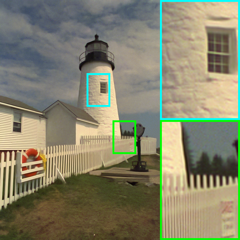
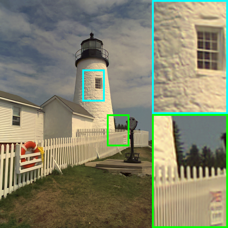
	$\quad\lambda=0.001\quad\quad\quad\quad\lambda=1\quad\quad\quad\quad\ \lambda=1000$
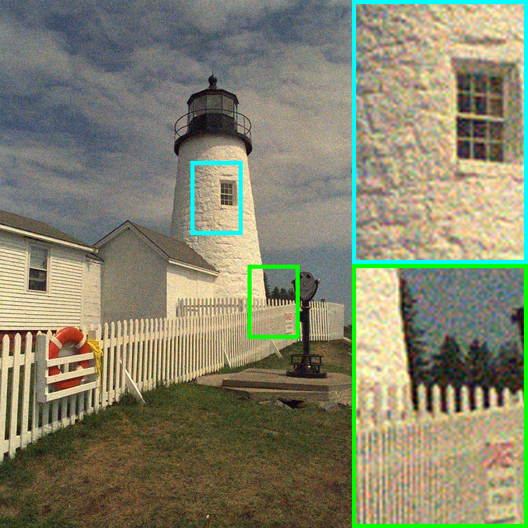
$t=0$	(a) 22.19, 0.4347 (b) ​​31.42, 0.8501 (c) ​​27.68, 0.7281
$t=1$	(d) 22.19, 0.4347 (e) 31.67, 0.8561 (f) 28.68, 0.7475
$t=2$	(g) 22.19, 0.4347 (h) 31.82, 0.8597 (i) 29.36, 0.7665
$t=3$	(j) 22.19, 0.4347 (k) 31.97, 0.8611 (l) 29.64, 0.7838

Figure 14: Visual results of “kodim19.png” with different values of $\lambda$ and $t$.

The regularization parameter $\lambda$ is actually the most important parameter. It controls the regularization effects of the objective function in (13), and further controls the trade-off between noise removal and over-smoothing. Concretely, as it becomes too small, a resultant DtNFM model will suffer from overfitting since it mostly minimize the loss term in (13). Consequently, the output image will contain too much noise, as shown in Fig. 14a, Fig. 14d, Fig. 14g, and Fig. 14j. On the contrary, as $\lambda$ becomes too large, a resultant DtNFM model may suffer from underfitting since it minimize the regularization term too much. Consequently, the output image may be over-smoothed, as shown in Fig. 14c. However, the problem of over-smoothing will be alleviated as $t$ becomes larger, as shown in Fig. 14d, Fig. 14g, and Fig. 14j. As $t$ becomes larger, the $t$ most dominant rank components of the estimated patch matrix $\mathbf{X}$ are bound to get zero penalty, even $\lambda\rightarrow+\infty$. Therefore, the more information can be preserved.

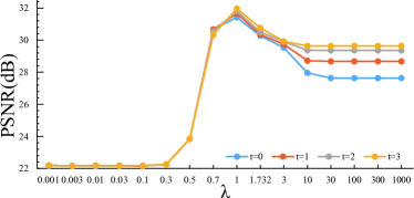
(a)

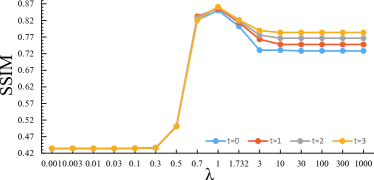
(b)

Figure 15: PSNR and SSIM results of “kodim19.png” on the grid of values of $\lambda$ and $t$.

Although a larger $t$ can protect the image from over-smoothing, the resultant DtNFM model is still inadequate to be performant. As shown in Fig. 15, suboptimal PSNR and SSIM will be obtained when $\lambda$ is too large. While the optimal values of $\lambda$ are always around 1, regardless of the value of $t$. Therefore, the modification of $\lambda$ entails at least a line search.

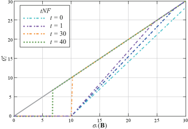
Figure 16: The shrinkage functions of the proximal operator (31) with $\tau=10$.

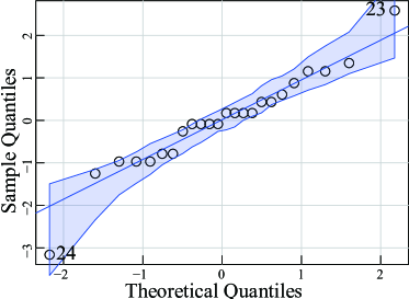
Figure 17: Test the normality via the Q-Q plot.

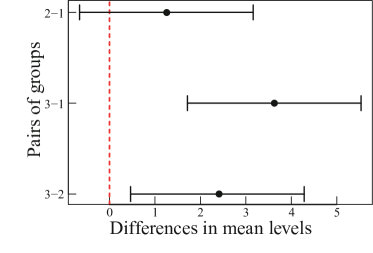
Figure 18: Multiple comparisons between all pairs.

Parameter $t\in\mathbb{N}$ impacts the model performance, since it controls the shrinkage on the estimated patch matrix $\mathbf{X}$. Fig. 16 shows the shrinkage performed by the tNF regularizer, i.e., the proximal operator (31). Intuitively, as $t$ becomes larger, more singular values would be preserved. Therefore, the choice of $t$ should be judicious so that the model performane can be improved.

We give an empirical choice method of $t$ by analyzing the initial value of SSIM, i.e., the SSIM of the input noisy image. Denote the initial SSIM as $SSIM_{0}$. Given a noisy image, the higher its $SSIM_{0}$ is, a larger $t$ is preferred. This argument is verified by resorting to the analysis of variance (ANOVA). Concretely, we first sort the $SSIM_{0}$ of 24 noisy images in an ascending order. Based on the order, the 24 noisy images are broke up into 3 groups, as shown in Table 6. To perform ANOVA, the dependant variable, i.e., $t$, has to be normally distributed and have an equal variance in each group. The normality assumption can be assessed via the Q-Q plot, which is provided in Fig. 16. As can be seen, the normality assumption is met since all of the points fall within the 95% confidence envelope, and the slope of the main diagonal is closed to 1. The equality of variances can be checked via the Barlett’s test. And the results ($p=0.165$) suggests that the variances in three groups do not differ significantly.

The results of ANOVA are shown in Table 7. As can be seen, the best $t$ for three groups are not equal since $p<0.05$. Although the multiple comparisons in Fig. 17 demonstrate that the averages of “best $t$” in group 1 and 2 are not significantly different, it is still easy to find the positive correlation between $SSIM_{0}$ and “best $t$”.

Table 6:
Grouping results of the 24 test images.

Group 1	Image#	23	3	12	20	2	15	9	10
	$SSIM_{0}$	0.2523	0.2578	0.2687	0.2754	0.2763	0.2785	0.2885	0.2930	Avg($t$)	Std($t$)
	Best $t$	2	2	3	3	3	4	3	5	3.125	0.991
Group 2	Image#	4	17	16	7	22	11	21	19
	$SSIM_{0}$	0.2962	0.3060	0.3123	0.3320	0.3390	0.3541	0.3592	0.3636	Avg($t$)	Std($t$)
	Best $t$	3	3	4	3	5	6	6	5	4.375	1.303
Group 3	Image#	6	18	24	14	1	5	13	8
	$SSIM_{0}$	0.3895	0.3967	0.3989	0.4037	0.4783	0.4888	0.5251	0.5418	Avg($t$)	Std($t$)
	Best $t$	5	7	8	7	7	7	10	3	6.750	2.053

Table 7:
The table of ANVOA.

Source	Sum of Squares	Degrees of Freedom	Mean Square	$F$	$p$
Inter-group	67.1258	2	33.5629	20.8604	$\mathbf{1.2764\times 10^{-5}}$
Within-group	32.1786	20	1.6089
Total	99.3044	22

5 Conclusion

In this paper, the DtNFM model was proposed and applied to color image denoising via integrating with the NSS prior. The DtNFM model possesses two advantiges. On the one hand, it can fully model and utilize the cross-channel difference and the spatial variation of noise. On the other hand, it can provide flexible treatments for different rank components, and further give a close approximation to the underlying low-rank matrix. To solve the resultant optimization problem, an accurate and effective algorithm was proposed by exploiting the framework of ADMM. Importantly, we mathematically proved the global optima of all subproblems can be obtained in closed-form. The convergence guarantee was established. Extensive experiments are carried out on the synthetic noise, spatially variant noise, and real-world noise images, respectively. The results demonstrated that the proposed method outperforms many state-of-the-art color image denoising methods.

6 Acknowledgements

This work is supported in part by the Sichuan Science and Technology Program under Grant 2021YFG0031 and Grant 22YSZH0021, in part by the Advanced Jet Propulsion Creativity Center Projects under Grant HKCX2022-01-022.

References

- [1] E. Shelhamer, J. Long, T. Darrell, Fully convolutional networks for semantic segmentation, IEEE Trans. Pattern Anal. Mach. Intell. 39 (4) (2017) 640–651.
- [2] S. Minaee, Y. Boykov, F. Porikli, A. Plaza, N. Kehtarnavaz, D. Terzopoulos, Image segmentation using deep learning: A survey, IEEE Trans. Pattern Anal. Mach. Intell. 44 (7) (2022) 3523–3542.
- [3] S. Li, W. Song, L. Fang, Y. Chen, P. Ghamisi, J. Benediktsson, Deep learning for hyperspectral image classification: An overview, IEEE Trans. Geosci. Remote Sensing 57 (9) (2019) 6690–6709.
- [4] Z. Zhao, P. Zheng, S. Xu, X. Wu, Object detection with deep learning: A review, IEEE Trans. Neural Netw. Learn. Syst. 30 (11) (2019) 3212–3232.
- [5] P. Hsiao, F. Chang, Y. Lin, Learning discriminatively reconstructed source data for object recognition with few examples, IEEE Trans. Image Process. 25 (2016) 3518–3532.
- [6] Z. Kong, X. Yang, Color image and multispectral image denoising using block diagonal representation, IEEE Trans. Image Process. 28 (9) (2019) 4247–4259.
- [7] Q. Wang, X. Zhang, Y. Wu, L. Tang, Z. Zha, Nonconvex weighted minimization based group sparse representation framework for image denoising, IEEE Signal Process. Lett. 24 (11) (2017) 1686–1690.
- [8] Z. Zha, X. Yuan, B. Wen, J. Zhou, C. Zhu, Group sparsity residual constraint with non-local priors for image restoration, IEEE Trans. Image Process. 29 (2020) 8960–8975.
- [9] S. Gu, Q. Xie, D. Meng, W. Zuo, X. Feng, L. Zhang, Weighted nuclear norm minimization and its applications to low level vision, Int. J. Comput. Vis. 121 (2017) 183–208.
- [10] Y. Xie, S. Gu, Y. Liu, W. Zuo, W. Zhang, L. Zhang, Weighted schatten -norm minimization for image denoising and background subtraction, IEEE Trans. Image Process. 25 (10) (2016) 4842–4857.
- [11] Y. Shan, D. Hu, Z. Wang, T. Jia, Multi-channel nuclear norm minus frobenius norm minimization for color image denoising, Signal Process. 207, art. no. 108959 (Jun. 2023).
- [12] K. Zhang, W. Zuo, Y. Chen, D. Meng, L. Zhang, Beyond a gaussian denoiser: Residual learning of deep cnn for image denoising, IEEE Trans. Image Process. 26 (7) (2017) 3142–3155.
- [13] K. Zhang, W. Zuo, L. Zhang, FFDNet: Toward a fast and flexible solution for cnn-based image denoising, IEEE Trans. Image Process. 27 (9) (2018) 4608–4622.
- [14] M. Zhao, G. Cao, X. Huang, L. Yang, Hybrid transformer-cnn for real image denoising, IEEE Signal Process. Lett. 29 (2022) 1252–1256.
- [15] F. Jia, L. Ma, Y. Yang, T. Zeng, Pixel-attention cnn with color correlation loss for color image denoising, IEEE Signal Process. Lett. 28 (2021) 1600–1604.
- [16] Y. Song, Y. Zhu, X. Du, Grouped multi-scale network for real-world image denoising, IEEE Signal Process. Lett. 27 (2020) 2124–2128.
- [17] A. Buades, B. Coll, J.-M. Morel, A non-local algorithm for image denoising, in: IEEE Conf. Comput. Vis. Pattern Recognit., Vol. 2, 2005, pp. 60–65.
- [18] S. Wang, L. Zhang, Y. Liang, Nonlocal spectral prior model for low-level vision, in: Proc. Asi. Conf. Comput. Vis., 2012, p. 231–244.
- [19] E.-J. Candès, B. Recht, Exact matrix completion via convex optimization, Found. Comput. Math. 9 (6) (2009) 717–772.
- [20] D. Donoho, Compressed sensing, IEEE Trans. Inf. Theory 52 (4) (2006) 1289–1306.
- [21] E.-J. Candes, M. B. Wakin, An introduction to compressive sampling, IEEE Signal Process. Mag. 25 (2) (2008) 21–30.
- [22] M. Fazel, H. Hindi, S. Boyd, A rank minimization heuristic with application to minimum order system approximation, in: Proc. American Control Conf., Vol. 6, 2001, pp. 4734–4739.
- [23] J. Cai, E.-J. Candès, Z. Shen, A singular value thresholding algorithm for matrix completion, SIAM J. Optim. 20 (4) (2010) 1956–1982.
- [24] K. Toh, S. Yun, An accelerated proximal gradient algorithm for nuclear norm regularized linear least squares problems, Pac. J. Optim. 6 (615-640) (2010) 15.
- [25] S. Ma, D. Goldfarb, L. Chen, Fixed point and bregman iterative methods for matrix rank minimization, Math. Program. 128 (2011) 321–353.
- [26] S. Gu, L. Zhang, W. Zuo, X. Feng, Weighted nuclear norm minimization with application to image denoising, in: Proc. IEEE Int. Conf. Comput. Vis., 2014, pp. 2862–2869.
- [27] Z. Zha, X. Yuan, B. Wen, J. Zhou, J. Zhang, C. Zhu, From rank estimation to rank approximation: Rank residual constraint for image restoration, IEEE Trans. Image Process. 29 (2020) 3254–3269.
- [28] Y. Chen, X. Xiao, Y. Zhou, Low-rank quaternion approximation for color image processing, IEEE Trans. Image Process. 29 (2020) 1426–1439.
- [29] Z. Wang, Y. Liu, X. Luo, J. Wang, C. Gao, D. Peng, W. Chen, Large-scale affine matrix rank minimization with a novel nonconvex regularizer, IEEE Trans. Neural Netw. Learn. Syst. 33 (9) (2022) 4661–4675.
- [30] Z. Wang, W. Wang, J. Wang, S. Chen, Fast and efficient algorithm for matrix completion via closed-form 2/3-thresholding operator, Neurocomputing 330 (2019) 212–222.
- [31] Z. Wang, D. Hu, X. Luo, W. Wang, J. Wang, W. Chen, Performance guarantees of transformed schatten-1 regularization for exact low-rank matrix recovery, Int. J. Mach. Learn. Cybern. 12 (2021) 3379–3395.
- [32] Z. Wang, C. Gao, X. Luo, M. Tang, J. Wang, W. Chen, Accelerated inexact matrix completion algorithm via closed-form q-thresholding operator, Int. J. Mach. Learn. Cybern. 11 (2020) 2327–2339.
- [33] Z. Liu, D. Hu, Z. Wang, J. Gou, T. Jia, Latlrr for subspace clustering via reweighted frobenius norm minimization, Expert Syst. Appl. 224 (2023) 119977.
- [34] Y. Wang, Q. Yao, J. Kwok, A scalable, adaptive and sound nonconvex regularizer for low-rank matrix learning, in: Int. World Wide Web Conf., 2021, p. 1798–1808.
- [35] W. Zuo, D. Meng, L. Zhang, X. Feng, D. Zhang, A generalized iterated shrinkage algorithm for non-convex sparse coding, in: Proc. IEEE Int. Conf. Comput. Vis., 2013, pp. 217–224.
- [36] K. Dabov, A. Foi, V. Katkovnik, K. Egiazarian, Color image denoising via sparse 3d collaborative filtering with grouping constraint in luminance-chrominance space, in: Proc. IEEE Int. Conf. Image Process., Vol. 1, 2007, pp. 313–316.
- [37] J. Xu, L. Zhang, D. Zhang, X. Feng, Multi-channel weighted nuclear norm minimization for real color image denoising, in: Proc. IEEE Int. Conf. Comput. Vis., 2017, pp. 1105–1113.
- [38] C. Huang, Z. Li, Y. Liu, T. Wu, T. Zeng, Quaternion-based weighted nuclear norm minimization for color image restoration, Pattern Recognition 128 (2022) 108665.
- [39] X. Huang, B. Du, W. Liu, Multichannel color image denoising via weighted schatten p-norm minimization, in: Proc. Int. Joint Conf. Artif. Intell., 2020, pp. 637–644.
- [40] M. Hong, Z. Luo, M. Razaviyayn, Convergence analysis of alternating direction method of multipliers for a family of nonconvex problems, SIAM J. Optim. 26 (1) (2016) 337–364.
- [41] B. Leung, G. Jeon, E. Dubois, Least-squares luma–chroma demultiplexing algorithm for bayer demosaicking, IEEE Trans. Image Process. 20 (7) (2011) 1885–1894.
- [42] G. Chen, F. Zhu, P. Heng, An efficient statistical method for image noise level estimation, in: Proc. IEEE Int. Conf. Comput. Vis., 2015, pp. 477–485.
- [43] S. Nam, Y. Hwang, Y. Matsushita, S. J. Kim, A holistic approach to cross-channel image noise modeling and its application to image denoising, in: Proc. IEEE Int. Conf. Comput. Vis., 2016, pp. 1683–1691.