A Graph-Prediction-Based Approach for Debiasing Underreported Data

Abstract

We present a novel Graph-based debiasing Algorithm for Underreported Data (GRAUD) aiming at an efficient joint estimation of event counts and discovery probabilities across spatial or graphical structures. This innovative method provides a solution to problems seen in fields such as policing data and COVID-$19$ data analysis. Our approach avoids the need for strong priors typically associated with Bayesian frameworks. By leveraging the graph structures on unknown variables $n$ and $p$, our method debiases the under-report data and estimates the discovery probability at the same time. We validate the effectiveness of our method through simulation experiments and illustrate its practicality in one real-world application: police 911 calls-to-service data.

Index Terms—  Graph signal separation, Data debiasing, Alternating minimization

1 Introduction

Bias in data collection is a prevalent issue in many real-world applications due to a variety of reasons. One common scenario is under-reporting, as elucidated by [1]. For example, police 911 calls-to-service reports, as [2] illustrates, potentially omitting a significant number of unrecorded incidents. Similarly, during the COVID-19 pandemic, data collection, as indicated by [3], only accounted for those individuals who tested positive, which overlooked asymptomatic individuals and those who hadn’t undergone testing, further perpetuating data bias.

The challenge in addressing underreporting data is that there exists a substantial identifiability issue. For instance, while the count of observed cases, denoted by $y$, is known, the count of unobserved instances is not uniquely determined. This is due to the fact that there are infinitely many solutions for the equation $y=np$ when only $y$ is known.

The problem of estimating the probability $p$ in a binomial Bin($n$, $p$) distribution when the number of trials $n$ is known has been thoroughly addressed in the classic statistical literature. However, the circumstance where both $n$ and $p$ are unknown is much harder and more interesting. This gives rise to the binomial $n$ problem [4]. In the realm of statistics, this problem is a well-known issue when it comes to one-dimensional cases. Traditionally, the approach to resolving it involves utilizing Bayesian methodologies, as detailed in works like [5, 6, 7, 8, 9]. However, this leads to the secondary challenge of selecting an appropriate prior.

Following the setting mentioned before, where there are $n$ possible events, each being observed with a probability $p$. We are then confronted with a count, $y$, which is modeled as a Binomial random variable, $\mbox{Binomial}(n,p)$. Our primary focus is on estimating the parameters $n$ and $p$ while relying exclusively on the observations of $y$. A significant complication arises from the fact that the expected value of $y$ is $np$. Although we mentioned the identifiability issue, we may utilize additional information to help circumvent the identifiability issue. This paper presents such a graph-prediction-based approach for debiasing underreported data called GRAUD.

1.1 Related work

The early studies on simultaneously estimating the parameters $n$ and $p$ were spearheaded byWhitaker [10], Fisher [11], and Haldane [12]. They introduced the Method of Moments Estimators (MMEs) and Maximum Likelihood Estimates (MLEs). While Fisher argued that an adequately extensive dataset would make n discernible, this becomes impractical for smaller p values as the required dataset would be excessively large.

Recently, DasGupta and Rubin [4] introduced two innovative, more efficient estimators. The first one is a novel moment estimator that utilizes the sample maximum, mean, and variance, while the second one introduces a bias correction for the sample maximum. These estimators have shown superior performance in various scenarios and their asymptotic properties have been thoroughly studied.

The binomial $n$ problem has also been considered from a Bayesian viewpoint by multiple authors. For example, Draper and Guttman [7] proposed a Bayes point estimate that presumes a discrete uniform distribution for $n$ over a set ${1,2,…,N}$. Other researchers have proposed Bayes estimators based on various prior distributions for $n$ [13, 14, 15]. While Bayesian approaches have successfully mitigated some difficulties associated with classical approaches, they lack grounding in asymptotic theory, thus better suiting ”small” practical problems.

In the scenario where $n$ is to be estimated with $p$ known, Feldman and Fox [8] have provided estimates based on MLE, MVUE, and MME and explored their asymptotic properties.

Despite these efforts, the binomial $n$ problem remains fundamentally challenging when $p$ is unknown. The problem is characterized by intrinsic instability, and both $n$ and $p$ parameters have been proven not to be unbiasedly estimable [4], resulting in difficulties in obtaining reliable estimates. The most common issue across estimators is the severe underestimation of $n$, particularly when $n$ is large or $p$ is small. Without replication, drawing inferences about $n$ becomes impossible.

2 Problem setting

Consider the following scenario. Let’s assume that we are able to observe a collection of counts at the vertices of a graph consisting of $M$ nodes with index set $V$ and edge set $E$. At every individual node, the observed number of incidents is denoted as $y_{i}$, where $i\in V$. We further assume that at each node, the probability of observing an incident is $p_{i}$, and the true number of incidents, though unknown, is $n_{i}$. This problem can be expressed as a binomial model in the form of:

$$y_{i}\sim\mbox{Binomial}(n_{i},p_{i})$$ (1)

and the expected value of $y_{i}$ is $\mathbb{E}[y_{i}]=n_{i}p_{i}$. Our target is to jointly estimate the set ${p_{i},n_{i}}$ given the observed data ${y_{i}}$ and the graph structure, which can be denoted by the adjacency matrix $A$. It’s worth noting that there is an identifiability issue [4] associated with this problem, and hence, we must impose additional structure and regularization to make this problem meaningful and solvable.

In numerous practical applications, such as the analysis of policing data, spatial information forms an inherent part of the data [16]. Consider a scenario where we partition a state into various regions and represent each region by a node, where each node corresponds to a count $y_{i}$. The aim is to accurately recover the true number of incidents $n_{i}$ and the discovery probability $p_{i}$ in each individual region. Inspired by this setup, we put forth two reasonable assumptions to address the identifiability issue inherent to this problem.

Our first assumption is that the discovery probabilities $p_{i}$ are spatially smooth, which means that the probability across neighboring regions should not vary significantly. The graph Laplacian quadratic form [17] is often used to represent such smoothness, we posit that the quantity $p^{T}Lp$ should be small. Here, $p=[p_{1},\ldots,p_{M}]^{T}$ represents the vector of discovery probabilities, and $L=D-A$ signifies the graph Laplacian, where $D$ stands for the degree matrix. Based on the equation

$$p^{T}Lp=\frac{1}{2}\sum_{(i,j)\in E}(p_{i}-p_{j})^{2},$$ (2)

a small value of $p^{T}Lp$ indicates that the absolute difference $|p_{i}-p_{j}|$ is small for all edges $(i,j)\in E$. This aligns with our assumption that the discovery probability remains fairly uniform across adjacent regions.

Our second assumption is that the true counts of incidents, represented as $n_{i}$, are determined by an underlying model. This model is influenced by socioeconomic factors and characteristics of each region, such as population density, average income, education level, and other pertinent demographic or geographic factors. We posit that $n_{i}$ follows a log-linear model [18], a common choice for count data. This leads us to the following equation:

$$\log n=X\beta+\epsilon,$$ (3)

where $n=(n_{1},\cdots,n_{M})^{T}\in\mathbb{N}^{M\times 1}$ is the vector of true counts, $\epsilon\sim N(0,\sigma_{n}^{2}I_{M})$ is the error term, $\beta\in\mathbb{R}^{K\times 1}$ is the vector of parameters, and $X\in\mathbb{R}^{M\times K}$ is the known matrix representing the influence of the features on the incident counts.

3 Proposed debiasing algorithm: GRAUD

This section introduces an optimization problem as a part of a novel debiasing algorithm GRAUD. The optimization problem revolves around two variables: $n$ and $p$ under certain constraints. The formulation originates from the fact that $\mathbb{E}[y]=np$ combined with graph smoothness and the underlying model of $n$. A series of transformations and manipulations are then conducted, leading to an alternative but conceptually equivalent optimization problem. To begin with, we can consider the following estimation problem:

$$\min_{n,\beta,0\leq p\leq 1}~{}~{}\|y-n\odot p\|^{2}+\lambda_{1}p^{T}Lp+\lambda_{2}\|\log n-X\beta\|^{2},$$ (4)

where $\odot$ is elementwise (Hadamard) product, $y=[y_{1},\ldots,y_{M}]^{T}$, $n=[y_{1}\ldots,y_{M}]^{T}$, $X$ is a $M\times K$ matrix and the regularization parameters are $\lambda_{1}>0$ and $\lambda_{2}>0$. The two regularization parameters control the trade-off between the data-fitting term and the regularization terms

Given that both $n$ and $y$ represent count data in this case, a log transformation might be beneficial as it can make the data more normally distributed and reduce the variability [19]. Applying a log transformation to count data is a common practice in statistical analysis due to these advantages. Furthermore, the use of log transformations can simplify the formulation of the problem.

In this formulation, optimal $\beta$ can be directly computed through least-squares regression:

$$\beta^{*}=\text{argmin}_{\beta}\|\log n-X\beta\|^{2}=(X^{T}X)^{-1}X^{T}\log n.$$ (5)

Upon substituting the optimal $\beta^{*}$, the optimization problem transforms into:

$$\min_{n\geq 1,0<p\leq 1}\|\log y-\log n-\log p\|^{2}$$ (6)

$$+\lambda_{1}p^{T}Lp+\lambda_{2}\log n^{T}H\log n,$$

where $H=I-X(X^{T}X)^{-1}X^{T}$ is the projection matrix.

With the new variables $\tilde{y}=\log y$, $u=\log n$ and $v=\log p$, the optimization problem can be expressed as:

$$\min_{u\geq 0,v\leq 0}\|\tilde{y}-u-v\|^{2}+\lambda_{1}v^{T}Lv+\lambda_{2}u^{T}Hu.$$ (7)

An alternating minimization algorithm can be utilized to address this optimization problem, and this proposed method is outlined in Algorithm 1.

Algorithm 1 Graph-based debiasing Algorithm for Underreported Data (GRAUD)

Initial $u_{1}$, $v_{1}$, $\tilde{y}$, $\lambda_{1}$, $\lambda_{2}$, $L$, $H$, iteration $T_{\text{in}}$, $T_{\text{out}}$, threshold $\epsilon$, stepsize $\eta$

$n^{*}=\exp(u)$, $p^{*}=\exp(v)$

for $k=1,\cdots,T_{\text{out}}$ do:

     for $t=1,\cdots,T_{\text{in}}$ do:

         $du=u_{k}+v_{k}-\tilde{y}+\lambda_{2}Hu_{k}$

         $u_{k}=u_{k}-\eta du$      

     for $t=1,\cdots,T_{\text{in}}$ do:

         $dv=u_{k}+v_{k}-\tilde{y}+\lambda_{2}Lv_{k}$

         $v_{k}=v_{k}-\eta dv$      

     $u_{k+1}=u_{k}$, $v_{k+1}=v_{k}$

4 Theoretical Analysis

4.1 Assumptions

First, let’s enumerate the assumptions vital to our approach. These assumptions direct the algorithm design and lead to theoretical guarantees. Here we denote $u_{0}=\log n_{0}$ and $v_{0}=\log p_{0}$ as ground truth.

Assumption 1.

Let $\epsilon_{u}=u_{0}^{T}Hu_{0}$ and $\epsilon_{v}=v_{0}^{T}Lv_{0}$, we assume that the quantity $\epsilon_{u}$ and $\epsilon_{v}$ are small.

Assumption 2.

Assume $\{x_{1},\cdots,x_{r_{X}}\}$ form an orthonormal basis of the column space of $X$, $\{l_{1},\cdots,l_{r_{L}}\}$ form an orthonormal basis of the null space of L, where $r_{X}$ is the dimension of the column space of X (null space of $H$), and $r_{L}$ is the dimension of the null space of $L$. There exists a $\delta_{1}>0$ so that $\min_{\|\alpha\|=1}\|\alpha^{T}(x_{1},\cdots,x_{K},l_{1},\cdots,l_{t})\|^{2}=\delta_{1}$.

The first assumption, as discussed in the preceding section, plays a crucial role in the accuracy of GRAUD. The second assumption essentially states that the only common element between the null spaces of $H$ and $L$ is the zero vector. This assumption is important for resolving the identifiability problem.

4.2 Recovery Guarantee

In this section, we dissect the properties of our proposed problem. We aim to showcase the applicability of this method in debiasing the under-count data. We clarify how this optimization problem aligns with our goal.

Recall that $u=\log n\geq 0$, $v=\log p\leq 0$ and $\tilde{y}=\log y$, where $y\sim\operatorname{Binomial}(n,p)$. All the proof of theorems can be found in the Appendix.

Proposition 4.1.

Under assumption 2, problem (7) is convex and has a unique solution.

Let $\epsilon_{y}=\log y-\log n_{0}-\log p_{0}$, and $\epsilon_{u}$, $\epsilon_{v}$ defined in Assumption 1. The following is our main theorem.

Theorem 4.2.

Under assumption 1 and 2, the solution $u^{*}$ and $v^{*}$ of the optimization problem (7) satisfies

$$\|u^{*}-u_{0}\|\leq\tilde{c_{1}}\|\epsilon_{y}\|^{2}+\|\epsilon_{u}\|^{2}$$ (8)

$$\|v^{*}-v_{0}\|\leq\tilde{c_{2}}\|\epsilon_{y}\|^{2}+\|\epsilon_{v}\|^{2},$$

for some constant $\tilde{c_{1}},\tilde{c_{2}}>0$.

The term $\|\epsilon_{y}\|$ diminishes towards zero with a high probability as $n$ increases. Additionally, based on our initial assumptions, the terms $\|\epsilon_{u}\|$ and $\|\epsilon_{v}\|$ are expected to be very small. Given these factors, we can infer that the upper bound delineated on the right side of the equation will be considerably small.

Besides, we have a global convergence result for our Algorithm 1.

Proposition 4.3.

The output ($u_{k}$, $v_{k}$) generated by Algorithm 1 converges to a critical point of Problem (6), which is the unique global minimum.

5 Numerical Experiments

5.1 Simulated Examples

We proceed to evaluate the efficacy of GRAUD through two simulated examples. In the initial experiment, we arbitrarily select $X-2\in\mathbb{R}^{M\times K}$ from a standard normal distribution, setting $\beta\in\mathbb{R}^{K\times 1}$ as a vector with all elements equal to one. We adopt $M=10$ and $K=3$ for this experiment. Then, we create $n=[\exp(X\beta)]$, ensuring that Assumption (1) is satisfied by maintaining $n^{T}Hn$ relatively small. For $p$, we compute it using $p=0.7+0.1\epsilon$, where $\epsilon\in N(0,I_{M})$ is derived from a standard normal distribution. We subsequently constrain $p$ to fall within the $[0.05,0.95]$ interval to circumvent extreme scenarios. Furthermore, we set $p^{T}Lp\leq 0.02$ to satisfy Assumption 1. In this context, $\lambda_{1}$ is set at 0.01, and $\lambda_{2}$ at 0.9. We select the regularization parameters through $5$-fold cross-validation. As for the initial values, we simply assign $n_{1}=y$ and $p_{1}=y/n_{1}$. This results in $u_{1}=\log n_{1}$ and $v_{1}=\log p_{1}$.

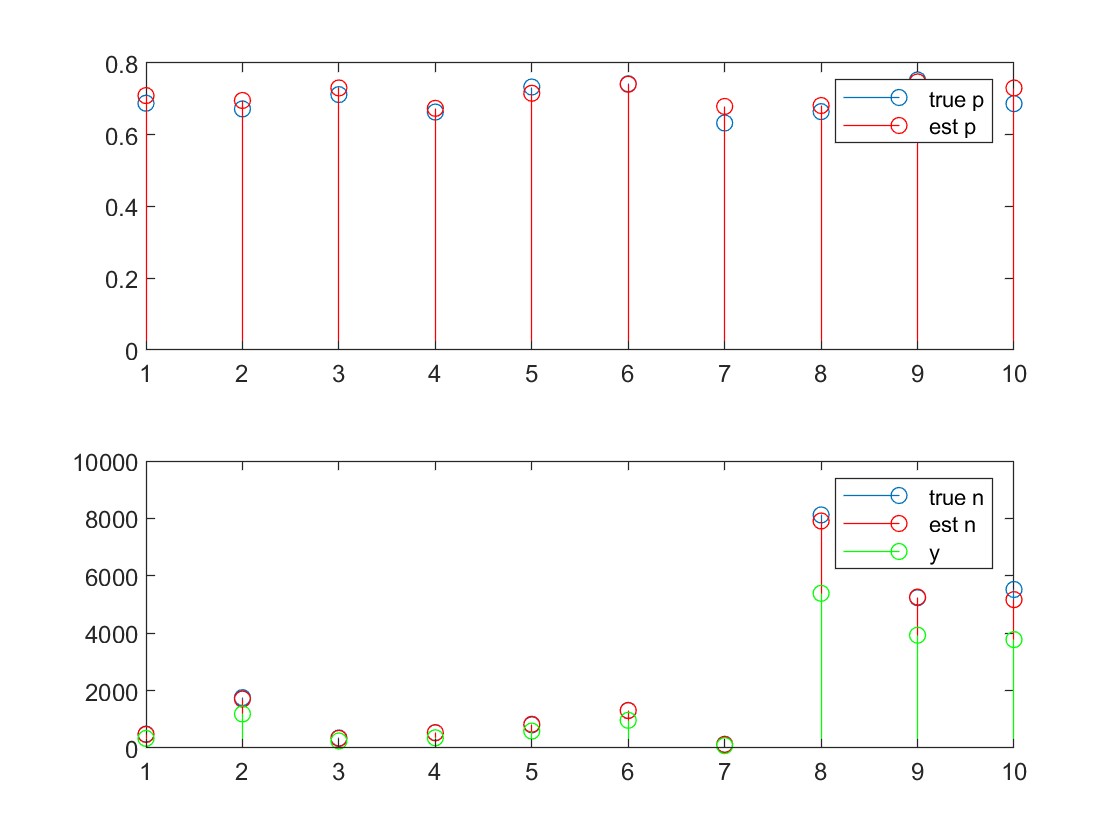
Fig. 1: The plot presents a comparison between the true value of $p$ and its estimated counterpart, as well as a comparison between the true value of $n$, the estimated value of $n$, and $y$. The relative $\ell_{1}$ error for $p$ stands at $0.035$, while the relative $\ell_{1}$ error for $n$ is $0.029$.

As demonstrated in Figure 1, the debiased solution generated by GRAUD is closely aligned with the ground truth, indicating high accuracy in our approach. The proximity of GRAUD’s output to the ground truth underscores its reliability in providing accurate results, thus justifying its application in this context.

5.2 Real Data Experiment

In the real-world experiment, we direct our attention towards emergency (911) call data originating from Atlanta, specifically from the year 2019, which comprises approximately 580,000 instances. It’s noteworthy that the actual number of emergency situations is likely higher than represented by these calls, as they tend to underestimate the true magnitude of emergencies. We make use of this data to establish the variable $y_{i}$ for every individual beat, with a beat referring to the distinct geographical area assigned to a police officer for patrolling. These beats subdivide Atlanta into 78 distinct sections, which offers a naturally discrete geographical division for our research.

To enhance our understanding, we create a graphical model in which each beat is symbolized as a node, and edges are formed between nodes that correspond to neighboring beats. This graph-based representation allows us to visualize and comprehend the spatial connections and proximity among the different beats in a more intuitive manner.

To supplement our dataset further, we include the census data from 2019, factoring in aspects such as population size, income, and level of education (quantified as the fraction of the population that has achieved at least a high school diploma). These factors constitute our $x_{ij}$ variables, thereby incorporating socioeconomic factors into our analysis.

To begin our analysis, we set the initial $p_{i}$ vector as a vector of all 0.8s and $n_{i}=y_{i}/p_{i}$. The localized solution we achieve from this starting point is represented in Figure 3. The yellow areas represent a higher discovery probability, and those areas with higher discovery rates are mainly located in the downtown, midtown or other prosperous areas in Atlanta. This makes sense because those flourishing areas usually have better public security and thus resulting in higher discovery rates.

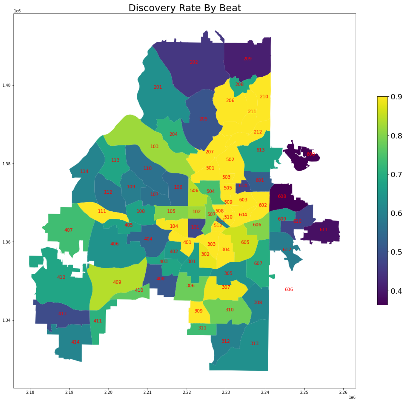
Fig. 2: The estimated $p_{i}$ in each beat when initializing with the discovery probability of all 0.8.

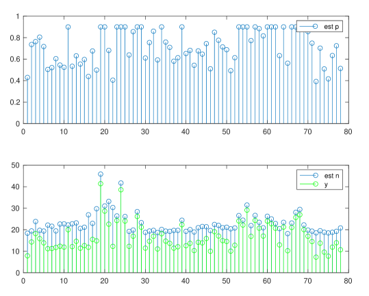
Fig. 3: The estimated $\hat{p}_{i}$ from data (when converges to locally). The $p_{i}$ are intialized to be constant 0.1. Clearly, the different regions may have different level of crime discovery.

6 Conclusion

In this paper, we proposed a novel graph prediction method for debiasing under-count data. We utilize the intrinsic graph structure in the problem and overcome the identifiability issue. We reformulate the problem as an optimization problem and establish the connection between the binomial n problem and the graph signal separation problem. We provide an alternating minimization optimization algorithm for efficiently recovering data. We establish recovery bounds and convergence results for our proposed method and conduct several experiments on both synthetic data and real data, demonstrating the accuracy and efficiency of our proposed method.

Acknowledgement

We would like to thank Sarah Huestis for her help with the real data experiment. This work is partially supported by an NSF CAREER CCF-1650913, and NSF DMS-2134037, CMMI-2015787, CMMI-2112533, DMS-1938106, and DMS-1830210, and a Coca-Cola Foundation fund.

Appendix

6.1 Proof of Lemma 7.1

Lemma 6.1.

If $X\sim\operatorname{Binomial}(n,p)$, then

$$\mathbb{P}\left(|X-np|\geq n^{1/2+\epsilon}\right)\leq 2e^{-n^{2\epsilon}/3p}$$

for small enough $\epsilon$.

We first introduce the following Chernoff Bound:

Lemma 6.2.

(Chernoff bound) Let $X\sim\operatorname{Binomial}(n,p)$ and let $\mu=\mathbb{E}[X]$. For any $0<\delta<1$ : Upper tail bound:

$$\mathbb{P}(X\geq(1+\delta)\mu)\leq\exp\left(-\frac{\delta^{2}\mu}{3}\right).$$

Lower tail bound:

$$\mathbb{P}(X\leq(1-\delta)\mu)\leq\exp\left(-\frac{\delta^{2}\mu}{2}\right),$$

where $\exp(x)=e^{x}$.

From Lemma 6.2, we have

$$\mathbb{P}(X\geq np+n^{1/2+\epsilon}) =\mathbb{P}(X\geq np(1+n^{-1/2+\epsilon}p^{-1}))$$ (9)

$$\leq\exp(-\frac{n^{-1}p^{-2}n^{2\epsilon}np}{3}$$

$$=\exp(-\frac{n^{2\epsilon}}{3p})$$

Similarly, we have the lower tail bound:

$$\mathbb{P}(X\leq np-n^{1/2+\epsilon})\leq\exp(-\frac{n^{2\epsilon}}{2p})$$ (10)

Combining the two inequalities, we have

$$\mathbb{P}\left(|X-np|\geq n^{1/2+\epsilon}\right)= \mathbb{P}(X\geq np+n^{1/2+\epsilon})+$$ (11)

$$\mathbb{P}(X\leq np-n^{1/2+\epsilon})$$

$$\leq \exp(-\frac{n^{2\epsilon}}{3p})+\exp(-\frac{n^{2\epsilon}}{2p})$$

$$\leq 2\exp(-\frac{n^{2\epsilon}}{3p})$$

6.2 Proof of Proposition 4.1

First, we show that the objective function is convex. Let $L(u,v)$ be the loss function, we have

$$\frac{\partial L}{\partial u}=2(u+v-\tilde{y}+\lambda_{2}Hu),$$ (12)

and

$$\frac{\partial L}{\partial v}=2(u+v-\tilde{y}+\lambda_{1}Lv).$$ (13)

We can compute the Hessian matrix $\tilde{H}$:

$$\left[\begin{array}[]{c c}I+\lambda_{2}H&I\\ I&I+\lambda_{1}L\end{array}\right]$$ (14)

For any $x=(u,v)^{T}$, we have

$$x^{T}\tilde{H}x =u^{T}(I+\lambda_{2}H)u+2u^{T}v+v^{T}(I+\lambda_{1}L)v$$ (15)

$$=\|u+v\|^{2}+\lambda_{2}u^{T}Hu+\lambda_{1}v^{T}LV\geq 0$$

This means $\tilde{H}$ is positive semidefinite, which leads to the convexity of the problem.

Then we prove the uniqueness of the solution. Suppose there are two different solutions $x=(u,v)$ and $x^{*}=(u^{*},v^{*})$. This means the gradient is zero at those two points, and we can derive

$$\lambda_{1}Lv =\lambda_{2}Hu=\tilde{y}-u-v$$ (16)

$$\lambda_{1}Lv^{*} =\lambda_{2}Hu^{*}=\tilde{y}-u^{*}-v^{*}$$

Define $\delta_{v}^{*}=v-v^{*}$, $\delta_{u}^{*}=u-u^{*}$, then

$$\lambda_{1}L\delta_{v} =\lambda_{2}H\delta_{u}=0-\delta_{u}-\delta_{v}$$ (17)

We can rewrite the equation into a quadratic optimization problem:

$$\min_{\delta_{v},\delta_{u}}\ \ f(\delta_{v},\delta_{u})=\|\delta_{v}+\delta_{u}\|^{2}+\lambda_{1}\delta_{v}^{T}L\delta_{v}+\lambda_{2}\delta_{u}^{T}H\delta_{u}.$$ (18)

$\delta_{v}^{*}$ and $\delta_{u}^{*}$ is a non-zero solution of this problem. We notice that $0$ is a solution of the problem and the minimum should be $0$. This means $f(\delta_{v}^{*},\delta_{u}^{*})=0$. Considering the non-negativity of each term, we have $\|\delta_{v}^{*}+\delta_{u}^{*}\|=0$, $\delta_{v}^{*T}L\delta_{v}^{*}=0$ and $\delta_{u}^{*T}H\delta_{u}^{*}=0$. This means $\delta_{v}^{*}$ is in the null space of $L$ and $\delta_{u}^{*}$ is in the null space of $H$. According to Assumption (2), the intersection of two null spaces is $0$, which means $\delta_{v}^{*}=\delta_{u}^{*}=0$. So the solution is unique.

6.3 Proof of Theorem 4.2

Suppose $\tilde{y}=n_{0}+p_{0}+\epsilon_{y}$, $v_{0}=\vec{h}+\epsilon_{u}$, and $u_{0}=X\beta_{0}+\epsilon_{v}$. Here the subscript $0$ means the ground truth, and $\vec{h}$ is the closest vector to $p_{0}$ in the null space of $L$.

From the assumption (1), we know that $\epsilon_{u}$ and $\epsilon_{v}$ are small and we can treat them as a kind of ”noise”. Denote $u-u_{0}=d_{u}$, $v-v_{0}=d_{v}$, then we can rewrite the original objective function (7):

$$\|\tilde{y}-u-v\|^{2}+\lambda_{1}v^{T}Lv+\lambda_{2}u^{T}Hu$$ (19)

$$=\|n_{0}+p_{0}+\epsilon_{y}-(d_{u}+u_{0})-(d_{v}+v_{0})\|^{2}+$$

$$\lambda_{1}(d_{v}+\vec{h}+\epsilon_{u})^{T}L(d_{v}+\vec{h}+\epsilon_{u})+$$

$$\lambda_{2}(d_{u}+X\beta_{0}+\epsilon_{v})^{T}H(d_{u}+X\beta_{0}+\epsilon_{v})$$

$$=\|\epsilon_{y}-d_{u}-d_{v}\|^{2}+\lambda_{1}(d_{v}+\epsilon_{u})^{T}L(d_{v}+\epsilon_{u})$$

$$+\lambda_{2}(d_{u}+\epsilon_{v})^{T}H(d_{u}+\epsilon_{v})$$

If we define $\tilde{d}_{v}=d_{v}+\epsilon_{u}$, $\tilde{d}_{u}=d_{u}+\epsilon_{v}$ and $\epsilon=\epsilon_{y}+\epsilon_{u}+\epsilon_{v}$, then the previous optimization problem is equivalent to

$$\min_{\tilde{d}_{v},\tilde{d}_{u}}L(\tilde{d}_{v},\tilde{d}_{u})=\|\epsilon-\tilde{d}_{v}-\tilde{d}_{u}\|^{2}+\lambda_{1}\tilde{d}_{v}^{T}L\tilde{d}_{v}+\lambda_{2}\tilde{d}_{u}^{T}H\tilde{d}_{u}$$ (20)

Let $\tilde{d}_{v}=\tilde{d}_{u}=0$, the objective function $L(\tilde{d}_{v},\tilde{d}_{u})=\|\epsilon\|^{2}$. This means that $L(\tilde{d}_{v}^{*},\tilde{d}_{u}^{*})\leq\|\epsilon\|^{2}$. Consequently, we have

$$\tilde{d}_{v}^{T}L\tilde{d}_{v}\leq\|\epsilon\|^{2}/\lambda_{1}$$ (21)

$$\tilde{d}_{u}^{T}H\tilde{d}_{u}\leq\|\epsilon\|^{2}/\lambda_{2}$$

Define $\sigma_{L}$ as the smallest positive singular value of matrix $L$, and $\sigma_{H}$ as the smallest positive singular value of matrix $H$. We can divide $\tilde{d}_{v}=\tilde{d}_{v\parallel}+\tilde{d}_{v\perp}$ and $\tilde{d}_{u}=\tilde{d}_{u\parallel}+\tilde{d}_{u\perp}$. Here $\tilde{d}_{v\parallel}$ is in the null space of $L$, $\tilde{d}_{v\perp}$ is orthogonal to the null space of $L$, $\tilde{d}_{u\parallel}$ is in the null space of $H$ and $\tilde{d}_{u\perp}$ is orthogonal to the null space of $H$, We have

$$\tilde{d}_{v}^{T}L\tilde{d}_{v}\geq\sigma_{L}\|d_{v\perp}\|^{2}$$ (22)

$$\tilde{d}_{u}^{T}H\tilde{d}_{u}\geq\sigma_{H}\|d_{u\perp}\|^{2}$$

Combining (21) and (22), we have $\|\tilde{d}_{v\perp}\|^{2}\leq\frac{\|\epsilon\|^{2}}{\lambda_{1}\sigma_{L}}$ and $\|\tilde{d}_{u\perp}\|^{2}\leq\frac{\|\epsilon\|^{2}}{\lambda_{2}\sigma_{H}}$. Next we would like to bound $\|\tilde{d}_{v\parallel}\|$ and $\|\tilde{d}_{u\parallel}\|$. Since $\tilde{d}_{v\parallel}$ is in the column space of $X$, there exists $a_{1},a_{2},\cdots,a_{r_{X}}$ s.t. $\tilde{d}_{v\parallel}=\sum_{i=1}^{r_{X}}a_{i}x_{i}$, where $x_{1},\cdots,x_{r_{X}}$ be the basis of the column space of $X$. Similarly, there exists $b_{1},b_{2},\cdots,b_{r_{L}}$ s.t. $\tilde{d}_{u\parallel}=\sum_{i=1}^{r_{L}}b_{i}l_{i}$, where $l_{1},\cdots,l_{r_{L}}$ be the basis of the null space of $L$. It is obvious that $\|\tilde{d}_{v\parallel}\|^{2}=\sum_{i=1}^{r_{X}}a_{i}^{2}$ and $\|\tilde{d}_{u\parallel}\|^{2}=\sum_{i=1}^{r_{L}}b_{i}^{2}$. From Assumption (2), we have

$$\|\tilde{d}_{v\parallel}+\tilde{d}_{u\parallel}\|^{2} \geq\delta_{1}(\|\sum_{i=1}^{r_{X}}a_{i}^{2}+\sum_{i=1}^{r_{L}}b_{i}^{2})$$ (23)

$$=\delta_{1}(\|\tilde{d}_{v\parallel}\|^{2}+\|\tilde{d}_{u\parallel}\|^{2})$$

Since $L(\tilde{d}_{v}^{*},\tilde{d}_{u}^{*})\leq\|\epsilon\|^{2}$, we also have $\|\epsilon-\tilde{d}_{v}-\tilde{d}_{u}\|\leq\|\epsilon\|$. Meanwhile,

$$\|\epsilon\| \geq\|\epsilon-\tilde{d}_{v}-\tilde{d}_{u}\|=\|\epsilon-(\tilde{d}_{v\parallel}+\tilde{d}_{v\perp})-(\tilde{d}_{u\parallel}+\tilde{d}_{u\perp})\|$$ (24)

$$\geq\|\tilde{d}_{v\parallel}+\tilde{d}_{u\parallel}\|-\|\epsilon\|-\|\tilde{d}_{v\perp}\|-\|\tilde{d}_{u\perp}\|$$

$$\geq\delta_{1}^{1/2}(\|\tilde{d}_{v\parallel}\|^{2}+\|\tilde{d}_{u\parallel}\|^{2})^{1/2}-\|\epsilon\|-\frac{\|\epsilon\|}{\sqrt{\lambda_{1}\sigma_{L}}}-\frac{\|\epsilon\|}{\sqrt{\lambda_{2}\sigma_{H}}}$$

This means

$$\delta_{1}^{1/2}(\|\tilde{d}_{v\parallel}\|^{2}+\|\tilde{d}_{u\parallel}\|^{2})^{1/2}\leq\|\epsilon\|(2+\frac{1}{\sqrt{\lambda_{1}\sigma_{L}}}+\frac{1}{\sqrt{\lambda_{2}\sigma_{H}}})$$ (25)

Define $c_{0}=2+\frac{1}{\sqrt{\lambda_{1}\sigma_{L}}}+\frac{1}{\sqrt{\lambda_{2}\sigma_{H}}}$, we have

$$\|\tilde{d}_{v\parallel}\|^{2}+\|\tilde{d}_{u\parallel}\|^{2}\leq\frac{c_{0}^{2}\|\epsilon\|^{2}}{\delta_{1}}$$ (26)

As a result, we can derive that

$$\|\tilde{d}_{v}\|^{2} =\|\tilde{d}_{v\parallel}\|^{2}+\|\tilde{d}_{v\perp}\|^{2}$$ (27)

$$\leq\|\epsilon\|^{2}(\frac{c_{0}^{2}}{\delta_{1}}+\frac{1}{\lambda_{1}\sigma_{L}})$$

$$\|\tilde{d}_{u}\|^{2} =\|\tilde{d}_{u\parallel}\|^{2}+\|\tilde{d}_{u\perp}\|^{2}$$

$$\leq\|\epsilon\|^{2}(\frac{c_{0}^{2}}{\delta_{1}}+\frac{1}{\lambda_{2}\sigma_{H}})$$

Considering that $\tilde{d}_{v}=d_{v}+\epsilon_{u}$ and $\tilde{d}_{u}=d_{u}+\epsilon_{y}$, we can finally get a bound on the error $d_{v}$ and $d_{u}$:

$$\|d_{v}\|^{2} \leq\|\tilde{d}_{v}\|^{2}+\|\epsilon_{u}\|^{2}$$ (28)

$$\leq\|\epsilon\|^{2}(\frac{c_{0}^{2}}{\delta_{1}}+\frac{1}{\lambda_{2}\sigma_{H}})+\|\epsilon_{u}\|^{2}$$

$$=\tilde{c_{1}}\|\epsilon\|^{2}+\|\epsilon_{u}\|^{2}$$

$$\|d_{u}\|^{2} \leq\|\tilde{d}_{u}\|^{2}+\|\epsilon_{v}\|^{2}$$

$$\leq\|\epsilon\|^{2}(\frac{c_{0}^{2}}{\delta_{1}}+\frac{1}{\lambda_{1}\sigma_{L}})+\|\epsilon_{v}\|^{2}$$

$$=\tilde{c_{2}}\|\epsilon\|^{2}+\|\epsilon_{v}\|^{2}$$

References

- [1] Lorna Hazell and Saad AW Shakir, “Under-reporting of adverse drug reactions,” Drug safety, vol. 29, no. 5, pp. 385–396, 2006.
- [2] Angela Watson, Barry Watson, and Kirsten Vallmuur, “Estimating under-reporting of road crash injuries to police using multiple linked data collections,” Accident Analysis & Prevention, vol. 83, pp. 18–25, 2015.
- [3] Junaid Shuja, Eisa Alanazi, Waleed Alasmary, and Abdulaziz Alashaikh, “Covid-19 open source data sets: a comprehensive survey,” Applied Intelligence, vol. 51, pp. 1296–1325, 2021.
- [4] A DasGupta and Herman Rubin, “Estimation of binomial parameters when both n, p are unknown,” Journal of Statistical Planning and Inference, vol. 130, no. 1-2, pp. 391–404, 2005.
- [5] Sanjib Basu, “Ch. 31. bayesian inference for the number of undetected errors,” Handbook of Statistics, vol. 22, pp. 1131–1150, 2003.
- [6] Sanjib Basu and Nader Ebrahimi, “Bayesian capture-recapture methods for error detection and estimation of population size: Heterogeneity and dependence,” Biometrika, vol. 88, no. 1, pp. 269–279, 2001.
- [7] Norman Draper and Irwin Guttman, “Bayesian estimation of the binomial parameter,” Technometrics, vol. 13, no. 3, pp. 667–673, 1971.
- [8] Dorian Feldman and Martin Fox, “Estimation of the parameter n in the binomial distribution,” Journal of the American Statistical Association, vol. 63, no. 321, pp. 150–158, 1968.
- [9] Adrian E Raftery, “Inference for the binomial n parameter: A bayes empirical bayes approach. revision.,” Tech. Rep., WASHINGTON UNIV SEATTLE DEPT OF STATISTICS, 1987.
- [10] Lucy Whitaker, “On the poisson law of small numbers,” Biometrika, vol. 10, no. 1, pp. 36–71, 1914.
- [11] P Fisher et al., “Negative binomial distribution.,” Annals of Eugenics, vol. 11, pp. 182–787, 1941.
- [12] John Burdon Sanderson Haldane, “The fitting of binomial distributions,” Annals of Eugenics, vol. 11, no. 1, pp. 179–181, 1941.
- [13] William D Kahn, “A cautionary note for bayesian estimation of the binomial parameter n,” The American Statistician, vol. 41, no. 1, pp. 38–40, 1987.
- [14] GG Hamedani and GG Walter, “Bayes estimation of the binomial parameter n,” Communications in Statistics-Theory and Methods, vol. 17, no. 6, pp. 1829–1843, 1988.
- [15] Erdogan Günel and Daniel Chilko, “Estimation of parameter n of the binomial distribution,” Communications in Statistics-Simulation and Computation, vol. 18, no. 2, pp. 537–551, 1989.
- [16] Shixiang Zhu and Yao Xie, “Generalized hypercube queuing models with overlapping service regions,” arXiv preprint arXiv:2304.02824, 2023.
- [17] David I Shuman, Sunil K Narang, Pascal Frossard, Antonio Ortega, and Pierre Vandergheynst, “The emerging field of signal processing on graphs: Extending high-dimensional data analysis to networks and other irregular domains,” IEEE signal processing magazine, vol. 30, no. 3, pp. 83–98, 2013.
- [18] Alexander Von Eye, Eun-Young Mun, and Patrick Mair, “Log-linear modeling,” Wiley Interdisciplinary Reviews: Computational Statistics, vol. 4, no. 2, pp. 218–223, 2012.
- [19] FENG Changyong, WANG Hongyue, LU Naiji, CHEN Tian, HE Hua, LU Ying, et al., “Log-transformation and its implications for data analysis,” Shanghai archives of psychiatry, vol. 26, no. 2, pp. 105, 2014.