Preconditioning techniques for generalized Sylvester matrix equations

Abstract

Sylvester matrix equations are ubiquitous in scientific computing. However, few solution techniques exist for their generalized multiterm version, as they recently arose in stochastic Galerkin finite element discretizations and isogeometric analysis. In this work, we consider preconditioning techniques for the iterative solution of generalized Sylvester equations. They consist in constructing low Kronecker rank approximations of either the operator itself or its inverse. In the first case, applying the preconditioning operator requires solving standard Sylvester equations, for which very efficient solution methods have already been proposed. In the second case, applying the preconditioning operator only requires computing matrix-matrix multiplications, which are also highly optimized on modern computer architectures. Moreover, low Kronecker rank approximate inverses can be easily combined with sparse approximate inverse techniques, thereby further speeding up their application with little or no damage to their preconditioning capability.

Keywords: Generalized Sylvester equations, Low Kronecker rank, Nearest Kronecker product, Alternating least squares, Sparse approximate inverse, Isogeometric analysis. 2020 MSC: 65F08, 65F45, 65F50.

1 Introduction

We consider the numerical solution of generalized Sylvester matrix equations

$$\sum_{k=1}^{r}B_{k}XA_{k}^{T}=C$$ (1.1)

where $A_{k}\in\mathbb{R}^{n\times n}$, $B_{k}\in\mathbb{R}^{m\times m}$ for all $k=1,\dots,r$ and $X,C\in\mathbb{R}^{m\times n}$. Generalized Sylvester equations are at the forefront of many applications in scientific computing. Some important special cases have attracted considerable interest and are listed below.

• The generalized Sylvester equation (for $r=1$)

  $$B_{1}XA_{1}^{T}=C$$ (1.2)

  is its simplest instance. It appears in explicit time integration schemes for tensorized finite element discretizations of certain time dependent partial differential equations (PDEs) in two spatial dimensions [1, 2, 3]. If $A_{1}$ and $B_{1}$ are invertible, the solution of (1.2) is particularly simple since $X=B_{1}^{-1}CA_{1}^{-T}$ only requires solving $n$ linear systems with $B_{1}$ and $m$ linear systems with $A_{1}$. If $A_{1}=I_{n}$, (1.2) reduces to a standard linear system with multiple right-hand sides.

• The generalized Sylvester equation (for $r=2$)

  $$B_{1}XA_{1}^{T}+B_{2}XA_{2}^{T}=C$$ (1.3)

  stems, for instance, from tensorized finite element discretizations of certain differential operators on structured domains in two spatial dimensions [4, 5] and generalized eigenproblems [6]. Some special cases of (1.3) are:

  • The (standard) Sylvester equation (obtained for $A_{1}=I_{n}$ and $B_{2}=I_{m}$), which appears in various applications, including block-diagonalization of block triangular matrices [7, 8], finite difference discretizations of certain PDEs [9, 10], and eigenvalue problems [8, 11]. Sylvester equations are also the main building block for iteratively solving more complicated nonlinear matrix equations, as they arise for computing invariant subspaces [8]. Although (1.3) may sometimes be transformed to a standard Sylvester equation, this transformation is neither always possible nor desirable if the coefficient matrices are ill-conditioned.

  • The Lyapunov equation (obtained for $A_{2}=B_{1}$ and $A_{1}=B_{2}=I_{n}$), which is itself a particular case of the (standard) Sylvester equation and arises, for instance, in the stability analysis of dynamical systems [12] and control theory [13].

  • The Stein equation (obtained for $A_{1}=I_{n}$ and $B_{1}=I_{m}$), also known as the discrete-time Sylvester equation, appears in the analysis of dynamical systems [14] and in the stage equations of implicit Runge-Kutta methods [15].

Solution techniques for generalized Sylvester equations most critically depend on the number of terms $r$ of the equation. While the case $r=1$ is straightforward, the case $r=2$ is already significantly more challenging and an impressive collection of methods have been proposed. Efficient solvers exploit the structure of the equation and its solution, including the sparsity and relative size of the coefficient matrices [16]. Since the pioneering work of Bartels and Stewart [17], many different solution techniques have emerged including alternating direction implicit (ADI) iteration [18], recursive blocked algorithms [19], low-rank and sparse data formats [20] and tensorized Krylov subspace methods [10] to name just a few. An exhaustive list of methods is beyond the scope of this article and we instead refer to [16] and the references therein for an overview.

While the special matrix equations listed above account for a vast number of publications, the more general equation (1.1) has received much less attention. The practical utility of these equations may simply explain the difference: while numerous applications have driven the development of solution techniques for (standard) Sylvester and Lyapunov equations, the generalized Sylvester equation (1.1) was far less common and has mainly been considered of theoretical interest [16, 7]. However, the gap is quickly being filled as recent developments in stochastic Galerkin finite element methods [21, 22] and isogeometric analysis [23] now lead to solving generalized Sylvester equations with $r>2$.

Unfortunately, the vast majority of the solution techniques proposed for $r=2$ are not applicable to $r>2$. The main reason is that solution techniques for $r=2$ rely on results for joint diagonalization (or triangularization) of matrix pairs such as generalized eigendecompositions (or Schur decompositions), which are also the basis for existence and uniqueness results [24]. These techniques generally do not extend to sequences of matrices $\{A_{k}\}_{k=1}^{r}$ and $\{B_{k}\}_{k=1}^{r}$ (with $r>2$), unless the elements of these sequences are related in some special way (e.g. they are powers of one same matrix [25] or are a commuting family of symmetric matrices). Therefore, most solution techniques for (1.1) have instead focused on solving the equivalent linear system [26, Lemma 4.3.1]

$$\left(\sum_{k=1}^{r}A_{k}\otimes B_{k}\right)\mathbf{x}=\mathbf{c}.$$ (1.4)

with $\mathbf{x}=\operatorname{\operatorname{vec}}(X)$ and $\mathbf{c}=\operatorname{\operatorname{vec}}(C)$. We recall that the vectorization of a matrix $A$, denoted $\operatorname{\operatorname{vec}}(A)$, stacks the columns of $A$ on top of each other. The transformation to (1.4) shows that solving the generalized Sylvester equation (1.1) is equivalent to solving a special linear system where the coefficient matrix is the sum of $r$ Kronecker products. Such a matrix is said to have Kronecker rank $r$ if $r$ is the smallest number of terms in the sum. In this article, we will focus on the iterative solution of (1.4) as a way of solving generalized Sylvester equations.

The rest of the article is structured as follows: In Section 2 we first recall some iterative solution techniques applicable to linear matrix equations. Similarly to iterative methods for linear systems, these methods may converge very slowly when the associated system matrix is ill-conditioned, creating a formidable strain on memory resources. Therefore, in Sections 3 and 4, we exploit the underlying Kronecker structure of the system matrix to design efficient and robust preconditioning strategies. These strategies aim at finding low Kronecker rank approximations of the operator itself (Section 3) or its inverse (Section 4). Furthermore, if the inverse admits a good sparse approximation, we propose to combine our strategies with sparse approximate inverse techniques to construct low Kronecker rank sparse approximate inverses. Section 5 gathers a few numerical experiments illustrating the effectiveness of our preconditioning strategies for solving generalized Sylvester equations stemming from isogeometric analysis, a tensorized finite element method. Finally, conclusions are drawn in Section 6.

2 Iterative solution techniques for matrix equations

Since direct solution methods are generally not applicable to (1.1), we investigate its iterative solution. For this purpose, we denote $\mathcal{M}\colon\mathbb{R}^{m\times n}\to\mathbb{R}^{m\times n}$ the linear operator defined as

$$\mathcal{M}(X)=\sum_{k=1}^{r}B_{k}XA_{k}^{T}.$$ (2.1)

This operator has a Kronecker structured matrix representation given by

$$M=\sum_{k=1}^{r}A_{k}\otimes B_{k}.$$ (2.2)

We will generally use curly letters for linear operators and straight letters for their associated matrix.

Since (1.1) and (1.4) represent the same set of equations but written differently, iterative solution techniques for solving (1.1) are specialized versions of well-known iterative methods for solving linear systems. The global GMRES (Gl-GMRES) method is one of them. Originally proposed for solving linear systems with multiple right-hand sides, the method found natural applications for solving linear matrix equations [27]. As a matter of fact, the idea was already laid out in [28] several years earlier. As the name suggests, the Gl-GMRES method is an adaptation of the famous GMRES method [29] for linear systems whose coefficient matrix is expressed as a sum of Kronecker products. It exploits the fact that

$$Y=\mathcal{M}(X)\iff\mathbf{y}=M\mathbf{x}$$ (2.3)

with $\mathbf{x}=\operatorname{\operatorname{vec}}(X)$, $\mathbf{y}=\operatorname{\operatorname{vec}}(Y)$ together with $\mathcal{M}$ and $M$ defined in (2.1) and (2.2), respectively. Instead of vector Krylov subspaces, the Gl-GMRES method builds the matrix Krylov subspace [30]

$$\mathcal{K}_{k}(\mathcal{M},V)=\operatorname{\operatorname{span}}(V,\mathcal{M}(V),\dots,\mathcal{M}^{k-1}(V))$$

where $V\in\mathbb{R}^{m\times n}$ and $\mathcal{M}^{i}(V)$ is defined recursively as $\mathcal{M}^{i}(V)=\mathcal{M}(\mathcal{M}^{i-1}(V))$. In a standard GMRES method, fast matrix-vector multiplications with $M=\sum_{k=1}^{r}A_{k}\otimes B_{k}$ would evidently also use the connection (2.3). However, the Gl-GMRES method works with matrices all along the process and avoids repeatedly reshaping vectors to matrices and back. Therefore, it is well-suited for iteratively solving the generalized Sylvester equation (1.1). Clearly, other Krylov subspace methods such as the conjugate gradient method (CG) [31, 32] and the biconjugate gradient stabilized method (Bi-CGSTAB) [33] can also be adapted for solving linear matrix equations.

However, since Gl-GMRES is mathematically equivalent to GMRES, any ill-conditioning of $M$ impedes on its convergence. Preconditioning techniques are commonly employed for speeding up the convergence of iterative methods. In the context of matrix equations, they take the form of a preconditioning operator $\mathcal{P}\colon\mathbb{R}^{m\times n}\to\mathbb{R}^{m\times n}$. Preconditioning can be straightforwardly incorporated in the Gl-GMRES method by adapting preconditioned versions of the standard GMRES method [32]. Algorithm 1, for instance, presents the right preconditioned variant of the Gl-GMRES method. Preconditioning techniques for Sylvester and Lyapunov equations were already considered in [30, 28] but cannot be extended to $r>2$ since they rely on the special structure of the equation.

1:Input: Linear operator $\mathcal{M}\colon\mathbb{R}^{m\times n}\to\mathbb{R}^{m\times n}$, preconditioning operator $\mathcal{P}\colon\mathbb{R}^{m\times n}\to\mathbb{R}^{m\times n}$, right-hand side matrix $C\in\mathbb{R}^{m\times n}$, starting matrix $X_{0}\in\mathbb{R}^{m\times n}$

2:Output: Approximate solution $X_{k}$ to $\mathcal{M}(X)=C$

3:

4:Set $R_{0}=C-\mathcal{M}(X_{0})$

5:Set $\beta_{0}=\|R_{0}\|_{F}$, $U_{1}=R_{0}/\beta_{0}$

6:for $j=1,2,\dots,k$ do

7:     Compute $W=\mathcal{M}(\mathcal{P}(U_{j}))$

8:     for $i=1,\dots,j$ do

9:         Compute $h_{ij}=\langle U_{i},W\rangle_{F}$

10:         Compute $W=W-h_{ij}U_{i}$

11:     end for

12:     Set $h_{j+1,j}=\|W\|_{F}$

13:     Set $U_{j+1}=W/h_{j+1,j}$

14:     Find $\mathbf{y}_{j}=\operatorname{argmin}_{\mathbf{y}\in\mathbb{R}^{j}}\|\beta_{0}\mathbf{e}_{1}-\tilde{H}_{j}\mathbf{y}\|_{2}$ $\triangleright$ $\tilde{H}_{j}\in\mathbb{R}^{j+1\times j}$

15:     Set $\beta_{j}=\|\beta_{0}\mathbf{e}_{1}-\tilde{H}_{j}\mathbf{y}_{j}\|_{2}$ $\triangleright$ $\beta_{j}=\|C-\mathcal{M}(X_{j})\|_{F}$

16:end for

17:Return $X_{k}=X_{0}+\mathcal{P}(\sum_{j=1}^{k}y_{j}U_{j})$ $\triangleright$ $\mathbf{y}_{k}^{T}=(y_{1},\dots,y_{k})$

Algorithm 1 Right preconditioned Gl-GMRES

If the number of iterations $k$ remains relatively small, applying the operators $\mathcal{M}$ and $\mathcal{P}$ in line 4 is the most expensive step in Algorithm 1. Assuming that all factor matrices $A_{k}$ and $B_{k}$ are dense for $k=1,\dots,r$, storing them requires $O(r(n^{2}+m^{2}))$ while applying $\mathcal{M}(X)$ requires $O(r(n^{2}m+nm^{2}))$ operations. In comparison, when $M$ is formed explicitly, matrix-vector multiplications require $O(n^{2}m^{2})$ operations, in addition to the prohibitive storage requirements amounting to $O(n^{2}m^{2})$. The cost of applying the preconditioning operator will depend on its definition and this will be the focus of the next few sections.

3 Nearest Kronecker product preconditioner

In Section 1, we had noted that the solution of a generalized Sylvester equation can be computed (relatively) easily when $r\leq 2$. Indeed, for $r=2$ the equation may often be reformulated as a standard Sylvester equation for which there exists dedicated solvers while for $r=1$ the equation reduces to a very simple matrix equation, which can be solved straightforwardly. Therefore, a first preconditioning strategy could rely on finding the best Kronecker rank $1$ or $2$ approximation of $M=\sum_{k=1}^{r}A_{k}\otimes B_{k}$ and use it as a preconditioning operator. Kronecker rank $1$ preconditioners have already been proposed for many different applications including image processing [34], Markov chains [35, 36, 37], stochastic Galerkin [22] and tensorized [1, 2, 38] finite element methods. Extensions to Kronecker rank $2$ preconditioners have been considered in [5, 4] but not for preconditioning generalized Sylvester equations. The problem of finding the best Kronecker product approximation of a matrix (not necessarily expressed as a sum of Kronecker products) was first investigated by Van Loan and Pitsianis [39]. A more modern presentation followed in [40]. We adopt the same general framework for the time being and later specialize it to our problem. For the best Kronecker rank 1 approximation of a matrix $M\in\mathbb{R}^{nm\times nm}$, factor matrices $Y\in\mathbb{R}^{n\times n}$ and $Z\in\mathbb{R}^{m\times m}$ are sought such that $\phi_{M}(Y,Z)=\|M-Y\otimes Z\|_{F}$ is minimized. Van Loan and Pitsianis observed that both the Kronecker product $Y\otimes Z$ and $\operatorname{\operatorname{vec}}(Y)\operatorname{\operatorname{vec}}(Z)^{T}$ form all the products $y_{ij}z_{kl}$ for $i,j=1,\dots,n$ and $k,l=1,\dots,m$ but at different locations. Thus, there exists a linear mapping $\mathcal{R}\colon\mathbb{R}^{nm\times nm}\to\mathbb{R}^{n^{2}\times m^{2}}$ (which they called rearrangement) such that $\mathcal{R}(Y\otimes Z)=\operatorname{\operatorname{vec}}(Y)\operatorname{\operatorname{vec}}(Z)^{T}$. This mapping is defined explicitly by considering a block matrix $A$ where $A_{ij}\in\mathbb{R}^{m\times m}$ for $i,j=1,\dots,n$. Then, by definition

$$A=\begin{pmatrix}A_{11}&\cdots&A_{1n}\\ \vdots&\ddots&\vdots\\ A_{n1}&\cdots&A_{nn}\end{pmatrix}\qquad\mathcal{R}(A)=\begin{pmatrix}\operatorname{\operatorname{vec}}(A_{11})^{T}\\ \operatorname{\operatorname{vec}}(A_{21})^{T}\\ \vdots\\ \operatorname{\operatorname{vec}}(A_{nn})^{T}\end{pmatrix}.$$

By construction, for a matrix $A=Y\otimes Z$,

$$Y\otimes Z=\begin{pmatrix}y_{11}Z&\cdots&y_{1n}Z\\ \vdots&\ddots&\vdots\\ y_{n1}Z&\cdots&y_{nn}Z\end{pmatrix}\qquad\mathcal{R}(Y\otimes Z)=\begin{pmatrix}y_{11}\operatorname{\operatorname{vec}}(Z)^{T}\\ y_{21}\operatorname{\operatorname{vec}}(Z)^{T}\\ \vdots\\ y_{nn}\operatorname{\operatorname{vec}}(Z)^{T}\end{pmatrix}=\operatorname{\operatorname{vec}}(Y)\operatorname{\operatorname{vec}}(Z)^{T}.$$

More generally, since the vectorization operator is linear,

$$\mathcal{R}\left(\sum_{s=1}^{r}Y_{s}\otimes Z_{s}\right)=\sum_{s=1}^{r}\operatorname{\operatorname{vec}}(Y_{s})\operatorname{\operatorname{vec}}(Z_{s})^{T}.$$

Therefore, $\mathcal{R}$ transforms a Kronecker rank $r$ matrix into a rank $r$ matrix. Since rearranging the entries of a matrix does not change its Frobenius norm, the minimization problem becomes

$$\min\phi_{M}(Y,Z)=\min\|M-Y\otimes Z\|_{F}=\min\|\mathcal{R}(M)-\mathcal{R}(Y\otimes Z)\|_{F}=\min\|\mathcal{R}(M)-\operatorname{\operatorname{vec}}(Y)\operatorname{\operatorname{vec}}(Z)^{T}\|_{F}.$$

Thus, finding the best factor matrices $Y$ and $Z$ is equivalent to finding the best rank 1 approximation of $\mathcal{R}(M)$. Moreover generally, finding the best factor matrices $Y_{s}$ and $Z_{s}$ for $s=1,\dots,q$ defining the best Kronecker rank $q$ approximation is equivalent to finding the best rank $q$ approximation of $\mathcal{R}(M)$, which can be conveniently done using a truncated singular value decomposition (SVD). These computations are particularly cheap in our context given that $\mathcal{R}(M)$ is already in low-rank format. Note that applying the inverse operator $\mathcal{R}^{-1}$ to the SVD of $\mathcal{R}(M)$ enables to express $M$ as

$$M=\sum_{k=1}^{r}\sigma_{k}(U_{k}\otimes V_{k})$$ (3.1)

where $U_{k}$ and $V_{k}$ are reshapings of the $k$th left and right singular vectors of $\mathcal{R}(M)$, respectively, and $\sigma_{k}$ are the singular values for $k=1,\dots,r$. The orthogonality of the left and right singular vectors ensures that $\langle U_{i},U_{j}\rangle_{F}=\delta_{ij}$, $\langle V_{j},V_{j}\rangle_{F}=\delta_{ij}$ and $\langle M,(U_{i}\otimes V_{i})\rangle_{F}=\sigma_{i}$, where $\langle.,.\rangle_{F}$ denotes the Frobenius inner product. The best Kronecker rank $q$ approximation $P$ then simply consists in retaining the first $q$ terms of the sum in (3.1) and the approximation error is then given by the tail of the singular values

$$\|M-P\|_{F}^{2}=\sum_{k=q+1}^{r}\sigma_{k}^{2}.$$ (3.2)

The procedure is summarized in Algorithm 1 and is referred to as the SVD approach. We emphasize that we only consider $q\leq 2$ for constructing a practical preconditioner. For $q=1$, the resulting preconditioner is commonly referred to as the nearest Kronecker product preconditioner (NKP) [35, 38]. We will abusively use the same terminology for $q=2$.

1:Input:

2:Factor matrices $\{A_{k}\}_{k=1}^{r}\subset\mathbb{R}^{n\times n}$ and $\{B_{k}\}_{k=1}^{r}\subset\mathbb{R}^{m\times m}$

3:Kronecker rank $q\leq r$

4:Output:

5:Factor matrices $Y_{s}$ and $Z_{s}$ for $s=1,\dots,q$ such that $\sum_{s=1}^{q}Y_{s}\otimes Z_{s}\approx\sum_{k=1}^{r}A_{k}\otimes B_{k}$

6:

7:Set $V_{A}=[\operatorname{\operatorname{vec}}(A_{1}),\dots,\operatorname{\operatorname{vec}}(A_{r})]$

8:Set $V_{B}=[\operatorname{\operatorname{vec}}(B_{1}),\dots,\operatorname{\operatorname{vec}}(B_{r})]$

9:Compute the thin QR factorization $V_{A}=Q_{A}R_{A}$

10:Compute the thin QR factorization $V_{B}=Q_{B}R_{B}$

11:Compute the SVD $R_{A}R_{B}^{T}=\tilde{U}\Sigma\tilde{V}^{T}$ $\triangleright$ $\Sigma=\operatorname{\operatorname{diag}}(\sigma_{1},\dots,\sigma_{r})$

12:Set $V_{Y}=Q_{A}\tilde{U}\Sigma^{1/2}$ $\triangleright$ $V_{Y}=[\operatorname{\operatorname{vec}}(Y_{1}),\dots,\operatorname{\operatorname{vec}}(Y_{r})]$

13:Set $V_{Z}=Q_{B}\tilde{V}\Sigma^{1/2}$ $\triangleright$ $V_{Z}=[\operatorname{\operatorname{vec}}(Z_{1}),\dots,\operatorname{\operatorname{vec}}(Z_{r})]$

14:Return and reshape the first $q$ columns of $V_{Y}$ and $V_{Z}$.

Algorithm 1 Best Kronecker rank $q$ approximation

The SVD approach to the best Kronecker product approximation in the Frobenius norm is well established in the numerical linear algebra community. However, Van Loan and Pitsianis also proposed an alternating least squares approach, which in our context might be cheaper. We both specialize their strategy to Kronecker rank $r$ matrices and extend it to Kronecker rank $q$ approximations. Adopting the same notations as in Algorithm 1 and employing the reordering $\mathcal{R}$, we obtain

$$\left\|\sum_{k=1}^{r}A_{k}\otimes B_{k}-\sum_{s=1}^{q}Y_{s}\otimes Z_{s}\right\|_{F}=\left\|\sum_{k=1}^{r}\operatorname{\operatorname{vec}}(A_{k})\operatorname{\operatorname{vec}}(B_{k})-\sum_{s=1}^{q}\operatorname{\operatorname{vec}}(Y_{s})\operatorname{\operatorname{vec}}(Z_{s})\right\|_{F}=\|V_{A}V_{B}^{T}-V_{Y}V_{Z}^{T}\|_{F}$$ (3.3)

If the (linearly independent) matrices $Z_{s}$ are fixed for $s=1,\dots,q$, the optimal solution of the least squares problem (3.3) is given by

$$V_{Y}=V_{A}V_{B}^{T}V_{Z}(V_{Z}^{T}V_{Z})^{-1}.$$ (3.4)

If instead all matrices $Y_{s}$ are fixed for $s=1,\dots,q$, the optimal solution of (3.3) is given by the similar looking expression

$$V_{Z}=V_{B}V_{A}^{T}V_{Y}(V_{Y}^{T}V_{Y})^{-1}.$$ (3.5)

Equations (3.4) and (3.5) reveal that all factor matrices $Y_{s}$ and $Z_{s}$ for $s=1,\dots,q$ are linear combinations of $A_{k}$ and $B_{k}$, respectively, which could already be inferred from the SVD approach. This finding was already stated in [39] and proved in [35, Theorem 4.1] for $q=1$ and [38, Theorem 4.2] for arbitrary $q$. In particular, for $q=1$, after some reshaping, equations (3.4) and (3.5) reduce to

$$Y=\sum_{k=1}^{r}\frac{\langle B_{k},Z\rangle_{F}}{\langle Z,Z\rangle_{F}}A_{k}\quad\text{and}\quad Z=\sum_{k=1}^{r}\frac{\langle A_{k},Y\rangle_{F}}{\langle Y,Y\rangle_{F}}B_{k},$$

respectively, which can also be deduced from [39, Theorem 4.1]. Our derivations are summarized in Algorithm 2. The norm of the residual is used as stopping criterion in the alternating least squares algorithm. It can be cheaply evaluated without forming the Kronecker products explicitly since

$$\|V_{A}V_{B}^{T}-V_{Y}V_{Z}^{T}\|_{F}^{2} =\|V_{A}V_{B}^{T}\|_{F}^{2}-2\langle V_{A}V_{B}^{T},V_{Y}V_{Z}^{T}\rangle_{F}+\|V_{Y}V_{Z}^{T}\|_{F}^{2}$$

$$=\langle V_{A}^{T}V_{A},V_{B}^{T}V_{B}\rangle_{F}-2\langle V_{A}^{T}V_{Y},V_{B}^{T}V_{Z}\rangle_{F}+\langle V_{Y}^{T}V_{Y},V_{Z}^{T}V_{Z}\rangle_{F}.$$

A more explicit expression already appeared in [35, Theorem 4.2] for $r=2$ and $q=1$. Our expression generalizes it to arbitrary $r$ and $q$.

1:Input:

2:Factor matrices $\{A_{k}\}_{k=1}^{r}\subset\mathbb{R}^{n\times n}$ and $\{B_{k}\}_{k=1}^{r}\subset\mathbb{R}^{m\times m}$

3:Linearly independent factor matrices $Z_{s}\in\mathbb{R}^{m\times m}$ for $s=1,\dots,q$

4:Tolerance $\epsilon>0$ and maximum number of iterations $N\in\mathbb{N}$

5:Output:

6:Factor matrices $Y_{s}$ and $Z_{s}$ for $s=1,\dots,q$ such that $\sum_{s=1}^{q}Y_{s}\otimes Z_{s}\approx\sum_{k=1}^{r}A_{k}\otimes B_{k}$

7:

8:Set $V_{A}=[\operatorname{\operatorname{vec}}(A_{1}),\dots,\operatorname{\operatorname{vec}}(A_{r})]$, $\triangleright$ Initialization

9:Set $V_{B}=[\operatorname{\operatorname{vec}}(B_{1}),\dots,\operatorname{\operatorname{vec}}(B_{r})]$,

10:Set $V_{Z}=[\operatorname{\operatorname{vec}}(Z_{1}),\dots,\operatorname{\operatorname{vec}}(Z_{q})]$,

11:Set $r=\infty$, $j=0$

12:while $\sqrt{r}>\epsilon$ and $j\leq N$ do

13:     Compute $V_{Y}=V_{A}V_{B}^{T}V_{Z}(V_{Z}^{T}V_{Z})^{-1}$ $\triangleright$ Optimizing for $Y$

14:     Compute $V_{Z}=V_{B}V_{A}^{T}V_{Y}(V_{Y}^{T}V_{Y})^{-1}$ $\triangleright$ Optimizing for $Z$

15:

16:     Compute $r=\langle V_{A}^{T}V_{A},V_{B}^{T}V_{B}\rangle_{F}-2\langle V_{A}^{T}V_{Y},V_{B}^{T}V_{Z}\rangle_{F}+\langle V_{Y}^{T}V_{Y},V_{Z}^{T}V_{Z}\rangle_{F}$ $\triangleright$ Computing the residual

17:     Update $j=j+1$

18:end while

19:Return $Y_{s}$ and $Z_{s}$ for $s=1,\dots,q$.

Algorithm 2 Alternating least squares algorithm for Kronecker rank $q$ approximation

3.1 Complexity analysis

We briefly compare the complexity of both algorithms. For Algorithm 1, the QR factorizations in lines 3 and 4 require about $O(r^{2}(n^{2}+m^{2}))$ flops (if $r\ll n,m$) [40, 41]. Computing the SVD in line 5 only requires $O(r^{3})$ while the matrix-matrix products in lines 6 and 7 require $O(r^{2}(n+m))$. Thus, the computational cost is typically dominated by the QR factorizations.

For Algorithm 2, if $r\ll n,m$, lines 6 and 7 require about $O(rq(n^{2}+m^{2}))$ operations. Naively recomputing the residual at each iteration in line 8 may be quite costly. Therefore, we suggest computing $\langle V_{A}^{T}V_{A},V_{B}^{T}V_{B}\rangle_{F}$ once for $O(r^{2}(n^{2}+m^{2}))$ flops and storing the result. The last two terms of the residual can be cheaply evaluated if intermediate computations necessary in lines 6 and 7 are stored. Therefore, for $N$ iterations, the total cost amounts to $O((r^{2}+Nrq)(n^{2}+m^{2}))$ and is quite similar to the SVD framework if $N$ and $q$ remain small.

3.2 Theoretical results

The approximation problem in the Frobenius norm is mainly motivated for computational reasons. However, it also offers some theoretical guarantees, which are summarized in this section. The next theorem first recalls a very useful result for Kronecker rank $1$ approximations.

Theorem 3.1 ([39, Theorems 5.1, 5.3 and 5.8]).

Let $M\in\mathbb{R}^{nm\times nm}$ be a block-banded, nonnegative and symmetric positive definite matrix. Then, there exists banded, nonnegative and symmetric positive definite factor matrices $Y$ and $Z$ such that $\phi_{M}(Y,Z)=\|M-Y\otimes Z\|_{F}$ is minimized.

Thus, the properties of $M$ are inherited by its approximation $Y\otimes Z$. However, not all properties of Theorem 3.1 extend to Kronecker rank $q\geq 2$. Clearly, due to the orthogonality relations $\langle U_{i},U_{j}\rangle_{F}=\delta_{ij}$, $\langle V_{j},V_{j}\rangle_{F}=\delta_{ij}$ deduced from the SVD approach, only $Y_{1}$ and $Z_{1}$ are nonnegative if $M$ is. However, other useful properties such as sparsity and symmetry are preserved. We formalize it through the following definition.

Definition 3.2 (Sparsity pattern).

The sparsity pattern of a matrix $A\in\mathbb{R}^{n\times n}$ is the set

$$\operatorname{\operatorname{sp}}(A)=\{(i,j)\colon a_{ij}\neq 0,1\leq i,j\leq n\}$$

The following lemma summarizes some useful properties shared by the SVD and alternating least squares solutions. Its proof is an obvious consequence of Algorithms 1 and 2.

Lemma 3.3.

Let $\sum_{s=1}^{q}Y_{s}\otimes Z_{s}$ be the Kronecker rank $q$ approximation computed with Algorithm 1 or 2. Then,

• If all $A_{k}$ and $B_{k}$ are symmetric, then all $Y_{s}$ and $Z_{s}$ also are.

• The sparsity patterns of $Y_{s}$ and $Z_{s}$ are contained in those of $A_{k}$ and $B_{k}$; i.e.

  $$\operatorname{\operatorname{sp}}(Y_{s})\subseteq\bigcup_{k=1}^{r}\operatorname{\operatorname{sp}}(A_{k}),\qquad\operatorname{\operatorname{sp}}(Z_{s})\subseteq\bigcup_{k=1}^{r}\operatorname{\operatorname{sp}}(B_{k})\qquad s=1,\dots,q.$$

Note that the properties listed in Lemma 3.3 do not depend on the initial guesses.

In this work, we are interested in computing Kronecker product approximations as a means of constructing efficient preconditioners. Therefore, we would like to connect the approximation quality to the preconditioning effectiveness. Several authors have attempted to obtain estimates for the condition number of the preconditioned system or some related measure [22, 38]. Getting descriptive estimates is surprisingly challenging and most results currently available are application specific. We present hereafter a general result, which is only satisfactory for small or moderate condition numbers of $M$. Since the error is measured in the Frobenius norm, it naturally leads to controlling the average behavior of the eigenvalues of the preconditioned matrix.

Theorem 3.4.

Let $M,\tilde{M}\in\mathbb{R}^{n\times n}$ be symmetric positive definite matrices. Then,

$$\frac{1}{\kappa(M)}\frac{\|M-\tilde{M}\|_{F}}{\|M\|_{F}}\leq\sqrt{\frac{1}{n}\sum_{i=1}^{n}\left(1-\frac{1}{\lambda_{i}(M,\tilde{M})}\right)^{2}}\leq\kappa(M)\frac{\|M-\tilde{M}\|_{F}}{\|M\|_{F}}$$

where $\kappa(M)=\frac{\lambda_{n}(M)}{\lambda_{1}(M)}$ is the spectral condition number of $M$.

Proof.

Consider the matrix pair $(M,\tilde{M})$. Since $M$ and $\tilde{M}$ are symmetric positive definite, there exists a matrix $U\in\mathbb{R}^{n\times n}$ such that $U^{T}MU=D$ and $U^{T}\tilde{M}U=I$, where $U$ is the matrix of $\tilde{M}$-orthonormal eigenvectors and $D=\operatorname{\operatorname{diag}}(\lambda_{1},\dots,\lambda_{n})$ is the diagonal matrix of positive eigenvalues [11, Theorem VI.1.15]. Now note that

$$\sqrt{\frac{1}{n}\sum_{i=1}^{n}\left(1-\lambda_{i}(M,\tilde{M})\right)^{2}}=\frac{\|I-D\|_{F}}{\|I\|_{F}}=\frac{\|U^{T}(M-\tilde{M})U\|_{F}}{\|U^{T}\tilde{M}U\|_{F}}.$$

Moreover,

$$\|U\|_{2}^{-2}\|U^{-1}\|_{2}^{-2}\frac{\|M-\tilde{M}\|_{F}}{\|\tilde{M}\|_{F}}\leq\frac{\|U^{T}(M-\tilde{M})U\|_{F}}{\|U^{T}\tilde{M}U\|_{F}}\leq\|U\|_{2}^{2}\|U^{-1}\|_{2}^{2}\frac{\|M-\tilde{M}\|_{F}}{\|\tilde{M}\|_{F}}.$$

The quantity $\kappa(U)^{2}=\|U\|_{2}^{2}\|U^{-1}\|_{2}^{2}$ appearing in the bounds is nothing more than the condition number of $\tilde{M}$. Indeed, thanks to the normalization of the eigenvectors $\tilde{M}=U^{-T}U^{-1}$ and $\tilde{M}^{-1}=UU^{T}$. Consequently, $\|U^{-1}\|_{2}^{2}=\|U^{-T}U^{-1}\|_{2}=\|\tilde{M}\|_{2}$ and $\|U\|_{2}^{2}=\|UU^{T}\|_{2}=\|\tilde{M}^{-1}\|_{2}$. Finally, we obtain the bounds

$$\frac{1}{\kappa(\tilde{M})}\frac{\|M-\tilde{M}\|_{F}}{\|\tilde{M}\|_{F}}\leq\sqrt{\frac{1}{n}\sum_{i=1}^{n}\left(1-\lambda_{i}(M,\tilde{M})\right)^{2}}\leq\kappa(\tilde{M})\frac{\|M-\tilde{M}\|_{F}}{\|\tilde{M}\|_{F}}.$$ (3.6)

There are two issues with the previous bounds: firstly they involve $\kappa(\tilde{M})$, which is not easy to relate back to the low-rank approximation problem. Secondly, the quantity being bounded is especially large when the eigenvalues of $(M,\tilde{M})$ are large. Yet, moderately large eigenvalues of $(M,\tilde{M})$ are not necessarily detrimental to the preconditioner’s effectiveness, especially not if its eigenvalues are clustered [42]. However, small eigenvalues close to zero will severely undermine the preconditioner’s effectiveness. This fact leads us to measuring instead

$$\sqrt{\frac{1}{n}\sum_{i=1}^{n}\left(1-\frac{1}{\lambda_{i}(M,\tilde{M})}\right)^{2}}.$$

Since the eigenvalues of $(\tilde{M},M)$ are the reciprocal of the eigenvalues of $(M,\tilde{M})$, the last expression is immediately recovered by simply swapping the roles of $M$ and $\tilde{M}$ in (3.6) and the result follows. ∎

Remark 3.5.

If $\tilde{M}$ is the best Kronecker rank $q$ approximation, the relative error in the Frobenius norm appearing in the bounds of Theorem 3.4 is directly related to the singular values since, following (3.2),

$$\frac{\|M-\tilde{M}\|_{F}}{\|M\|_{F}}=\sqrt{\frac{\sum_{k=q+1}^{r}\sigma_{k}^{2}}{\sum_{k=1}^{r}\sigma_{k}^{2}}}\leq\sqrt{\sum_{k=q+1}^{r}\left(\frac{\sigma_{k}}{\sigma_{1}}\right)^{2}}$$

where the last inequality is reasonable if the singular values are decaying rapidly. We therefore obtain the more explicit upper bound

$$\sqrt{\frac{1}{n}\sum_{i=1}^{n}\left(1-\frac{1}{\lambda_{i}(M,\tilde{M})}\right)^{2}}\leq\kappa(M)\sqrt{\sum_{k=q+1}^{r}\left(\frac{\sigma_{k}}{\sigma_{1}}\right)^{2}}.$$

The upper bound in particular depends on the ratio of singular values, which was already suspected by some authors [37, 38] but to our knowledge never formally proved.

4 Low Kronecker rank approximate inverse

Instead of finding an approximation of the operator itself, we will now find an approximation of its inverse. Clearly, since $(A\otimes B)^{-1}=A^{-1}\otimes B^{-1}$ for invertible matrices $A,B$ [26, Corollary 4.2.11], (invertible) Kronecker rank $1$ matrices have a Kronecker rank $1$ inverse. However, there is generally no straightforward relation between the Kronecker rank of a matrix and the Kronecker rank of its inverse for $r\geq 2$. Although the Kronecker rank of the inverse could be much larger than the one of the matrix itself, it might be very well approximated by low Kronecker rank matrices. Indeed, it was shown in [9] that the inverse of sums of Kronecker products obtained by finite difference and finite element discretizations of model problems can be well approximated by Kronecker products of matrix exponentials (exponential sums). Unfortunately, due to the special tensor product structure, these results are limited to discretizations of idealized problems with trivial coefficients and geometries (e.g. the hypercube $\Omega=(0,1)^{d}$). Nevertheless, these insightful results indicate that it might be possible to generally approximate the inverse of an arbitrary sum of Kronecker products by a low Kronecker rank matrix. Therefore, we describe in this section a general and algebraic way of constructing such an approximation without ever forming the Kronecker product matrix explicitly. We first consider the rank 1 case and later extend it to rank $q\geq 2$.

4.1 Kronecker rank $1$ approximate inverse

We set at finding factor matrices $C\in\mathbb{R}^{n\times n}$ and $D\in\mathbb{R}^{m\times m}$ such that $C\otimes D\approx\left(\sum_{k=1}^{r}A_{k}\otimes B_{k}\right)^{-1}$ and therefore consider the minimization problem

$$\min_{C,D}\|I-\sum_{k=1}^{r}A_{k}C\otimes B_{k}D\|_{F}$$ (4.1)

where we have used the mixed-product property of the Kronecker product (see e.g. [26, Lemma 4.2.10]). The minimization problem is nonlinear when optimizing for $(C,D)$ simultaneously, but is linear when optimizing for $C$ or $D$ individually. This observation motivates an alternating optimization approach and is based on solving a sequence of linear least squares problems. Assume for the time being that $C$ is fixed and $D$ must be computed. Since any permutation or matrix reshaping is an isometry in the Frobenius norm, the block matrices

$$M=\begin{pmatrix}M_{11}&\ldots&M_{1n}\\ \vdots&\ddots&\vdots\\ M_{n1}&\ldots&M_{nn}\end{pmatrix}\quad\text{and}\quad\tilde{M}=\begin{pmatrix}M_{11}\\ M_{21}\\ \vdots\\ M_{nn}\end{pmatrix}$$ (4.2)

have the same Frobenius norm. Applying this transformation to (4.1), we obtain

$$\|I-\sum_{k=1}^{r}A_{k}C\otimes B_{k}D\|_{F}=\|\tilde{I}-\sum_{k=1}^{r}\operatorname{\operatorname{vec}}(A_{k}C)\otimes B_{k}D\|_{F}=\|\tilde{I}-(U\otimes I_{m})BD\|_{F}$$ (4.3)

where

$$\tilde{I}=\begin{pmatrix}I_{m}\\ 0\\ \vdots\\ I_{m}\end{pmatrix},\quad B=\begin{pmatrix}B_{1}\\ B_{2}\\ \vdots\\ B_{r}\end{pmatrix},$$ (4.4)

and we have defined $U=[\operatorname{\operatorname{vec}}(A_{1}C),\dots,\operatorname{\operatorname{vec}}(A_{r}C)]\in\mathbb{R}^{n^{2}\times r}$. Minimizing the Frobenius norm in (4.3) for the matrix $D$ is indeed equivalent to solving a linear least squares problem for each column of $D$ with coefficient matrix $\mathcal{B}=(U\otimes I_{m})B=\sum_{k=1}^{r}\operatorname{\operatorname{vec}}(A_{k}C)\otimes B_{k}$ of size $mn^{2}\times m$. For obvious storage reasons, we will never form this matrix explicitly (which would be as bad as forming the Kronecker product explicitly). Despite potential conditioning and stability issues, forming and solving the normal equations instead is very appealing because of its ability to compress large least squares problems into much smaller linear systems. Indeed,

$$\mathcal{B}^{T}\mathcal{B}=B^{T}(U^{T}U\otimes I_{m})B=\sum_{k,l=1}^{r}\operatorname{\operatorname{vec}}(A_{k}C)^{T}\operatorname{\operatorname{vec}}(A_{l}C)B_{k}^{T}B_{l}=\sum_{k,l=1}^{r}\beta_{kl}B_{k}^{T}B_{l}$$

with $\beta_{kl}=\operatorname{\operatorname{vec}}(A_{k}C)^{T}\operatorname{\operatorname{vec}}(A_{l}C)\in\mathbb{R}$ for $k,l=1,\dots,r$. Therefore, $\mathcal{B}^{T}\mathcal{B}$ has size $m$, independently of the Kronecker rank $r$. The right-hand side of the normal equations is $\mathcal{B}^{T}\tilde{I}$. Thanks to the structure of $\tilde{I}$, the computation of this term can be drastically simplified. For a general matrix $\tilde{M}$, as defined in (4.2), we have

$$\mathcal{B}^{T}\tilde{M}=\left(\sum_{k=1}^{r}\operatorname{\operatorname{vec}}(A_{k}C)^{T}\otimes B_{k}^{T}\right)\tilde{M}=\sum_{k=1}^{r}\sum_{i,j=1}^{n}(A_{k}C)_{ij}B_{k}^{T}M_{ij}.$$ (4.5)

However, for $\tilde{M}=\tilde{I}$, we have $M_{ii}=I_{m}$ for $i=1,\dots,n$ and $M_{ij}=0$ for all $i\neq j$. Thus, (4.5) reduces to

$$\mathcal{B}^{T}\tilde{I}=\sum_{k=1}^{r}B_{k}^{T}\sum_{i=1}^{n}(A_{k}C)_{ii}=\sum_{k=1}^{r}\operatorname{\operatorname{trace}}(A_{k}C)B_{k}^{T}=\sum_{k=1}^{r}\delta_{k}B_{k}^{T}.$$

with coefficients $\delta_{k}=\operatorname{\operatorname{trace}}(A_{k}C)$. Note that the coefficients $\beta_{kl}$ can also be expressed as

$$\beta_{kl}=\operatorname{\operatorname{vec}}(A_{k}C)^{T}\operatorname{\operatorname{vec}}(A_{l}C)=\langle A_{k}C,A_{l}C\rangle_{F}=\operatorname{\operatorname{trace}}(A_{k}CC^{T}A_{l}^{T})=\operatorname{\operatorname{trace}}(A_{l}^{T}A_{k}CC^{T})=\langle A_{k}^{T}A_{l},CC^{T}\rangle_{F},$$

while the coefficients $\delta_{k}$ are given by

$$\delta_{k}=\operatorname{\operatorname{trace}}(A_{k}C)=\langle A_{k}^{T},C\rangle_{F}.$$

Although the factors $\beta_{kl}$ and $\delta_{k}$ may seem related, it must be emphasized that $\beta_{kl}\neq\delta_{k}\delta_{l}$. Indeed, $\beta_{kl}$ involves all entries of $A_{k}C$ and $A_{l}C$ whereas $\delta_{k}\delta_{l}$ only involves their diagonal entries. As a matter of fact, $\delta_{k}\delta_{l}$ is the trace of $A_{k}C\otimes A_{l}C$ whereas $\beta_{kl}$ is the trace of $\mathcal{R}(A_{k}C\otimes A_{l}C)$.

$$\operatorname{\operatorname{trace}}(A_{k}C\otimes A_{l}C) =\operatorname{\operatorname{trace}}(A_{k}C)\operatorname{\operatorname{trace}}(A_{l}C)=\delta_{k}\delta_{l},$$

$$\operatorname{\operatorname{trace}}(\mathcal{R}(A_{k}C\otimes A_{l}C)) =\operatorname{\operatorname{trace}}(\operatorname{\operatorname{vec}}(A_{k}C)\operatorname{\operatorname{vec}}(A_{l}C)^{T})=\operatorname{\operatorname{vec}}(A_{k}C)^{T}\operatorname{\operatorname{vec}}(A_{l}C)=\beta_{kl}.$$

Since the factor matrices $A_{k}$ and $B_{k}$ for $k=1,\dots,r$ do not change during the course of the iterations, if $r$ is relatively small it might be worthwhile precomputing the products $A_{k}^{T}A_{l}$ and $B_{k}^{T}B_{l}$ for $k,l=1,\dots,r$ at the beginning of the algorithm. Storing these matrices will require $O(r^{2}(n^{2}+m^{2}))$ of memory. Provided $r$ is small with respect to $n$ and $m$, the memory footprint is still significantly smaller than the $O(n^{2}m^{2})$ required for storing the Kronecker product matrix explicitly.

We now assume that $D$ is fixed and $C$ must be computed. For this purpose, we recall that there exists a perfect shuffle permutation matrix $S_{n,m}$ [26, Corollary 4.3.10] such that

$$S_{n,m}(A\otimes B)S_{n,m}^{T}=B\otimes A.$$

Since permutation matrices are orthogonal and the Frobenius norm is unitarily invariant,

$$\|I-\sum_{k=1}^{r}A_{k}C\otimes B_{k}D\|_{F}=\|P(I-\sum_{k=1}^{r}A_{k}C\otimes B_{k}D)P^{T}\|_{F}=\|I-\sum_{k=1}^{r}B_{k}D\otimes A_{k}C\|_{F}.$$

Therefore, the expressions when optimizing for $C$ are completely analogous, with $B_{k}$ swapped for $A_{k}$ and $C$ swapped for $D$. We define

$$\mathcal{A}^{T}\mathcal{A} =\sum_{k,l=1}^{r}\alpha_{kl}A_{k}^{T}A_{l}, \alpha_{kl} =\langle B_{k}^{T}B_{l},DD^{T}\rangle_{F},$$

$$\mathcal{A}^{T}\tilde{I} =\sum_{k=1}^{r}\gamma_{k}A_{k}^{T}, \gamma_{k} =\langle B_{k}^{T},D\rangle_{F}.$$

Note that $\tilde{I}$ is here defined by applying the transformation (4.2) to $I_{m}\otimes I_{n}$ (and not $I_{n}\otimes I_{m}$ as in (4.4)). Its size is $m^{2}n\times n$ and its only nontrivial blocks are identity matrices of size $n$. With a slight abuse of notation, we will not distinguish the two reshaped identity matrices since it will always be clear from the context which one is used.

The stopping criterion of the alternating least squares algorithm relies on evaluating the residual at each iteration. If this operation is done naively, much of the computational saving is lost in addition to prohibitive memory requirements. We now discuss how the residual may be evaluated at negligible additional cost by recycling quantities that were previously computed.

$$\|I-\sum_{k=1}^{r}A_{k}C\otimes B_{k}D\|_{F}^{2} =nm-2\langle I,\sum_{k=1}^{r}A_{k}C\otimes B_{k}D\rangle_{F}+\left\|\sum_{k=1}^{r}A_{k}C\otimes B_{k}D\right\|_{F}^{2}$$

$$=nm-2\operatorname{\operatorname{trace}}\left(\sum_{k=1}^{r}A_{k}C\otimes B_{k}D\right)+\operatorname{\operatorname{trace}}\left(\sum_{k,l=1}^{r}A_{k}CC^{T}A_{l}^{T}\otimes B_{k}DD^{T}B_{l}^{T}\right)$$

$$=nm-2\sum_{k=1}^{r}\operatorname{\operatorname{trace}}(A_{k}C)\operatorname{\operatorname{trace}}(B_{k}D)+\sum_{k,l=1}^{r}\operatorname{\operatorname{trace}}(A_{k}CC^{T}A_{l}^{T})\operatorname{\operatorname{trace}}(B_{k}DD^{T}B_{l}^{T})$$

$$=nm-2\sum_{k=1}^{r}\gamma_{k}\delta_{k}+\sum_{k,l=1}^{r}\alpha_{kl}\beta_{kl}$$ (4.6)

Since the scalars $\alpha_{kl},\beta_{kl},\gamma_{k}$ and $\delta_{k}$ have already been computed, evaluating (4.6) nearly comes for free. The entire procedure is summarized in Algorithm 1.

1:Input:

2:Factor matrices $\{A_{k}\}_{k=1}^{r}\subset\mathbb{R}^{n\times n}$ and $\{B_{k}\}_{k=1}^{r}\subset\mathbb{R}^{m\times m}$

3:Initial guess for the factor matrix $C\in\mathbb{R}^{n\times n}$

4:Tolerance $\epsilon>0$ and maximum number of iterations $N\in\mathbb{N}$

5:Output:

6:Factor matrices $C$ and $D$ such that $C\otimes D\approx\left(\sum_{k=1}^{r}A_{k}\otimes B_{k}\right)^{-1}$

7:

8:Set $r=\infty$, $j=0$ $\triangleright$ Initialization

9:while $\sqrt{r}>\epsilon$ and $j\leq N$ do

10:$\triangleright$ Optimizing for $D$

11:     Compute $\beta_{kl}=\langle A_{k}^{T}A_{l},CC^{T}\rangle_{F}$ for $k,l=1,\dots,r$ $\triangleright$ $O(rn^{3}+r^{2}n^{2})$

12:     Compute $\delta_{k}=\langle A_{k}^{T},C\rangle_{F}$ for $k=1,\dots,r$ $\triangleright$ $O(rn^{2})$

13:     Form $\mathcal{B}^{T}\mathcal{B}=\sum_{k,l=1}^{r}\beta_{kl}B_{k}^{T}B_{l}$ $\triangleright$ $O(rm^{3}+r^{2}m^{2})$

14:     Form $\mathcal{B}^{T}\tilde{I}=\sum_{k=1}^{r}\delta_{k}B_{k}^{T}$ $\triangleright$ $O(rm^{2})$

15:     Solve $\mathcal{B}^{T}\mathcal{B}D=\mathcal{B}^{T}\tilde{I}$ $\triangleright$ $O(m^{3})$

16:$\triangleright$ Optimizing for $C$

17:     Compute $\alpha_{kl}=\langle B_{k}^{T}B_{l},DD^{T}\rangle_{F}$ for $k,l=1,\dots,r$ $\triangleright$ $O(rm^{3}+r^{2}m^{2})$

18:     Compute $\gamma_{k}=\langle B_{k}^{T},D\rangle_{F}$ for $k=1,\dots,r$ $\triangleright$ $O(rm^{2})$

19:     Form $\mathcal{A}^{T}\mathcal{A}=\sum_{k,l=1}^{r}\alpha_{kl}A_{k}^{T}A_{l}$ $\triangleright$ $O(rn^{3}+r^{2}n^{2})$

20:     Form $\mathcal{A}^{T}\tilde{I}=\sum_{k=1}^{r}\gamma_{k}A_{k}^{T}$ $\triangleright$ $O(rn^{2})$

21:     Solve $\mathcal{A}^{T}\mathcal{A}C=\mathcal{A}^{T}\tilde{I}$ $\triangleright$ $O(n^{3})$

22:

23:     Update $\beta_{kl}$ and $\delta_{k}$ following lines 3 and 4, respectively $\triangleright$ Computing the residual

24:     Compute $r=nm-2\sum_{k=1}^{r}\gamma_{k}\delta_{k}+\sum_{k,l=1}^{r}\alpha_{kl}\beta_{kl}$ $\triangleright$ $O(r^{2})$

25:     Update $j=j+1$

26:end while

27:Return $C$ and $D$

Algorithm 1 Alternating least squares for Kronecker rank $1$ approximate inverse

4.1.1 Complexity analysis

When presenting Algorithm 1, we have favored clarity over efficiency. A practical implementation might look very different and we now describe in detail the tricks that are deployed to reduce its complexity. Since the algorithmic steps for $C$ and $D$ are similar, we only discuss those for $D$ and later adapt them to $C$. We will assume that all factor matrices $A_{k}$ and $B_{k}$ are dense.

• In line 3, an alternative expression for $\beta_{kl}$

  $$\beta_{kl}=\langle A_{k}^{T}A_{l},CC^{T}\rangle_{F}=\langle A_{k}C,A_{l}C\rangle_{F}$$

  immediately reveals the symmetry ($\beta_{kl}=\beta_{lk}$). Thus, only $\frac{r}{2}(r+1)$ coefficients must be computed, instead of $r^{2}$. Moreover, their computation only requires $r$ matrix-matrix products $A_{k}C$ for $k=1,\dots,r$ and then a few Frobenius inner products, which in total amount to $O(rn^{3}+r^{2}n^{2})$ operations.

• A naive implementation of line 5 would require $r^{2}$ matrix-matrix products. This number can be reduced significantly thanks to the sum factorization technique. After rewriting the equation as

  $$\mathcal{B}^{T}\mathcal{B}=\sum_{k,l=1}^{r}\beta_{kl}B_{k}^{T}B_{l}=\sum_{k=1}^{r}B_{k}^{T}\sum_{l=1}^{r}\beta_{kl}B_{l},$$

  we notice that only $r$ matrix-matrix products are needed once all matrices $\sum_{l=1}^{r}\beta_{kl}B_{l}$ for $k=1,\dots,r$ have been computed. This technique trades some matrix-matrix products for a few additional (but cheaper) matrix sums. The workload in this step amounts to $O(rm^{3}+r^{2}m^{2})$ operations.

• Since all coefficients are independent, the algorithm is well suited for parallel computations.

• A suitable sequencing of operations avoids updating $\beta_{kl}$ and $\delta_{k}$ before evaluating the residual.

Computing the coefficients $\delta_{k}$ and forming $\mathcal{B}^{T}\tilde{I}$ is significantly cheaper and only leads to low order terms, which are neglected. Finally, solving the linear system $\mathcal{B}^{T}\mathcal{B}D=\mathcal{B}^{T}\tilde{I}$ in line 7 with a standard direct solver will require $O(m^{3})$ operations. After performing a similar analysis for the optimization of $C$ and assuming that $N$ iterations of the algorithm were necessary, the final cost amounts to $O(Nr(n^{3}+m^{3})+Nr^{2}(n^{2}+m^{2}))$. The cost for evaluating the residual is negligible and does not enter our analysis. For the sake of completeness, the cost of each step is summarized in Algorithm 1. It may often be reduced if the factor matrices are sparse. Note in particular that the sparsity pattern of the system matrix of the normal equations does not change during the course of the iterations. Therefore, sparse direct solvers only require a single symbolic factorization.

Remark 4.1.

In Algorithm 1, the products $A_{k}^{T}A_{l}$ and $B_{k}^{T}B_{l}$ repeatedly appear during the course of the iterations and one might be tempted to precompute them at the beginning of the algorithm. However, unless $r$ is small, such a strategy could offset much of the storage savings gained from the Kronecker representation. Therefore, we have not considered it in our implementation.

4.2 Kronecker rank $q$ approximate inverse

If the inverse does not admit a good Kronecker product approximation, the result of Algorithm 1 may be practically useless. To circumvent this issue, it might be worthwhile looking for approximations having Kronecker rank $q\geq 2$. We will see in this section how our strategies developed for rank $1$ approximations may be extended to rank $q\geq 2$. We therefore consider the problem of finding $C_{s}\in\mathbb{R}^{n\times n}$ and $D_{s}\in\mathbb{R}^{m\times m}$ for $s=1,\dots,q$ that minimize

$$\|I-\sum_{s=1}^{q}\sum_{k=1}^{r}A_{k}C_{s}\otimes B_{k}D_{s}\|_{F}$$

For the rank $1$ case, we had first transformed the problem to an equivalent one by stacking all the blocks of the matrix one above the other in reverse lexicographical order. In order to use the same transformation for the rank $q$ case, we must first find an expression for the $(i,j)$th block of $\sum_{s=1}^{q}\sum_{k=1}^{r}A_{k}C_{s}\otimes B_{k}D_{s}$. This can be conveniently done by applying the same strategy adopted earlier. Indeed, the $(i,j)$th block of the matrix is

$$\sum_{s=1}^{q}\sum_{k=1}^{r}(A_{k}C_{s})_{ij}B_{k}D_{s}=\left[\sum_{k=1}^{r}(A_{k}C_{1})_{ij}B_{k},\dots,\sum_{k=1}^{r}(A_{k}C_{q})_{ij}B_{k}\right]D$$

where $D=[D_{1};\dots;D_{q}]$ and the semi-colon means that the factor matrices are stacked one above the other. After stacking all the blocks $(i,j)$ for $i,j=1,\dots,n$ on top of each other, we deduce the coefficient matrix for the least squares problem

$$\mathcal{B}=[(U_{1}\otimes I_{m})B,\dots,(U_{q}\otimes I_{m})B]\in\mathbb{R}^{n^{2}m\times qm}$$ (4.7)

where $U_{s}=[\operatorname{\operatorname{vec}}(A_{1}C_{s}),\dots,\operatorname{\operatorname{vec}}(A_{r}C_{s})]\in\mathbb{R}^{n^{2}\times r}$ for $s=1,\dots,q$ and $B$ is the same as defined in (4.4) for the rank $1$ approximation. Once again, the matrix $\mathcal{B}$ will never be formed explicitly and we will instead rely on the normal equations. Although the size of the problem is larger, its structure is very similar to the rank $1$ case. Indeed $\mathcal{B}^{T}\mathcal{B}\in\mathbb{R}^{qm\times qm}$ is a $q\times q$ block matrix consisting of blocks of size $m\times m$. The $(s,t)$th block is given by

$$(\mathcal{B}^{T}\mathcal{B})_{st}=B^{T}(U_{s}^{T}U_{t}\otimes I_{m})B=\sum_{k,l=1}^{r}\operatorname{\operatorname{vec}}(A_{k}C_{s})^{T}\operatorname{\operatorname{vec}}(A_{l}C_{t})B_{k}^{T}B_{l}=\sum_{k,l=1}^{r}\beta_{kl}^{st}B_{k}^{T}B_{l}$$

where we have defined

$$\beta_{kl}^{st}=\operatorname{\operatorname{vec}}(A_{k}C_{s})^{T}\operatorname{\operatorname{vec}}(A_{l}C_{t})=\langle A_{k}^{T}A_{l},C_{s}C_{t}^{T}\rangle_{F}.$$

The steps for the right-hand side are analogous: $\mathcal{B}^{T}\tilde{I}\in\mathbb{R}^{qm\times m}$ is a $q\times 1$ block matrix and its $s$th block is given by

$$B^{T}(U_{s}^{T}\otimes I_{m})\tilde{I}=\sum_{k=1}^{r}B_{k}^{T}\sum_{i=1}^{n}(A_{k}C_{s})_{ii}=\sum_{k=1}^{r}\operatorname{\operatorname{trace}}(A_{k}C_{s})B_{k}^{T}=\sum_{k=1}^{r}\delta_{k}^{s}B_{k}^{T}.$$

with $\delta_{k}^{s}=\langle A_{k}^{T},C_{s}\rangle_{F}$. We further note that $\mathcal{B}^{T}\mathcal{B}$ and $\mathcal{B}^{T}\tilde{I}$ can be expressed as

$$\mathcal{B}^{T}\mathcal{B}=\sum_{k,l=1}^{r}b_{kl}\otimes B_{k}^{T}B_{l},\quad\mathcal{B}^{T}\tilde{I}=\sum_{k=1}^{r}d_{k}\otimes B_{k}^{T}$$

with

$$b_{kl}=\begin{pmatrix}\beta_{kl}^{11}&\dots&\beta_{kl}^{1q}\\ \vdots&\ddots&\vdots\\ \beta_{kl}^{q1}&\dots&\beta_{kl}^{qq}\end{pmatrix}\quad\text{and}\quad d_{k}=\begin{pmatrix}\delta_{k}^{1}\\ \vdots\\ \delta_{k}^{q}\end{pmatrix}.$$ (4.8)

Resorting to perfect shuffle permutations allows to write a similar least squares problem for $C=[C_{1};\dots;C_{q}]$ once the coefficient matrices $D_{s}$ for $s=1,\dots,q$ have been computed. It leads to defining the quantities

$$\mathcal{A}^{T}\mathcal{A}=\sum_{k,l=1}^{r}a_{kl}\otimes A_{k}^{T}A_{l},\quad\mathcal{A}^{T}\tilde{I}=\sum_{k=1}^{r}c_{k}\otimes A_{k}^{T}$$

with

$$a_{kl}=\begin{pmatrix}\alpha_{kl}^{11}&\dots&\alpha_{kl}^{1q}\\ \vdots&\ddots&\vdots\\ \alpha_{kl}^{q1}&\dots&\alpha_{kl}^{qq}\end{pmatrix},\quad c_{k}=\begin{pmatrix}\gamma_{k}^{1}\\ \vdots\\ \gamma_{k}^{q}\end{pmatrix}$$ (4.9)

and

$$\alpha_{kl}^{st}=\langle B_{k}^{T}B_{l},D_{s}D_{t}^{T}\rangle_{F}\quad\text{and}\quad\gamma_{k}^{s}=\langle B_{k}^{T},D_{s}\rangle_{F}.$$

We will prefer those latter expressions due to their analogy with the rank $1$ case. Moreover, similarly to the rank $1$ case, the residual may be cheaply evaluated without forming the Kronecker products explicitly. Indeed, similarly to (4.6), we obtain

$$\|I-\sum_{s=1}^{q}\sum_{k=1}^{r}A_{k}C_{s}\otimes B_{k}D_{s}\|_{F}^{2} =nm-2\sum_{k=1}^{r}\sum_{s=1}^{q}\gamma_{k}^{s}\delta_{k}^{s}+\sum_{k,l=1}^{r}\sum_{s,t=1}^{q}\alpha_{kl}^{st}\beta_{kl}^{st}$$

$$=nm-2\sum_{k=1}^{r}c_{k}\cdot d_{k}+\sum_{k,l=1}^{r}\langle a_{kl},b_{kl}\rangle_{F}.$$

Thus, apart from the proliferation of indices, the rank $q$ case does not lead to any major additional difficulty. The steps necessary for computing the Kronecker rank $q$ approximate inverse are summarized in Algorithm 2.

1:Input:

2:Factor matrices $\{A_{k}\}_{k=1}^{r}\subset\mathbb{R}^{n\times n}$ and $\{B_{k}\}_{k=1}^{r}\subset\mathbb{R}^{m\times m}$

3:Linearly independent factor matrices $C_{s}\in\mathbb{R}^{n\times n}$ for $s=1,\dots,q$

4:Tolerance $\epsilon>0$ and maximum number of iterations $N\in\mathbb{N}$

5:Output:

6:Matrices $C=[C_{1};\dots;C_{q}]$ and $D=[D_{1};\dots;D_{q}]$ such that $\sum_{s=1}^{q}C_{s}\otimes D_{s}\approx\left(\sum_{k=1}^{r}A_{k}\otimes B_{k}\right)^{-1}$

7:

8:Set $r=\infty$, $j=0$ $\triangleright$ Initialization

9:while $\sqrt{r}>\epsilon$ and $j\leq N$ do

10:$\triangleright$ Optimizing for $D_{s}$

11:     Compute $\beta_{kl}^{st}=\langle A_{k}^{T}A_{l},C_{s}C_{t}^{T}\rangle_{F}$ for $k,l=1,\dots,r$ and $s,t=1,\dots,q$ $\triangleright$ $O(rqn^{3}+r^{2}q^{2}n^{2})$

12:     Compute $\delta_{k}^{s}=\langle A_{k}^{T},C_{s}\rangle_{F}$ for $k=1,\dots,r$ and $s=1,\dots,q$ $\triangleright$ $O(rqn^{2})$

13:     Form the matrix $b_{kl}$ and the vector $d_{k}$ following (4.8)

14:     Form $\mathcal{B}^{T}\mathcal{B}=\sum_{k,l=1}^{r}b_{kl}\otimes B_{k}^{T}B_{l}$ $\triangleright$ $O(rq^{2}m^{3}+r^{2}q^{2}m^{2})$

15:     Form $\mathcal{B}^{T}\tilde{I}=\sum_{k=1}^{r}d_{k}\otimes B_{k}^{T}$ $\triangleright$ $O(rqm^{2})$

16:     Solve $\mathcal{B}^{T}\mathcal{B}D=\mathcal{B}^{T}\tilde{I}$ $\triangleright$ $O(q^{3}m^{3})$

17:$\triangleright$ Optimizing for $C_{s}$

18:     Compute $\alpha_{kl}^{st}=\langle B_{k}^{T}B_{l},D_{s}D_{t}^{T}\rangle_{F}$ for $k,l=1,\dots,r$ and $s,t=1,\dots,q$ $\triangleright$ $O(rqm^{3}+r^{2}q^{2}m^{2})$

19:     Compute $\gamma_{k}^{s}=\langle B_{k}^{T},D_{s}\rangle_{F}$ for $k=1,\dots,r$ and $s=1,\dots,q$ $\triangleright$ $O(rqm^{2})$

20:     Form the matrix $a_{kl}$ and the vector $c_{k}$ following (4.9)

21:     Form $\mathcal{A}^{T}\mathcal{A}=\sum_{k,l=1}^{r}a_{kl}\otimes A_{k}^{T}A_{l}$ $\triangleright$ $O(rq^{2}n^{3}+r^{2}q^{2}n^{2})$

22:     Form $\mathcal{A}^{T}\tilde{I}=\sum_{k=1}^{r}c_{k}\otimes A_{k}^{T}$ $\triangleright$ $O(rqn^{2})$

23:     Solve $\mathcal{A}^{T}\mathcal{A}C=\mathcal{A}^{T}\tilde{I}$ $\triangleright$ $O(q^{3}n^{3})$

24:

25:     Update $b_{kl}$ and $d_{k}$ by repeating lines 3,4 and 5 $\triangleright$ Computing the residual

26:     Compute $r=nm-2\sum_{k=1}^{r}c_{k}\cdot d_{k}+\sum_{k,l=1}^{r}\langle a_{kl},b_{kl}\rangle_{F}$ $\triangleright$ $O(r^{2}q^{2})$

27:     Update $j=j+1$

28:end while

29:Return $C$ and $D$

Algorithm 2 Alternating least squares for Kronecker rank $q$ approximate inverse

Firstly, we note that Algorithm 2 reduces to Algorithm 1 for $q=1$. Secondly, similarly to Algorithm 2, the initial factor matrices $C_{s}$ must be linearly independent, otherwise $\mathcal{B}^{T}\mathcal{B}$ is singular.

4.2.1 Complexity analysis

Several implementation tricks may reduce the complexity of Algorithm 2. They are mentioned below for some critical operations. We again restrict the analysis to the optimizing procedure for $C$ and assume all factor matrices $A_{k}$ and $B_{k}$ are dense.

• For computing $\beta_{kl}^{st}$ in line 3, we use its alternative expression

  $$\beta_{kl}^{st}=\langle A_{k}^{T}A_{l},C_{s}C_{t}^{T}\rangle_{F}=\langle A_{k}C_{s},A_{l}C_{t}\rangle_{F}$$

  revealing that $\beta_{kl}^{st}=\beta_{lk}^{ts}$ (i.e. $b_{kl}=b_{lk}^{T}$) and reducing the number of coefficients to $\frac{rq}{2}(rq+1)$ instead of $r^{2}q^{2}$. We then proceed by first computing the $rq$ matrix-matrix products $A_{k}C_{s}$ for $k=1,\dots,r$ and $s=1,\dots,q$ and then all Frobenius inner products are computed. The combined cost amounts to $O(rqn^{3}+r^{2}q^{2}n^{2})$ operations.

• We preferably form $\mathcal{B}^{T}\mathcal{B}$ by proceeding blockwise. Indeed, the $(s,t)$th block of $\mathcal{B}^{T}\mathcal{B}$ is given by

  $$(\mathcal{B}^{T}\mathcal{B})_{st}=\sum_{k,l=1}^{r}\beta_{kl}^{st}B_{k}^{T}B_{l}=\sum_{k=1}^{r}B_{k}^{T}\sum_{l=1}^{r}\beta_{kl}^{st}B_{l},$$

  which has the same structure as the rank $1$ case. Therefore, the procedure described for the rank $1$ case is reused blockwise and leads to $O(rq^{2}m^{3}+r^{2}q^{2}m^{2})$ operations in total.

Computing $\delta_{k}^{s}$ and forming $\mathcal{B}^{T}\tilde{I}$ again results in much smaller contributions. Finally, solving the linear system $\mathcal{B}^{T}\mathcal{B}D=\mathcal{B}^{T}\tilde{I}$ with a standard direct solver will require $O(q^{3}m^{3})$ operations. We perform a similar analysis for the optimization of $C$ and summarize the cost of each step in Algorithm 2. Assuming that $N$ iterations of the algorithm were necessary, after adding up all individual contributions and neglecting low order terms, the final cost amounts to $O(Nrq^{2}(n^{3}+m^{3})+Nr^{2}q^{2}(n^{2}+m^{2}))$. Although this cost might seem significant at a first glance, we must recall that the total number of iterations $N$ and the rank $q$ are controlled by the user and take small integer values. Clearly, if $r\ll n,m$, forming $\mathcal{B}^{T}\mathcal{B}$ and $\mathcal{A}^{T}\mathcal{A}$ stand out as the most expensive operations, an observation we later confirmed in our numerical experiments. However, for small dense factor matrices, these operations benefit from highly optimized matrix-matrix multiplication algorithms (level 3 BLAS).

Remark 4.2.

Storing all the products $A_{k}^{T}A_{l}$ and $B_{k}^{T}B_{l}$ was already attractive in the rank 1 case and becomes even more appealing for the rank $q$ case given how often these terms appear in the computations. However, such a strategy might be infeasible if $n,m$ and $r$ are large.

Contrary to approximations of the operator, the approximate inverse computed with Algorithm 2 is generally not symmetric, even if the operator is. Fortunately, symmetry of the factor matrices can be easily restored by retaining their symmetric part, which experimentally did not seem to have any detrimental effect on the preconditioning quality. More importantly, Algorithm 2 may deliver an exceedingly good data sparse representation of the inverse. Moreover, applying the preconditioning operator

$$\mathcal{P}(X)=\sum_{s=1}^{q}D_{s}XC_{s}^{T}$$

only requires computing a few matrix-matrix products, which is generally much cheaper than solving standard Sylvester equations.

4.3 Theoretical results

Contrary to the nearest Kronecker product preconditioner, since we are directly approximating the inverse, bounds on the eigenvalues of the preconditioned matrix can be obtained straightforwardly. The theory was already established in the context of sparse approximate inverse preconditioning [43]. We recall below an important result.

Theorem 4.3 ([43, Theorem 3.2]).

Let $M,P\in\mathbb{R}^{n\times n}$. Then,

$$\sum_{i=1}^{n}|1-\lambda_{i}(MP)|^{2}\leq\|I-MP\|_{F}^{2}$$

Proof.

The result stems from the Schur triangulation theorem [44, Theorem 2.3.1]: given a matrix $A\in\mathbb{C}^{n\times n}$, there exists a unitary matrix $U\in\mathbb{C}^{n\times n}$ and an upper triangular matrix $T\in\mathbb{C}^{n\times n}$ with diagonal entries $t_{ii}=\lambda_{i}$, the eigenvalues of $A$, such that $A=UTU^{*}$. Consequently,

$$\sum_{i=1}^{n}|\lambda_{i}|^{2}\leq\sum_{i=1}^{n}|\lambda_{i}|^{2}+\sum_{\begin{subarray}{c}i,j=1\\ i<j\end{subarray}}^{n}|t_{ij}|^{2}=\|T\|_{F}^{2}=\|A\|_{F}^{2}.$$

The result then immediately follows after applying the previous inequality to $A=I-MP$. ∎

Thanks to Theorem 4.3, the quality of the clustering of the eigenvalues of the preconditioned matrix is monitored since $\|I-MP\|_{F}^{2}$ is evaluated at each iteration and coincides with the stopping criterion of the alternating least squares algorithm. Following the arguments presented in [43, Theorem 3.1, Corollary 3.1, Theorem 3.2], it is also possible to state sufficient conditions guaranteeing invertibility of the preconditioning matrix and derive estimates for the iterative condition number of the preconditioned matrix. However, these results are very pessimistic since we only have access to the Frobenius norm of the error and not its spectral norm.

The minimization problem in the spectral norm was recently considered in [45] and could have interesting applications for preconditioning. However, computational methods are still in their infancy and not yet suited for large scale applications.

4.4 Kronecker rank $q$ sparse approximate inverse

It is well-known that the entries of the inverse of a banded matrix are decaying in magnitude (although non-monotonically) away from the diagonal [46, 47]. In the case of block-banded matrices with banded blocks, the inverse features two distinctive decaying patterns: a global decay on the block level as well as a local decay within each individual block [48, 49]. Kronecker products of banded matrices fall in this category. Figure 4.1 shows the magnitude of the entries of the inverse of a Kronecker sum resulting from a finite difference discretization of the 2D Poisson problem. The global and local decaying patterns described earlier are clearly visible and were theoretically analyzed in [48, 49] for some model problems. However, they have not yet been fully exploited in applications. Similarly to approximating the inverse of a banded matrix by a banded matrix, the inverse of Kronecker products of banded matrices could also be approximated by Kronecker products of banded matrices, as suggested in Figure 4.1. Before explaining how to obtain such an approximation, we must first recall the construction of sparse approximate inverses.

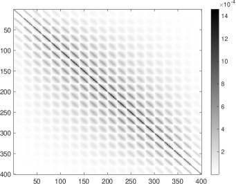
Figure 4.1: Magnitude of the entries of the inverse of $I\otimes A+A\otimes I$ with $A=(n+1)^{2}\operatorname{\operatorname{tridiag}}(-1,2,-1)$ and $n=20$ resulting from a finite difference discretization of the Poisson problem on the unit square

4.4.1 Sparse approximate inverse techniques

We begin by recalling some of the basic ideas behind sparse approximate inverse techniques, as they were outlined in [43, 50, 51]. Given a sparse matrix $M\in\mathbb{R}^{n\times n}$, the problem consists in finding a sparse approximate inverse of $M$ with a prescribed sparsity pattern. Let $S\subseteq\{(i,j)\colon 1\leq i,j\leq n\}$ be a set of pairs of indices defining a sparsity pattern and $\mathcal{S}=\{P\in\mathbb{R}^{n\times n}\colon p_{ij}=0\ (i,j)\notin S\}$ be the associated set of sparse matrices. We then consider the constrained minimization problem

$$\min_{P\in\mathcal{S}}\|I-MP\|_{F}^{2}$$

where the approximate inverse now satisfies a prescribed sparsity. Noticing that $\|I-MP\|_{F}^{2}=\sum_{j=1}^{n}\|e_{j}-Mp_{j}\|_{2}^{2}$, each column of $P$ can be computed separately by solving a sequence of independent least squares problems. Since all columns are treated similarly, we restrict the discussion to a single one, denoted $p_{j}$. Let $\mathcal{J}$ be the set of indices of nonzero entries in $p_{j}$. Since the multiplication $Mp_{j}$ only involves the columns of $M$ associated to indices in $\mathcal{J}$, only the submatrix $M(:,\mathcal{J})$ must be retained, thereby drastically reducing the size of the least squares problem. The problem can be further reduced by eliminating the rows of the submatrix $M(:,\mathcal{J})$ that are identically zero (as they will not affect the least squares solution). Denoting $\mathcal{I}$ the set of indices of nonzero rows, the constrained minimization problem turns into a (much smaller) unconstrained problem

$$\min_{\hat{p}_{j}}\|\hat{e}_{j}-\hat{M}\hat{p}_{j}\|_{2}^{2}$$

where $\hat{M}=M(\mathcal{I},\mathcal{J})$, $\hat{p}_{j}=p_{j}(\mathcal{J})$ and $\hat{e}_{j}=e_{j}(\mathcal{I})$. The greater the sparsity of the matrices, the smaller the size of the least squares problem, which is usually solved exactly using a QR factorization. The procedure is then repeated for each column of $P$. Instead of prescribing the sparsity pattern, several authors have proposed adaptive strategies to iteratively augment it until a prescribed tolerance is reached. For simplicity, we will not consider such techniques here and instead refer to the original articles [43, 50, 51] for further details. It goes without saying that sparse approximate inverse techniques can only be successful if the inverse can be well approximated by a sparse matrix. Although it might seem as a rather restrictive condition, it is frequently met in applications. In the next section, we will combine low Kronecker rank approximations with sparse approximate inverse techniques. In effect, it will allow us to compute low Kronecker rank approximations of the inverse with sparse factor matrices.

4.4.2 Low Kronecker rank sparse approximate inverse

We first consider again the Kronecker rank 1 approximation. We seek factor matrices $C\in\mathcal{S}_{C}$ and $D\in\mathcal{S}_{D}$ where $\mathcal{S}_{C}$ and $\mathcal{S}_{D}$ are sets of sparse matrices with prescribed sparsity defined analogously as in Section 4.4.1. Recalling Equation (4.3) from Section 4.1, we have

$$\|I-\sum_{k=1}^{r}A_{k}C\otimes B_{k}D\|_{F}^{2}=\|\tilde{I}-\mathcal{B}D\|_{F}^{2}=\sum_{j=1}^{m}\|\tilde{e}_{j}-\mathcal{B}d_{j}\|_{2}^{2}.$$

We now proceed analogously to Section 4.4.1 and solve a sequence of independent least squares problems for each column of $D$. Let $\mathcal{J}$ be the set of indices corresponding to nonzero entries of $d_{j}$ and $\mathcal{I}$ be the set of indices for nonzero rows in $\mathcal{B}(:,\mathcal{J})$. We then solve the unconstrained problem

$$\min_{\hat{d}_{j}}\|\hat{e}_{j}-\hat{\mathcal{B}}\hat{d}_{j}\|_{2}^{2}$$ (4.10)

where $\hat{\mathcal{B}}=\mathcal{B}(\mathcal{I},\mathcal{J})$, $\hat{d}_{j}=d_{j}(\mathcal{J})$ and $\hat{e}_{j}=\tilde{e}_{j}(\mathcal{I})$. Contrary to standard sparse approximate inverse techniques, we will not rely on a QR factorization of $\hat{\mathcal{B}}$ but on the normal equations. The solution of the least squares problem in (4.10) is the solution of the linear system $\hat{\mathcal{B}}^{T}\hat{\mathcal{B}}\hat{d}_{j}=\hat{\mathcal{B}}^{T}\hat{e}_{j}$. Furthermore, we notice that

$$\hat{\mathcal{B}}^{T}\hat{\mathcal{B}}=\mathcal{B}(\mathcal{I},\mathcal{J})^{T}\mathcal{B}(\mathcal{I},\mathcal{J})=(\mathcal{B}^{T}\mathcal{B})(\mathcal{J},\mathcal{J}),$$

$$\hat{\mathcal{B}}^{T}\hat{e}_{j}=\mathcal{B}(\mathcal{I},\mathcal{J})^{T}\tilde{e}_{j}(\mathcal{I})=(\mathcal{B}^{T}\tilde{e}_{j})(\mathcal{J}).$$

Therefore, the required system matrix and right-hand side vector are simply submatrices of $\mathcal{B}^{T}\mathcal{B}$ and $\mathcal{B}^{T}\tilde{I}$, respectively. These quantities are formed only once at each iteration and appropriate submatrices are extracted for computing each column of $D$. This strategy is very advantageous given that forming $\mathcal{B}^{T}\mathcal{B}$ is rather expensive. The strategy for computing $C$ is again analogous. Overall, computing sparse factors only requires minor adjustments to Algorithm 1. The case of a Kronecker rank $q$ sparse approximate inverse is not much more difficult. As we have seen in Section 4.2,

$$\|I-\sum_{s=1}^{q}\sum_{k=1}^{r}A_{k}C_{s}\otimes B_{k}D_{s}\|_{F}^{2}=\|\tilde{I}-\mathcal{B}D\|_{F}^{2}$$

where $D=[D_{1};\dots;D_{q}]$ and $\mathcal{B}$ is defined in (4.7). We then apply exactly the same strategy as for the Kronecker rank 1 approximation. The only minor difficulty lies in defining suitable sparsity patterns $\mathcal{S}_{C}$ and $\mathcal{S}_{D}$ that accounts for the sparsity patterns of the individual factor matrices $C_{s}$ and $D_{s}$ stacked in the matrices $C$ and $D$, respectively.

It must be emphasized that sparse approximate inverse techniques are applied to the factor matrices themselves. This strategy is much more efficient than blindly applying the same techniques on the (potentially huge) matrix $M=\sum_{k=1}^{r}A_{k}\otimes B_{k}$. Apart from obvious storage savings, sparse approximate inverses further speed up the application of the preconditioning operator $\mathcal{P}$.

5 Numerical experiments

We now test our preconditioning strategies on a few benchmark problems. All algorithms are implemented in MATLAB R2022b and run on MacOS with an M1 chip and 32 GB of RAM. As a first experiment, we consider the Lyapunov equation

$$AX+XA=C$$ (5.1)

where $A=(n+1)^{2}\operatorname{\operatorname{tridiag}}(-1,2,-1)$ is a symmetric tridiagonal matrix and $C$ is a matrix of all ones. This equation is the prototypical example of a centered finite difference discretization of the Poisson problem on the unit square with homogeneous Dirichlet boundary conditions and $n+2$ discretization points along each direction. Although it is actually a standard Sylvester equation, it serves merely as a validation check. More complicated problems will follow.

We compare the nearest Kronecker product (NKP) preconditioners with (sparse) Kronecker product approximations of the inverse (KINV), as described in Sections 4.1 and 4.2, respectively. We must emphasize that the NKP preconditioners are only defined for Kronecker ranks $q\leq 2$ while the KINV preconditioners may have larger Kronecker ranks. The former are computed using the SVD approach (Algorithm 1) while the latter are obtained after $10$ iterations of alternating least squares (Algorithm 2), which was generally more than enough given the fast convergence of the algorithm. As initial guess, we chose $C_{1}=\operatorname{\operatorname{diag}}(1,1,\dots,1)$ and then defined $C_{s}$ for $s\geq 2$ from $C_{s-1}$ by adding a sub-diagonal and super-diagonal of ones.

Figure 5.1 shows the convergence history of the Gl-GMRES method when solving (5.1) for $n=200$ using the NKP and KINV preconditioners for $q=1$ and $q=1,2,3$, respectively. Since the system matrix in this specific example has Kronecker rank $2$, we have only tested the NKP preconditioner for $q=1$. Moreover, although the operators in this section are symmetric positive definite (i.e. $\mathcal{M}=\mathcal{M}^{T}$ and $\langle\mathcal{M}(X),X\rangle_{F}>0$ for $X\neq 0$), not all preconditioning operators are and therefore oblige us to use non-symmetric solvers such as the right preconditioned Gl-GMRES method described in Section 2. In order to ease comparison, we have used the same method for all experiments with a default tolerance of $10^{-8}$ on the absolute residual and a zero initial matrix. According to Figure 5.1, Kronecker rank $1$ preconditioners marginally improve the convergence but not enough to meet the tolerance after $100$ iterations, our cap in this experiment. However, slightly increasing the Kronecker rank of the KINV preconditioners yields drastic improvements.

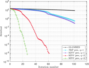
Figure 5.1: Convergence history for solving (5.1) with $n=200$ using the right-preconditioned Gl-GMRES method with NKP and KINV preconditioners

Although increasing the Kronecker rank of the KINV preconditioners reduces the iteration count, the magnitude of the entries of the factor matrices also tends to increase. Figure 5.2 shows the magnitude of the entries of $\sum_{s=1}^{q}|C_{s}|$, i.e. the absolute sum of entries of the factor matrices $C_{s}$. This quantity accounts for all factor matrices and avoids being misled by individual ones (whose numbering is completely arbitrary).

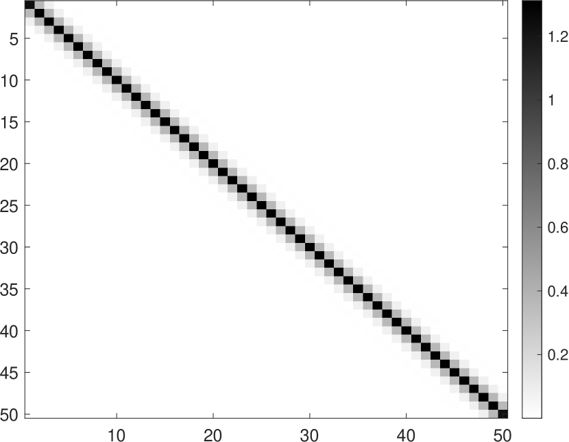
(a) $q=1$

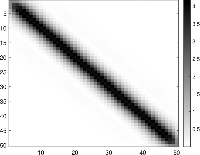
(b) $q=2$

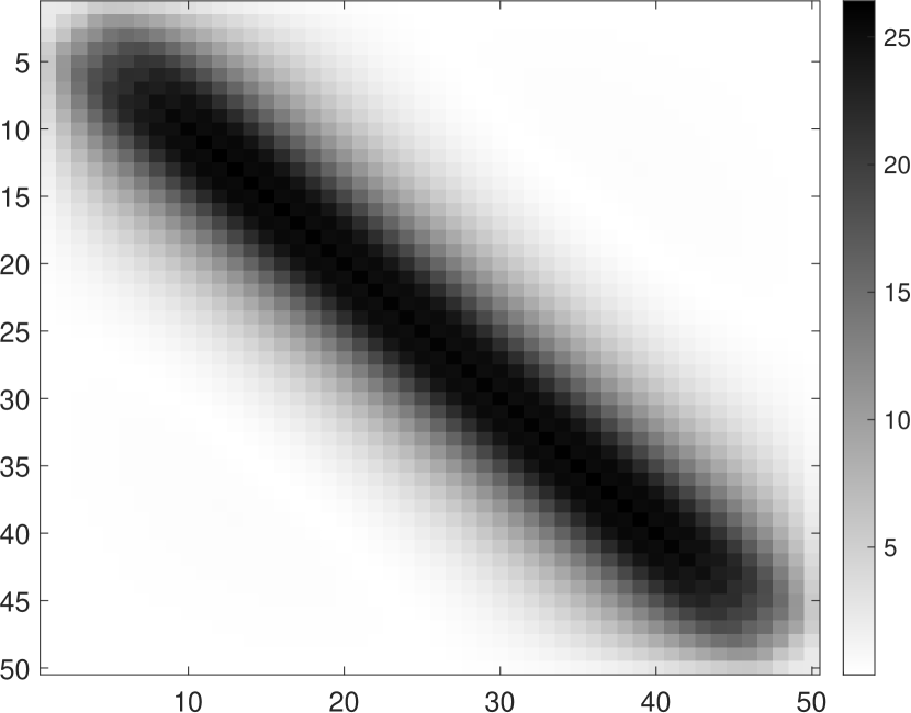
(c) $q=3$

Figure 5.2: Magnitude of the entries of $\sum_{s=1}^{q}|C_{s}|$ for $n=50$

The pattern depicted in Figure 5.2 is not surprising given that the approximate inverse should converge to the actual inverse as the Kronecker rank increases. Unfortunately, it also suggests increasing the bandwidth of sparse approximate inverses as the Kronecker rank increases. We have repeated the experiment in Figure 5.1 for increasing values of $n$ (finer discretizations) and compared a fully dense implementation to a sparse one. Our sparse implementation is combined with sparse approximate inverse techniques described in Section 4.4, where the sparsity pattern is prescribed following the results in Figure 5.2. Iteration counts and computing times for the dense and sparse case are summarized in Tables 1(a) and 1(b), respectively. For the preconditioned methods, the computing time includes the setup time for the preconditioner. Evidently, exploiting sparsity is beneficial for reducing computing times and memory load but the benefits only become visible for sufficiently large problems. The experiment also reveals that the fully dense factor matrices of the approximate inverse are exceedingly well approximated by sparse matrices and lead to nearly the same iteration counts. However, they tend to increase with the size of the problem. For fine grids, the NKP preconditioner actually increases the computing time. Indeed, as already inferred from Figure 5.1, it barely reduces the iteration count while introducing an overhead for solving matrix equations with the preconditioning operator. On the contrary, KINV preconditioners with increased Kronecker ranks can provide effective preconditioning solutions.

$n$	Gl-GMRES	NKP	KINV
50	102 / 0.09	46 / 0.07	10 / 0.06
100	200∗ / 0.55	91 / 0.22	14 / 0.10
200	200∗ / 2.46	183 / 3.26	26 / 0.53
400	200∗ / 10.6	200∗ / 15.2	52 / 3.30
800	200∗ / 60.4	200∗ / 110.2	103 / 24.8

(a) Dense implementation

$n$	Gl-GMRES	NKP	KINV
50	102 / 0.07	46 / 0.04	9 / 0.13
100	200∗ / 0.51	91 / 0.19	14 / 0.28
200	200∗ / 1.47	183 / 1.92	27 / 0.64
400	200∗ / 7.13	200∗ / 14.0	53 / 2.79
800	200∗ / 54.7	200∗ / 102.2	106 / 18.2

(b) Sparse implementation

Table 5.1: Iteration count / computing time (sec) for preconditioned Gl-GMRES with NKP ($q=1$) and KINV ($q=3$). For ^∗ the method did not converge within $200$ iterations

Our next set of experiments arises from applications in isogeometric analysis. Isogeometric analysis is a spline based discretization technique for solving PDEs [23, 52]. Conceived as an extension of the classical finite element method, it relies on spline functions such as B-splines both for parametrizing the geometry and representing the unknown solution. The underlying tensor product structure of the basis functions in dimension $d\geq 2$ naturally leads to Kronecker products on the algebraic level. Given the scope of this work, we will restrict our discussion to dimension $d=2$. In some idealized settings (e.g. rectangular domains and separable coefficient functions), tensorized finite element discretizations of the Poisson model problem lead to solving Sylvester equations

$$B_{1}XA_{1}^{T}+B_{2}XA_{2}^{T}=C$$

where the factor matrices $A_{1},A_{2}$ and $B_{1},B_{2}$ are stiffness or mass matrices of univariate problems [5]. This connection is an immediate consequence of the Kronecker product structure of the stiffness matrix

$$K=A_{1}\otimes B_{1}+A_{2}\otimes B_{2}.$$

Unfortunately, this pleasant structure only holds for idealized problems. For non-trivial single patch geometries, systems matrices (e.g. stiffness and mass matrices) are nevertheless very well approximated by sums of Kronecker products; a property at the heart of several fast assembly algorithms in isogeometric analysis [53, 54, 55]. Recall from Section 3 that the singular value decay of $\mathcal{R}(M)$ indicates how well $M$ can be approximated by a sum of Kronecker products. This decay is shown in Figure 3(b) for the geometry depicted in Figure 3(a) and does not depend on the discretization parameters. Generally speaking, the stiffness matrix has a larger Kronecker rank than the mass matrix, suggesting that NKP preconditioners might work much better for the latter. For this specific example, the mass matrix has Kronecker rank $10$ while the stiffness matrix has Kronecker rank $35$. Fast assembly algorithms such as those described in [53, 54, 55] may compute the factor matrices without ever explicitly assembling the system matrix. We exploit this feature by solving the associated generalized Sylvester equations using again the right preconditioned Gl-GMRES method with the NKP and KINV preconditioners. The latter are computed using only $5$ iterations of alternating least squares.

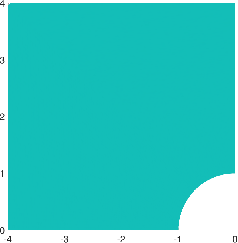
(a) Geometry

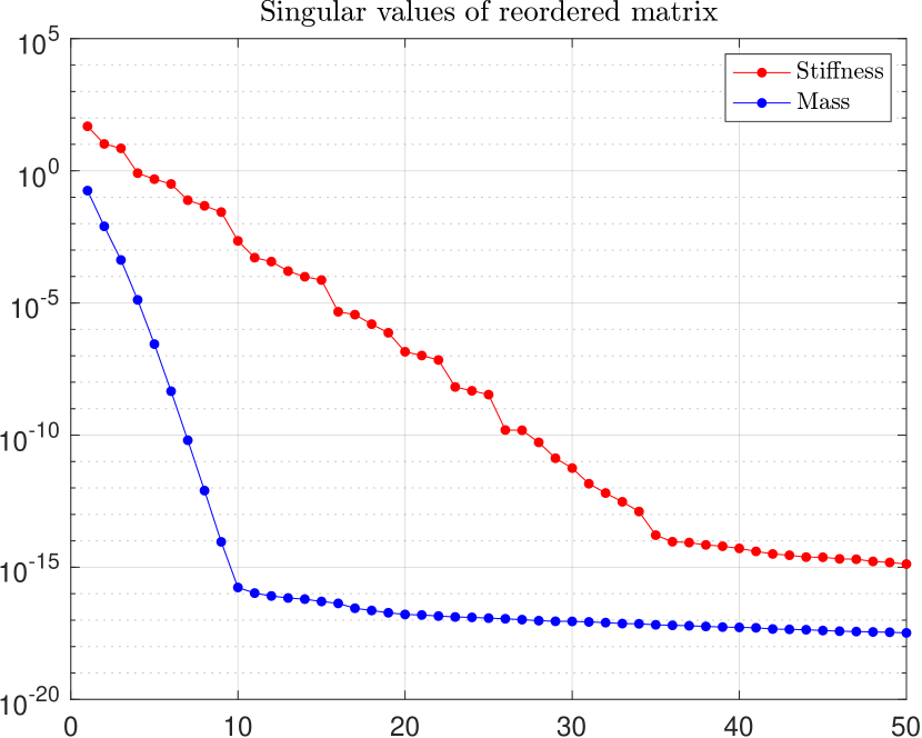
(b) Singular values

Figure 5.3: Plate with a hole

For applications involving PDEs, it is important to design preconditioners that are robust with respect to the discretization parameters (e.g. mesh size and polynomial degree) and physical parameters (e.g. coefficient values). Therefore, we conduct an $hp$-refinement test by decreasing the mesh size $h$ and increasing the spline degree $p$. The iteration counts and computing times are reported in Tables 5.2 and 5.3 for the stiffness and mass operators, respectively, and a right-hand side matrix of all ones. The tolerance was set at $10^{-8}$ and the number of iterations was capped at $500$. Clearly, according to Table 5.2, none of our preconditioning strategies are robust with respect to the mesh size but are nearly robust with respect to the spline degree. Although the iteration counts might be smaller for the NKP preconditioner than for KINV, they are not quite as stable for fine meshes (Table 5.2). Moreover, while the setup cost for the NKP preconditioner is smaller than for KINV, its application cost is larger. Indeed, applying the NKP preconditioning operator requires solving generalized Sylvester equations for $r=2$. In our experiments, we have first transformed them to standard form (which is generally possible) before calling MATLAB’s built-in solver for Sylvester equations. MATLAB’s solver relies on Schur decompositions and is well suited for small to moderate size matrices. Experiments on finer meshes would evidently require different strategies but they fall outside the scope of this paper. Our numerical experiments indicate that the smaller application cost of the KINV preconditioner generally outpaces its larger setup cost. Nevertheless, these conclusions also depend on the origin of the matrix equation and the properties of the underlying system matrix. Indeed, both preconditioning strategies perform remarkably well for the mass operator (Table 5.3).

$h^{-1}$	$p=1$	$p=2$	$p=3$	$p=4$	$p=5$	$p=6$
16	83 / 0.05	65 / 0.02	76 / 0.03	132 / 0.08	240 / 0.37	445 / 1.73
32	189 / 0.24	137 / 0.15	125 / 0.12	171 / 0.22	312 / 0.87	500∗ / 3.32
64	500∗ / 5.5	500∗ / 6.04	300 / 2.23	500∗ / 4.29	500∗ / 4.31	500∗ / 4.26
128	500∗ / 17.1	500∗ / 19.1	500∗ / 20.8	500∗ / 25.6	500∗ / 20.7	500∗ / 21.0

(a) Gl-GMRES

$h^{-1}$	$p=1$	$p=2$	$p=3$	$p=4$	$p=5$	$p=6$
16	19 / 0.11	21 / 0.03	22 / 0.03	22 / 0.04	22 / 0.04	22 / 0.03
32	28 / 0.08	28 / 0.08	29 / 0.08	28 / 0.09	28 / 0.09	28 / 0.09
64	54 / 0.41	47 / 0.39	50 / 0.45	52 / 0.47	50 / 0.46	49 / 0.45
128	500∗ / 40.4	108 / 5.93	219 / 14.0	184 / 13.3	151 / 11.1	394 / 33.5

(b) Gl-GMRES + NKP ($q=2$)

$h^{-1}$	$p=1$	$p=2$	$p=3$	$p=4$	$p=5$	$p=6$
16	24 / 0.09	26 / 0.04	27 / 0.03	29 / 0.04	32 / 0.04	34 / 0.05
32	39 / 0.08	38 / 0.08	40 / 0.09	42 / 0.09	45 / 0.10	49 / 0.10
64	76 / 0.32	71 / 0.36	72 / 0.34	74 / 0.37	76 / 0.37	79 / 0.39
128	154 / 3.45	141 / 3.12	140 / 3.15	141 / 2.59	143 / 2.48	146 / 3.47

(c) Gl-GMRES + KINV ($q=2$)

Table 5.2: Plate with a hole: Iteration count / computing time (sec) for preconditioned Gl-GMRES applied to the stiffness operator. For ^∗ the method did not converge within $500$ iterations

$h^{-1}$	$p=1$	$p=2$	$p=3$	$p=4$	$p=5$	$p=6$
16	38 / 0.02	93 / 0.05	189 / 0.2	332 / 0.77	473 / 2.09	500∗ / 2.28
32	47 / 0.02	119 / 0.12	273 / 0.72	500∗ / 3.05	500∗ / 3.04	500∗ / 3.14
64	52 / 0.08	137 / 0.43	329 / 2.44	500∗ / 6.34	500∗ / 8.31	500∗ / 8.44
128	57 / 0.45	149 / 1.65	363 / 8.17	500∗ / 15.7	500∗ / 15.9	500∗ / 15.77

(a) Gl-GMRES

$h^{-1}$	$p=1$	$p=2$	$p=3$	$p=4$	$p=5$	$p=6$
16	5 / 0.03	5 / 0.01	5 / 0.01	6 / 0.03	6 / 0.01	6 / 0.01
32	6 / 0.02	6 / 0.02	6 / 0.02	6 / 0.02	6 / 0.02	6 / 0.02
64	6 / 0.05	6 / 0.06	6 / 0.06	6 / 0.07	6 / 0.07	6 / 0.07
128	6 / 0.32	6 / 0.36	6 / 0.30	6 / 0.35	6 / 0.33	6 / 0.35

(b) Gl-GMRES + NKP ($q=2$)

$h^{-1}$	$p=1$	$p=2$	$p=3$	$p=4$	$p=5$	$p=6$
16	3 / 0.03	4 / 0.02	4 / 0.02	4 / 0.02	4 / 0.02	4 / 0.02
32	4 / 0.03	4 / 0.03	4 / 0.02	4 / 0.02	4 / 0.03	4 / 0.03
64	4 / 0.06	4 / 0.06	4 / 0.07	4 / 0.07	4 / 0.07	4 / 0.08
128	4 / 0.31	4 / 0.28	4 / 0.28	4 / 0.27	4 / 0.33	4 / 0.33

(c) Gl-GMRES + KINV ($q=2$)

Table 5.3: Plate with a hole: Iteration count / computing time (sec) for preconditioned Gl-GMRES applied to the mass operator. For ^∗ the method did not converge within $500$ iterations

6 Conclusion

In this paper, we have proposed general and algebraic preconditioning techniques for the iterative solution of generalized Sylvester matrix equations. Our strategies rely on low Kronecker rank approximations of either the operator or its inverse. In both cases, the approximations are computed without explicitly forming the associated system matrix and are therefore well suited for large scale applications. Moreover, we have shown how sparse approximate inverse techniques could be combined with low Kronecker rank approximations, thereby speeding up the application of the preconditioning operator. Numerical experiments have shown the effectiveness of our strategies in preconditioning generalized Sylvester equations arising from discretizations of PDEs, including non-trivial problems in isogeometric analysis. Although in this context preconditioning techniques are usually tailored to specific matrices (e.g. the mass or stiffness matrix) our approach is very general and applicable to both, including linear combinations. For this reason, it might also be promising for preconditioning the stages of implicit time integration schemes.

A natural extension of our work would entail solving generalized Sylvester tensor equations [56], as they arise for discretizations of PDEs in three-dimensional space. Extending our methods to this case is a research direction worthwhile exploring.

References

- [1] L. Gao, Kronecker products on preconditioning, Ph.D. thesis, King Abdullah University of Science and Technology (2013).
- [2] L. Gao, V. M. Calo, Fast isogeometric solvers for explicit dynamics, Computer Methods in Applied Mechanics and Engineering 274 (2014) 19–41.
- [3] G. Loli, G. Sangalli, M. Tani, Easy and efficient preconditioning of the isogeometric mass matrix, Computers & Mathematics with Applications (2021).
- [4] L. Gao, V. M. Calo, Preconditioners based on the Alternating-Direction-Implicit algorithm for the 2D steady-state diffusion equation with orthotropic heterogeneous coefficients, Journal of Computational and Applied Mathematics 273 (2015) 274–295.
- [5] G. Sangalli, M. Tani, Isogeometric preconditioners based on fast solvers for the Sylvester equation, SIAM Journal on Scientific Computing 38 (6) (2016) A3644–A3671.
- [6] K.-W. E. Chu, Exclusion theorems and the perturbation analysis of the generalized eigenvalue problem, SIAM journal on numerical analysis 24 (5) (1987) 1114–1125.
- [7] N. J. Higham, Accuracy and stability of numerical algorithms, SIAM, 2002.
- [8] G. W. Stewart, Error and perturbation bounds for subspaces associated with certain eigenvalue problems, SIAM review 15 (4) (1973) 727–764.
- [9] L. Grasedyck, Existence and computation of low Kronecker-rank approximations for large linear systems of tensor product structure, Computing 72 (3) (2004) 247–265.
- [10] D. Kressner, C. Tobler, Krylov subspace methods for linear systems with tensor product structure, SIAM journal on matrix analysis and applications 31 (4) (2010) 1688–1714.
- [11] G. Stewart, J. Sun, Matrix Perturbation Theory, Computer Science and Scientific Computing, ACADEMIC Press, INC, 1990.
- [12] S. Barnett, C. Storey, Some applications of the Lyapunov matrix equation, IMA Journal of Applied Mathematics 4 (1) (1968) 33–42.
- [13] Z. Gajic, M. T. J. Qureshi, Lyapunov matrix equation in system stability and control, Courier Corporation, 2008.
- [14] A. C. Antoulas, Approximation of large-scale dynamical systems, SIAM, 2005.
- [15] M. J. Gander, M. Outrata, Spectral analysis of implicit 2 stage block Runge-Kutta preconditioners, HAL open science (2023).
- [16] V. Simoncini, Computational methods for linear matrix equations, SIAM Review 58 (3) (2016) 377–441.
- [17] R. H. Bartels, G. W. Stewart, Solution of the matrix equation AX+ XB= C [F4], Communications of the ACM 15 (9) (1972) 820–826.
- [18] N. S. Ellner, E. L. Wachspress, New ADI model problem applications, in: Proceedings of 1986 ACM Fall joint computer conference, 1986, pp. 528–534.
- [19] I. Jonsson, B. Kågström, Recursive blocked algorithms for solving triangular systems—Part I: One-sided and coupled Sylvester-type matrix equations, ACM Transactions on Mathematical Software (TOMS) 28 (4) (2002) 392–415.
- [20] U. Baur, Low rank solution of data-sparse Sylvester equations, Numerical Linear Algebra with Applications 15 (9) (2008) 837–851.
- [21] O. G. Ernst, C. E. Powell, D. J. Silvester, E. Ullmann, Efficient solvers for a linear stochastic Galerkin mixed formulation of diffusion problems with random data, SIAM Journal on Scientific Computing 31 (2) (2009) 1424–1447.
- [22] E. Ullmann, A Kronecker product preconditioner for stochastic Galerkin finite element discretizations, SIAM Journal on Scientific Computing 32 (2) (2010) 923–946.
- [23] T. J. Hughes, J. A. Cottrell, Y. Bazilevs, Isogeometric analysis: CAD, finite elements, NURBS, exact geometry and mesh refinement, Computer methods in applied mechanics and engineering 194 (39-41) (2005) 4135–4195.
- [24] K.-w. E. Chu, The solution of the matrix equations AXB- CXD= E AND (YA- DZ, YC- BZ)=(E, F), Linear Algebra and its Applications 93 (1987) 93–105.
- [25] P. Lancaster, Explicit solutions of linear matrix equations, SIAM review 12 (4) (1970) 544–566.
- [26] R. A. Horn, C. R. Johnson, Topics in Matrix Analysis, Cambridge University Press, 1991.
- [27] K. Jbilou, A. Messaoudi, H. Sadok, Global FOM and GMRES algorithms for matrix equations, Applied Numerical Mathematics 31 (1) (1999) 49–63.
- [28] M. Hochbruck, G. Starke, Preconditioned Krylov subspace methods for Lyapunov matrix equations, SIAM Journal on Matrix Analysis and Applications 16 (1) (1995) 156–171.
- [29] Y. Saad, M. H. Schultz, GMRES: A generalized minimal residual algorithm for solving nonsymmetric linear systems, SIAM Journal on scientific and statistical computing 7 (3) (1986) 856–869.
- [30] A. Bouhamidi, K. Jbilou, A note on the numerical approximate solutions for generalized Sylvester matrix equations with applications, Applied Mathematics and Computation 206 (2) (2008) 687–694.
- [31] M. R. Hestenes, E. Stiefel, et al., Methods of conjugate gradients for solving linear systems, Journal of research of the National Bureau of Standards 49 (6) (1952) 409–436.
- [32] Y. Saad, Iterative methods for sparse linear systems, SIAM, 2003.
- [33] H. A. Van der Vorst, Bi-CGSTAB: A fast and smoothly converging variant of Bi-CG for the solution of nonsymmetric linear systems, SIAM Journal on scientific and Statistical Computing 13 (2) (1992) 631–644.
- [34] J. G. Nagy, M. E. Kilmer, Kronecker product approximation for preconditioning in three-dimensional imaging applications, IEEE Transactions on Image Processing 15 (3) (2006) 604–613.
- [35] A. N. Langville, W. J. Stewart, A Kronecker product approximate preconditioner for SANs, Numerical Linear Algebra with Applications 11 (8-9) (2004) 723–752.
- [36] A. N. Langville, W. J. Stewart, The Kronecker product and stochastic automata networks, Journal of computational and applied mathematics 167 (2) (2004) 429–447.
- [37] A. N. Langville, W. J. Stewart, Testing the nearest Kronecker product preconditioner on Markov chains and stochastic automata networks, INFORMS Journal on Computing 16 (3) (2004) 300–315.
- [38] Y. Voet, E. Sande, A. Buffa, A mathematical theory for mass lumping and its generalization with applications to isogeometric analysis, Computer Methods in Applied Mechanics and Engineering 410 (2023) 116033.
- [39] C. F. Van Loan, N. Pitsianis, Approximation with Kronecker products, in: Linear algebra for large scale and real-time applications, Springer, 1993, pp. 293–314.
- [40] G. H. Golub, C. F. Van Loan, Matrix computations, JHU press, 2013.
- [41] J. W. Demmel, Applied numerical linear algebra, SIAM, 1997.
- [42] A. Greenbaum, Iterative methods for solving linear systems, SIAM, 1997.
- [43] M. J. Grote, T. Huckle, Parallel preconditioning with sparse approximate inverses, SIAM Journal on Scientific Computing 18 (3) (1997) 838–853.
- [44] R. A. Horn, C. R. Johnson, Matrix analysis, Cambridge university press, 2012.
- [45] M. Dressler, A. Uschmajew, V. Chandrasekaran, Kronecker product approximation of operators in spectral norm via alternating SDP, arXiv preprint arXiv:2207.03186 (2022).
- [46] S. Demko, W. F. Moss, P. W. Smith, Decay rates for inverses of band matrices, Mathematics of computation 43 (168) (1984) 491–499.
- [47] M. Benzi, G. H. Golub, Bounds for the entries of matrix functions with applications to preconditioning, BIT Numerical Mathematics 39 (3) (1999) 417–438.
- [48] C. Canuto, V. Simoncini, M. Verani, On the decay of the inverse of matrices that are sum of Kronecker products, Linear Algebra and its Applications 452 (2014) 21–39.
- [49] M. Benzi, V. Simoncini, Decay bounds for functions of Hermitian matrices with banded or Kronecker structure, SIAM Journal on Matrix Analysis and Applications 36 (3) (2015) 1263–1282.
- [50] E. Chow, Y. Saad, Approximate inverse preconditioners via sparse-sparse iterations, SIAM Journal on Scientific Computing 19 (3) (1998) 995–1023.
- [51] M. Benzi, M. Tuma, A comparative study of sparse approximate inverse preconditioners, Applied Numerical Mathematics 30 (2-3) (1999) 305–340.
- [52] J. A. Cottrell, T. J. Hughes, Y. Bazilevs, Isogeometric analysis: toward integration of CAD and FEA, John Wiley & Sons, 2009.
- [53] A. Mantzaflaris, B. Jüttler, B. N. Khoromskij, U. Langer, Low rank tensor methods in Galerkin-based isogeometric analysis, Computer Methods in Applied Mechanics and Engineering 316 (2017) 1062–1085.
- [54] F. Scholz, A. Mantzaflaris, B. Jüttler, Partial tensor decomposition for decoupling isogeometric Galerkin discretizations, Computer Methods in Applied Mechanics and Engineering 336 (2018) 485–506.
- [55] C. Hofreither, A black-box low-rank approximation algorithm for fast matrix assembly in isogeometric analysis, Computer Methods in Applied Mechanics and Engineering 333 (2018) 311–330.
- [56] Z. Chen, L. Lu, A projection method and Kronecker product preconditioner for solving Sylvester tensor equations, Science China Mathematics 55 (6) (2012) 1281–1292.