Graph Embedded Intuitionistic Fuzzy RVFL for Class Imbalance Learning

Abstract

The domain of machine learning is confronted with a crucial research area known as class imbalance learning, which presents considerable hurdles in the precise classification of minority classes. This issue can result in biased models where the majority class takes precedence in the training process, leading to the underrepresentation of the minority class. The random vector functional link (RVFL) network is a widely-used and effective learning model for classification due to its speed and efficiency. However, it suffers from low accuracy when dealing with imbalanced datasets. To overcome this limitation, we propose a novel graph embedded intuitionistic fuzzy RVFL for class imbalance learning (GE-IFRVFL-CIL) model incorporating a weighting mechanism to handle imbalanced datasets. The proposed GE-IFRVFL-CIL model has a plethora of benefits, such as $(i)$ it leverages graph embedding to extract semantically rich information from the dataset, $(ii)$ it uses intuitionistic fuzzy sets to handle uncertainty and imprecision in the data, $(iii)$ and the most important, it tackles class imbalance learning. The amalgamation of a weighting scheme, graph embedding, and intuitionistic fuzzy sets leads to the superior performance of the proposed model on various benchmark imbalanced datasets, including UCI and KEEL. Furthermore, we implement the proposed GE-IFRVFL-CIL on the ADNI dataset and achieved promising results, demonstrating the model’s effectiveness in real-world applications. The proposed method provides a promising solution for handling class imbalance in machine learning and has the potential to be applied to other classification problems.

I Introduction

The ability of artificial neural networks (ANNs) to approximate nonlinear mappings is the primary reason for their huge success in many disciplines among numerous machine learning approaches [1]. ANNs have demonstrated success in various fields such as rainfall forecasting [2], clinical medicine [3], stock market predictions [4], solving ordinary and partial differential equations [5, 6, 7], engineering domains [8, 9] and so on. Feedforward neural network (FN) is one of the most popular ANNs. The universal approximation capabilities of standard single layer FN (SLFN) and multilayer FN (MLFN) were discussed rigorously by many researchers [10, 11, 12].

The gradient descent (GD) method, an iterative process, is one of the most often used techniques for optimizing the cost function to train ANNs. In the GD-based technique, the difference between the real output and the anticipated output of the model backpropagates in an effort to optimize the weights and biases of the model. This iterative strategy has a number of underlying issues, such as being time-consuming, slow convergence, having a tendency to converge to local rather than global optima [13], being extremely sensitive to the choice of the learning rate, and the point of initialization to start the iteration.

In the early 1990s, randomized neural networks (RNNs) [14, 15] were proposed to avoid the pitfalls of GD-based neural networks. In RNN, some network parameters are fixed during the training period, and parameters of output layers are calculated via the closed-form solution [16, 17, 18]. Randomized SLFN [14], RVFL network [15], and extreme learning machine (ELM) [19, 20] are among the prominent RNNs. RVFL is distinguished from other RNNs by the direct linkages between the input and output layers. The weights and biases within the hidden layer of the RVFL are randomly generated and kept fixed throughout the training phase. The output parameters, namely direct link weights and the weights connecting the hidden layer to the output layer, are analytically calculated using the Pseudo-inverse or the least-square method. The incorporation of direct links in the RVFL has been observed to significantly improve the learning performance by functioning as a regularization for the randomization [21, 22]. The role of direct links, bias in the output layer, and the domain of random weights and biases are evaluated comprehensively in [21, 23]. Furthermore, the thinner topology of the RVFL, compared to the ELM, aids in reducing its complexity and making it more attractive according to Occam’s principle and probably approximately correct (PAC) learning theory [24, 25]. The RVFL offers fast training speed as well as universal approximation ability [12, 26].

The RVFL delivers encouraging outcomes for a variety of applications, including Alzheimer’s disease diagnosis [27], electricity load demand forecasting [28], visual tracking [29], data streams [30] and so on. Numerous variants of the original RVFL model have been developed to improve its generalization performance. The RVFL model converts the original features to a randomized features, which makes RVFL unstable. A sparse autoencoder with $l1$-norm regularization was employed in RVFL (SP-RVFL) by Zhang et al. [31]. The SP-RVFL deals with the issue of instability caused by randomization and learns the network parameters more appropriately than the traditional RVFL. In [32], the authors presented two models, namely RVFL+ (incorporating RVFL with learning using privileged information (LUPI)) and KRVFL+ (Kernel-based RVFL+). During the training phase, RVFL+ benefits from privileged data in addition to the training data. KRVFL+ manages nonlinear interactions between higher dimensional input and output vectors along with the privileged information. RVFL+ still has the same challenge as RVFL networks: it is challenging to construct the ideal number of hidden nodes. The number of hidden nodes has a major impact on the efficacy of the network’s learning process [33]. Dai et al. [34] developed an algorithm called Incremental RVFL+ (IRVFL+) that is constructive in nature. The IRVFL+ network continually enlarges the hidden nodes of the network to resemble the output. In [35], kernel-based exponentially expanded RVFL (KERVFL) was put forth to avoid the search for an optimal number of hidden nodes by adding the kernel function to the RVFL model. Cao et al. [36] statistically provide a probabilistic interpretation of the robust model under various assumptions regarding distributions of model parameters and outliers. Nevertheless, this method is restricted to estimating a robust loss function using a maximum a posteriori (MAP) pointwise estimate. Scardapane et al. [37] offer two distinct methods for applying full Bayesian inference to the RVFL network.

Certain data points in a dataset that possess qualities and attributes typically associated with one class or category but instead fall into a distinct class or category are known as outliers. The prediction accuracy of machine learning models is severely impacted by noisy data, the presence of outliers, and imbalanced datasets. The class imbalance problem refers to a scenario when there is a substantial disparity in the number of samples pertaining to a particular class in a given dataset compared to the remaining classes. Since the standard RVFL assigns a uniform weighting scheme to each sample while generating the optimal classifier, it is vulnerable to noise, outliers, and imbalanced issues despite its excellent computational efficiency and strong generalization capacity in balanced datasets. The fuzzy theory has been effectively used to mitigate the detrimental effects of noise or outliers on machine learning models’ performance [38, 39]. The fuzzy approach defines a degree membership function by assisting the notion of the distance of data samples to their associated class center. In [40], intuitionistic fuzzy (IF) membership, an extended version of fuzzy membership, was proposed. The IF membership function assigns an IF score to each sample with the help of membership and nonmembership functions. Malik et al. [27] proposed intuitionistic fuzzy RVFL (IFRVFL). For datasets with noise and outliers, IFRVFL outperformed standard RVFL in terms of generalization performance; however, IF theory has not yet addressed the issue of imbalanced datasets.

The original RVFL disregards the geometrical relationship of the data while computing the final output parameters and the randomization process dismantles the topological properties of the dataset [22]. Many improved versions of the RVFL have been proposed as remedies for the aforementioned problem. Li et al. [41] proposed a manifold learning-based variant of RVFL, namely discriminative manifold RVFL (DMRVFL). In order to effectively utilize the intraclass discriminative information and concurrently increase the distances between interclass samples, DMRVFL replaced the inflexible one-hot label matrix with a more flexible soft label matrix. On the one hand, DMRVFL enlarges the distance of the interclass samples. On the other hand, make the intraclass samples more compact. Ganaie et al. [42] presented two multiclass classifiers, namely Class-Var-RVFL and Total-Var-RVFL, which utilize both the original and the projected randomized space’s dispersion of training data to optimize output layer weights. The optimization process involves minimizing both the distribution of training data and the weight norm of output units. The former relies on intraclass variance minimization, while the latter employs total variance minimization. Recently, graph embedded intuitionistic fuzzy weighted RVFL (GE-IFWRVFL) [43] was proposed by incorporating notions of IF and graph embedding (GE) simultaneously with RVFL. Under the context of GE, a suitable regularisation term is applied to the RVFL optimization problem. The suggested regularisation term developed inside the GE framework to facilitate the generation of a compact solution that can be utilized in the calculation of the output weights of a network under various subspace learning (SL) criteria. Although GE-IFRVFL brings forth many benefits, such as it preserves the geometrical property of the dataset and IF assists the model in handling outliers and noisy data samples; however, GE-IFRVFL fails to deal with the imbalanced datasets.

It is possible in reality for patterns of minority class to be more significant than patterns from other classes. For instance, in the case of heart illness, people with symptoms of the condition (minority class) should be regarded as more vital than those whose readings are normal (majority class). Conventional RVFL treats each sample uniformly irrespective of its belongingness to minority or majority classes, and as a result, RVFL is biased in favor of the majority class samples. The penalty of inaccuracies for different classes is frequently unfair and unknown in most imbalanced situations. Thus, class imbalance issues plague RVFL badly and hinder the performance of the model. The improved fuzziness-based RVFL (IF-RVFL) [44] demonstrated the performance of their model in real-life liver disease imbalanced datasets. Class-specific weighted RVFL (CSWRVFL) [45] handles the dilemma of imbalanced datasets and carried out tests to identify the power quality disturbance. Although RVFL has made significant progress in dealing with noise, outliers, and retaining the topological relationship of the data [45, 46], there has been relatively little improvement in dealing with imbalance datasets. To bridge this gap, it becomes necessary to develop a novel variant of RVFL that can effectively handle imbalanced datasets. Therefore, we propose a novel graph embedded intuitionistic fuzzy random vector functional link network for class imbalance learning (GE-IFRVFL-CIL). The GE framework, IF membership functions, and weighting scheme approaches are employed in the proposed GE-IFRVFL-CIL model to address the imbalance issue along with noise, outliers, and geometrical structure preservation of the dataset. This paper’s primary highlights are summarized as follows:

1. The proposed GE-IFRVFL-CIL model incorporates a weighting scheme for class imbalance learning. The weighting scheme takes care of the minority class by assigning unit weightage to its samples, and the weights of the majority class are lowered by the ratio of the number of positive class samples to the number of negative class samples.

2. The proposed GE-IFRVFL-CIL model employs two types of GE frameworks, namely linear discriminant analysis (LDA) [47] and local Fisher discriminant analysis (LFDA) [48], yielding two alternative combinations of models. These GE frameworks, along with the utilization of a regularization term, seek to maintain graph structural information in the projected space, including node similarity, connection, and community structure.

3. IF membership technique is employed in the proposed GE-IFRVFL-CIL model to deal with noisy and outlier samples in the datasets. The degree of membership and non-membership is assigned to each sample in the IF concept to determine if it is a pure sample, noise, or outlier, and data samples are weighted accordingly.

4. We demonstrate the efficiency of the proposed model in the UCI and KEEL imbalanced datasets from various domains. Experiments confirmed that the proposed GE-IFRVFL-CIL-1 and GE-IFRVFL-CIL-2 models are competitive and, in the context of class-imbalanced learning, outperform numerous state-of-the-art models.

5. As an application, the proposed GE-IFRVFL-CIL models are used to detect Alzheimer’s disease. The experimental findings show that the proposed models outperform the baseline models in terms of efficiency and generalization.

The subsequent sections of this paper are arranged as follows. Section II presents a concise introduction to RVFL, IFRVFL, ELM networks, and the GE frameworks. Section III provides the mathematical formulation of the proposed models, followed by a weighting mechanism for class imbalanced learning and two distinct graph weighting techniques, LDA and LFDA, under the GE framework. Experimental results are demonstrated in Section IV on UCI and KEEL datasets and compare them to existing cutting-edge models. We also employ the proposed models to detect Alzheimer’s disease. Section V includes a conclusion to the article and some recommendations for future work.

II Related Works

This section provides a brief overview of the RVFL structure, IFRVFL, ELM networks, and the GE frameworks. Let $\bigl{\{}(x_{k},y_{k})|\,x_{k}\in\mathbb{R}^{p},\,y_{k}\in\mathbb{R}^{q};k=1,\ldots,N\bigl{\}}$ be the training set, where $p$ denotes the number of features in each input sample, and $q$ denotes the number of classes with $N$ training data samples.

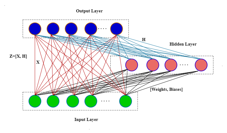
Figure 1: The pictorial representation of the RVFL model.

II-A Random Vector Functional Link (RVFL) Network [15]

The RVFL is a randomized version of the SLFN. The architecture of the RVFL is shown in Fig. 1. The RVFL network comprises three layers: input, hidden, and output layers. All three layers are made up of neurons that are linked together by weights. Biases at the hidden layer and weights from the input layer to the hidden layer are generated at random (that are kept fixed during the training process) from their respective domains $[0,r]$ and $[-r,r]$ respectively, where $r$ is a positive real number. The original features of input samples are also linked with output layers via direct links, and no bias is used in the output layer. Generally, the output weights are calculated analytically via the Moore-Penrose inverse or the least square method. Mathematically, the RVFL model is a function $\varphi:\mathbb{R}^{p}\rightarrow\mathbb{R}^{q}$, and is defined as:

$$\varphi\left(x_{i}\right)=\sum_{k=1}^{p}\beta_{k}x_{ik}+\sum_{k=p+1}^{{p+h_{l}}}\beta_{k}\Phi\left(\left\langle\omega_{k},x_{i}\right\rangle+\xi_{k}\right),\leavevmode\nobreak\ i=1,\ldots,N,$$ (1)

where $x_{i}=\left[x_{i1},x_{i2},\cdots,x_{ip}\right]$ is the $i^{th}$ sample, ${h_{l}}$ is the number of hidden nodes, $\left\langle\omega_{k},x_{i}\right\rangle=$ $\omega_{k}\cdot x_{i}$ is the standard inner product defined on Euclidean space $\mathbb{R}^{p}$, $\beta_{k}=$ $\left[\beta_{k1},\beta_{k2},\cdots,\beta_{kq}\right]$ is the output weight vector which connects all output nodes to the $k^{\text{th }}$ (input) hidden nodes, $1\leq k\leq$ $p+{h_{l}}$, $w_{j}=\left[w_{j1},w_{j2},\cdots,w_{jp}\right]$ is the weight vector connecting all the input nodes to the $j^{\text{th }}$ hidden node, $1\leq j\leq$ $h_{l}$, $\Phi$ is the activation function at the hidden layer and $\xi_{k}$ is the bias term at the $k^{\text{th }}$ hidden node.

Equivalently, we can write the formulation of the RVFL in terms of a matrix equation. For this, let $X\in\mathbb{R}^{N\times p}$ be the input matrix and $Y\in\mathbb{R}^{N\times q}$ be the target matrix. $H_{N\times{h_{l}}}$ is the hidden layer matrix obtained by transforming the input matrix with the help of randomly initialized weights and biases followed by the non-linear activation function $\Phi$, which can be described as:

$$H=\Phi(XW+\xi),$$ (2)

where $W_{p\times{h_{l}}}$ is the randomly initialized weights matrix and $\xi$ is the bias matrix. Therefore, $H$ is written as

$${H}=\left[\begin{array}[]{ccc}\Phi\left(w_{1}\cdot x_{1}+\xi_{1}\right)&\ldots&\Phi\left(w_{h_{l}}\cdot x_{1}+\xi_{h_{l}}\right)\\ \vdots&\ddots&\vdots\\ \Phi\left(w_{1}\cdot x_{N}+\xi_{1}\right)&\ldots&\Phi\left(w_{h_{l}}\cdot x_{N}+\xi_{h_{l}}\right)\end{array}\right]_{N\times{h_{l}}}.$$

The hidden features and input features are concatenated as

$$Z=\left[\begin{array}[]{ll}X&H\end{array}\right]_{N\times(p+h_{l})}.$$ (3)

The output layer’s weights are calculated using the matrix equation

$$Z\beta=Y,$$ (4)

where $\beta_{(p+h_{l})\times q}$ is the weight matrix connecting the input layer and hidden layer to the output layer. Solution of (4) is given as

$$\beta=Z^{\dagger}Y,$$ (5)

where $Z^{\dagger}$ is the Moore-Penrose inverse. The solution (5) of RVFL leads to overfitting [21]. Generally, this issue is resolved by adding the regularization term to the optimization problem. The optimization problem of the regularized RVFL is given by

$$\beta_{\min}=\underset{{\beta}}{\text{argmin}}\,\frac{C}{2}\|Z\beta-Y\|_{2}^{2}+\frac{1}{2}\|\beta\|_{2}^{2},$$ (6)

where $C$ is a regularization parameter.

$$\beta_{\min}=\left\{\begin{array}[]{ll}\left({Z}^{T}{Z}+\frac{1}{C}I\right)^{-1}{Z}^{T}{Y},&(p+h_{l})\leq N,\vspace{3mm}\\ {Z}^{T}\left({Z}{Z}^{T}+\frac{1}{C}I\right)^{-1}{Y},&N<(p+h_{l}),\end{array}\right.$$ (7)

where $I$ is an identity matrix of conformal dimension.

II-B Intuitionistic Fuzzy Random Vector Functional Link (IFRVFL) Network [27]

The conventional RVFL model is susceptible to outliers and noise. The intuitionistic fuzzy membership (IFM) [40] technique used by the IFRVFL architecture efficiently tackles the noise and outliers present in the dataset. Let $\bigl{\{}(x_{k},y_{k},\alpha_{k},{\alpha_{k}}^{*})|\,x_{k}\in\mathbb{R}^{p},\,y_{k}\in\mathbb{R}^{q},\,\alpha_{k}\in\mathbb{R},\,{\alpha_{k}}^{*}\in\mathbb{R};k\in\{1,\ldots,N\}\bigl{\}}$ be the fuzzy training set along with the corresponding degree of membership $\alpha_{k}$ and degree of nonmembership ${\alpha_{k}}^{*}$ of each training sample $x_{k}$. The score function based on IFN is defined as

$$\rho_{k}=\left\{\begin{array}[]{lll}{\alpha_{k}},&{\alpha_{k}}^{*}=0,\vspace{3mm}\\ 0,&\alpha_{k}\leq{\alpha_{k}}^{*},\vspace{3mm}\\ \frac{1-{\alpha_{k}}^{*}}{2-{\alpha_{k}}-{\alpha_{k}}^{*}},&\text{otherwise}.\end{array}\right.$$ (8)

The optimization problem of the IFRVFL is given by

$$\beta_{\min}=\underset{{\beta}}{\text{argmin}}\,\frac{1}{2}C\|S(Z\beta-Y)\|_{2}^{2}+\frac{1}{2}\|\beta\|_{2}^{2},$$ (9)

where $S=diag(\rho_{1},\rho_{2},\ldots,\rho_{N})$. The optimization problem (9) is a quadratic and a convex programming problem. As a result, this problem has a unique global optimum solution. The solution of (9) is given by

$$\beta_{\min}=\left\{\begin{array}[]{l}\left({(SZ)}^{T}{(SZ)}+\frac{1}{C}I\right)^{-1}{(SZ)}^{T}{SY},\leavevmode\nobreak\ (p+h_{l})\leq N,\vspace{3mm}\\ {Z}^{T}\left({Z}{Z}^{T}+\frac{1}{C}S^{-1}S^{-1}\right)^{-1}{Y},\leavevmode\nobreak\ N<(p+h_{l}).\end{array}\right.$$ (10)

II-C Extreme Learning Machine [20]

ELM is one of the most popular RNNs. The distinguishing factor between the topology of ELM and RVFL is the presence of direct connections from the input to the output layer in RVFL, whereas such connections are absent in ELM. The optimization problem of the regularized ELM is given by

$$\beta_{\min}=\underset{{\beta}}{\text{argmin}}\,\frac{C}{2}\|H\beta-Y\|_{2}^{2}+\frac{1}{2}\|\beta\|_{2}^{2}.$$ (11)

The solution of (11) is given by

$$\beta_{\min}=\left\{\begin{array}[]{ll}\left({H}^{T}{H}+\frac{1}{C}I\right)^{-1}{H}^{T}{Y},&h_{l}\leq N,\vspace{3mm}\\ {H}^{T}\left({H}{H}^{T}+\frac{1}{C}I\right)^{-1}{Y},&N<h_{l}.\end{array}\right.$$ (12)

II-D Graph Embedding

Although the driving forces behind dimensional reduction algorithms differ, they all have the same goals: to provide a reduced dimensional representation and make the classification work easier. Yan et al. [49] proposed a GE algorithm that reformulates several dimensionality reduction methods within a unified framework and also aids in the design of new algorithms. The embedding process aims to preserve important structural information of the graph, such as node similarity, connectivity, and community structure, in the resulting vector space. In GE, for input dataset $X=\bigl{\{}x_{k}\leavevmode\nobreak\ |\ x_{k}\in\mathbb{R}^{p},\;k=1,\ldots,N\bigl{\}}$, the intrinsic graph, $\mathcal{G}^{int}=\{X,\Delta^{int}\}$, and the penalty graph $\mathcal{G}^{pen}=\{X,\Delta^{pen}\}$ are defined. The weights relating to the unique association between two vertices in $X$ are included in the similarity weight matrix $\Delta^{int}\in\mathbb{R}^{N\times N}$. Each component of the penalty weight matrix, $\Delta^{pen}\in\mathbb{R}^{N\times N}$ is the penalty matrix of $X$ that takes into account a particular relationship between the vertices of the graph. The graph embedding optimization problem is defined as follows:

$$\hat{v}= \underset{Tr({v_{0}^{T}X^{T}\mathcal{U}X{v_{0}})}=c}{\rm argmin}\sum_{k\neq l}\left\|{{v_{0}}^{T}{x}_{k}-{v_{0}}^{T}{x}_{l}}\right\|_{2}^{2}\Delta_{kl}^{int}$$

$$= \underset{Tr({{v_{0}}^{T}{X}^{T}\mathcal{U}{X}{v_{0}})}=c}{\rm argmin}{Tr({v_{0}}^{T}{X}^{T}{\mathcal{L}}{X}{v_{0}})}.$$ (13)

Here, the operator $Tr()$ denotes the trace of a matrix, $v_{0}$ is the projection matrix, $\mathcal{L}=\mathcal{D}-\Delta^{int}\in\mathbb{R}^{N\times N}$ is the graph Laplacian matrix of the intrinsic graph $\mathcal{G}^{int}$ and the elements of the diagonal matrix $\mathcal{D}$ is defined as $\mathcal{D}_{kk}=\sum_{l}\Delta_{kl}^{int}$. $\mathcal{U}=\mathcal{L}^{p}=\mathcal{D}^{p}-\Delta^{pen}$ is the Laplacian matrix of penalty graph $\mathcal{G}^{pen}$ or a diagonal matrix for normalizing scale, and $c$ is a constant value. The optimization problem (II-D) boils down to a generalized eigenvalue problem [50],

$${G}_{i}{s}=\lambda{G}_{p}{s},$$ (14)

here, $G_{i}=X^{T}\mathcal{L}X$ and ${G}_{p}=X^{T}\mathcal{U}X$. It implies that the transformation matrix will be formed by the eigenvectors of matrix $G={G}_{p}^{-1}{G}_{i}$. The matrix $G$ takes into account data samples’ intrinsic and penalty graph connections simultaneously.

III Proposed Graph Embedded Intuitionistic Fuzzy RVFL for Class Imbalance Learning (GE-IFRVFL-CIL)

This section gives a detailed description of the proposed model GE-IFRVFL-CIL. We first define the formulation of the proposed model. In the proposed work, a weighting algorithm is employed for class imbalance learning, as well as two types of GE frameworks, namely LDA [47] and LFDA [48]. A regularization term is also used under the GE framework that manages the topological properties of the data. We combine the weighting strategy with both GE frameworks and present two models to cope with imbalanced datasets as a consequence. The optimization problem of the proposed GE-IFRVFL-CIL model is defined as follows:

$$\underset{\beta}{min}\leavevmode\nobreak\ \leavevmode\nobreak\ \frac{1}{2}\norm{\beta}_{2}^{2}+\frac{\theta}{2}\norm{G^{\frac{1}{2}}\beta}_{2}^{2}+\frac{C}{2}(d_{+})\norm{S_{+}^{\frac{1}{2}}\xi_{+}}_{2}^{2}+$$

$$\frac{C}{2}(d_{-})\norm{S_{-}^{\frac{1}{2}}\xi_{-}}_{2}^{2},$$

$$s.t.\leavevmode\nobreak\ \leavevmode\nobreak\ Z_{pos}\beta=Y_{+}-\xi_{+},$$

$$Z_{neg}\beta=Y_{-}-\xi_{-}.$$ (15)

Here, $\beta$ is the weight matrix connecting the hidden layer and the input layer to the output layer, $\theta$ is a graph regularization parameter, $G$ is the graph embedding matrix defined in Subsection II-D, $S_{-}$ ($S_{+}$) is the diagonal matrices with IF scores along its diagonal for the negative (positive) class samples. $\xi_{-}$ ($\xi_{+}$) is the error vector of the negative (positive) class samples. Here, $d_{-}$ ($d_{+}$) is the weighting scheme of the negative (positive) class defined in Subsection III-A. $C\in\mathbb{R^{+}}$ is the regularization parameter to penalize the error variables. $Z_{neg}$ ($Z_{pos}$) denotes the non-linear as well as linear projection of the negative (positive) class samples. which is defined as

$$Z_{neg}=\left[\begin{array}[]{ll}X_{-}&H_{neg}\end{array}\right],$$ (16)

$$Z_{pos}=\left[\begin{array}[]{ll}X_{+}&H_{pos}\end{array}\right],$$ (17)

where $X_{-}\leavevmode\nobreak\ (X_{+})$ is the negative (positive) class’ input matrix and $H_{neg}\leavevmode\nobreak\ (H_{pos})$ is the negative (positive) class’ hidden layer matrix obtained by transforming $X_{-}\leavevmode\nobreak\ (X_{+})$ with the help of randomly initialized weights and biases followed by the non-linear activation function $\Phi$. $Y_{-}$ ($Y_{+}$) is the target matrix for the negative (positive) class samples. The Lagrangian of (III) is given as follows:

$$L= \frac{1}{2}\norm{\beta}_{2}^{2}+\frac{\theta}{2}\norm{G^{\frac{1}{2}}\beta}_{2}^{2}+\frac{C}{2}(d_{+})\norm{S_{+}^{\frac{1}{2}}\xi_{+}}_{2}^{2}+$$

$$\frac{C}{2}(d_{-})\norm{S_{-}^{\frac{1}{2}}\xi_{-}}_{2}^{2}-\alpha_{+}^{T}(Z_{pos}\beta-Y_{+}+\xi_{+})-$$

$$\alpha^{T}_{-}(Z_{neg}\beta-Y_{-}+\xi_{-}),$$ (18)

where $\alpha_{+}$ and $\alpha_{-}$ are the Lagrange multipliers. Let

$$l_{pos}=C\times d_{+}\text{ and }l_{neg}=C\times d_{-}.$$ (19)

Rewriting (III), we have

$$L= \frac{1}{2}\norm{\beta}^{2}_{2}+\frac{\theta}{2}\norm{G^{\frac{1}{2}}\beta}^{2}_{2}+\frac{l_{pos}}{2}\norm{S_{+}^{\frac{1}{2}}\xi_{+}}^{2}_{2}+$$

$$\frac{l_{neg}}{2}\norm{S_{-}^{\frac{1}{2}}\xi_{-}}^{2}_{2}-\begin{bmatrix}\alpha^{T}_{+}&\alpha^{T}_{-}\end{bmatrix}\Bigg{(}\begin{bmatrix}Z_{pos}\\ Z_{neg}\end{bmatrix}\beta-$$

$$\begin{bmatrix}Y_{+}\\ Y_{-}\end{bmatrix}+\begin{bmatrix}\xi_{+}\\ \xi_{-}\end{bmatrix}\Bigg{)}.$$ (20)

By applying K.K.T. conditions to (III), we have

$$\beta+\theta G\beta-(Z^{T}_{pos}\alpha_{+}+Z^{T}_{neg}\alpha_{-})=0,$$ (21)

$$l_{pos}S_{+}\xi_{+}-\alpha_{+}=0,$$ (22)

$$l_{neg}S_{-}\xi_{-}-\alpha_{-}=0,$$ (23)

$$Z_{pos}\beta-Y_{+}+\xi_{+}=0,$$ (24)

$$Z_{neg}\beta-Y_{-}+\xi_{-}=0.$$ (25)

Rewriting the equations (21), (22) and (23), we have

$$(I+\theta G)\beta=(Z^{T}_{pos}\alpha_{+}+Z^{T}_{neg}\alpha_{-}),$$ (26)

$$l_{pos}S_{+}\xi_{+}=\alpha_{+},$$ (27)

$$l_{neg}S_{-}\xi_{-}=\alpha_{-},$$ (28)

where $I$ is an identity matrix of conformal dimensions. Using (27) and (28) in (26), we have

$$(I+\theta G)\beta= l_{pos}Z^{T}_{pos}S_{+}\xi_{+}+l_{neg}Z^{T}_{neg}S_{-}\xi_{-},$$ (29)

$$(I+\theta G)\beta= l_{pos}Z^{T}_{pos}S_{+}(Y_{+}-Z_{pos}\beta)+$$

$$\leavevmode\nobreak\ l_{neg}Z^{T}_{neg}S_{-}(Y_{-}-Z_{neg}\beta),$$ (30)

$$(I+\theta G+l_{pos}Z^{T}_{pos}S_{+}Z_{pos}+l_{neg}Z^{T}_{neg}S_{-}Z_{neg})\beta$$

$$=l_{pos}Z^{T}_{pos}S_{+}Y_{+}+l_{neg}Z^{T}_{neg}S_{-}Y_{-},$$ (31)

Multiply $(\frac{1}{l_{pos}}+\frac{1}{l_{neg}})$ to (III), we have

$$\Bigg{(}\frac{1}{l_{pos}}+\frac{1}{l_{neg}}\Bigg{)}\Bigg{(}I+\theta G+l_{pos}Z^{T}_{pos}S_{+}Z_{pos}+l_{neg}Z^{T}_{neg}S_{-}Z_{neg}\Bigg{)}\beta$$

$$=\Bigg{(}\frac{1}{l_{pos}}+\frac{1}{l_{neg}}\Bigg{)}\Bigg{(}l_{pos}Z^{T}_{pos}S_{+}Y_{+}+l_{neg}Z^{T}_{neg}S_{-}Y_{-}\Bigg{)},$$ (32)

$$\Bigg{(}\Big{(}\frac{1}{l_{pos}}+\frac{1}{l_{neg}}\Big{)}\Big{(}I+\theta G\Big{)}+Z^{T}_{pos}S_{+}Z_{pos}+\frac{l_{neg}}{l_{pos}}Z^{T}_{neg}S_{-}Z_{neg}+$$

$$\frac{l_{pos}}{l_{neg}}Z^{T}_{pos}S_{+}Z_{pos}+Z^{T}_{neg}S_{-}Z_{neg}\Bigg{)}\beta=Z^{T}_{pos}S_{+}Y_{+}+$$

$$\frac{l_{neg}}{l_{pos}}Z^{T}_{neg}S_{-}Y_{-}+\frac{l_{pos}}{l_{neg}}Z^{T}_{pos}S_{+}Y_{+}+Z^{T}_{neg}S_{-}Y_{-},$$ (33)

$$\beta=\Bigg{(}\Big{(}\frac{1}{l_{pos}}+\frac{1}{l_{neg}}\Big{)}\Big{(}I+\theta G\Big{)}+Z^{T}_{pos}S_{+}Z_{pos}+\frac{l_{neg}}{l_{pos}}Z^{T}_{neg}S_{-}Z_{neg}+$$

$$\frac{l_{pos}}{l_{neg}}Z^{T}_{pos}S_{+}Z_{pos}+Z^{T}_{neg}S_{-}Z_{neg}\Bigg{)}^{-1}\Bigg{(}Z^{T}_{pos}S_{+}Y_{+}+\frac{l_{neg}}{l_{pos}}Z^{T}_{neg}S_{-}Y_{-}+$$

$$\frac{l_{pos}}{l_{neg}}Z^{T}_{pos}S_{+}Y_{+}+Z^{T}_{neg}S_{-}Y_{-}\Bigg{)},$$ (34)

$$\beta=\Bigg{(}\Big{(}\frac{1}{l_{pos}}+\frac{1}{l_{neg}}\Big{)}\Big{(}I+\theta G\Big{)}+(1+\frac{l_{pos}}{l_{neg}})Z^{T}_{pos}S_{+}Z_{pos}\leavevmode\nobreak\ +$$

$$(1+\frac{l_{neg}}{l_{pos}})Z^{T}_{neg}S_{-}Z_{neg}\Bigg{)}^{-1}\Bigg{(}(1+\frac{l_{pos}}{l_{neg}})Z^{T}_{pos}S_{+}Y_{+}\leavevmode\nobreak\ +$$

$$(1+\frac{l_{neg}}{l_{pos}})Z^{T}_{neg}S_{-}Y_{-}\Bigg{)},$$ (35)

$$\beta=\Bigg{(}\big{(}\frac{1}{l_{pos}}+\frac{1}{l_{neg}}\big{)}\big{(}I+\theta G\big{)}+[Z_{pos}^{T},\leavevmode\nobreak\ Z_{neg}^{T}]$$

$$\begin{bmatrix}(1+\frac{l_{pos}}{l_{neg}})S_{+}&\bm{0}\\ \bm{0}&(1+\frac{l_{neg}}{l_{pos}})S_{-}\end{bmatrix}\begin{bmatrix}Z_{pos}\\ Z_{neg}\end{bmatrix}\Bigg{)}^{-1}$$

$$\begin{bmatrix}Z_{pos}^{T}&Z_{neg}^{T}\end{bmatrix}\begin{bmatrix}(1+\frac{l_{pos}}{l_{neg}})S_{+}&\bm{0}\\ \bm{0}&(1+\frac{l_{neg}}{l_{pos}})S_{-}\end{bmatrix}\begin{bmatrix}Y_{+}\\ Y_{-}\end{bmatrix}.$$ (36)

As stated, the proposed model uses a weighting scheme for class imbalance learning and two types of GE frameworks. Consequent subsections define the weighting algorithm and GE frameworks.

III-A Class Imbalance Weighting Scheme [51]

Let $l_{n}$ ($l_{p}$) denote the number of samples of the negative (positive) class.

$$d_{+} =1,\leavevmode\nobreak\ \text{if}\leavevmode\nobreak\ x_{i}\leavevmode\nobreak\ \text{is in the positive class,}$$ (37)

$$d_{-} =\frac{l_{p}}{l_{n}},\leavevmode\nobreak\ \text{if}\leavevmode\nobreak\ x_{i}\leavevmode\nobreak\ \text{is in the negative class}.$$ (38)

In this weighting method, the sample of the minority class is given unit weights, and the weight of the majority class is reduced by a factor equal to the proportion of positive class samples to negative class samples.

III-B Graph Embedding Frameworks for the Proposed GE-IFRVFL-CIL Model

Both the intrinsic as well as penalty graphs are based on the concatenated matrix $Z$, i.e., $\mathcal{G}^{int}=\{Z,\Delta^{int}\}$ and $\mathcal{G}^{pen}=\{Z,\Delta^{pen}\}$. Therefore, ${G}_{i}=Z^{T}\mathcal{L}Z$ and ${G}_{p}=Z^{T}\mathcal{U}Z$. Weights for intrinsic and penalty graphs are specified in the literature for the LDA [47] and LFDA [48] as follows:

• Linear discriminant analysis (LDA): The intrinsic and penalty graph weights for the LDA model are as follows:

  $$\Delta^{int}_{ij} =\left\{\begin{array}[]{ll}\frac{1}{l_{c_{i}}},&\text{if}\leavevmode\nobreak\ \leavevmode\nobreak\ c_{i}=c_{j},\vspace{3mm}\\ 0,&\text{otherwise}.\end{array}\right.$$ (41)

  $$\Delta^{pen}_{ij} =\left\{\begin{array}[]{ll}\frac{1}{N}-\frac{1}{l_{c_{i}}},&\text{if}\leavevmode\nobreak\ \leavevmode\nobreak\ c_{i}=c_{j},\vspace{3mm}\\ \frac{1}{N},&\text{otherwise}.\end{array}\right.$$ (44)

  Here, $l_{c_{i}}$ denotes the number of samples in the class $c_{i}$.

• Local Fisher discriminant analysis (LFDA): LFDA model assigns intrinsic and penalty graph weights as follows:

  $$\Delta^{int}_{ij} =\left\{\begin{array}[]{ll}\frac{\eta_{ij}}{l_{c_{i}}},&\text{if}\leavevmode\nobreak\ \leavevmode\nobreak\ c_{i}=c_{j},\vspace{3mm}\\ 0,&\text{otherwise}.\end{array}\right.$$ (47)

  $$\Delta^{pen}_{ij} =\left\{\begin{array}[]{ll}\eta_{ij}\bigg{(}\frac{1}{N}-\frac{1}{l_{c_{i}}}\bigg{)},&\text{if}\leavevmode\nobreak\ \leavevmode\nobreak\ c_{i}=c_{j},\vspace{3mm}\\ \frac{1}{N},&\text{otherwise}.\end{array}\right.$$ (50)

  Here, $\eta_{ij}=exp(-\frac{\norm{z_{j}-z_{i}}^{2}}{\sigma^{2}})$, where $z_{j},\leavevmode\nobreak\ z_{i}\in Z$ and $\sigma$ is the scaling parameter. The similarity between $z_{j}\leavevmode\nobreak\ \text{and}\leavevmode\nobreak\ z_{i}$ in the matrix $Z$ is measured by $\eta_{ij}$.

To effectively contend with the challenge of imbalanced datasets, we used a weighting scheme in conjunction with two distinct graph embedding techniques, namely LDA and LFDA. From now onwards, GE-IFRVFL-CIL with LDA structure is referred to as GE-IFRVFL-CIL-1, and GE-IFRVFL-CIL with LFDA structure is referred to as GE-IFRVFL-CIL-2.

IV Experiments and Results

To test the efficacy of proposed models, i.e., GE-IFRVFL-CIL-1 and GE-IFRVFL-CIL-2, we compare them to baseline models using publicly available UCI [52] and KEEL [53] imbalanced benchmark datasets from diverse domains. Moreover, we implement the proposed models on the Alzheimer’s disease (AD) dataset, available on the Alzheimer’s Disease Neuroimaging Initiative (ADNI) ($adni.loni.usc.edu$).

IV-A Setup for Experiments

The experimental procedures were executed on a computing system possessing MATLAB R2017b software, an Intel(R) Xeon(R) CPU E5-2697 v4 processor operating at 2.30 GHz with 128-GB Random Access Memory (RAM), and a Windows-10 operating platform. To generate IF weights in IFKRR [54], IFRVFL [27], GE-IFWRVFL [43] and IFTWSVM [39] models, the Gaussian kernel function is employed to project the input samples onto a higher-dimensional space. The Gaussian kernel is defined as: $K(x_{1},x_{2})=exp(-\frac{\norm{x_{1}-x_{2}}^{2}}{\mu^{2}})$, where $\mu$ is the kernel parameter. A random partition is applied to the dataset, dividing it into two subsets for the purposes of testing and training. Specifically, the partitioning follows a proportion of $30:70$ between the testing and training subsets, respectively. To optimize hyperparameter settings for different models, a grid search approach is utilized, which uses $5$-fold cross-validation. This entails the random partitioning of the dataset into five distinct, non-overlapping subsets. In each iteration, one subset is set aside for testing while the remaining four are utilized for training. The final accuracy of each model is reported by evaluating its performance under the best hyperparameter settings. Each model’s parameters are selected from the set: $C=\{10^{-5},10^{-4},\cdots,10^{4},10^{5}\}$, while the hidden nodes numbers, $h_{l}$, are chosen from within the range of $3:20:203$.

Table I: The classification AUCs of the proposed GE-IFRVFL-CIL-1 and GE-IFRVFL-CIL-2 models along with the existing models, i.e., IFTWSVM, IFKRR, ELM, RVFL, IFRVFL and GE-IFWRVFL on UCI [52] and KEEL [53] imbalanced benchmark datasets.

Dataset	IFTWSVM [39]	IFKRR [54]	ELM [20]	RVFL [15]	IFRVFL [27]	GE-IFWRVFL [43]	GE-IFRVFL-CIL-1	GE-IFRVFL-CIL-2
abalone9-18	0.7502	0.7022	0.6614	0.7035	0.7683	0.8272	0.8319	0.8272
cleve	0.8216	0.7422	0.8371	0.851	0.7725	0.8189	0.8189	0.7797
crossplane150	1	0.5873	0.9893	0.9643	0.9821	0.9821	0.9821	1
ecoli-0-2-3-4_vs_5	0.9211	0.9825	0.9965	0.8912	0.9211	0.9912	0.9825	0.9649
ecoli-0-2-6-7_vs_3-5	0.6667	0.6288	0.9333	1	0.9924	1	0.9924	0.9773
ecoli-0-3-4-6_vs_5	0.8083	0.825	0.795	0.8333	0.8333	0.825	0.8333	0.825
ecoli-0-6-7_vs_3-5	0.8833	0.9125	0.8983	0.9375	0.9833	0.875	0.9292	0.8125
ecoli-0-6-7_vs_5	0.7336	0.7172	0.8169	0.75	0.7923	0.8087	0.8675	0.8347
ecoli2	0.8571	0.8087	0.6926	0.8072	0.9341	0.9451	0.9271	0.8996
ecoli4	0.8691	0.8897	0.8959	0.8845	0.8948	0.8845	0.8845	0.8845
glass2	0.8065	0.5	0.7121	0.8105	0.8145	0.5565	0.8387	0.7258
glass5	0.4922	0.7031	0.7453	0.7188	0.7188	0.7266	0.7813	0.9766
haber	0.5588	0.5891	0.5822	0.5253	0.6097	0.6138	0.6085	0.5938
led7digit-0-2-4-5-6-7-8-9_vs_1	0.9016	0.5	0.9073	0.9419	0.9258	0.9258	0.9339	0.9258
monk2	0.8706	0.5	0.7993	0.7961	0.5593	0.7918	0.8059	0.7778
new-thyroid1	0.9444	0.9825	0.9947	1	0.9825	1	1	1
pima	0.7582	0.6886	0.73	0.7452	0.7827	0.8048	0.8035	0.787
shuttle-6_vs_2-3	0.75	0.9394	0.9985	1	0.9924	1	1	1
shuttle-c0-vs-c4	1	1	0.9892	0.9865	0.9865	0.9865	0.9865	1
vehicle1	0.7859	0.7366	0.7626	0.7683	0.7954	0.8367	0.8339	0.7997
vehicle2	0.9819	0.9738	0.9889	0.9893	0.9758	0.9893	0.9893	0.9706
votes	0.9558	0.5	0.9665	0.9715	0.943	0.9558	0.9623	0.9558
vowel	0.9482	0.8279	0.7582	0.8704	0.8631	0.8333	0.8889	0.8704
yeast-0-2-5-7-9_vs_3-6-8	0.9345	0.5	0.9036	0.881	0.9188	0.9122	0.9104	0.8912
yeast-0-3-5-9_vs_7-8	0.5574	0.5926	0.6126	0.4926	0.5963	0.5444	0.7	0.5981
yeast-2_vs_4	0.9507	0.5	0.8172	0.7822	0.915	0.8109	0.8581	0.9326
yeast3	0.8175	0.5	0.8124	0.8192	0.9031	0.912	0.9034	0.9298
ecoli-0-1_vs_5	0.8868	0.8259	0.8303	0.8259	0.8333	0.8184	0.8259	0.8259
ecoli-0-1-4-6_vs_5	0.9321	0.9938	0.9963	1	0.9753	1	1	1
ecoli-0-1-4-7_vs_2-3-5-6	0.9174	0.8391	0.83	0.8	0.8446	0.85	0.85	0.8
Average AUC	0.8354	0.7330	0.8418	0.8449	0.8603	0.8609	0.8843	0.8722
Average Rank	4.8667	6.5167	4.8000	4.6667	4.3167	3.8833	2.9000	4.0500

The following statistical measures are used to assess the algorithms:

AUC $$=\frac{1+T_{+}\text{rate}-F_{+}\text{rate}}{2},$$ (51)

Seny.  (Sensitivity) $$=\frac{T_{+}}{T_{+}+F_{-}},$$ (52)

Spey.  (Specificity) $$=\frac{T_{-}}{T_{-}+F_{+}},$$ (53)

Pren.  (Precision) $$=\frac{T_{+}}{T_{+}+F_{+}},$$ (54)

G-mean $$=\sqrt{\text{Pren.}\times\text{Seny.}},$$ (55)

F-measure $$=2\times\frac{\text{Pren.}\times\text{Seny.}}{\text{Pren.}+\text{Seny.}}.$$ (56)

In this context, the terms false positive ($F_{+}$), true positive ($T_{+}$), false negative ($F_{-}$), and true negative ($T_{-}$) are used to represent different outcomes.

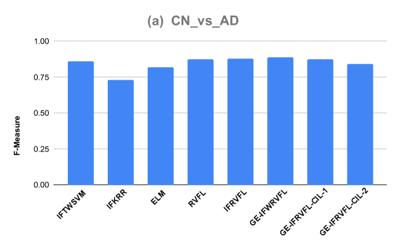
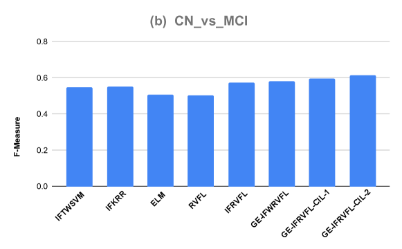
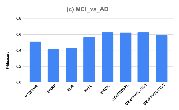
Figure 2: Performance comparison of classification models on ADNI data using F-Measure analysis

IV-B Evaluation on KEEL and UCI benchmark datasets

We use the $30$ standard benchmark datasets from KEEL imbalanced dataset repository [53] and UCI repository [52] of the diverse domains to show the effectiveness of the proposed models for class imbalance learning. We compare the proposed GE-IFRVFL-CIL-1 and GE-IFRVFL-CIL-2 models with various machine learning models, namely intuitionistic fuzzy twin support vector machine (IFTWSVM) [39], RVFL [15], intuitionistic fuzzy kernel ridge regression (IFKRR) [54], ELM [19], IFRVFL [27] and GE-IFWRVFL [43]. Area under the curve (AUC) values from Table I show the performance of the models in classifying data. We follow five metrics namely average AUC, ranking scheme, Friedman test, Nemenyi post hoc test, and win-tie-loss sign test [55] based on analysis and statistical tests for an overall comparison of the models listed in Table I.

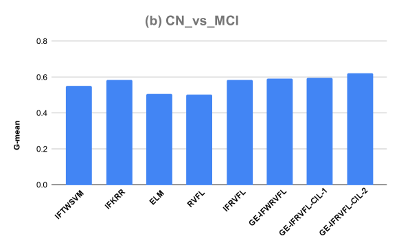
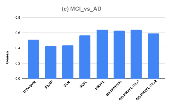
Figure 3: Performance comparison of classification models on ADNI data using G-Mean analysis

Average AUC: Table I shows the classification AUCs of the proposed GE-IFRVFL-CIL-1 and GE-IFRVFL-CIL-2 models along with the existing models IFTWSVM, IFKRR, ELM, RVFL, IFRVFL, and GE-IFWRVFL. Using table I, the average AUC of the existing models, represented as (AUC, model name), are ($83.54\%$, IFTWSVM), ($73.30\%$, IFKRR), ($84.18\%$, ELM), ($84.49\%$, RVFL), ($86.03\%$, IFRVFL) and ($86.09\%$, GE-IFWRVFL). Whereas the AUC values of proposed GE-IFRVFL-CIL-1 and GE-IFRVFL-CIL-2 models are $88.43\%$ and $87.22\%$, better than that of the existing baseline models. The results show that the proposed models, GE-IFRVFL-CIL-1 and GE-IFRVFL-CIL-2, obtained the first and second spots in terms of average AUC and the algorithms of the RVFL family, i.e., GE-IFWRVFL, IFRVFL and RVFL models took the third, fourth and fifth spots, respectively. The number of ELM, IFTWSVM, and IFKRR comes later. Although ELM performs better amongst the non-RVFL models, the proposed GE-IFRVFL-CIL-1 model has $4.25\%$ greater AUC than that of ELM. Thus, the overall results demonstrate the superiority of the proposed algorithms.
Ranking scheme: Although average AUC can be a flawed metric, superior performance in one dataset may compensate for inferior performance in others. To keep this flaw in mind, the models are ranked individually for each dataset to evaluate their respective performances. In this ranking scheme [55], each model is assessed based on its performance on individual datasets: the worst-performing model receives a higher rank, and the best-performing model is ranked lower. Suppose $d$ models are being evaluated using $K$ datasets, and the $l^{th}$ model’s rank on the $k^{th}$ dataset is denoted by $\mathcal{r}^{k}_{l}$. The $l^{th}$ model’s average (overall) rank is determined by the following calculation

$$\mathcal{R}_{l}=\frac{\sum_{k=1}^{K}\mathcal{r}^{k}_{l}}{K}.$$ (57)

The average rank of the models, represented as (average rank, model name), are ($2.9000$, GE-IFRVFL-CIL-1), ($3.8833$, GE-IFWRVFL), ($4.0500$, GE-IFRVFL-CIL-2), ($4.8667$, IFTWSVM), ($6.5167$, IFKRR), ($4.8000$, ELM), ($4.6667$, RVFL) and ($4.3167$, IFRVFL). The proposed GE-IFRVFL-CIL-1 model has a lower average rank (secured first place) than the competing models, and the proposed GE-IFRVFL-CIL-2 secured third place; a lower rank represents better performance of the model.
Friedman test: The Friedman test [56, 57] is used to statistically analyze the models. The models’ average rank is equal under the null hypothesis, assuming they perform equally. The Friedman test follows the chi-squared distribution ($\chi^{2}_{F}$) with $d-1$ degrees of freedom (d.o.f.), where $d$ is the number of models being compared.

$$\chi^{2}_{F} =\frac{12K}{d(d+1)}\left(\sum_{l=1}^{d}\mathcal{R}_{l}^{2}-\frac{d(d+1)^{2}}{4}\right)\leavevmode\nobreak\ \leavevmode\nobreak\ \text{and}$$ (58)

$$F_{F} =\frac{(K-1)\chi_{F}^{2}}{K(d-1)-\chi_{F}^{2}},$$ (59)

where the distribution of $F_{F}$  has $(d-1)$  and $(K-1)(d-1)$  d.o.f.. For $d=8$ and $K=30$, we get $\chi^{2}_{F}=38.03$ and $F_{F}=6.41$. According to the statistical $F-$distribution table, $F_{F}(7,203)=2.05$ at $5\%$ level of significance. As $6.41>2.05$, we reject the null hypothesis. The models differ significantly as a result.
Nemenyi post hoc test: Using the Nemenyi post hoc test [55], we determine whether there is a significant difference between the models. The critical difference $(C.D.)$ is given by

$$C.D.=q_{\alpha}\left(\sqrt{\frac{d(d+1)}{6K}}\right),$$ (60)

where $q_{\alpha}$ is the critical value for the two-tailed Nemenyi test from the distribution table. After calculation, we get $C.D.=1.92.$ The models are deemed to be considerably different if there is a $C.D.$ or greater gap in their average ranks. The average rank differences of proposed GE-IFRVFL-CIL-1 and GE-IFRVFL-CIL-2 from IFKRR are $3.6167,\leavevmode\nobreak\ \text{and}\leavevmode\nobreak\ 2.4667$, respectively. The differences are more than the $C.D.$; therefore, according to Nemenyi post hoc test, the proposed models GE-IFRVFL-CIL-1 and GE-IFRVFL-CIL-2 significantly differ from the IFKRR and therefore, both the proposed models have superior performance than IFKRR. Nevertheless, the GE-IFRVFL-CIL-1 and GE-IFRVFL-CIL-2 model does not significantly vary from other existing models, as determined by the Nemenyi test. However, it is evident that the proposed GE-IFRVFL-CIL-1 outperforms all the existing baseline models and the GE-IFRVFL-CIL-2 model outperforms the existing baseline models (except GE-IFWRVFL), as indicated by their superior average rank.
Win–tie–loss sign test: In research and data analysis, “win-tie-loss” [55] is a popular statistical test to assess whether there is a statistical difference between the outcomes of two or more models. In addition to the above statistical test, we perform win-tie-loss to compare the proposed models with the baseline models. As per the win-tie-loss test, two models are considered to exhibit the same level of performance under the null hypothesis, resulting in both models being successful on $K/2$ out of $K$ datasets. In order for two models to be considered significantly different, each must have at least $K/2+1.96\sqrt{K}/2$ victories. In the event of a tie, the score is evenly split between the models under consideration. For $K=30$, $K/2+1.96\sqrt{K}/2=20.37$. In Table II, the win-tie-loss of models are examined pairwise. In our case, if any of the two models wins on at least $20$ datasets, the two models are statistically different. It has been ascertained that the proposed GE-IFRVFL-CIL-1 has $21$ (w.r.t. IFTWSVM), $23$ (w.r.t. ELM) and $26$ (w.r.t. IFKRR) wins out of $30$ datasets, therefore substantiating its superiority over the existing models. Furthermore, the GE-IFRVFL-CIL-1 model shows considerable differentiation from other models, such as IFTWSVM, IFKRR, and ELM, as affirmed by the outcomes of the win-tie-loss sign test. The proposed GE-IFRVFL-CIL-$2$ model has $22$ (w.r.t. IFKRR) wins out of $30$ datasets, thus establishing its superiority over the baseline models. Although it exhibits a notable level of differentiation from the IFKRR model, it fails to demonstrate a significant distinction from other baseline models. Nonetheless, GE-IFRVFL-CIL-$2$’s winning percentage remains indicative of its efficacy over the baseline models.

The findings exhibit that the utilization of the weighting technique leads to a marked improvement in the generalization performance of GE-IFRVFL-CIL models on imbalanced datasets. Furthermore, the comprehensive analysis affirms that the generalization performance of the proposed GE-IFRVFL-CIL models is significantly enhanced by the integration of GE frameworks, weighting technique, and IF theory when compared to the baseline models.

Table II: Pairwise win-tie-loss of proposed and existing models on UCI [52] and KEEL [53] imbalanced benchmark datasets.

	IFTWSVM [39]	IFKRR [54]	ELM [20]	RVFL [15]	IFRVFL [27]	GE-IFWRVFL [43]	GE-IFRVFL-CIL-1
IFKRR [54]	[10,1,19]
ELM [20]	[15,0,15]	[22,0,8]
RVFL [15]	[15,0,15]	[22,1,7]	[17,0,13]
IFRVFL [27]	[18,1,11]	[26,1,3]	[16,0,14]	[17,3,10]
GE-IFWRVFL [43]	[17,1,12]	[24,1,5]	[16,0,14]	[14,7,9]	[18,3,9]
GE-IFRVFL-CIL-1	[21,0,9]	[26,2,2]	[23,0,7]	[17,8,5]	[19,4,7]	[13,9,8]
GE-IFRVFL-CIL-2	[17,3,10]	[22,3,5]	[19,0,11]	[14,7,9]	[18,1,11]	[10,8,12]	[5,5,20]

Table III: Performance of proposed as well as existing models on ADNI Data.

Subjects	IFTWSVM [39]	IFKRR [54]	ELM [20]	IFRVFL [27]	RVFL [15]	GE-IFWRVFL [43]	GE-IFRVFL-CIL-1	GE-IFRVFL-CIL-2
	(AUC, Seny.)	(AUC, Seny.)	(AUC, Seny.)	(AUC, Seny.)	(AUC, Seny.)	(AUC, Seny.)	(AUC, Seny.)	(AUC, Seny.)
	(Spey., Pren.)	(Spey., Pren.)	(Spey., Pren.)	(Spey., Pren.)	(Spey., Pren.)	(Spey., Pren.)	(Spey., Pren.)	(Spey., Pren.)
CN_vs_AD	$(0.8801,0.9245)$	$(0.7737,0.6981)$	$(0.8444,0.834)$	$(0.898,0.9057)$	$(0.8903,0.8491)$	$(0.9049,0.9057)$	$(0.8912,0.9057)$	$(0.8655,0.8679)$
	$(0.8356,0.8033)$	$(0.8493,0.7708)$	$(0.8548,0.8083)$	$(0.8904,0.8571)$	$(0.9315,0.9)$	$(0.9041,0.8727)$	$(0.8767,0.8421)$	$(0.863,0.8214)$
CN_vs_MCI	$(0.6623,0.5902)$	$(0.6329,0.8361)$	$(0.6318,0.5246)$	$(0.6763,0.6885)$	$(0.6295,0.5246)$	$(0.681,0.7213)$	$(0.6986,0.6393)$	$(0.7122,0.7213)$
	$(0.7344,0.5143)$	$(0.4297,0.4113)$	$(0.7391,0.4894)$	$(0.6641,0.4941)$	$(0.7344,0.4848)$	$(0.6406,0.4889)$	$(0.7578,0.5571)$	$(0.7031,0.5366)$
MCI_vs_AD	$(0.6212,0.4923)$	$(0.5787,0.3538)$	$(0.5858,0.3662)$	$(0.6813,0.8)$	$(0.6621,0.5385)$	$(0.6805,0.7538)$	$(0.6813,0.8)$	$(0.6681,0.6308)$
	$(0.75,0.5333)$	$(0.8036,0.5111)$	$(0.8054,0.5263)$	$(0.5625,0.5149)$	$(0.7857,0.5932)$	$(0.6071,0.5269)$	$(0.5625,0.5149)$	$(0.7054,0.5541)$
Average AUC	$0.7212$	$0.6618$	$0.6873$	$0.7519$	$0.7273$	$\bm{0.7555}$	$\bm{0.757}$	$0.7486$
Here, AUC denotes the area under the curve, Seny. denotes sensitivity, Spey. denotes specificity, Pren. denotes precision.
The boldface in the Average AUC row denotes the performance of the top two models.

IV-C Evaluation on ADNI Dataset

Alzheimer’s disease (AD) is a brain dysfunction illness that gradually impairs people’s memory and cognitive abilities. In order to train the proposed models GE-IFRVFL-CIL-1 and GE-IFRVFL-CIL-2, we use scans from the Alzheimer’s Disease Neuroimaging Initiative (ADNI) dataset, which is accessible at $adni.loni.usc.edu$. The ADNI project was started in 2003 with the intention of examining neuroimaging techniques such as magnetic resonance imaging (MRI), positron emission tomography (PET), and other diagnostic tests of AD at the stage of mild cognitive impairment (MCI). The dataset consists of three cases: control normal (CN) versus moderate cognitive impairment (MCI) (CN_vs_MCI), MCI versus AD (MCI_vs_AD), and CN versus AD (CN_vs_AD).

The AUC values of the proposed GE-IFRVFL-CIL models as well as existing models for AD diagnosis are shown in Table III. We analyze that with an average AUC of $75.70\%$, the proposed GE-IFRVFL-CIL-1 is the best classifier. The AUC of the remaining models, IFTWSVM, IFKRR, ELM, RVFL, IFRVFL GE-IFWRVFL, and GE-IFRVFL-CIL-2, are $72.12\%$, $66.18\%$, $68.73\%$, $72.73\%$, $75.19\%$, $75.55\%$ and $74.86\%$, respectively. In comparison to the AUC of IFKRR, the proposed models (GE-IFRVFL-CIL-1 and GE-IFRVFL-CIL-2) have an average AUC that is around $9.52\%$ and $8.68\%$ higher, respectively. With an AUC of $71.22\%$ in the CN_vs_MCI case, the proposed GE-IFRVFL-CIL-2 came out on top followed by the proposed GE-IFRVFL-CIL-1, which has an AUC of $69.86\%$. With $68.13\%$ AUC value, the proposed GE-IFRVFL-CIL-1 model and the existing IFRVFL model are the most accurate classifiers for the MCI_vs_AD comparison. Therefore, the proposed GE-IFRVFL-CIL-1 model has an overall winning performance, whereas the proposed GE-IFRVFL-CIL-2 wins in the CN_vs_MCI subject and comes under the top four models in terms of overall performance. Of all models, IFKRR has the lowest average AUC, followed by ELM. The top five models (in terms of average AUC) across all the compared models are from the RVFL family, demonstrating the superior generalization capabilities and dominance of the RVFL-based models.

The F-measure analysis is very helpful when evaluating a model’s performance on both positive and negative scenarios and when it needs to avoid favoring one metric over another. It offers a thorough assessment of the accuracy of a binary classification model by concurrently taking precision and recall into account. From Fig. 2 (a) CN_vs_AD, the F-measure analysis shows that the proposed GE-IFRVFL-CIL-1 model has the competitive performance w.r.t. baseline models. From Fig. 2 (b) CN_vs_MCI, the F-measure of the proposed GE-IFRVFL-CIL-2 is the highest, whereas the F-measure of the proposed GE-IFRVFL-CIL-1 is in the second place. From Fig. 2 (c) MCI_vs_AD, the F-measure of the proposed GE-IFRVFL-CIL-1 and IFRVFL model secured the first position. Thus, F-measure analysis also attests to the superiority of the proposed models.

In the context of statistical tests, the geometric mean (G-mean) is less susceptible to extreme values compared to other types of averages, such as the arithmetic mean. Based on Fig. 3 (a) CN_vs_AD, the F-measure analysis indicates that the performance of the proposed GE-IFRVFL-CIL-1 model is almost on par with that of the baseline models, demonstrating its competitive nature. From Fig. 3 (b) CN_vs_MCI, we observe that the G-mean of the proposed GE-IFRVFL-CIL-2 and GE-IFRVFL-CIL-1 models has the highest and second highest value, respectively. The proposed GE-IFRVFL-CIL-1 and IFRVFL models achieved the highest G-mean in the MCI_vs_AD comparison, as shown in Fig. 3 (c). The statistical tests provide further evidence that the proposed models outperformed all other models in the AD diagnosis and achieved the highest rankings in both G-mean and F-measure analyses.

V Conclusion and Future Work

The conundrum of class imbalance poses a formidable challenge for machine learning models, including the conventional RVFL model, thereby impeding their efficacy in accurately classifying minority classes. The traditional RVFL treats every instance in a uniform manner, regardless of its affiliation with either the majority or minority classes, resulting in a biased model that favors the majority class at the expense of the minority class. We proposed novel GE-IFRVFL-CIL-1 and GE-IFRVFL-CIL-2 models to address the predicament of imbalance classification problems. Both the proposed models leverage graph embedding, intuitionistic fuzzy sets, and a weighting mechanism to handle imbalance issues, noisy samples, and outliers in the datasets while simultaneously conserving the inherent geometric structure of the data. The efficacy of the proposed models for class imbalance learning is demonstrated through their application to $30$ standard benchmark datasets sourced from the KEEL imbalanced dataset repository and the UCI repository across a range of diverse domains. By conducting statistical analyses, including the average AUC, ranking scheme, Friedman test, Nemenyi post hoc test, and win-tie-loss sign test, the proposed GE-IFRVFL-CIL-1 and GE-IFRVFL-CIL-2 models have demonstrated superiority over other classifiers. In order to demonstrate the efficacy and generic nature of the proposed GE-IFRVFL-CIL-1 and GE-IFRVFL-CIL-2 models, we applied them to the ADNI dataset for the purpose of diagnosing Alzheimer’s disease. Upon analysis, it is determined that the proposed GE-IFRVFL-CIL-1 model exhibited the highest degree of classification performance as measured by the average AUC metric. As per the findings of the research [58], it was concluded that the MCI versus AD subject represents the most challenging issue to be addressed in the context of diagnosing Alzheimer’s disease. Notwithstanding, the proposed model achieved the foremost position in this scenario, thus exhibiting its superiority over other models. the proposed model GE-IFRVFL-CIL-2 was found to be the most effective in diagnosing CN_vs_MCI subjects, closely followed by the GE-IFRVFL-CIL-1 model. In this paper, our study was focused on shallow RVFL, which has limited potential to capture the intricate relationships among the data. Our forthcoming plan is to expand this research to deep and ensemble variations of RVFL. The present study focuses on binary classification; however, the extension of the proposed model to multi-class classification is an interesting avenue for future research.

References

- Abiodun et al. [2018] O. I. Abiodun, A. Jantan, A. E. Omolara, K. V. Dada, N. A. Mohamed, and H. Arshad, “State-of-the-art in artificial neural network applications: A survey,” Heliyon, vol. 4, no. 11, p. e00938, 2018.
- Luk et al. [2001] K. C. Luk, J. E. Ball, and A. Sharma, “An application of artificial neural networks for rainfall forecasting,” Mathematical and Computer Modelling, vol. 33, no. 6-7, pp. 683–693, 2001.
- Baxt [1995] W. G. Baxt, “Application of artificial neural networks to clinical medicine,” The Lancet, vol. 346, no. 8983, pp. 1135–1138, 1995.
- Dase and Pawar [2010] R. Dase and D. Pawar, “Application of artificial neural network for stock market predictions: A review of literature,” International Journal of Machine Intelligence, vol. 2, no. 2, pp. 14–17, 2010.
- Lagaris et al. [1998] I. E. Lagaris, A. Likas, and D. I. Fotiadis, “Artificial neural networks for solving ordinary and partial differential equations,” IEEE Transactions on Neural Networks, vol. 9, no. 5, pp. 987–1000, 1998.
- Lagaris et al. [2000] I. E. Lagaris, A. C. Likas, and D. G. Papageorgiou, “Neural-network methods for boundary value problems with irregular boundaries,” IEEE Transactions on Neural Networks, vol. 11, no. 5, pp. 1041–1049, 2000.
- Ni and Dong [2022] N. Ni and S. Dong, “Numerical computation of partial differential equations by hidden-layer concatenated extreme learning machine,” arXiv preprint arXiv:2204.11375, 2022.
- Himmelblau [2000] D. M. Himmelblau, “Applications of artificial neural networks in chemical engineering,” Korean Journal of Chemical Engineering, vol. 17, no. 4, pp. 373–392, 2000.
- Flood and Kartam [1994] I. Flood and N. Kartam, “Neural networks in civil engineering. i: Principles and understanding,” Journal of Computing in Civil Engineering, vol. 8, no. 2, pp. 131–148, 1994.
- Hornik et al. [1989] K. Hornik, M. Stinchcombe, and H. White, “Multilayer feedforward networks are universal approximators,” Neural Networks, vol. 2, no. 5, pp. 359–366, 1989.
- Leshno et al. [1993] M. Leshno, V. Y. Lin, A. Pinkus, and S. Schocken, “Multilayer feedforward networks with a nonpolynomial activation function can approximate any function,” Neural Networks, vol. 6, no. 6, pp. 861–867, 1993.
- Igelnik and Pao [1995] B. Igelnik and Y.-H. Pao, “Stochastic choice of basis functions in adaptive function approximation and the functional-link net,” IEEE Transactions on Neural Networks, vol. 6, no. 6, pp. 1320–1329, 1995.
- Gori and Tesi [1992] M. Gori and A. Tesi, “On the problem of local minima in backpropagation,” IEEE Transactions on Pattern Analysis and Machine Intelligence, vol. 14, no. 1, pp. 76–86, 1992.
- Schmidt et al. [1992] W. F. Schmidt, M. A. Kraaijveld, and R. P. Duin, “Feed forward neural networks with random weights,” in International Conference on Pattern Recognition. IEEE Computer Society Press, 1992, pp. 1–1.
- Pao et al. [1994] Y.-H. Pao, G.-H. Park, and D. J. Sobajic, “Learning and generalization characteristics of the random vector functional-link net,” Neurocomputing, vol. 6, no. 2, pp. 163–180, 1994.
- Zhang and Suganthan [2016a] L. Zhang and P. N. Suganthan, “A survey of randomized algorithms for training neural networks,” Information Sciences, vol. 364, pp. 146–155, 2016.
- Cao et al. [2018] W. Cao, X. Wang, Z. Ming, and J. Gao, “A review on neural networks with random weights,” Neurocomputing, vol. 275, pp. 278–287, 2018.
- Suganthan and Katuwal [2021] P. N. Suganthan and R. Katuwal, “On the origins of randomization-based feedforward neural networks,” Applied Soft Computing, vol. 105, p. 107239, 2021.
- Huang et al. [2004] G.-B. Huang, Q.-Y. Zhu, and C.-K. Siew, “Extreme learning machine: a new learning scheme of feedforward neural networks,” in 2004 IEEE International Joint Conference on Neural Networks (IEEE Cat. No.04CH37541), vol. 2, 2004, pp. 985–990 vol.2.
- Huang et al. [2006] ——, “Extreme learning machine: theory and applications,” Neurocomputing, vol. 70, no. 1-3, pp. 489–501, 2006.
- Zhang and Suganthan [2016b] L. Zhang and P. N. Suganthan, “A comprehensive evaluation of random vector functional link networks,” Information Sciences, vol. 367, pp. 1094–1105, 2016.
- Malik et al. [2023] A. K. Malik, R. Gao, M. A. Ganaie, M. Tanveer, and P. N. Suganthan, “Random vector functional link network: recent developments, applications, and future directions,” Applied Soft Computing, Elsevier, 2023.
- Vuković et al. [2018] N. Vuković, M. Petrović, and Z. Miljković, “A comprehensive experimental evaluation of orthogonal polynomial expanded random vector functional link neural networks for regression,” Applied Soft Computing, vol. 70, pp. 1083–1096, 2018.
- Kearns and Vazirani [1994] M. J. Kearns and U. Vazirani, An introduction to computational learning theory. MIT press, 1994.
- Shi et al. [2021] Q. Shi, R. Katuwal, P. N. Suganthan, and M. Tanveer, “Random vector functional link neural network based ensemble deep learning,” Pattern Recognition, vol. 117, p. 107978, 2021.
- Needell et al. [2020] D. Needell, A. A. Nelson, R. Saab, and P. Salanevich, “Random vector functional link networks for function approximation on manifolds,” arXiv preprint arXiv:2007.15776, 2020.
- Malik et al. [2022, DOI: 10.1109/TCSS.2022.3146974] A. K. Malik, M. A. Ganaie, M. Tanveer, P. N. Suganthan, and A. D. N. I. Initiative, “Alzheimer’s disease diagnosis via intuitionistic fuzzy random vector functional link network,” IEEE Transactions on Computational Social Systems, pp. 1–12, 2022, DOI: 10.1109/TCSS.2022.3146974.
- Ren et al. [2016] Y. Ren, P. N. Suganthan, N. Srikanth, and G. Amaratunga, “Random vector functional link network for short-term electricity load demand forecasting,” Information Sciences, vol. 367, pp. 1078–1093, 2016.
- Zhang and Suganthan [2016c] L. Zhang and P. N. Suganthan, “Visual tracking with convolutional random vector functional link network,” IEEE Transactions on Cybernetics, vol. 47, no. 10, pp. 3243–3253, 2016.
- Pratama et al. [2018] M. Pratama, P. P. Angelov, E. Lughofer, and M. J. Er, “Parsimonious random vector functional link network for data streams,” Information Sciences, vol. 430, pp. 519–537, 2018.
- Zhang et al. [2019] Y. Zhang, J. Wu, Z. Cai, B. Du, and S. Y. Philip, “An unsupervised parameter learning model for RVFL neural network,” Neural Networks, vol. 112, pp. 85–97, 2019.
- Zhang and Yang [2020] P.-B. Zhang and Z.-X. Yang, “A new learning paradigm for random vector functional-link network: RVFL+,” Neural Networks, vol. 122, pp. 94–105, 2020.
- Li et al. [2017] J. Li, C. Hua, Y. Yang, and X. Guan, “Bayesian block structure sparse based T-S fuzzy modeling for dynamic prediction of hot metal silicon content in the blast furnace,” IEEE Transactions on Industrial Electronics, vol. 65, no. 6, pp. 4933–4942, 2017.
- Dai et al. [2022] W. Dai, Y. Ao, L. Zhou, P. Zhou, and X. Wang, “Incremental learning paradigm with privileged information for random vector functional-link networks: IRVFL+,” Neural Computing and Applications, vol. 34, no. 9, pp. 6847–6859, 2022.
- Chakravorti and Satyanarayana [2020] T. Chakravorti and P. Satyanarayana, “Non linear system identification using kernel based exponentially extended random vector functional link network,” Applied Soft Computing, vol. 89, p. 106117, 2020.
- Cao et al. [2015] F. Cao, H. Ye, and D. Wang, “A probabilistic learning algorithm for robust modeling using neural networks with random weights,” Information Sciences, vol. 313, pp. 62–78, 2015.
- Scardapane et al. [2017] S. Scardapane, D. Wang, and A. Uncini, “Bayesian random vector functional-link networks for robust data modeling,” IEEE Transactions on Cybernetics, vol. 48, no. 7, pp. 2049–2059, 2017.
- Lin and Wang [2002] C.-F. Lin and S.-D. Wang, “Fuzzy support vector machines,” IEEE Transactions on Neural Networks, vol. 13, no. 2, pp. 464–471, 2002.
- Rezvani et al. [2019] S. Rezvani, X. Wang, and F. Pourpanah, “Intuitionistic fuzzy twin support vector machines,” IEEE Transactions on Fuzzy Systems, vol. 27, no. 11, pp. 2140–2151, 2019.
- Ha et al. [2013] M. Ha, C. Wang, and J. Chen, “The support vector machine based on intuitionistic fuzzy number and kernel function,” Soft Computing, vol. 17, no. 4, pp. 635–641, 2013.
- Li et al. [2021] X. Li, Y. Yang, N. Hu, Z. Cheng, and J. Cheng, “Discriminative manifold random vector functional link neural network for rolling bearing fault diagnosis,” Knowledge-Based Systems, vol. 211, p. 106507, 2021.
- Ganaie et al. [2020] M. A. Ganaie, M. Tanveer, and P. N. Suganthan, “Minimum variance embedded random vector functional link network,” in Neural Information Processing: 27th International Conference, ICONIP 2020, Bangkok, Thailand, November 18–22, 2020, Proceedings, Part V 27. Springer, 2020, pp. 412–419.
- Malik et al. [2022] A. K. Malik, M. A. Ganaie, and M. Tanveer, “Graph embedded intuitionistic fuzzy weighted random vector functional link network,” in 2022 IEEE Symposium Series on Computational Intelligence (SSCI). IEEE, 2022, pp. 293–299.
- Cao et al. [2020] W. Cao, P. Yang, Z. Ming, S. Cai, and J. Zhang, “An improved fuzziness based random vector functional link network for liver disease detection,” in 2020 IEEE 6th Intl Conference on Big Data Security on Cloud (BigDataSecurity), IEEE Intl Conference on High Performance and Smart Computing, (HPSC) and IEEE Intl Conference on Intelligent Data and Security (IDS), 2020, pp. 42–48.
- Sahani and Dash [2019] M. Sahani and P. K. Dash, “FPGA-based online power quality disturbances monitoring using reduced-sample HHT and class-specific weighted RVFLN,” IEEE Transactions on Industrial Informatics, vol. 15, no. 8, pp. 4614–4623, 2019.
- Ahmad et al. [2023] N. Ahmad, M. A. Ganaie, A. K. Malik, K.-T. Lai, and M. Tanveer, “Minimum variance embedded intuitionistic fuzzy weighted random vector functional link network,” in Neural Information Processing: 29th International Conference, ICONIP 2022, Virtual Event, November 22–26, 2022, Proceedings, Part I. Springer, 2023, pp. 600–611.
- Martinez and Kak [2001] A. M. Martinez and A. C. Kak, “PCA versus LDA,” IEEE Transactions on Pattern Analysis and Machine Intelligence, vol. 23, no. 2, pp. 228–233, 2001.
- Sugiyama [2007] M. Sugiyama, “Dimensionality reduction of multimodal labeled data by local fisher discriminant analysis.” Journal of Machine Learning Research, vol. 8, no. 5, 2007.
- Yan et al. [2007] S. Yan, D. Xu, B. Zhang, H.-j. Zhang, Q. Yang, and S. Lin, “Graph embedding and extensions: A general framework for dimensionality reduction,” IEEE Transactions on Pattern Analysis and Machine Intelligence, vol. 29, no. 1, pp. 40–51, 2007.
- Chung and Graham [1997] F. R. Chung and F. C. Graham, Spectral graph theory. American Mathematical Soc., 1997, no. 92.
- Rezvani and Wang [2022] S. Rezvani and X. Wang, “Intuitionistic fuzzy twin support vector machines for imbalanced data,” Neurocomputing, vol. 507, pp. 16–25, 2022.
- Dua and Graff [2017] D. Dua and C. Graff, “UCI machine learning repository,” 2017.
- Derrac et al. [2015] J. Derrac, S. Garcia, L. Sanchez, and F. Herrera, “KEEL data-mining software tool: Data set repository, integration of algorithms and experimental analysis framework,” J. Mult. Valued Logic Soft Comput, vol. 17, 2015.
- Hazarika et al. [2021] B. B. Hazarika, D. Gupta, and P. Borah, “An intuitionistic fuzzy kernel ridge regression classifier for binary classification,” Applied Soft Computing, vol. 112, p. 107816, 2021.
- Demšar [2006] J. Demšar, “Statistical comparisons of classifiers over multiple data sets,” The Journal of Machine Learning Research, vol. 7, pp. 1–30, 2006.
- Friedman [1940] M. Friedman, “A comparison of alternative tests of significance for the problem of m rankings,” The Annals of Mathematical Statistics, vol. 11, no. 1, pp. 86–92, 1940.
- Friedman [1937] ——, “The use of ranks to avoid the assumption of normality implicit in the analysis of variance,” Journal of the American Statistical Association, vol. 32, no. 200, pp. 675–701, 1937.
- Tanveer et al. [2020] M. Tanveer, B. Richhariya, R. U. Khan, A. H. Rashid, P. Khanna, M. Prasad, and C. T. Lin, “Machine learning techniques for the diagnosis of Alzheimer’s disease: A review,” ACM Transactions on Multimedia Computing, Communications, and Applications (TOMM), vol. 16, no. 1s, pp. 1–35, 2020.