Online Goal Recognition in Discrete and Continuous Domains Using a Vectorial Representation

Abstract

While recent work on online goal recognition efficiently infers goals under low observability, comparatively less work focuses on online goal recognition that works in both discrete and continuous domains. Online goal recognition approaches often rely on repeated calls to the planner at each new observation, incurring high computational costs. Recognizing goals online in continuous space quickly and reliably is critical for any trajectory planning problem since the real physical world is fast-moving, e.g. robot applications. We develop an efficient method for goal recognition that relies either on a single call to the planner for each possible goal in discrete domains or a simplified motion model that reduces the computational burden in continuous ones. The resulting approach performs the online component of recognition orders of magnitude faster than the current state of the art, making it the first online method effectively usable for robotics applications that require sub-second recognition.

0000-0003-3037-919X

1 Introduction

Goal recognition aims to anticipate an agent’s behavior and infer its goal based on (possibly flawed) observations of an agent’s behavior [24, 14, 13]. The ability to anticipate an agent’s behavior is critical for autonomous agents working cooperatively and competitively. In cooperative settings, effective goal recognition allows agents to obviate explicit communication to coordinate their joint plans. By contrast, effective goal recognition in non-cooperative settings allows agents to anticipate an opponent’s moves and counter them in a timely fashion. In robot football, for instance, this is critical in anticipating the opponent’s trajectory and developing a winning counter-strategy. Similarly, for cooperation within a match, team members can choose plans that ease recognition of their goals to others in the same team, minimizing explicit communication [27].

The current state-of-the-art in online goal recognition for continuous and discrete domains stems from approaches from Vered at al. [25, 26]. These methods use an off-the-shelf planner to dynamically compute the probabilities of goal hypotheses as new observations arrive. While these methods use a heuristic to minimize the number of calls to the planner during the online phase, it still needs some calls to a full-fledged planner. These calls, however few, can still be arbitrarily expensive, making this approach unsuitable for fast recognition under certain conditions. Recent research on goal recognition substantially improves efficiency for both domains [12, 17, 16]. However, these approaches formulate the problem in a discrete space using a planning formalism (typically STRIPS) or rely on a discretization of continuous space [9]. By contrast, robotics applications where the state of the agent includes specific configurations of a robot’s degrees of freedom (position, translations, and angular rotation) cannot be trivially discretized.

Most work on online goal recognition for continuous domain applications considers only the path-planning problem, disregarding dynamics characteristics of the agents, so the plan consists only of a geometric collision-free path [12, 9]. However, trajectory planning is a complex continuous motion planning problem where the computation of a collision-free path requires all dynamics and constraints of the agent. Here, processing a single new goal hypothesis probability as the observations arrive can take many minutes. Thus, in practical robotics scenarios, the state-of-the-art goal recognition approach is unsuitable for robots recognizing the goals of other robots while in motion since relying on calls to a motion planner incurs an unacceptable computational cost [8].

We address these problems through a novel formulation for online goal recognition that works in continuous (path and trajectory planning problem) and discrete (STRIPS) domains. Our contribution is threefold. First, we develop an online inference method to compute the probability distribution of the goal hypotheses based on the work of Ramírez at al. [19] and Masters at al. [12] that obviates the need for calls to a planner at run-time. We base our inference method on the Euclidean distance between a pre-computed sub-optimal trajectory and observations of the real agent. Second, we employ a predefined approximation of the agent’s motion model for motion applications that obviates the need for costly pre-computations of sub-optimal paths. Third, we adapt our continuous formulation to recognize goals in discrete domains, overcoming a limitation of previous approaches for goal recognition.

2 Online Goal Recognition Problem

We adapt notation from Vered at al. [25], and expand it with the notion of time critical to real applications, i.e., robotics. An online goal recognition problem is a quintuple $R:=\langle W,I,G,O,M\rangle$, where $W:\mathbb{R}^{n}$ is an $n$-dimensional continuous state space, e.g., position, angles, velocity, acceleration, time, etc. By convention, we always use time as the last dimension and omit time in examples in which time is irrelevant (e.g., initial states). For improved readability, we denote a particular state sampled at a discrete-time $k$ as $w[k]\in\mathbb{R}^{n}$. $I\in W$ is the initial state of the agent in the zero-time step. $G\subset W$ is a set of hypotheses goals with size $\mathcal{N}$, where $g_{n}\in G$ is a particular goal state in the set with unknown final time step $k$ and $n\in\left[1,2,\ldots,\mathcal{N}\right]$. $O\subseteq W$ is a discrete-time set of observations with unknown a priori size, i.e., the set size increases at each new sample observation, where $o[k]\in O$ is an observation sampled at time $k$. Finally, $M\subseteq W$ is a set of all possible trajectories.

A trajectory is a sequence of $K$ discrete timed states as $m_{I}^{g_{n}}=\left[w[0],w[1],\ldots,w[K-1]\right]$, i.e., it is a set of states $m_{I}^{g_{n}}\subseteq W$ ordered by the last component of each $w\in m_{I}^{g_{n}}$. Thus, $M_{I}^{g_{n}}\subseteq M$ is a set of all possible trajectories starting in the initial state $I$ and finishing in $g_{n}$; $m_{I}^{g_{n}}\in M_{I}^{g_{n}}$ is one particular trajectory to a goal $g_{n}$; $R$ is an offline problem when the final time step $k$ is known; otherwise, $R$ is an online problem. A solution to the online goal recognition problem $R$ is a hidden goal $g_{n}$ reachable through a trajectory $m_{I}^{g_{n}}$, where $w[K-1]\cap G=g_{n}$, and which maximizes the conditional probability given the current observation set $O$ defined in Equation (1), where ${m_{I}^{g_{n}}}^{R}$ is the solution trajectory.

$${m_{I}^{g_{n}}}^{R}=\operatorname*{argmax}_{m_{I}^{g_{n}}\in M}P(m_{I}^{g_{n}}\mid O)$$ (1)

Note that the problem formulation is similar to Ramírez at al. [20]. The main difference is that we search for a trajectory $m_{I}^{g_{n}}$ instead of a plan. The main concern about the formulation Equation (1) is to find a feasible trajectory where the more it matches the observations, the more we see an increase in the conditional probability.

We follow Ramírez at al. [20] and Kaminka at al. [9] formulation using the Bayes rules. But unlike them, we use Bayes rule to compute an $m_{I}^{g_{n}}$ that matches the observations and maximizes $P(m_{I}^{g_{n}}\mid O)$. This formulation makes three key assumptions: i) agents pursue a single goal that does not change over time; ii) agents always prefer the cheapest cost trajectories; and iii) all goal hypotheses are mutually exclusive.

$$P(m_{I}^{g_{n}}\mid O)= \rho P(O\mid m_{I}^{g_{n}})P(m_{I}^{g_{n}})$$ (2)

$$= \rho P(O\mid m_{I}^{g_{n}})P(m_{I}^{g_{n}}\mid g_{n})P(g_{n})$$

Thus, we compute the conditional probability in Equation (2), where $P(g_{n})$ is a uniform distribution indicating the probability that the robot is pursuing the goal $g_{n}$; $\rho$ is a normalization to avoid computing $P(O)$. To solve Equation (2), we need to compute $P(m_{I}^{g_{n}}\mid g_{n})$ and $P(O\mid m_{I}^{g_{n}})$. We can compute the first term by synthesizing an optimal trajectory hypothesis ${m_{I}^{g_{n}}}^{*}$ that disregards the observations and aims for the final goal $g_{n}\in G$. Note that, for every goal $g_{n}$, the conditional probability of $P({m_{I}^{g_{n}}}^{*}\mid g_{n})$ is maximum. The second term can be computed using again the optimal trajectory ${m_{I}^{g_{n}}}^{*}$ and using the following function to approximate the conditional probability of $P(O\mid{m_{I}^{g_{n}}}^{*})$, from Equation (3), where $dist(\cdot,\cdot)$ is a spatial distance calculation, e.g., Euclidean distance; $N\in\mathbb{N}$ is the actual number of observations at this moment; ${m_{I}^{g_{n}}}^{*}[k]$ is the state in the optimal trajectory associated with observation $o[k]$ at the discrete step-time $k$. The conditional probability $P(O\mid{m_{I}^{g_{n}}}^{*})$ must increase as the observations $O$ get closer to an optimal trajectory ${m_{I}^{g_{n}}}^{*}$. Thus the value of $P(O\mid{m_{I}^{g_{n}}}^{*})$ gives us a representation of how much the observations belong to the trajectory ${m_{I}^{g_{n}}}^{*}$ and the Equation (3) is inversely proportional to the average error among all terms in the observations set $O$ and the optimal state trajectory in the same instant of discrete-time $k$.

$$P(O\mid{m_{I}^{g_{n}}}^{*}):=1-\mathrm{e}^{\left(-\dfrac{1}{\dfrac{1}{N}{\displaystyle\sum_{o[k]\in O}dist(o[k],{m_{I}^{g_{n}}}^{*}[k])}}\right)},$$ (3)

$$n\in[1,\ldots,\mathcal{N}]$$

Now, the conditional probability of Equation (2) can be redefined as shown in Equation (4), and the most likely goal hypothesis $g_{n}$ is that with the highest $P({m_{I}^{g_{n}}}^{*}\mid O)$ value. In a real-time implementation, the optimal trajectory for each goal hypothesis can be computed in an offline stage, and at each new observation, we can compare the observations with the optimal trajectory to recognize the most likely goal hypothesis. We do this by averaging the distances between this optimal trajectory and the observation samples using only the Equations (3-4), with no online calls to a planner. Therefore, inference in online goal recognition depends only on the number of goal hypotheses in the set $G$, which differs from previous work that depends on the number of observations $O$ and goals $G$ in the sets. We note that while Masters at al. [12] show the last observation is enough to compute the conditional probability for path-planning problems, we average over the entire sequence of observations to improve the method’s robustness to outliers and noisy observations.

$$P({m_{I}^{g_{n}}}^{*}\mid O)=\rho P(O\mid{m_{I}^{g_{n}}}^{*})P({m_{I}^{g_{n}}}^{*}\mid g_{n})P(g_{n}),$$ (4)

$$n\in[1,\ldots,\mathcal{N}]$$

3 Trajectory Planning Approximation

Our online approach to goal recognition needs an optimal trajectory $m_{I}^{g_{n}}$ to compute the goal hypotheses. However, generating an optimal collision-free trajectory in continuous Cartesian space is a problem of trajectory planning that has a high computational cost [2, 8, 18], which we mitigate by approximating the optimal trajectory ${m_{I}^{g_{n}}}^{*}$ and directly applying it to Equation (4). We approximate ${m_{I}^{g_{n}}}^{*}$ generically, and such that is feasible for dynamical multi-dimensional systems. A dynamical system, in this paper, is an environment whose behavior can be described by sequential ordered differential equations [15]. Thus, a trajectory ${m_{I}^{g_{n}}}^{*}$ is a sequence of states that describes the agent’s movement within such a dynamical system. To navigate such a system, the agent needs a policy that applies a correct control input that drives the states to the desired goal [15]. Computing a precise trajectory ${m_{I}^{g_{n}}}^{*}$ in any dynamical model requires motion planning to generate such control inputs over time. However, this has a high computational cost, especially for optimal trajectories [21]. We avoid running a motion planner by approximating ${m_{I}^{g_{n}}}^{*}$ through a method of trajectory generation from robotics [3], which computes a trajectory using fewer motion parameters to reduce the dimensionality of the optimization problem.

The motion parameters are the agent’s desired dynamics characteristics or state at a specific time used to compute a full continuous trajectory between two points [11]. These motion parameters depend on the type of trajectory to be computed, e.g., linear, trapezoidal, and polynomial. In this paper, we use a polynomial trajectory that takes as motion parameters the desired time duration and position, velocity, and acceleration in the initial and final states of a trajectory.

3.1 Polynomial Trajectory

In an obstacle-free environment, we only need a single trajectory to describe the movement of an agent between two points. However, in an environment with obstacles, in most cases, a single low-polynomial trajectory cannot reach the goal without violating some restrictions. A common approach to generating such trajectories while keeping the polynomial degree low is to compute separate sub-trajectories that, when sequenced, form a full trajectory between the initial and desired final state [11]. To compute each sub-trajectory, we use the concept of a via point, which is a vector that includes some motion parameters, as shown in Equation (5), where $i\in\left[1,\,2,\,\ldots,\,q\right]$; $q\in\mathbb{N}^{*}$ is the number of via points in the trajectory; the terms in the vector $v_{i}$ are the position, velocity, acceleration in the respectively Cartesian axes per via point $i$, and $td_{i}$ is the time duration of one single trajectory corresponding by via points $i$ and $i+1$. Two via points have all parameters to compute a single trajectory. To generate a full trajectory, we define a sequence of via points, starting with the desired initial state $I$ and ending with the final goal state $g$, which we define in Equation (6).

$$v_{i}=\begin{bmatrix}x_{i}&y_{i}&\dot{x}_{i}&\dot{y}_{i}&\ddot{x}_{i}&\ddot{y}_{i}&td_{i}\end{bmatrix}^{T}$$ (5)

$$V|_{I}^{g_{n}}=\begin{bmatrix}v_{1}&v_{2}&\ldots&v_{q}\end{bmatrix}$$ (6)

The next step is to compute a trajectory between each via point of Equation (6) using a model that approximates the agent dynamics. We chose a fifth-degree polynomial equation for two key reasons. First, this type of trajectory can handle the agent’s dynamic constraints, such as position, velocity, and acceleration. Second, fifth-degree polynomials are the most complex polynomial without discontinuities that have computationally cheap analytical solutions [3]. Equations (7-12) define the resulting model, where $x|_{i}^{i+1}(t)$ and $y|_{i}^{i+1}(t)$ are the positions, $\dot{x}|_{i}^{i+1}(t)$ and $\dot{y}|_{i}^{i+1}(t)$ are the velocities, and $\ddot{x}|_{i}^{i+1}(t)$ and $\ddot{y}|_{i}^{i+1}(t)$ are the accelerations in instant of time $t$ in X and Y Cartesian axes; $a_{fi}$ and $b_{fi}$ are unknown coefficients where $f\in[1,2,\ldots,5]$. $x|_{i}^{i+1}(t)$ refers to the trajectory on the X axis (and respectively $y|_{i}^{i+1}(t)$ on the Y axis) with initial in $v_{i}$ and final in $v_{i+1}$ via points.

$$x|_{i}^{i+1}(t)=a_{5i}t^{5}+a_{4i}t^{4}+a_{3i}t^{3}+a_{2i}t^{2}+a_{1i}t+a_{0i}$$ (7)

$$y|_{i}^{i+1}(t)=b_{5i}t^{5}+b_{4i}t^{4}+b_{3i}t^{3}+b_{2i}t^{2}+b_{1i}t+b_{0i}$$ (8)

$$\dot{x}|_{i}^{i+1}(t)=5a_{5i}t^{4}+4a_{4i}t^{3}+3a_{3i}t^{2}+2a_{2i}t+a_{1i}$$ (9)

$$\dot{y}|_{i}^{i+1}(t)=5b_{5i}t^{4}+4b_{4i}t^{3}+3b_{3i}t^{2}+2b_{2i}t+b_{1i}$$ (10)

$$\ddot{x}|_{i}^{i+1}(t)=20a_{5i}t^{3}+12a_{4i}t^{2}+6a_{3i}t+2a_{2i}$$ (11)

$$\ddot{y}|_{i}^{i+1}(t)=20b_{5i}t^{3}+12b_{4i}t^{2}+6b_{3i}t+2b_{2i}$$ (12)

The coefficients $a_{wi}$ and $b_{wi}$ in the model trajectory of Equations (7-12) can be computed analytically by Equations (13-21), where $x_{i}$ and $x_{i+1}$ are the position; $\dot{x}_{i}$ and $\dot{x}_{i+1}$ are the velocity; $\ddot{x}_{i}$ and $\ddot{x}_{i+1}$ are the acceleration in via points $v_{i}$ and $v_{i+1}$, respectively; $td_{i}$ is the desired time duration in seconds of a trajectory compound by via points $v_{i}$ and $v_{i+1}$. To save space, we omit the computation of the coefficients $b_{wi}$ of Equations (8), (10), and (12), but note that they exactly as above, but just changing the work axes to Y.

$$a_{5i}=\frac{1}{2{td_{i}}^{5}}\big{[}{td}_{i}\left[(\ddot{x}_{i+1}-\ddot{x}_{i})td_{i}-6(\dot{x}_{i+1}+\dot{x}_{i})\right]$$ (13)

$$+12(x_{i+1}-x_{i})\big{]}$$ (14)

$$a_{4i}=\frac{1}{2{td_{i}}^{4}}\big{[}td_{i}\left(16\dot{x}_{i}+14\dot{x}_{i+1}+(3\ddot{x}_{i}-2\ddot{x}_{i+1})td_{i}\right)$$ (15)

$$+30(x_{i}-x_{i+1})\big{]}$$ (16)

$$a_{3i}=\frac{1}{2{td_{i}}^{3}}\big{[}td_{i}\left((\ddot{x}_{i+1}-3\ddot{x}_{i})td_{i}-8\dot{x}_{i+1}-12\dot{x}_{i}\right)$$ (17)

$$+20(x_{i+1}-x_{i})\big{]}$$ (18)

$$a_{2i}=\frac{\ddot{x}_{i}}{2}$$ (19)

$$a_{1i}=\dot{x}_{i}$$ (20)

$$a_{0i}=x_{i}$$ (21)

After computing each trajectory of Equations (7) and (8) using the via points sequence of Equation (6), we can concatenate all of them to synthesize a full path between initial and goal states as shown in Equations (22) and (23), where $\otimes$ is the concatenation operator; $X|_{i}^{i+1}$ and $Y|_{i}^{i+1}$ are the vectors from Equations (7) and (8), respectively. Thus, we derive the approximate trajectory by sequencing the vectors as Equation (24).

$$X|_{1}^{q} =X|_{1}^{2}\otimes X|_{2}^{3}\otimes\ldots\otimes X|_{q-1}^{q}$$ (22)

$$Y|_{1}^{q} =Y|_{1}^{2}\otimes Y|_{2}^{3}\otimes\ldots\otimes Y|_{q-1}^{q}$$ (23)

$$\hat{m}_{I}^{g_{n}} =\begin{bmatrix}X|_{1}^{q}&Y|_{1}^{q}\end{bmatrix}$$ (24)

3.2 Finding the via points parameters

To compose the trajectory using the via points from Equation (6), we need to find all motion parameters of each via point in the sequence $V|_{I}^{g_{n}}$, i.e., position, velocity, acceleration, and time duration. The position can be obtained through an optimal geometric planner such as Rapidly-exploring Random Trees (RRT^∗) [10], Batch Informed Trees (BIT^∗) [6], and Sparse Roadmap Spanner (SPARS) [4], for example. Given the initial position state $I$ and the goal position state $g_{n}$, a geometric planner can produce a sequence of via point position parameters, even in an environment with obstacles.

We compute the remaining via points parameters of $V|_{I}^{g_{n}}$ by an RL-based optimization defined by Equations (25-27) that enforces the agent’s dynamic constraints [1], where $h(s_{i},\,u_{i},\,s_{i+1})=td_{i}$ is the cost function; $V_{max}$ is a maximum velocity vector for the trajectory; $s_{i}$ and $u_{i}$ are states and actions set defined by the Equations (28-29), where $s_{i},\,u_{i}\in\mathbb{R}$.

$$\mu^{*}=\operatorname*{argmin}_{u\in U}\left(J_{\mu}(s_{i})\right),$$ (25)

$$J_{\mu}(s_{i})=h(s_{i},u_{i},s_{i+1})+J_{\mu}(s_{i+1})\,\,\ i=1,\,2,\ldots,\,q-1.$$ (26)

$$subj.\,\,to:||\left[\dot{x}|_{i}^{i+1}(t)\,\,\dot{y}|_{i}^{i+1}(t)\right]||\leq V_{max},\,\,\forall t\in(0,\,\,td_{i}]$$ (27)

$$s_{i}=\begin{bmatrix}\dot{x}_{i}&\dot{y}_{i}&\ddot{x}_{i}&\ddot{y}_{i}\end{bmatrix}^{T},$$ (28)

$$u_{i}=\begin{bmatrix}td_{i}&\dot{x}_{i+1}&\dot{y}_{i+1}&\ddot{x}_{i+1}&\ddot{y}_{i+1}\end{bmatrix}^{T}$$ (29)

The states and actions of Equations (28-29) comprise the discrete system defined by Equation (30), where the velocities and accelerations in the instant of time $td_{i}$ are obtained through Equations (9-12). Here, with one set of states $s_{i}$, actions $u_{i}$, and position via points in $v_{i}$ and $v_{i+1}$, it is possible to compute a single trajectory of $X|_{i}^{i+1}$ and $Y|_{i}^{i+1}$ from Equations (22-23).

$$\begin{bmatrix}\dot{x}_{i+1}\\ \dot{y}_{i+1}\\ \ddot{x}_{i+1}\\ \ddot{y}_{i+1}\\ \end{bmatrix}=\begin{bmatrix}\dot{x}|_{i}^{i+1}(td_{i})\\ \dot{y}|_{i}^{i+1}(td_{i})\\ \ddot{x}|_{i}^{i+1}(td_{i})\\ \ddot{y}|_{i}^{i+1}(td_{i})\\ \end{bmatrix}$$ (30)

We formulate the optimization to find high velocities while penalizing violation of its maximal constraint and to minimize the trajectories’ overall time duration $td_{i}$. The optimization process from Equations (25-27) is often done incrementally. This requirement is due to the continuous states from the formulation. The resulting iterative optimization process finds the velocities, accelerations, and time duration terms of Equation (6) for each $v_{i}$, and thus yields optimal actions $\mu^{*}=[u^{*}_{1},\,u^{*}_{2},\,\ldots\,,u^{*}_{q-1}]$ that minimize a cost function $J_{\mu}(s_{1})$. We can use them to roll out the discrete system of Equation (30) and finally determine all via points of Equation (6).

4 Experiments in Continuous Domains

We use a simple but realistic simulated environment to compare our method with the state-of-the-art in online goal recognition for continuous domains. Our experiments use a benchmark scenario from Moving-AI [22] based on the Starcraft map and shared by Masters et al. [12]. We conducted the experiments using a six-core Intel i7 running at 2.2GHz with 24GB RAM, using Linux.

We define the scenario with a space of $10\times 10$ meters in Cartesian $X$ and $Y$ axes and spread eight manually-selected points in the map periphery as shown in Equations (31-38). Here, the first and second terms are the Cartesian position $x$ and $y$, respectively, and the third is the orientation in radians. The experiment consists of generating a number of recognition problems using all combinations of the points in the scenario, with the remaining points being goal hypotheses. Figure 1 shows this scenario named “BigGameHunters”: white represents spaces that can be walked around, and marks represent potential initial and goal positions points from Equations (31-38).

$$p_{1}=\begin{bmatrix}0.47&0.98&0.78\end{bmatrix}$$ (31)

$$p_{2}=\begin{bmatrix}8.62&0.98&2.35\end{bmatrix}$$ (32)

$$p_{3}=\begin{bmatrix}9.19&4.32&3.14\end{bmatrix}$$ (33)

$$p_{4}=\begin{bmatrix}9.45&7.84&3.14\end{bmatrix}$$ (34)

$$p_{5}=\begin{bmatrix}4.31&9.17&5.49\end{bmatrix}$$ (35)

$$p_{6}=\begin{bmatrix}0.94&9.19&5.49\end{bmatrix}$$ (36)

$$p_{7}=\begin{bmatrix}1.01&5.98&5.49\end{bmatrix}$$ (37)

$$p_{8}=\begin{bmatrix}3.00&1.40&0.00\end{bmatrix}$$ (38)

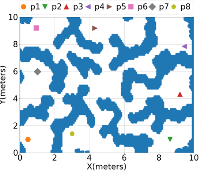
Figure 1: BigGameHunters map base on Starcraft map. Marks represent potential positions from Equations (31-38).

The experiment samples the observations from a simulated model of a common robot with a two-wheeled motor and a one-directional wheel defined by Equation (39), where $\alpha(t)$ is the velocity control and $\omega(t)$ is the angular control rate. $x_{r}(t)$ and $y_{r}(t)$ are the positions in Cartesian axes and $\theta_{r}$ is the orientations in radians. We chose a sampling period of 0.1 seconds and disregarded dynamics such as wheel friction, motor dynamics, and elastic deformations.

$$\footnotesize\dot{x}_{r}(t)=\alpha(t)cos(\theta(t)),$$

$$\dot{y}_{r}(t)=\alpha(t)sin(\theta(t)),$$ (39)

$$\dot{\theta}_{r}(t)=\omega(t).$$

Each recognition problem uses two points to serve as the actual planning problem solved by the robot, with the remaining points being additional goal hypotheses. Thus, we have one problem where the ground truth is a problem from $p_{1}$ to $p_{2}$, with $p_{2}$ to $p_{8}$ being goal hypotheses, another one with $p_{8}$ to $p_{7}$ with $p_{1}$ to $p_{7}$ as goal hypotheses, and so on. This yields 56 goal recognition problems using the Cartesian positions $x$ and $y$ of each point $p_{n}$ from Figure 1.

We assume that the agent pursues a goal with an optimal trajectory regarding some known and computable cost function, i.e., shorter distance, time, and clearance. Specifically, agents optimize total motion time following the dynamical robot model of Equation (39) defined by Equations (40-44), where $\mathit{tf}$ is the total simulation time; $\omega_{lim}$ is the maximal angular velocity; $g_{n}$ is a goal in Cartesian position $x,y$; $W(x_{r}(t),y_{r}(t))$ is a function that measures the Euclidean distance from the robot position to its nearest wall obstacle at time $t$; $W_{lim}$ is the minimum separation between the robot and an obstacle. For our experiments, we define $\omega_{lim}$ to be $3$ rad/s, $g_{n}$ is sampled from Equations (31-38) with free angular orientation, and $W_{lim}$ is $0.01$ meters for all experiments. We represent the complete observation from the initial state $I$ and finish in goal state $g_{n}$ as $O_{I}^{g_{n}}$. Figure 2(a) exemplifies the robot’s optimal trajectory obtained through optimization in the simulated environment. In this example, the robot is pursuing the goal point $g_{2}$ with initial point $p_{1}$ with full observability so that $O_{I}^{g_{n}}={m_{p_{1}}^{g2}}^{*}$.

$${\alpha}^{*},{\omega}^{*}=\operatorname*{argmin}_{\alpha,\,\,\omega}\mathit{tf}$$ (40)

$$subj.\,\,to:\,\,\,\begin{bmatrix}x_{r}(tf)&y_{r}(tf)\end{bmatrix}=g_{n}$$ (41)

$$\lvert\alpha(t)\rvert\leq V_{max},$$ (42)

$$\lvert\omega(t)\rvert\leq\omega_{lim},$$ (43)

$$W(x_{r}(t),y_{r}(t))\geq W_{lim}\,\,\forall\,\,t\in[0,\,\,tf]$$ (44)

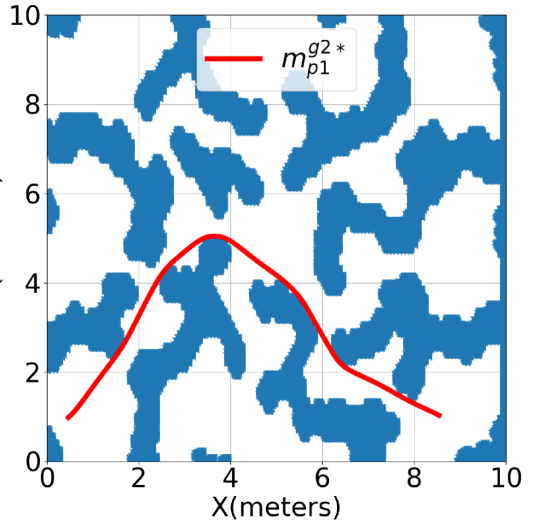
(a) Robot optimal trajectory obtained thought optimization from initial point $p_{1}$ to goal point $g_{2}$.

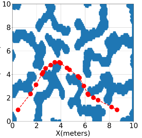
(b) Example of output from ${RRT}^{*}$ considering initial and goal states as $p_{1}$ and $g_{2}$.

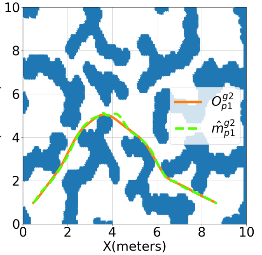
(c) Comparison between the approximated trajectory $\hat{m}_{p_{1}}^{g_{2}}$ and the observation $O_{p_{1}}^{g_{2}}$.

Figure 2: Example of trajectories generated in different stages of the experimental scenario.

4.1 Computing the Via Point Parameters

Figure 3: Convergence example of $J_{\mu}(s)$ Equation (26) in a problem with initial and goal states points as $p_{1}$ and $g_{2}$. The dashed line represents the optimal motion time for this problem.

We use the Open Motion Planning Library (OMPL) [23] with the ${RRT}^{*}$ geometric planning algorithm to compute all the position parameters of Equation (6). This off-the-shelf planner provides a cost-minimal sequence of via point positions from an initial position to a goal. Calls to ${RRT}^{*}$ have a 5-second time limit and use distance as the cost function so that the via points are part of one shortest path to the goal. Figure 2(b) shows an example of an output provided for the ${RRT}^{*}$ planner, where the initial and goal states are $p_{1}$ and $g_{2}$, respectively. Circles are the via points positions provided by the ${RRT}^{*}$ planner, and the dashed line connects them in sequence.

The next stage is finding the velocity parameters of each via point. We implemented a Python version of the optimization previously described in Equations (25-27), which is executed with the SciPy library using the default configuration. The optimization settings are: maximum velocity vector of $V_{max}=1$; random initial actions $\mu$; all acceleration terms in the via points being zero. For example, Figure 3 shows the evolution of the cost function $J_{\mu}(s)$ (in seconds) of Equation (26) throughout the iterations for the problem starting at $p_{1}$ with goal state $g_{2}$. As a reference, we include the optimal motion time for this problem trajectory, obtained from the optimization of Equations (40-44). Note that we expect this difference in motion time since our strategy for trajectory generation uses a polynomial approximation as the robot dynamics model.

Having computed all via points, we use them to compute the approximate trajectory $\hat{m}_{I}^{g}$ from Equation (24). Figure 2(c) shows the trajectory difference between an estimated trajectory $\hat{m}_{p_{1}}^{g_{2}}$ and its respectively observation $O_{p_{1}}^{g_{2}}$. The final stage of our method is to compute the conditional probability of Equation (4) using the estimate trajectories $\hat{m}_{I}^{g_{n}}$ instead of the optimal for each goal at each new observation, allowing us to infer the most likely goal hypotheses. Figure 4 illustrates the conditional probability values $P(\hat{m}_{p_{1}}^{g_{n}}\mid O_{p_{1}}^{g_{2}})$ of Equation (4) for all goals points in the set at each instant in time.

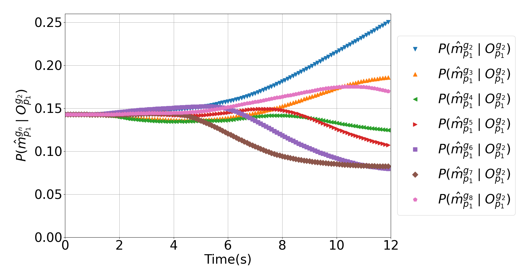
Figure 4: Conditional probabilities $P(\hat{m}_{p_{1}}^{g_{n}}\mid O_{p_{1}}^{g_{2}})$ for all goals in the set in a problem with the initial point at $p_{1}$ and goal point at $g_{2}$.

4.2 Results

We compare our method of online goal recognition with those of Kaminka at al. [9] and Vered at al. [25]. The first approach uses one call to a planner at each new observation and one additional planner call to each goal in the set $G$, totalizing $(|O|+1)|G|$ planner calls. The second approach is similar to the formulation of the first approach but differs by creating a heuristic to decide whether to call a planner at each observation; in practice, the number of calls is between $|G|$ and $(|O|+1)|G|$.

Table 1 compares our method with the Baseline of Kaminka at al. [9] and the Recompute plus Prune (R+P) of Vered at al. [25]. The table shows the positive predictive value (PPV) of the correct goal in percentage and the number of planner calls to get this result for each goal in the set. We group results by problems with the same goal, showing that all goal hypotheses have broadly similar recognition probabilities in most methods. Nevertheless, our approach is less accurate overall, albeit with increased accuracy for some goals.

Table 1: Comparison over 56 problems with eight goals each. PPV. represents the precision in recognizing each goal $g_{n}$, calls report the number of planner calls.

	$\mathbf{Baseline}$		$\mathbf{R+P}$		$\mathbf{Estimation}$
Goal	PPV	Calls	PPV	Calls	PPV	Calls
$g_{1}$	50	343	40.48	225	$\mathbf{52.38}$	$\mathbf{49}$
$g_{2}$	47.62	343	42.86	235	$\mathbf{54.76}$	$\mathbf{49}$
$g_{3}$	$\mathbf{57.14}$	343	54.76	218	45.24	$\mathbf{49}$
$g_{4}$	$\mathbf{59.52}$	343	57.14	193	50	$\mathbf{49}$
$g_{5}$	54.76	343	$\mathbf{76.1}$	205	52.38	$\mathbf{49}$
$g_{6}$	64.29	343	$\mathbf{69.05}$	201	40.48	$\mathbf{49}$
$g_{7}$	$\mathbf{64.29}$	343	57.14	224	57.14	$\mathbf{49}$
$g_{8}$	61.90	343	$\mathbf{73.81}$	199	52.38	$\mathbf{49}$
Avg	57.44	343	$\mathbf{58.93}$	212.15	50.6	$\mathbf{49}$

We divide each of the 56 observable trajectories into six points equally spaced in time, named test observations, to compare the performance of online recognition. Thus, each problem has six sampled points used as observations ($\{o_{1},\dots,o_{6}\}$), which we can use to measure online recognition accuracy (convergence to the correct goal) over time. For example, Figure 5 shows the six sample observations over a complete trajectory with initial and goal states as $p_{1}$ and $g_{2}$. Figure 6 shows the average goal recognition PPV (and its margin of error with a confidence level of 95$\%$) at each of the six sample observations for each method. Results indicate that our method has a similar (error adjusted) accuracy to other methods.

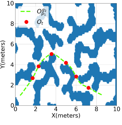
Figure 5: Dashed line represents the full observed trajectory $O_{p_{1}}^{g_{2}}$ and the circles are the test observations sampled to realize the evaluation.

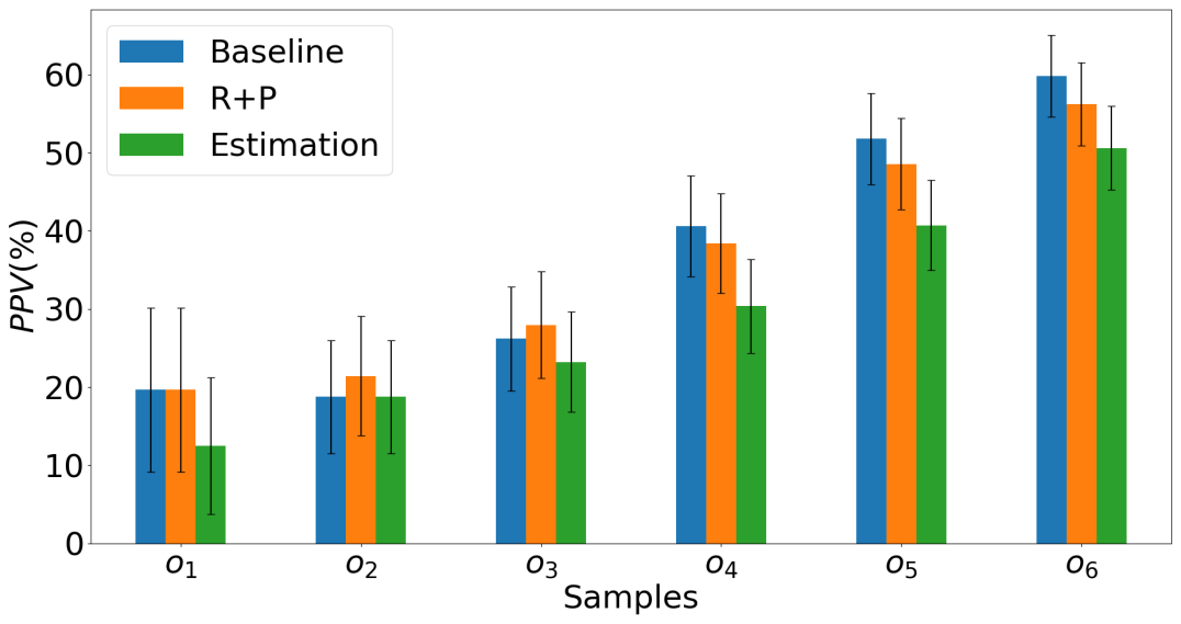
Figure 6: Online accuracy (and error) from different approaches.

Table 2: Run-time comparison (in minutes).

	$\mathbf{Baseline}$	$\mathbf{R+P}$	$\mathbf{Estimation}$
Online run-time	$2889.6$	$1713.48$	$\mathbf{4.62e-4}$
Offline run-time	$481.6$	$513.52$	$\mathbf{123.76}$

Table 2 compares the run-time for three methods of online goal recognition, separating the online and offline parts of the algorithm. This table shows the critical advantage of our method: while the offline computations have a fourfold speed up, the online computations improve by seven orders of magnitude.

5 Discrete Domains

Table 3: Comparison among online goal recognition methods for discrete domains.

				Online Mirroring					Online Mirroring with Landmarks					Vector Inference
	$|\mathcal{O}|$	$|\mathcal{G}|$	$|$S$|$	PPV	ACC	SPR	T	PC	PPV	ACC	SPR	T	PC	PPV	ACC	SPR	T	PC
FERRY	18.83	6.33	1.00	0.59	0.87	1.75	16.95	126.08	0.54	0.85	1.75	13.80	98.41	0.65	0.90	1.59	0.68	6.33
DRIVERLOG	12.16	6.66	1.00	0.66	0.89	1.69	17.47	86.16	0.66	0.89	1.65	7.55	48.66	0.69	0.90	1.68	1.03	6.66
MICONIC	16.33	6.00	1.00	0.59	0.87	1.77	17.38	104.00	0.38	0.77	1.68	9.57	80.75	0.67	0.89	1.63	0.74	6.00
IPC-GRID	11.87	7.50	1.00	0.58	0.86	2.04	19.07	100.00	0.48	0.82	2.07	17.12	91.12	0.59	0.86	2.03	1.27	7.50
ROVERS	10.83	6.00	1.00	0.57	0.86	1.79	70.92	71.00	0.39	0.78	1.77	56.21	56.00	0.74	0.93	1.41	13.13	6.00
ZENO	12.00	6.00	1.00	0.63	0.89	1.62	20.23	78.00	0.53	0.85	1.55	15.32	40.75	0.68	0.90	1.58	3.39	6.00

Our approach from Section 3 works exclusively for an online goal recognition formulate in a vectorial representation (continuous domain). At first glance, it may not seem trivial to directly apply it to discrete domains, which comprise the largest goal recognition datasets openly available [16]. However, to apply the inference developed in this work, we develop a conversion of the discrete state into a vectorial continuous state space representation, allowing us to apply our recognition approach.

We consider a discrete domain to be a STRIPS-style PDDL description with the same semantics of Fikes et al. [5] as $\mathcal{D}$, with typed objects set $Z$ and a set of typed predicates $\mathcal{R}$. A classical planning problem can be described as $\mathcal{P}=\langle\mathcal{F},\mathcal{A},\mathcal{I},\mathcal{G}\rangle$, where: $\mathcal{F}$ is the set of facts (instantiated predicates from Z); $\mathcal{A}$ is the set actions with objects from $Z$; $\mathcal{I}\in\mathcal{F}$ is the initial state; and $\mathcal{G}\subseteq\mathcal{F}$ is the goal state. A discrete goal recognition problem is a tuple $\mathcal{L}=\langle\mathcal{D},\mathcal{O},\mathcal{I},\mathcal{G}\rangle$, where: $\mathcal{D}$ is the domain defined above; $\mathcal{O}\subseteq\mathcal{F}$ is a set of observations. A trajectory in a discrete domain is a sequence of ordered states (represented by a set of fluents $\mathcal{F}$), while a plan $\pi$ is a sequence of ordered actions (represented by possible actions $\mathcal{A}$ of the domain). Plans here match exactly their definition from classical planning [7].

Algorithm 1 describes the online goal recognition process. In an offline stage of the inference, a classical planner solves the problem $\mathcal{P}$ for each goal hypothesis to compute a plan $\pi_{n}$ (Line 4). Then, we roll out the resulting plan to generate intermediary states (Line 5). The states computed in the previous step are converted to a vectorial continuous state space using the function described in Algorithm 2 (Lines 6-7). Line 8 constitutes the run-time goal inference at each new observation, which consists of converting the symbolic observations to vector form (Line 10) and computing the conditional probability of each goal following the Bayesian formulation of goal recognition. The rank function (Line 11) is a direct computation of Equation (3) for each goal hypothesis.

Algorithm 2 requires as input the set of predicates $\mathcal{R}$, the set of objects $Z$, and the state $S$ to be converted. At the end of the conversion process, the algorithm provides a vector with a length of $|\mathcal{R}|\times|Z|$, where each position represents the occurrence frequency of a conjugate predicate and object in the current time step $k$.

Algorithm 1 Discrete Online Goal Recognition in Vector Representation

1:$\mathcal{P}=\langle\mathcal{F},\mathcal{A},\mathcal{I},\mathcal{G}\rangle$, $\mathcal{R}$, $Z$

2:function onlineVectorInference($\mathcal{P},\mathcal{R},Z$)

3:     for $\textbf{all}\,{g_{n}}\in\mathcal{G}$ do $\triangleright$ Offline precomputation of optimal plans

4:         $\pi_{n}\leftarrow\textsc{Planner}(\mathcal{P},g_{n})$

5:         $states\leftarrow rollout(\mathcal{P},\pi_{n})$

6:         for $\textbf{all}\,S\in states$ do

7:              $m_{I}^{g_{n}}.append(\textsc{STRIPStoVec}(\mathcal{R},Z,S))$                

8:     while $New\,o_{k}\in\mathcal{O}$ is available do $\triangleright$ Online recognition

9:         for $\textbf{all}\,g_{n}\in\mathcal{G}$ do

10:              $\mathcal{O}_{v}\leftarrow\{\textsc{STRIPStoVec}(\mathcal{R},Z,o)\mid o\in\mathcal{O}\}$

11:              $P(\mathcal{O}\mid m_{I}^{g_{n}})\leftarrow\textsc{rank}(\mathcal{O}_{v},m_{I}^{g_{n}})$               

Algorithm 2 STRIPS to Vectorial Continuous Domain

1:function STRIPStoVec($\mathcal{R},Z,S$)

2:     $v[|\mathcal{R})|*|Z|]\leftarrow 0$

3:     $i\leftarrow 0$

4:     for $\textbf{all}\,predicate\in\mathcal{R}$ do

5:         for $\textbf{all}\,object\in Z$ do

6:              for $\textbf{all}\,s\in S$ do

7:                  if $predicate,\,object\subseteq s$ then

8:                       $v[i]\leftarrow v[i]+1$                                 

9:              $i\leftarrow i+1$               

10:     $\textbf{return}\,v$

6 Experiments in Discrete Domains

We evaluate our inference method empirically against two online goal recognition methods. The first method is Mirroring by Kaminka at al. [9], which we use as a Baseline. The second method is an extension of the baseline approach, Mirroring with Landmarks by Vered at al. [26], which is the current state-of-the-art. Our experiments use an openly available goal and plan recognition dataset [16]. This dataset contains thousands of recognition problems comprising large and non-trivial planning problems (with optimal and sub-optimal plans as observations) for 15 planning domains, including domains and problems from datasets from Ramírez at al. [20]. All planning domains in these datasets use the STRIPS fragment of the Planning Domain Definition Language (PDDL). Domains include realistic applications (e.g., DWR, ROVERS, LOGISTICS), and hard artificial domains (e.g., SOKOBAN). Each problem in these datasets contains a complete domain definition, an initial state, a set of candidate goals, and a correct hidden goal in the set of candidate goals.

Table 3 shows the result of our empirical evaluation of these methods against our online goal recognition formulation for discrete domains, All results are averages over 12 problems for each experiment domain. The table includes the following information: $|\mathcal{O}|$ is the observation set size, which represents the whole plan that achieves the hidden goal, i.e., having observed 100% of the actions; $|\mathcal{G}|$ is the goal hypothesis set size; $|S|$ is the solution set size; positive predictive value (PPV); overall accuracy (ACC) for each experiment; spread (SPR) is the size of the hypothesis solution set chosen by recognition method; (T) is the sum of online and offline time, and (PC) is the number of planner calls during the whole recognition process. Figure 7 compares results among the methods at four points during observation (and its margin of error with a confidence level of 95$\%$), at $30\%$, $50\%$, $70\%$, and $100\%$ of their respective full observation. All results shown in the Figure 7 are averages over the problems of each experiment domain. For example, partial observation problems ($30\%$, $50\%$, and $70\%$) have an average of 36 problems for each domain, and the full observation has an average length of 12 actions. We generate observations and optimal plans using the Fast Downward planner running $A^{*}$ with the LM-cut heuristic. Results indicate that our approach is faster across the board, using substantially fewer calls to the planner than all other approaches. Importantly, our approach provides superior accuracy (substantially so in some domains) and PPV, with a marginally higher spread in only two domains.

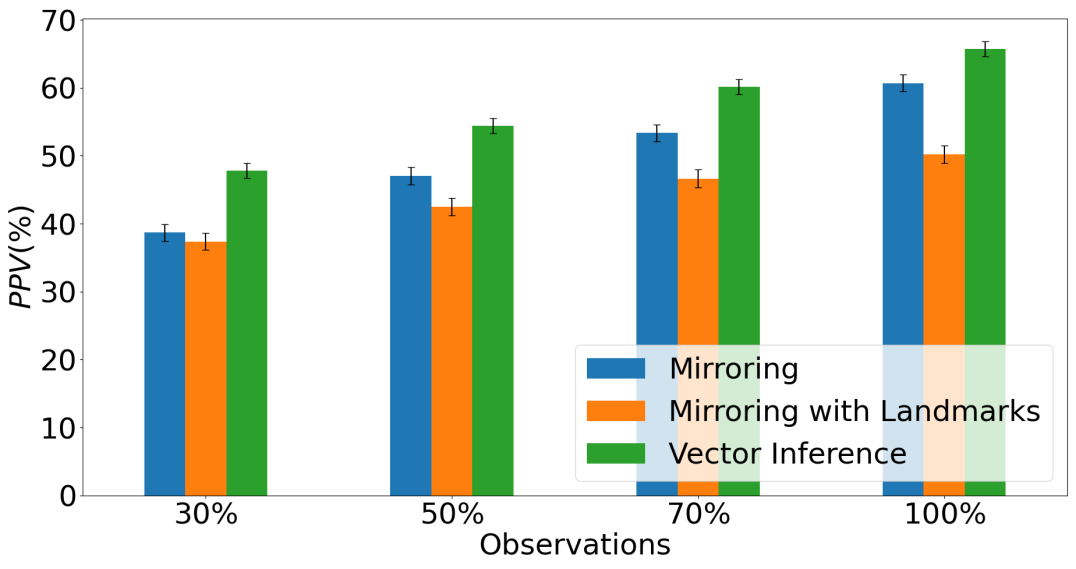
Figure 7: PPV percent and margin of error from different approaches over observation percentages.

7 Conclusion

This paper introduces an online goal recognition approach suitable for continuous and discrete domains. Our approach is suitable for recognition of agent motion in continuous environments with obstacles. If we know the observed agent’s initial states and a set of possible goals a priori, almost all computations can be executed in an offline stage. At each new observation, a simple equation executes the inference process in milliseconds providing the probability distribution over the goals. We develop a mechanism for discrete domains to convert STRIPS-style problems into vectors amenable to our function approximation.

Our evaluation shows that our method needs fewer planner calls than other methods while yielding comparable, and often superior, recognition results. Our method is seven orders of magnitude faster than the state-of-the-art and four times faster than the state-of-the-art in the preprocessing stage. This advantage in execution time is due to our method using a smaller number of fixed planner calls ($|G|$), replacing most of the original planner calls by an approximate model of motion. By contrast, the baseline uses a much larger fixed number of planner calls of $(|O|+1)|G|$, and the R+P method have a variable number of planner calls between $|G|$ and $(|O|+1)|G|$. While our approach is slower than the fastest approaches for discrete domains [16], it is the only approach with similar runtime characteristics that works for continuous and discrete domains.

Empirical results showcase the difference between computing an optimal trajectory and using an approximated one. Computing an optimal trajectory is often a complex task for any continuous domain optimization; using an approximation naturally reduces the overall optimization complexity. The major drawback of using an approximation is a reduction in accuracy. However, we argue that the orders of magnitude speed-up we obtain more than compensates for the penalty imposed on accuracy. Specifically, any method that takes minutes to perform online goal recognition in a moving robot is impractical. The variance shows similarities among the methods, which indicates that the developed method has a similar density probability but is bias-polarized by the estimation. Finally, our goal recognition method for continuous domains sets us up to a new class of goal recognition methods suitable for applications where recognition must happen in milliseconds (e.g., for robots in motion).

References

- [1] Dimitri Bertsekas, Reinforcement learning and optimal control, Athena Scientific, 2019.
- [2] Howie Choset, Kevin M Lynch, Seth Hutchinson, George A Kantor, and Wolfram Burgard, Principles of robot motion: theory, algorithms, and implementations, MIT press, 2005.
- [3] John J Craig, Introduction to robotics: mechanics and control, Pearson Educacion, 2005.
- [4] Andrew Dobson and Kostas E Bekris, ‘Sparse roadmap spanners for asymptotically near-optimal motion planning’, The International Journal of Robotics Research, 33(1), 18–47, (2014).
- [5] Richard E Fikes and Nils J Nilsson, ‘Strips: A new approach to the application of theorem proving to problem solving’, Artificial intelligence, 2(3-4), 189–208, (1971).
- [6] Jonathan D Gammell, Timothy D Barfoot, and Siddhartha S Srinivasa, ‘Batch informed trees (bit*): Informed asymptotically optimal anytime search’, The International Journal of Robotics Research, 39(5), 543–567, (2020).
- [7] Malik Ghallab, Dana S. Nau, and Paolo Traverso, Automated planning - theory and practice, Elsevier.
- [8] Avik Jain, Lawrence Chan, Daniel S Brown, and Anca D Dragan, ‘Optimal cost design for model predictive control’, in Learning for Dynamics and Control, pp. 1205–1217. PMLR, (2021).
- [9] Gal A Kaminka, Mor Vered, and Noa Agmon, ‘Plan recognition in continuous domains’, in Thirty-Second AAAI Conference on Artificial Intelligence, (2018).
- [10] Sertac Karaman and Emilio Frazzoli, ‘Sampling-based algorithms for optimal motion planning’, The international journal of robotics research, 30(7), 846–894, (2011).
- [11] Kevin M Lynch and Frank C Park, Modern Robotics: Mechanics, Planning, and Control, Cambridge University Press, 2017.
- [12] Peta Masters and Sebastian Sardina, ‘Cost-based goal recognition for path-planning’, in Proceedings of the 16th Conference on Autonomous Agents and MultiAgent Systems, pp. 750–758, (2017).
- [13] Felipe Meneguzzi and Ramon F. Pereira, ‘A survey on goal recognition as planning’, in Thirtieth AAAI Conference on Artificial Intelligence, (2021).
- [14] Reuth Mirsky, Sarah Keren, and Christopher Geib, ‘Introduction to symbolic plan and goal recognition’, Synthesis Lectures on Artificial Intelligence and Machine Learning, 16(1), 1–190, (2021).
- [15] Saeed B Niku, Introduction to robotics: analysis, control, applications, John Wiley & Sons, 2020.
- [16] Ramon Pereira, Nir Oren, and Felipe Meneguzzi, ‘Landmark-based heuristics for goal recognition’, in Proceedings of the AAAI Conference on Artificial Intelligence, volume 31, (2017).
- [17] Ramon Pereira, Nir Oren, and Felipe Meneguzzi, ‘Landmark-based approaches for goal recognition as planning’, Artificial Intelligence, 279, 103217, (12 2019).
- [18] Mihail Pivtoraiko, Ross A Knepper, and Alonzo Kelly, ‘Differentially constrained mobile robot motion planning in state lattices’, Journal of Field Robotics, 26(3), 308–333, (2009).
- [19] Miguel Ramírez and Hector Geffner, ‘Probabilistic plan recognition using off-the-shelf classical planners’, in Twenty-Fourth AAAI Conference on Artificial Intelligence, (2010).
- [20] Miquel Ramírez and Hector Geffner, ‘Plan recognition as planning’, in Twenty-First AAAI Conference on Artificial Intelligence, (2009).
- [21] Wilko Schwarting, Javier Alonso-Mora, and Daniela Rus, ‘Planning and decision-making for autonomous vehicles’, Annual Review of Control, Robotics, and Autonomous Systems, 1(1), 187–210, (2018).
- [22] Nathan R Sturtevant, ‘Benchmarks for grid-based pathfinding’, IEEE Transactions on Computational Intelligence and AI in Games, 4(2), 144–148, (2012).
- [23] Ioan A. Şucan, Mark Moll, and Lydia E. Kavraki, ‘The Open Motion Planning Library’, IEEE Robotics & Automation Magazine, 19(4), 72–82, (December 2012). https://ompl.kavrakilab.org.
- [24] Gita Sukthankar, Christopher Geib, Hung Hai Bui, David Pynadath, and Robert P Goldman, Plan, activity, and intent recognition: Theory and practice, Elsevier, 2014.
- [25] Mor Vered and Gal A Kaminka, ‘Heuristic online goal recognition in continuous domains’, in Twenty-Sixth AAAI Conference on Artificial Intelligence, pp. 4447–4454, (2017).
- [26] Mor Vered, Ramon Fraga Pereira, Gal Kaminka, and Felipe Rech Meneguzzi, ‘Towards online goal recognition combining goal mirroring and landmarks’, in Proceedings of the 17th International Conference on Autonomous Agents and MultiAgent Systems, p. 10–15, (2018).
- [27] Yu Zhang, Sarath Sreedharan, Anagha Kulkarni, Tathagata Chakraborti, Hankz Hankui Zhuo, and Subbarao Kambhampati, ‘Plan explicability and predictability for robot task planning’, in 2017 IEEE International Conference on Robotics and Automation (ICRA), pp. 1313–1320, (2017).