RegExplainer: Generating Explanations for Graph Neural Networks in Regression Task

Abstract.

Graph regression is a fundamental task that has gained significant attention in various graph learning tasks. However, the inference process is often not easily interpretable. Current explanation techniques are limited to understanding GNN behaviors in classification tasks, leaving an explanation gap for graph regression models. In this work, we propose a novel explanation method to interpret the graph regression models (XAIG-R). Our method addresses the distribution shifting problem and continuously ordered decision boundary issues that hinder existing methods away from being applied in regression tasks. We introduce a novel objective based on the information bottleneck theory and a new mix-up framework, which could support various GNNs in a model-agnostic manner. Additionally, we present a contrastive learning strategy to tackle the continuously ordered labels in regression tasks. We evaluate our proposed method on three benchmark datasets and a real-life dataset introduced by us, and extensive experiments demonstrate its effectiveness in interpreting GNN models in regression tasks.

1. Introduction

Graph Neural Networks (Scarselli et al., 2009) (GNNs) have become a powerful tool for learning knowledge from graph-structure data (Henaff et al., 2015) and achieved remarkable performance in many areas, including social networks (Fan et al., 2019; Min et al., 2021), molecular structures (Chereda et al., 2019; Mansimov et al., 2019), traffic flows (Wang et al., 2020; Li and Zhu, 2021; Wu et al., 2019; Yu et al., 2018), recommendation systems (Shaikh et al., 2017; Wu et al., 2022b; Yang and Toni, 2018), and knowledge graphs (Sorokin and Gurevych, 2018). The capability of GNNs from its propagating and message-passing mechanisms(Scarselli et al., 2009), which are fusing messages from neighboring nodes on the graph, helps GNNs achieve state-of-the-art performance in many tasks like node classification (Xiao et al., 2022), graph classification (Lee et al., 2018; Zhang et al., 2018), graph regression (Jia and Benson, 2020; Zhao et al., 2019), link prediction (Zhang and Chen, 2018; Cai et al., 2021), etc. However, despite their success, people still lack an understanding of how GNNs make predictions. This lack of explainability is becoming a more important topic, as understanding how GNNs make predictions can increase user confidence when using GNNs in high-stakes applications (Yuan et al., 2022; Longa et al., 2022), enhance the transparency of the models, and make them suitable for use in sensitive fields such as healthcare and drug discovery (Xiong et al., 2019; Bongini et al., 2021), where fairness, privacy, and safety are critical concerns(Zhang et al., 2022; Wu et al., 2022a; Li et al., 2022). Therefore, exploring the interpretability of GNNs is essential.

One way to enhance the transparency of GNN models is by using post-hoc instance-level explainability methods. These methods aim to explain the predictions made by trained GNN models by identifying key sub-graphs in input graphs. Examples of such methods include GNNExplainer (Ying et al., 2019), which determines the importance of nodes and edges through perturbation, and PGExplainer (Luo et al., 2020), which trains a graph generator to incorporate global information. Recent studies (Yuan et al., 2021; Shan et al., 2021a) have contributed to the development of these methods. Post-hoc explainability methods fall under a label-preserving framework, where the explanation is a sub-graph of the original graph and preserves the information about the predicted label. On top of the intuitive principle, Graph Information Bottleneck (GIB) (Wu et al., 2020; Miao et al., 2022; Yu et al., 2020) maximizes the mutual information $I(G^{*};Y)$ between the target label $Y$ and the explanation $G^{*}$ while constraining the size of the explanation as the mutual information between the original graph $G$ and the explanation $G^{*}$.

However, all the methods mentioned above are focusing on the explanation of the graph classification task (Lee et al., 2018; Xiao et al., 2022; Zhang et al., 2018). To the best of our knowledge, none of the existing work has investigated the explanation of the graph regression task. The graph regression tasks exist widely in nowadays applications, such as predicting the molecular property (Brockschmidt, 2020) or traffic flow volume (Rusek et al., 2022). Therefore, it’s crucial to provide high-quality explanations for the graph regression task.

Explaining the instance-level results of graph regression in a post-hoc manner is challenging due to two main obstacles: 1. the GIB objective in previous work is not applicable in the regression task; 2. the distribution shifting problem (Wiles et al., 2021; Fang et al., 2020; Hendrycks and Gimpel, 2016; Zhang et al., 2023).

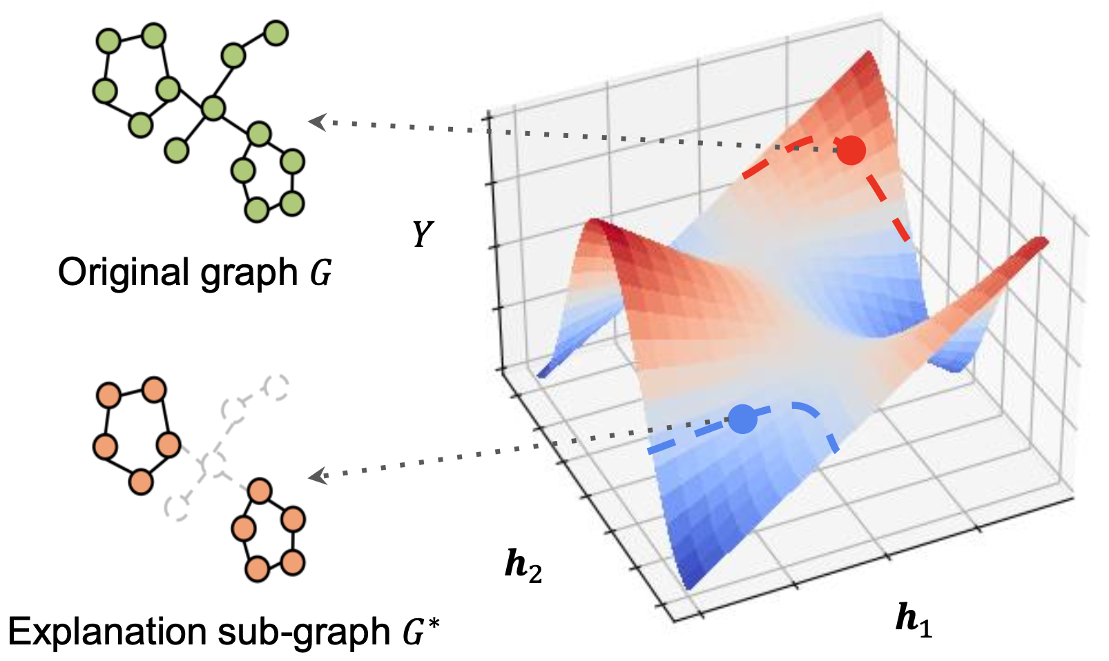
Figure 1. Intuitive illustration of the distribution shifting problem. The 3-dimensional map represents a trained GNN model $f$, where $(h_{1},h_{2})$ represents the distribution of the graph in two dimensions, and $Y$ represents the prediction value of the graph through $f$. The red and blue lines represent the distribution of the original training set and corresponding explanation sub-graph set respectively.

$\bullet$ One challenge is the mutual information estimation in the GIB objective. In previous works (Ying et al., 2019; Luo et al., 2020; Miao et al., 2022) for graph classification, the mutual information $I(G^{*};Y)$ is estimated with the Cross-Entropy between the the predictions $f(G^{*})$ from GNN model $f$ and its prediction label $Y$ from the original graph $G$. However, in the regression task, the regression label is the continuous value, instead of categorized classes, making it difficult to be estimated with the cross entropy loss. Therefore, we adopt the GIB objective to employ the InfoNCE objective and contrastive loss to address this challenge and estimate the mutual information.

$\bullet$ Another challenge is the distribution shifting problem, which means the explanation sub-graphs are out-of-distribution(OOD) of the original training graph dataset. As shown in Figure 1, a GNN model is trained on the original graph training set for a graph regression task. The previous work always assumes that the explanation sub-graph would contain the same mutual information as the original graph ideally. However, as seen in the figure, even when $G$ and $G^{*}$ both have two motifs as the label information, $f(G^{*})$ is different from $f(G)$ due to a different distribution. Due to the explanation sub-graph usually having a different topology and feature information compare to the original graph, the GNN model trained on the original graph set couldn’t accurately predict with the explanation sub-graph, which means we couldn’t directly estimate the mutual information between the original graph and the explanation sub-graph due to the distribution shifting problem.

In this paper, for the first time, we propose RegExplainer, to generate post-hoc instance-level explanations for graph regression tasks. Specifically, to address the distribution shifting issue, RegExplainer develops a mix-up approach to generate the explanation from a sub-graph into the mix-up graph without involving the label-preserving information. To capture the continuous targets in the regression task, RegExplainer also adopts the GIB objective to utilize the contrastive loss to learn the relationships between the triplets $[G,G^{+},G^{-}]$ of the graphs, where $G$ is the target to-be-explained graph and $G^{+}$ and $G^{-}$ are positive and negative instances respectively. Our experiments show that RegExplainer provides consistent and concise explanations of GNN’s predictions on regression tasks. We achieved up to $86.3\%$ improvement when compared to the alternative baselines in our experiments. Our contributions could be summarized as in the following:

• To our best knowledge, we are the first to explain the graph regression tasks. We addressed two challenges associated with the explainability of the graph regression task: the mutual information estimation in the GIB objective and the distribution shifting problem.

• We proposed a novel model with a new mix-up approach and contrastive learning, which could more effectively address the two challenges, and better explain the graph model on the regression tasks compared to other baselines.

• We designed three synthetic datasets, namely BA-regression, BA-counting, and Triangles, as well as a real-world dataset called Crippen, which could also be used in future works, to evaluate the effectiveness of our regression task explanations. Comprehensive empirical studies on both synthetic and real-world datasets demonstrate that our method can provide consistent and concise explanations for graph regression tasks.

2. Preliminary

2.1. Notation and Problem Formulation

We use $G=(\mathcal{V},\mathcal{E};{\bm{X}},{\bm{A}})$ to represent a graph, where ${\mathcal{V}}$ equals to $\{{v}_{1},{v}_{2},...,{v}_{n}\}$ represents a set of $n$ nodes and $\mathcal{E}\in\mathcal{V}\times\mathcal{V}$ represents the edge set. Each graph has a feature matrix ${\bm{X}}\in\mathbb{R}^{n\times d}$ for the nodes, wherein ${\bm{X}}$, ${X}_{i}\in\mathbb{R}^{1\times d}$ is the $d$-dimensional node feature of node $v_{i}$. $\mathcal{E}$ is described by an adjacency matrix ${\bm{A}}\in\{0,1\}^{n\times n}$, where ${A}_{ij}=1$ means that there is an edge between node $v_{i}$ and $v_{j}$; otherwise, ${A}_{ij}=0$. For the graph prediction task, each graph $G_{i}$ has a label $Y_{i}\in{\mathcal{C}}$, where ${\mathcal{C}}$ is the set of the classification categories or regression values, with a GNN model $f$ trained to make the prediction, i.e., $f:({\bm{X}},{\bm{A}})\mapsto{\mathcal{C}}$.

Problem 1 (Post-hoc Instance-level GNN Explanation).

Given a trained GNN model $f$, for an arbitrary input graph $G=(\mathcal{V},\mathcal{E};{\bm{X}},{\bm{A}})$, the goal of posthoc instance-level GNN explanation is to find a sub-graph $G^{*}$ that can explain the prediction of $f$ on $G$.

In non-graph structured data, the informative feature selection has been well studied (Li et al., 2017), as well as in traditional methods, such as concrete auto-encoder (Balın et al., 2019), which can be directly extended to explain features in GNNs. In this paper, we focus on discovering the important sub-graph typologies following the previous work (Ying et al., 2019; Luo et al., 2020). Formally, the obtained explanation $G^{*}$ is depicted by a binary mask ${\bm{M}}^{*}\in\{0,1\}^{n\times n}$ on the adjacency matrix, e.g., $G^{*}=(\mathcal{V},\mathcal{E};{\bm{X}},{\bm{A}}\odot{\bm{M}}^{*})$, $\odot$ means elements-wise multiplication. The mask highlights components of $G$ which are essential for $f$ to make the prediction.

2.2. GIB Objective

The Information Bottleneck (IB) (Tishby et al., 2000; Tishby and Zaslavsky, 2015) provides an intuitive principle for learning dense representations that an optimal representation should contain minimal and sufficient information for the downstream prediction task. Based on IB, a recent work unifies the most existing post-hoc explanation methods for GNN, such as GNNExplainer (Ying et al., 2019), PGExplainer (Luo et al., 2020), with the graph information bottleneck (GIB) principle (Wu et al., 2020; Miao et al., 2022; Yu et al., 2020). Formally, the objective of explaining the prediction of $f$ on $G$ can be represented by

(1) $$\operatorname*{arg\,min}_{G^{*}}I(G;G^{*})-\alpha I(G^{*};Y),$$

where $G$ is the to-be-explained original graph, $G^{*}$ is the explanation sub-graph of $G$, $Y$ is the original ground-truth label of $G$, and $\alpha$ is a hyper-parameter to get the trade-off between minimal and sufficient constraints. GIB uses the mutual information $I(G;G^{*})$ to select the minimal explanation that inherits only the most indicative information from $G$ to predict the label $Y$ by maximizing $I(G^{*};Y)$, where $I(G;G^{*})$ avoids imposing potentially biased constraints, such as the size or the connectivity of the selected sub-graphs (Wu et al., 2020). Through the optimization of the sub-graph, $G^{*}$ provides model interpretation.

In graph classification task, a widely-adopted approximation to Eq. (2) in previous methods is:

(2) $$\operatorname*{arg\,min}_{G^{*}}I(G;G^{*})+\alpha I(Y|G^{*})\approx\operatorname*{arg\,min}_{G^{*}}I(G;G^{*})+\alpha\text{CE}(Y,Y^{*}),$$

where $Y^{*}=f(G^{*})$ is the predicted label of $G^{*}$ made by the model to be explained, $f$ and the cross-entropy $\text{CE}(Y,Y^{*})$ between the ground truth label $Y$ and $Y^{*}$ is used to approximate $I(G^{*};Y)$. The approximation is based on the definition of mutual information $I(G^{*};Y)=H(Y)-H(Y|G^{*})$: with the entropy $H(Y)$ being static and independent of the explanation process, minimizing the mutual information between the explanation sub-graph $G^{*}$ and $Y$ can be reformulated as maximizing the conditional entropy of $Y$ given $G^{*}$, which can be approximated by the cross-entropy between $Y$ and $Y^{*}$.

3. Methodology

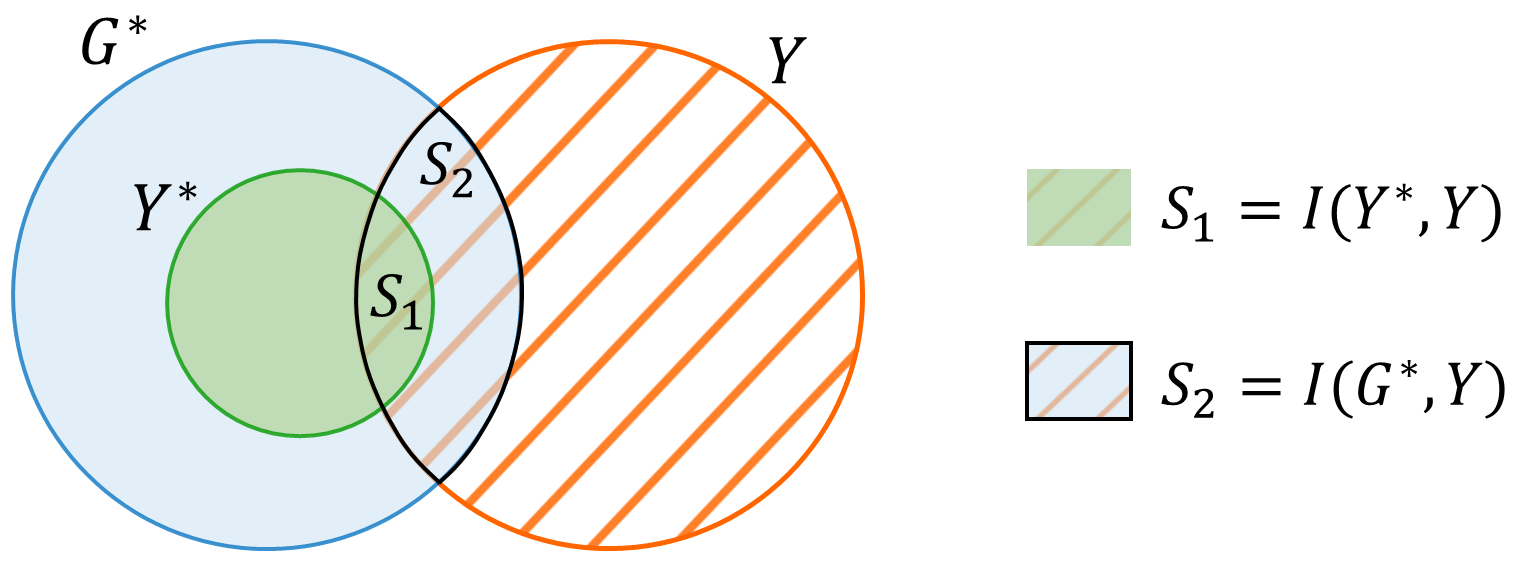
Figure 2. Intuitive illustration about why $I(G^{*};Y)\geq I(Y^{*};Y)$. $G^{*}$ contains more mutual information as more overlapping area with $Y$ than the overlapping between $Y^{*}$ and $Y$.

In this section, we first introduce a new objective based on GIB for explaining graph regression learning. Then we showcase the distribution shifting problem in the GIB objective in graph regression tasks and propose a novel framework through a mix-up approach to solve the shifting problem.

3.1. GIB for Explaining Graph Regression

As introduced in Section 2.2, in the classification task, $I(G^{*};Y)$ in Eq. (1) is commonly approximated by cross-entropy $\text{CE}(Y^{*},Y)$ (Zhang and Sabuncu, 2018). However, it is non-trivial to extend exiting objectives for regression tasks because $Y$ is a continuous variable and makes it intractable to compute the cross-entropy $\text{CE}(Y^{*},Y)$ or the mutual information $I(G^{*};Y)$, where $G^{*}$ is a graph variable with a continuous variable $Y^{*}$ as its label.

3.1.1. Optimizing the lower bound of $I(G^{*};Y)$

To address the challenge of computing the mutual information $I(G^{*};Y)$ with a continuous $Y$, we propose a novel objective for explaining graph regression. Instead of minimizing $I(G^{*};Y)$ directly, we propose to maximize a lower bound for the mutual information by including the label of $G^{*}$, denoted by $Y^{*}$, and approximate $I(G^{*};Y)$ with $I(Y^{*};Y)$, where $Y^{*}$ is the prediction label of $G^{*}$:

(3) $$\operatorname*{arg\,min}_{G^{*}}I(G;G^{*})-\alpha I(Y^{*};Y).$$

As shown below, $I(Y^{*};Y)$ has the following property:

Property 1. $I(Y^{*};Y)$ is a lower bound of $I(G^{*};Y)$.

Proof.

From the definition of $Y^{*}$, we can make a safe assumption that there is a many-to-one map (function), denoted by $h$, from $G^{*}$ to $Y^{*}$ as $Y^{*}$ is the prediction label for $G^{*}$. For simplicity, we assume a finite number of explanation instances for each label $y^{*}$, and each explanation instance, denoted by $g^{*}$, is generated independently. Then, we have $p(y^{*})=\sum_{g^{*}\in{\mathbb{G}}(y^{*})}p(g^{*})$, where ${\mathbb{G}}(y^{*})=\{g|h(g)=y^{*}\}$ is the set of explanations whose labels are $y^{*}$.

Based on the definition of mutual information, we have:

$$I(G^{*};Y)=\int_{y}\int_{g^{*}}p_{(G^{*},Y)}(g^{*},y)\log\frac{p_{(G^{*},Y)}(g^{*},y)}{p_{G^{*}}(g^{*})p_{Y}(y)}d_{g^{*}}d_{y}$$

$$=\int_{y}\int_{g^{*}}p_{(G^{*},Y^{*},Y)}(g^{*},h(g^{*}),y)\log\frac{p_{(G^{*},Y^{*},Y)}(g^{*},h(g^{*}),y)}{p_{G^{*}}(g^{*})p_{Y}(y)}d_{g^{*}}d_{y}$$

$$=\int_{y}\int_{g^{*}}p_{(G^{*},Y^{*},Y)}(g^{*},h(g^{*}),y)\log\frac{p_{(G^{*},Y^{*},Y)}(g^{*},h(g^{*}),y)}{p_{(G^{*},Y^{*})}(g^{*},h(g^{*}))p_{Y}(y)}d_{g^{*}}d_{y}$$

$$=\int_{y}\int_{y^{*}}\sum_{g^{*}\in{\mathbb{G}}(y^{*})}p_{(G^{*},Y^{*},Y)}(g^{*},y^{*},y)\log\frac{p_{(G^{*},Y^{*},Y)}(g^{*},y^{*},y)}{p_{(G^{*},Y^{*})}(g^{*},y^{*})p_{Y}(y)}d_{y^{*}}d_{y}$$

Based on our many-to-one assumption , while each $g^{*}$ is generated independently , we know that if $g\notin{\mathbb{G}}(y^{*})$, then $p_{(G^{*},Y^{*},Y)}(g^{*},y^{*},y)=0$. Thus, we have:

$$I(G^{*};Y)=I(G^{*};Y)$$

$$+\int_{y}\int_{y^{*}}\sum_{g\notin{\mathbb{G}}(y^{*})}p_{(G^{*},Y^{*},Y)}(g^{*},y^{*},y)\log\frac{p_{(G^{*},Y^{*},Y)}(g^{*},y^{*},y)}{p_{(G^{*},Y^{*})}(g^{*},y^{*})p_{Y}(y)}d_{y^{*}}d_{y}$$

$$=\int_{y}\int_{y^{*}}\int_{g*}p_{(G^{*},Y^{*},Y)}(g^{*},y^{*},y)\log\frac{p_{(G^{*},Y^{*},Y)}(g^{*},y^{*},y)}{p_{(G^{*},Y^{*})}(g^{*},y^{*})p_{Y}(y)}d_{g^{*}}d_{y^{*}}d_{y}$$

$$=I(G^{*},Y^{*};Y).$$

With the chain rule for mutual information, we have $I(G^{*},Y^{*};Y)=I(Y^{*};Y)+I(G^{*};Y|Y^{*})$. Then due to the non-negativity of the mutual information, we have $I(G^{*},Y^{*};Y)\geq I(Y^{*};Y)$. ∎

Intuitively, the property of $I(Y^{*};Y)$ is guaranteed by the chain rule for mutual information and the independence between each explanation instance $g^{*}$. The intuitive demonstration is shown in Figure 2. With the property, we can approximate Eq. (1) with Eq. (3).

3.1.2. Estimating $I(Y^{*};Y)$ with InfoNCE

Now the challenge becomes the estimation of the mutual information $I(Y^{*};Y)$. Inspired by the model of Contrastive Predictive Coding (van den Oord et al., 2019), in which InfoNCE loss is interpreted as a mutual information estimator, we further extend the method so that it could apply to InfoNCE loss in explaining graph regression.

In our graph explanation scenario, $I(Y^{*};Y)$ has the following property:

Property 2. InfoNCE Loss is a lower bound of the $I(Y^{*};Y)$ as shown in Eq. (4).

(4) $$I(Y^{*};Y)\geq\underset{\mathbb{Y}}{\mathbb{E}}\left[\log\frac{f_{k}\left(Y^{*},Y\right)}{\frac{1}{|\mathbb{Y}|}\sum_{Y_{j}\in\mathbb{Y}}f_{k}\left(Y^{*},Y_{j}\right)}\right]$$

In Eq. (4), $Y_{j}$ is randomly sampled graph neighbors, and $\mathbb{Y}$ is the set of the neighbors. We prove this property theoretically in the following:

Proof.

As in the InfoNCE method, the mutual information between $Y^{*}$ and $Y$ is defined as:

(5) $$I(Y^{*};Y)=\sum_{Y^{*},Y}p(Y^{*},Y)\log\frac{p(Y|Y^{*})}{P(Y)}$$

However, the ground truth joint distribution $p(Y^{*},Y)$ is not controllable, so, we turn to maximize the density ratio

(6) $$f_{k}\left(Y^{*},Y\right)\propto\frac{p(Y|Y^{*})}{p(Y)}$$

We want to put the representation function of mutual information into the NCE Loss

(7) $$\mathcal{L}_{N}=-\underset{\mathbb{Y}}{\mathbb{E}}\log\left[\frac{f_{k}\left(Y^{*},Y\right)}{\sum_{Y^{\prime}\in\mathbb{Y}}(Y^{*},Y^{\prime})}\right],$$

where $\mathcal{L}_{N}$ denotes the NCE loss and by inserting the optimal $f_{k}\left(Y^{*},Y\right)$ into Eq. (7), we could get:

(8) $$\begin{split}\mathcal{L}_{\text{contr}}&=-\underset{\mathbb{Y}}{\mathbb{E}}\log\left[\frac{\frac{p(Y|Y^{*})}{p(Y)}}{\frac{p(Y|Y^{*})}{p(Y)}+\sum_{Y^{\prime}\in\mathbb{Y}_{\text{neg}}}\frac{p(Y^{*},Y^{\prime})}{p(Y^{\prime})}}\right]\\ &=\underset{\mathbb{Y}}{\mathbb{E}}\log\left[1+\frac{p(Y|Y^{*})}{p(Y)}\sum_{Y^{\prime}\in\mathbb{Y}_{\text{neg}}}\frac{p(Y^{*},Y^{\prime})}{p(Y^{\prime})}\right]\\ &\thickapprox\underset{\mathbb{Y}}{\mathbb{E}}\log\left[1+\frac{p(Y|Y^{*})}{p(Y)}(N-1)\underset{Y^{\prime}}{\mathbb{E}}\frac{p(Y^{*},Y^{\prime})}{p(Y^{\prime})}\right]\\ &=\underset{\mathbb{Y}}{\mathbb{E}}\log\left[1+\frac{p(Y|Y^{*})}{p(Y)}(N-1)\right]\\ &\geq\underset{\mathbb{Y}}{\mathbb{E}}\log\left[\frac{p(Y|Y^{*})}{p(Y)}N\right]\\ &=-I(Y^{*},Y)+\log(N)\end{split}$$

∎

To employ the contrastive loss, we use the representation embedding to approximate $Y$, where ${\bm{h}}^{*}$ represents the embedding for $G^{*}$ and ${\bm{h}}$ represents the embedding for $G$. We use $\mathbb{H}$ to represent the neighbors set $\mathbb{Y}$ accordingly. Thus, we approximate Eq. (3) as:

(9) $$\operatorname*{arg\,min}_{G^{*}}I(G;G^{*})-\alpha\underset{\mathbb{H}}{\mathbb{E}}\left[\log\frac{f_{k}\left({\bm{h}}^{*},{\bm{h}}\right)}{\frac{1}{|\mathbb{H}|}\sum_{{\bm{h}}_{j}\in\mathbb{H}}f_{k}\left({\bm{h}}^{*},{\bm{h}}_{j}\right)}\right]$$

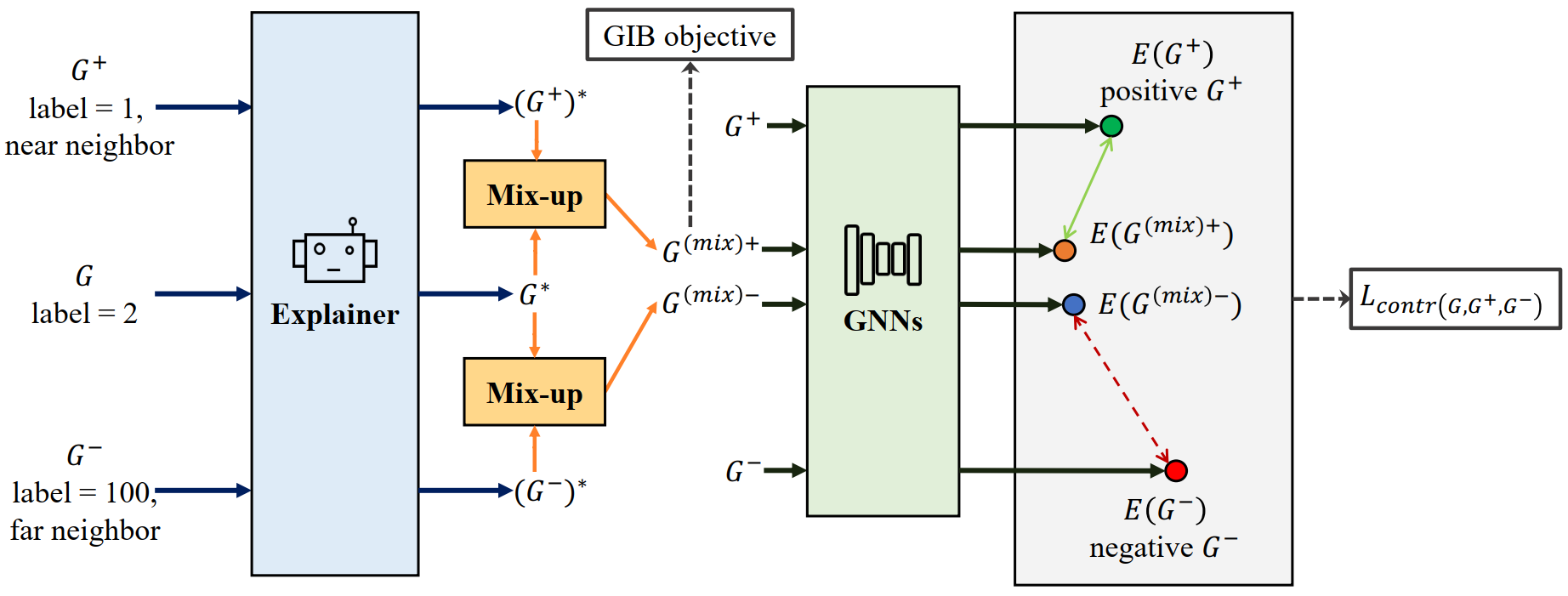
Figure 3. Illustration of RegExplainer. $G$ is the to-be-explained graph, $G^{+}$ is the randomly sampled positive graph and $G^{-}$ is the randomly sampled negative graph. The explanation of the graph is produced by the explainer model. Then graph $G$ is mixed with $G^{+}$ and $G^{-}$ respectively to produce $G^{\text{(mix)}+}$ and $G^{\text{(mix)}-}$. Then the graphs are fed into the trained GNN model to retrieve the embedding vectors $E(G^{+})$, $E(G^{-})$, $E(G^{\text{(mix)}-})$ and $E(G^{\text{(mix)}-})$. We use contrastive loss to minimize the distance between $G^{\text{(mix)}+}$ and the positive sample and maximum the distance between $G^{\text{(mix)}-}$ and the negative sample. The explainer is trained with the GIB objective and contrastive loss.

3.2. Mixup for Distribution Shifts

In the above section, we include the label of explanation sub-graph, $Y^{*}$, in our GIB objective for explaining regression. However, we argue that $Y^{*}$ cannot be safely obtained due to the distribution shift problem (Fang et al., 2023a; Zhang et al., 2023).

3.2.1. Distribution Shifts in GIB

Suppose that the model to be explained, $f$, is trained on a dataset $\{(G_{i},Y_{i})\}_{i=1}^{N}$. Usually in supervised learning (without domain adaptation), we suppose that the examples $(G_{i},Y_{i})$ are drawn i.i.d. from a distribution ${\mathcal{D}}_{\text{train}}$ of support $G\times Y$ (unknown and fixed). The objective is then to learn $f$ such that it commits the least error possible for labeling new examples coming from the distribution ${\mathcal{D}}_{\text{train}}$. However, as pointed out in previous studies, there is a shift between the distribution explanation sub-graphs, denoted by ${\mathcal{D}}_{\text{exp}}$ and ${\mathcal{D}}_{\text{train}}$. As the explanation, sub-graphs tend to be small and dense. The distribution shift problem is severe in regression problems due to the continuous decision boundary (Liu et al., 2021).

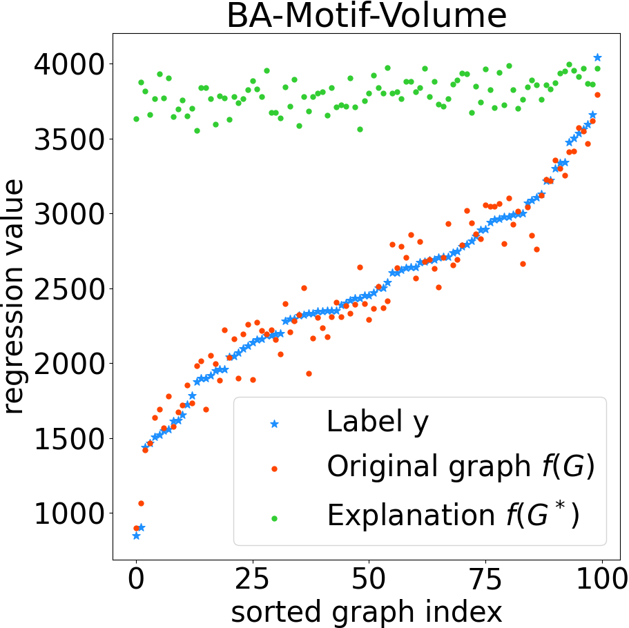
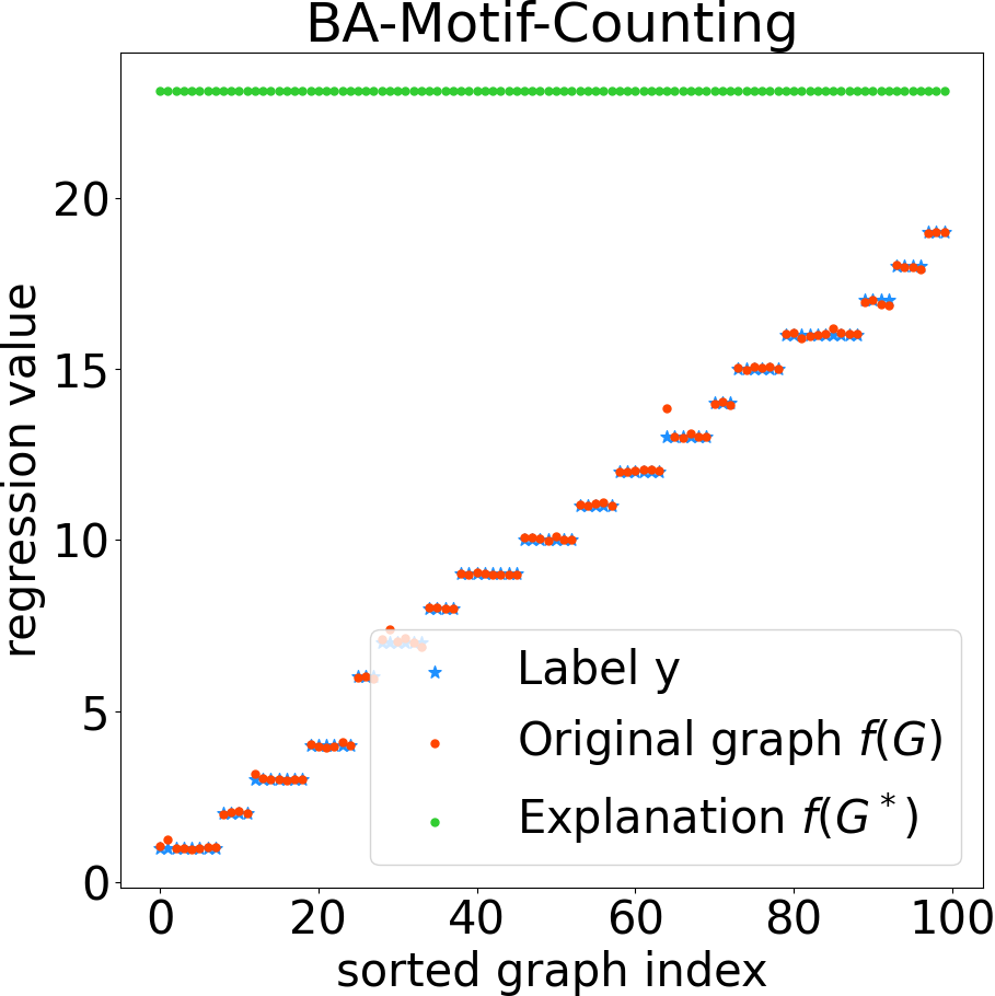
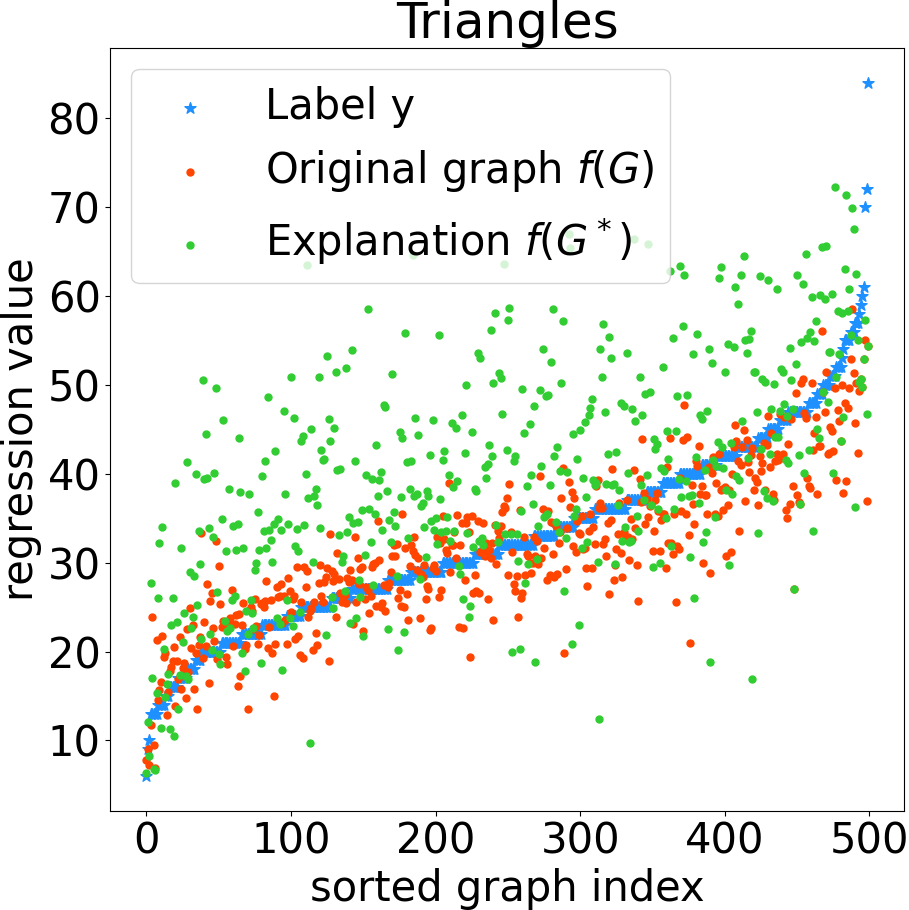
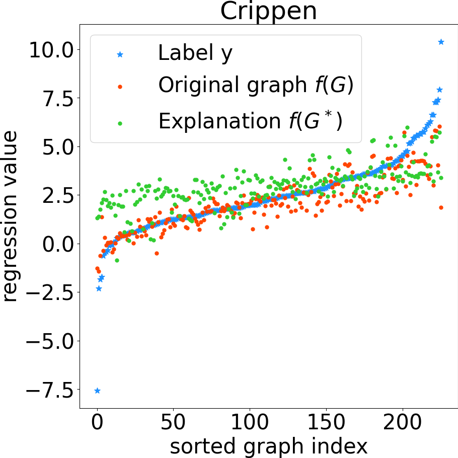
Figure 4. Visualization of distribution shifting problem on four graph regression datasets. The points represent the regression value, where the blue points mean label $y$, red points mean prediction $f(G)$ of the original graph, and the blue points mean prediction $f(G^{*})$ of explanations on the four datasets, the x-axis is the indices of the graph, sorted by the value of the label $Y$.

Figure 4 shows the existence of distribution shifts between $f(G^{*})$ and $Y$ in graph regression tasks. For each dataset, we sort the indices of the data samples according to the value of their labels, and visualize the label $Y$, prediction $f(G)$ of the original graph from the trained GNN model $f$, and prediction $f(G^{*})$ of the explanation sub-graph $G^{*}$ from $f$. As we can see in Figure 3, in all four graph regression datasets, the red points are well distributed around the ground-truth blue points, indicating that $f(G)$ is close to $Y$. In comparison, the green points shift away from the red points, indicating the shifts between $f(G^{*})$ and $f(G)$. Intuitively, this phenomenon indicates the GNN model $f$ could make correct predictions only with the original graph $G$ yet could not predict the explanation sub-graph $G^{*}$ correctly. This is because the GNN model $f$ is trained with the original graph sets, whereas the explanation $G^{*}$ as the sub-graph is out of the distribution from the original graph sets. With the shift between $f(G)$ and $f(G^{*})$, the optimal solution in Eq. (3) is unlikely to be the optimal solution for Eq. (1).

3.2.2. Graph Mix-up Approach.

To address the distribution shifting issue between $f(G)$ and $f(G^{*})$ in the GIB objective, we introduce the mix-up approach to reconstruct a within-distribution graph, $G^{\text{(mix)}}$, from the explanation graph $G^{*}$. We follow (Luo et al., 2020) to make a widely-accepted assumption that a graph can be divided by $G=G^{*}+G^{\Delta}$, where $G^{*}$ presents the underlying sub-graph that makes important contributions to GNN’s predictions, which is the expected explanatory graph, and $G^{\Delta}$ consists of the remaining label-independent edges for predictions made by the GNN. Both $G^{*}$ and $G^{\Delta}$ influence the distribution of $G$. Therefore, we need a graph $G^{\text{(mix)}}$ that contains both $G^{*}$ and $G^{\Delta}$, upon which we use the prediction of $G^{\text{(mix)}}$ made by $f$ to approximate $Y^{*}$ and ${\bm{h}}^{*}$.

Specifically, for a target graph $G_{a}$ in the original graph set to be explained, we generate the explanation sub-graph $G_{a}^{*}=G_{a}-G_{a}^{\Delta}$ from the explainer. To generate a graph in the same distribution of original $G_{a}$, we can randomly sample a graph $G_{b}$ from the original set, generate the explanation sub-graph of $G_{b}^{*}$ with the same explainer and retrieve its label-irrelevant graph $G_{b}^{\Delta}=G_{b}-G_{b}^{*}$. Then we could merge $G_{a}^{*}$ together with $G_{b}^{\Delta}$ and produce the mix-up explanation $G_{a}^{\text{(mix)}}$. Formally, we can have $G_{a}^{\text{(mix)}}=G_{a}^{*}+(G_{b}-G_{b}^{*})$.

Since we are using the edge weights mask to describe the explanation, the formulation could be further written as:

(10) $${\bm{M}}_{a}^{\text{(mix)}}={\bm{M}}_{a}^{*}+({\bm{I}}_{b}-{\bm{M}}_{b}^{*}),$$

where ${\bm{M}}$ denotes the weight of the adjacency matrix and ${\bm{I}}_{b}$ denotes the zero-ones matrix as weights of all edges in the adjacency matrix of $G_{b}$, where 1 represents the existing edge and 0 represents there is no edge between the node pair.

We denote $G_{a}$ and $G_{b}$ with the adjacency matrices $A_{a}$ and $A_{b}$, their edge weight mask matrices as $M_{a}$ and $M_{b}$. If $G_{a}$ and $G_{b}$ are aligned graphs with the same number of nodes, we could simply mix them up with Eq. (10). However, in real-life applications, a well-aligned dataset is rare. So we use a connection adjacency matrix $A_{\text{conn}}$ and mask matrix $M_{\text{conn}}$ to merge two graphs with different numbers of nodes. Specifically, the mix-up adjacency matrix could be formed as:

(11) $${\bm{A}}_{a}^{\text{(mix)}}=\left[\begin{array}[]{cc}{\bm{A}}_{a}&{\bm{A}}_{\text{conn}}\\ {\bm{A}}^{T}_{\text{conn}}&{\bm{A}}_{b}\end{array}\right].$$

And the mix-up mask matrix could be formed as:

(12) $${\bm{M}}^{(\text{mix})}_{a}=\left[\begin{array}[]{cc}{\bm{M}}_{a}^{*}&{\bm{M}}_{\text{conn}}\\ {\bm{M}}^{T}_{\text{conn}}&{\bm{M}}_{b}^{\Delta}\end{array}\right]$$

Finally, we could form $G_{a}^{\text{(mix)}}$ as $({\bm{X}}^{\text{(mix)}},{\bm{A}}_{a}^{\text{(mix)}}\odot{\bm{M}}_{a}^{\text{(mix)}})$, where ${\bm{X}}^{\text{(mix)}}=[{\bm{X}}_{a};{\bm{X}}_{b}]$. We use Algorithm 1 to describe the whole process. Then we could feed $G_{a}^{\text{(mix)}}$ into the GIB objective and use it for training the parameterized explainer.

Algorithm 1 Graph Mix-up Algorithm

1:Target to-be-explained graph $G_{a}=({\bm{X}}_{a},{\bm{A}}_{a})$, $G_{b}$ sampled from a set of graphs $\mathbb{G}$, the number of random connections $\eta$, explainer model $E$.

2:Graph $G^{\text{(mix)}}$.

3:Generate mask matrix ${\bm{M}}_{a}=E(G_{a})$

4:Generate mask matrix ${\bm{M}}_{b}=E(G_{b})$

5:Sample $\eta$ random connections between $G_{a}$ and $G_{b}$ as ${\bm{A}}_{\text{conn}}$

6:Mix-up adjacency matrix ${\bm{A}}_{a}^{\text{(mix)}}$ with Eq. (11)

7:Mix-up edge mask ${\bm{M}}_{a}^{\text{(mix)}}$ with Eq. (12)

8:Mix-up node features ${\bm{X}}^{\text{(mix)}}=[{\bm{X}}_{a};{\bm{X}}_{b}]$

9:return $G^{\text{(mix)}}=({\bm{X}}^{\text{(mix)}},{\bm{A}}_{a}^{\text{(mix)}}\odot{\bm{M}}_{a}^{\text{(mix)}})$

We show that our mix-up approach has the following property: Property 3. $G^{\text{(mix)}}$ is within the distribution of ${\mathcal{D}}_{\text{train}}$.

Proof.

Following the previous work, we denote a graph $G=G^{*}+G^{\Delta}$, where $G^{*}$ is the sub-graph explanation and $G^{\Delta}$ is the label-irrelevant graph. A common acknowledgment is that for a graph $G$ with label $Y$, the explanation $G^{*}$ holds the label-preserving information, which is the important sub-graph, while $G^{\Delta}$ also holds useful information which makes sure connecting it with $G^{*}$ would maintain the distribution of the graph and not lead to another label. We denote the distribution for the graphs as $G\sim{\mathcal{D}}_{\text{train}}=\mathbb{P}_{\mathcal{G}}$, $G^{*}\sim\mathbb{P}_{\mathcal{G}^{*}}$, $G^{\Delta}\sim\mathbb{P}_{\mathcal{G}^{\Delta}}$, where ${\mathcal{D}}_{\text{train}}$ means the distribution of train dataset. When we produce $G^{\text{(mix)}}$, we independently sample a label-irrelevant graph $G^{\Delta}$ and mix it up with target explanation $G^{*}$. So, we could write the distribution of $G^{\text{(mix)}}$ as :

(13) $$G^{\text{(mix)}}\sim\mathbb{P}_{\mathcal{G}^{*}}*\mathbb{P}_{\mathcal{G}^{\Delta}}=\mathbb{P}_{(\mathcal{G}^{*}+\mathcal{G}^{\Delta})}=\mathbb{P}_{\mathcal{G}}={\mathcal{D}}_{\text{train}}$$

Thus, we prove that $G^{\text{(mix)}}$ is within the distribution of ${\mathcal{D}}_{\text{train}}$. ∎

3.3. Implementation

3.3.1. Implementation of InfoNCE Loss.

After generating the mix-up explanation $G^{\text{(mix)}}$, we specify the contrastive loss to further train the parameterized explainer with a triplet of graphs $(G,G^{+},G^{-})$ as the implementation of InfoNCE Loss in Eq. (9). Intuitively, for each target graph $G$ with label $Y$ to be explained, we can define two randomly sampled graphs as positive graph $G^{+}$ and negative instance $G^{-}$ where $G^{+}$’s label, $Y^{+}$ is closer to $Y$ than $G^{-}$’s label, $Y^{-}$, i.e., $|Y^{+}-Y|<|Y^{-}-Y|$. Therefore, the distance between the distributions of the positive pair $(G,G^{+})$ should be smaller than the distance between the distributions of the negative pair $(G,G^{-})$.

In practice, $G^{+}$ and $G^{-}$ are randomly sampled from the graph dataset, upon which we calculate their similarity score with the target graph $G$. The sample with a higher score would be the positive sample and the other one would be the negative sample. Specifically, we use $\text{sim}({\bm{h}},{\bm{h}}_{j})={\bm{h}}^{T}{\bm{h}}_{j}$ to compute the similarity score, where $G_{j}$ could be $G^{+}$ or $G^{-}$. ${\bm{h}}$ is generated by feeding $G$ into the GNN model $f$ and directly retrieving the embedding vector before the dense layers ; ${\bm{h}}^{+}$ and ${\bm{h}}^{-}$ denote the embedding vectors for $G^{+}$ and $G^{-}$ respectively.

Learning through the triplet instances could effectively reinforce the ability of the explainer to learn the explanation self-supervised. A similar idea goes with mixup graphs which we propose to address the distribution shifts in GIB. After we mix up target graph $G$ with the neighbors $G^{+}$ and $G^{-}$ and get $G^{\text{(mix)}+}$ and $G^{\text{(mix)}-}$ respectively, the distance between $G^{\text{(mix)}+}$, $G^{+}$ should be smaller than the distance between $G^{\text{(mix)}-}$, $G^{-}$. For example, given graph $G$ with a label $2.0$, $G^{+}$ with a label $1.0$, and $G^{-}$ with a label $100.0$, after we mix the explanation of $G$, which is $G^{*}$, with $G^{+}$ and $G^{-}$ respectively, following Eq. (10), the prediction label of $G^{\text{(mix)}+}$ and $G^{\text{(mix)}-}$ should be closer to $1$ because they contain the label-preserving sub-graph $G^{*}$, which could be represented as $|f(G^{\text{(mix)}-})-f(G^{-})|>|f(G^{\text{(mix)}+})-f(G^{+})|$, where $f(G)$ represents the prediction label of graph $G$.

Formally, given a target graph $G$, the sampled positive graph $G^{+}$ and negative graph $G^{-}$, we formulate the contrastive loss in Eq. (9) as the following:

(14) $$\begin{split}\mathcal{L}_{\text{contr}}(G,G^{+},G^{-})&=\log(1+\exp({\bm{h}}^{T}{\bm{h}}^{-}-{\bm{h}}^{T}{\bm{h}}^{+}))\\ &=-\log\frac{\exp({\bm{h}}^{T}{\bm{h}}^{+})}{\exp({\bm{h}}^{T}{\bm{h}}^{+})+\exp({\bm{h}}^{T}{\bm{h}}^{-})}\end{split}$$

where $\exp()$ function is used to instantiate the density ratio function $f_{k}$, the denominator is a sum over the ratios of both positive and negative samples in the triplet $\mathbb{Y}$.

Algorithm 2 Training Explainer

1:A set of graphs $\mathbb{G}$, trained GNN model $f$, explainer model $E$.

2:Trained explainer $E$.

3:Initialize explainer model $E$.

4:for $e\in epochs$ do

5:     for $G\in\mathbb{G}$ do

6:         $G_{b},G_{c}\leftarrow$ Randomly sample two graphs from $\mathbb{G}$

7:         $G^{+},G^{-}\leftarrow$ Compare similarity$(G_{b},G_{c})$ to $G$

8:         $G^{\text{(mix)}+}\leftarrow$ Mix-up $(G,G^{+})$ with Algorithm 1

9:         $G^{\text{(mix)}-}\leftarrow$ Mix-up $(G,G^{-})$ with Algorithm 1

10:         Computing $\mathcal{L}_{\text{contr}}(G,G^{+},G^{-})$ with Eq. (14)

11:         Computing $\mathcal{L}_{\text{GIB}}$ with Eq. (16)

12:         Computing overall loss $\mathcal{L}$ with Eq. (17)

13:     end for

14:     Update $E$ with back propagation.

15:end for

16:return Explainer $E$

3.3.2. Size Constraints

We optimize $I(G;G^{*})$ in Eq. (9) to constraint the size of the explanation sub-graph $G^{*}$. The upper bound of $I(G;G^{*})$ is optimized as the estimation of the KL-divergence between the probabilistic distribution between the $G^{*}$ and $G$, where the KL-divergence term can be divided into two parts as the entropy loss and size loss (Miao et al., 2022). In practice, we follow the previous work (Ying et al., 2019; Luo et al., 2020; Xie et al., 2022) to implement them. Specifically,

(15) $$\mathcal{L}_{\text{size}}(G,G^{*})=\gamma\underset{(i,j)\in\mathcal{E}}{\sum}({M}^{*}_{ij})-\log\delta({\bm{h}}{\bm{h}}^{T}).$$

$\underset{(i,j)\in\mathcal{E}}{\sum}({M}^{*}_{ij})$ means sum the weights of the existing edges in the edge weight mask ${\bm{M}}^{*}$ for the explanation $G^{*}$; ${\bm{h}}=f_{\text{ebd}}(G^{*})$, where we extract the embedding of the graph $G^{*}$ before the GNN model $f$ transforming it into prediction $Y^{*}$ and $\gamma$ is the weight for the size of the masked graph.

3.3.3. Overall Objective Function.

In practice, the denominator in Eq. (9) works as a regularization to avoid trivial solutions. Since the label $Y=f(G)$ is given and independent of the optimization process, we could also employ the MSE loss between $Y^{*}$ and $Y$ additionally, regarding InfoNCE loss only estimates the mutual information between the embeddings. Formally, the overall loss function could be implemented as:

(16) $$\mathcal{L}_{\text{GIB}}=\mathcal{L}_{\text{size}}(G,G^{*})-\alpha\mathcal{L}_{\text{contr}}(G,G^{+},G^{-})$$

(17) $$\begin{split}\mathcal{L}=\mathcal{L}_{\text{GIB}}+\beta\mathcal{L}_{\text{MSE}}(f(G),f(G^{\text{(mix)}+})),\end{split}$$

where $G^{\text{(mix)}+}$ means mix $G^{*}$ with the positive sample $G^{+}$ and the hyper-parameters are $\alpha$ and $\beta$.

3.3.4. Detailed Description of Algorithm 2

Algorithm 2 shows the training phase for the explainer model $E$. For each epoch and each to-be-explained graph, we first randomly sample two neighbors $G_{b}$ and $G_{c}$, then we decide the positive sample $G^{+}$ and negative sample $G^{-}$ according to the similarity between $(G,G_{b})$ and $(G,G_{c})$. We generate the explanation for graphs and mix $G$ with $G^{+}$ and $G^{-}$ respectively with the Algorithm 1. We calculate the contrastive loss for triplet $(G,G^{+},G^{-})$ with Eq.( 14) and the GIB loss, which contains the size loss and contrastive loss. We also calculate the MSE loss between $f(G^{\text{(mix)}+})$ and $f(G)$. The overall loss is the sum of GIB loss and MSE loss. We update the trainable parameters in the explainer with the overall loss.

3.3.5. Computational Complexity Analysis

In the implementation, we transform the structure of the graph data from the sparse adjacency matrix representation into the dense edges list representation. We analyze the computational complexity of our mix-up approach here. According to Algorithm 1, given a graph $G_{a}$ and a randomly sampled graph $G_{b}$, assuming $G_{a}$ contains $M_{a}$ edges and $G_{b}$ contains $M_{b}$ edges, the complexity of graph extension operation on edge indices and masks, which extend the size of them from $M_{a}$, $M_{b}$ to $M_{a}+M_{b}$, is $\O(2(M_{a}+M_{b}))$, where $M_{a}>0$ and $M_{b}>0$. To generate $\eta$ cross-graph edges, the computational complexity is ${\mathcal{O}}(\eta)$. For the mix-up operation, the complexity is ${\mathcal{O}}(2(M_{a}+M_{b})+\eta)$. Since $\eta$ is usually a small constant, the time complexity of our mix-up approach is ${\mathcal{O}}(2*M_{a}+2*M_{b})$. We use $M$ to denote the largest number of edges for the graph in the dataset and the time complexity of mix-up could be simplified to ${\mathcal{O}}(M)$.

4. Experiments

Table 1. Illustration of the graph regression dataset together with the explanation faithfulness in terms of AUC-ROC on edges under four datasets on RegExplainer and other baselines. The original graph row visualize the structure of the complete graph, the explanation row highlight the explanation sub-graph of the corresponding original graph. In Crippen dataset, different color of the node represent different kind of atoms and the node feature is one-hot vector to encode the atom type.

Dataset	BA-Motif-Volume	BA-Motif-Counting	Triangles	Crippen
Original Graph $G$
Explanation $G^{*}$
Node Feature	Random Float Vector	Fixed Ones Vector	Fixed Ones Vector	One-hop Vector
Regression Label	Sum of Motif Value	Count Motifs	Count Triangles	Chemical Property Value
Explanation Type	Fix Size Sub-Graph	Dynamic Size Sub-graph	Dynamic Size Sub-graph	Dynamic Size Sub-graph
Explanation AUC
GRAD	$0.418\pm 0.000$	$0.516\pm 0.000$	$0.479\pm 0.000$	$0.426\pm 0.000$
ATT	$0.512\pm 0.005$	$0.517\pm 0.003$	$0.441\pm 0.004$	$0.502\pm 0.006$
GNNExplainer	$0.501\pm 0.009$	$0.496\pm 0.003$	$0.500\pm 0.002$	$0.497\pm 0.005$
PGExplainer	$0.470\pm 0.057$	$0.000\pm 1.56$	$0.511\pm 0.028$	$0.448\pm 0.005$
RegExplainer	$\mathbf{0.758\pm 0.177}$	$\mathbf{0.963\pm 0.011}$	$\mathbf{0.739\pm 0.008}$	$\mathbf{0.553\pm 0.013}$

In this section, we will introduce our datasets, experiment settings, and the results. Our experiments show that RegExplainer provides consistent and concise explanations of GNN’s predictions on regression tasks. On three synthetic datasets and real-life dataset Crippen, we show that RegExplainer accurately identifies the important sub-graphs/motifs that determine the graph label and outperforms alternative baselines by up to $86.3\%$ in explanation accuracy (AUC).

• RQ1: How does the RegExplainer perform compared to other baselines on the four datasets?

• RQ2: How does each component of the proposed approach affect the performance of RegExplainer?

• RQ3: How does the proposed approach perform under different hyper-parameters?

4.1. Datasets and Setups

In this section, we will introduce how we formulate our datasets and their specific configurations. (1) BA-Motif-Volume: This dataset is based on the BA-shapes (Ying et al., 2019) and makes a modification, which is adding random float values from [0.00, 100.00] as the node feature. We then sum the node values on the motif as the regression label of the whole graph, which means the GNNs should recognize the [house] motif and then sum features to make the prediction. (2) BA-Motif-Counting: Different from BA-Motif-Volume, where node features are summarized, in this dataset, we attach various numbers of motifs to the base BA random graph and pad all graphs to equal size. The number of motifs is counted as the regression label. Padding graphs to the same size could prevent the GNNs from making trivial predictions based on the total number of nodes. (3) Triangles: We follow the previous work (Chen et al., 2020) to construct this dataset. The dataset is a set of $5000$ Erdős–Rényi random graphs denoted as $ER(m,p)$, where $m=30$ is the number of nodes in each graph and $p=0.2$ is the probability for an edge to exist. The size of $5000$ was chosen to match the previous work. The regression label for this dataset is the number of triangles in a graph and GNNs are trained to count the triangles. (4) Crippen: The Crippen dataset is a real-life dataset that was initially used to evaluate the graph regression task. The dataset has 1127 graphs reported in the Delaney solubility dataset (Delaney, 2004) and has weights of each node assigned by the Crippen model (Wildman and Crippen, 1999), which is an empirical chemistry model predicting the water-actual partition coefficient. We adopt this dataset, firstly shown in the previous work (Sanchez-Lengeling et al., 2020), and construct edge weights by taking the average of the two connected nodes’ weights. The regression label is the water-actual partition coefficient of the molecule graph.

4.1.1. Baselines

We compared the proposed RegExplainer against a comprehensive set of baselines in all datasets, including: (1) GRAD  (Ying et al., 2019): GRAD is a gradient-based method that learns weight vectors of edges by computing gradients of the GNN’s objective function. (2) ATT  (Veličković et al., 2017): ATT is a graph attention network (GAT) that learns attention weights for edges in the input graph. These weights can be utilized as a proxy measure of edge importance. (3) GNNExplainer (Ying et al., 2019): GNNExplainer is a model-agnostic method that learns an adjacency matrix mask by maximizing the mutual information between the predictions of the GNN and the distribution of possible sub-graph structures. (4) PGExplainer (Luo et al., 2020): PGExplainer adopts a deep neural network to parameterize the generation process of explanations, which facilitates a comprehensive understanding of the predictions made by GNNs. It also produces sub-graph explanations with edge importance masks.

4.2. Quantitative Evaluation (RQ1)

In this section, we aim to answer RQ1 by evaluating the performance of our approach and comparing it to other baselines. For GRAD and GAT, we use the gradient-based and attention-based explanation, following the setting in the previous work  (Ying et al., 2019). For GNNExplainer and PGExplainer, which are previously used for the classification task, we replace the Cross-Entropy loss with the MSE loss. We run and tune all the baselines on our four datasets. We evaluate the explanation from all the methods with the AUC metric, as done in the previous work. As we can see in the table, our method achieves the best performance compared to the baselines in all four datasets.

As shown in Table 1, we qualitatively study the explaining performance of RegExplainer and other baselines. We note that in Table 1, the original graphs and explanation sub-graphs we put in rows 1&2 for four datasets are sketch maps, which may not accurately depict the number of nodes and edges in the graphs but rather provide insight into the nature of the graphs in the dataset. As we can observe in the table, RegExplainer improves the second baseline with 0.246/48.4% on average and up to 0.446/0.863%. The comparison between RegExplainer and other baselines indicates the advantages of our purposed approach.

4.3. Ablation Study (RQ2)

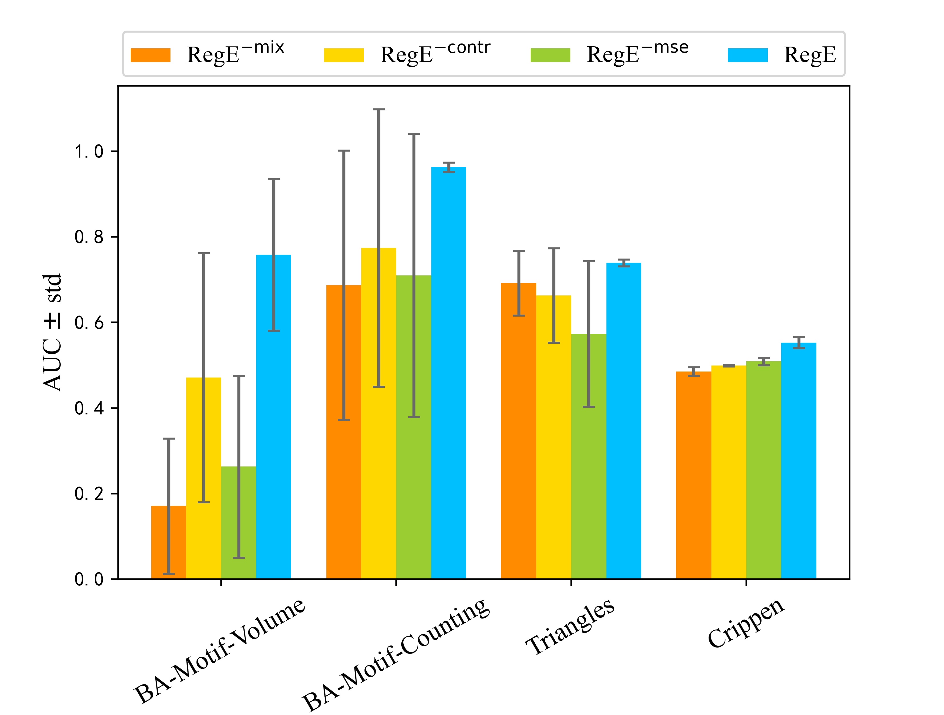
Figure 5. Ablation study of RegExplainer. We evaluated the performance of original RegExplainer and its variants that exclude mix-up approach, contrastive loss, or MSE loss respectively. The X-axis indicates the various datasets, while the bars represent the AUC score, and the black solid line shows the standard deviation value.

To answer RQ2, we conducted an ablation study to show how our proposed components, specifically, the mix-up approach and contrastive learning, contribute to the final performance of RegExplainer. To this end, we denote RegExplainer as RegE and design three types of variants as follows: (1) $\text{RegE}^{-\text{mix}}$: We remove the mix-up processing after generating the explanations and feed the sub-graph $G^{*}$ into GIB objective and contrastive loss directly. (2) $\text{RegE}^{-\text{contr}}$: We directly remove the contrastive loss term but still maintain the mix-up processing and MSE loss. (3) $\text{RegE}^{-\text{mse}}$: We directly remove the MSE loss computation item from the objective function.

Additionally, we set all variants with the same configurations as original RegExplainer, including learning rate, training epochs, and hyper-parameters $\eta$, $\alpha$, and $\beta$. We trained them on all four datasets and conduct the results in Figure 5. We observed that the proposed RegExplainer outperforms its variants in all datasets, which indicates that each component is necessary and the combination of them is effective.

Table 2. Prediction shifting study on the RMSE of $(f(G),Y)$, $(f(G^{*}),Y)$, $(f(G),f(G^{*}))$ respectively.

Dataset	$(f(G),Y)$	$(f(G^{*}),Y)$	$(f(G),f(G^{*}))$
BA-Motif-Volume	$131.42$	$1432.07$	$1427.07$
BA-Motif-Counting	$0.11$	$14.30$	$14.28$
Triangles	$5.28$	$12.38$	$12.40$
Crippen	$1.13$	$1.54$	$1.17$

4.4. Hyper-parameter Sensitivity Study (RQ3)

In this section, we investigate the hyper-parameters of our approach, which include $\alpha$ and $\beta$, across all four datasets. The hyper-parameter $\alpha$ controls the weight of the contrastive loss in the GIB objective while the $\beta$ controls the weight of the MSE loss. We determined the optimal values of $\alpha$ and $\beta$ by tuning it within the $[0.001,1000]$ range, using a 3X increment for each step like [0.1, 0.3, 1, 3…]. When we tune one hyper-parameter, another one is set to be $1.0$. The experimental results can be found in Figure 6. Our findings indicate that our approach, RegExplainer, is stable and robust when using different hyper-parameter settings, as evidenced by consistent performance across a range.

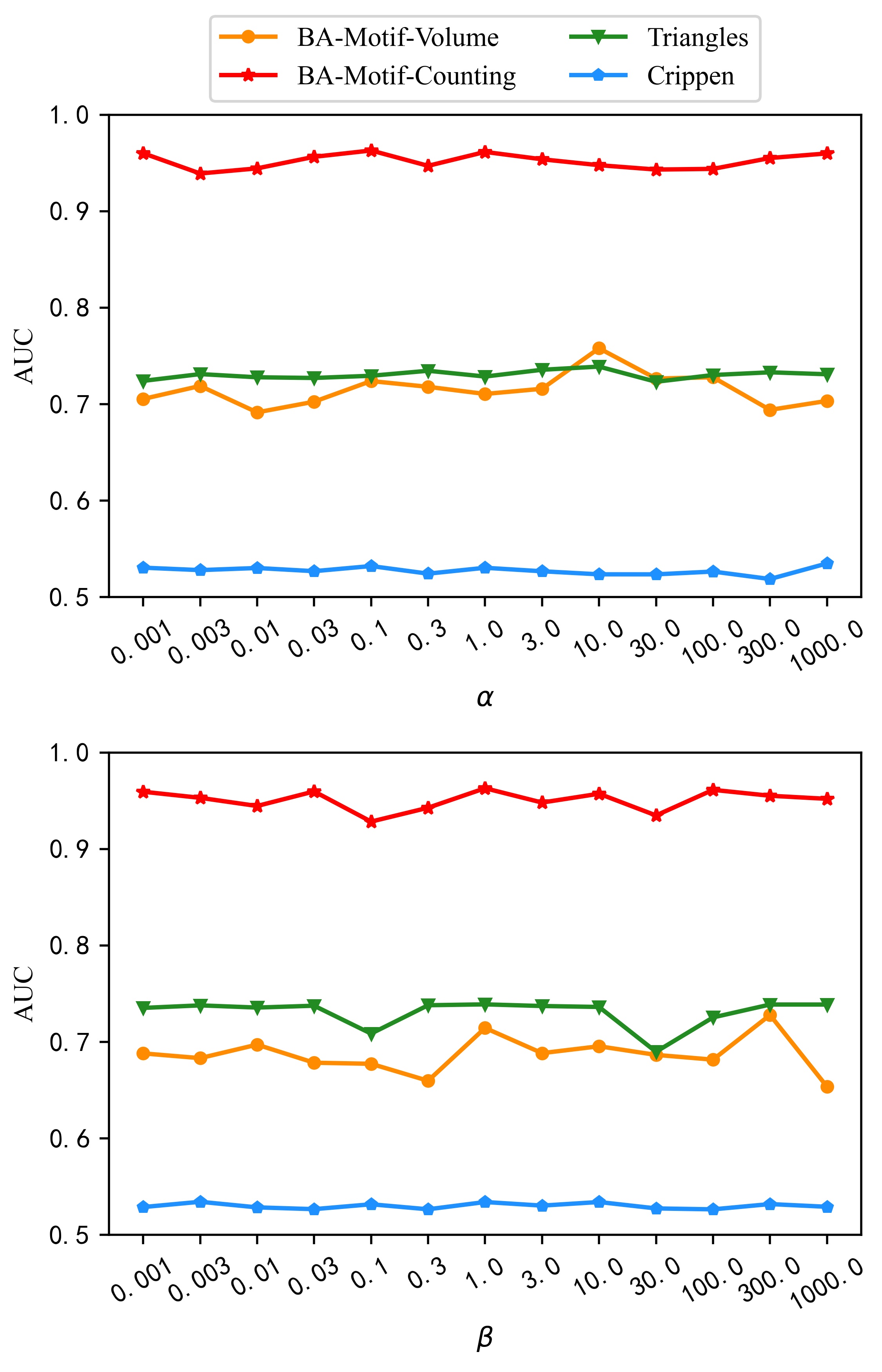
Figure 6. Hyper-parameters study of $\alpha$ and $\beta$ on four datasets with RegExplainer. In both figures, the x-axis is the value of different hyper-parameter settings and the y-axis is the value of the average AUC score over ten runs with different random seeds.

4.5. Study the Decision Boundary and the Distributions Numerically

In this section, we visualize the regression values of the graphs and calculate the prediction shifting distance for each dataset and analyze their correlations to the distance of the decision boundaries. We put our results into Figure 7 and Table 2.

We observed that in Figure 7, the red points distribute surround the blue points but the green points are shifted away, which indicates that the explanation sub-graph couldn’t help GNNs make correct predictions. As shown in Table 2, we calculate the RMSE score between [the] $f(G)$ and $Y$, $f(G^{*})$ and $Y$, $f(G)$ and $f(G^{*})$ respectively, where $f(G)$ is the prediction the original graph, $f(G^{*}$ is the prediction of the explanation sub-graph, and $Y$ is the regression label. We could observe that $f(G^{*})$ shows a significant prediction shifting from $f(G)$ and $Y$, indicating that the mutual information calculated with the original GIB objective Eq.( 2) would be biased.

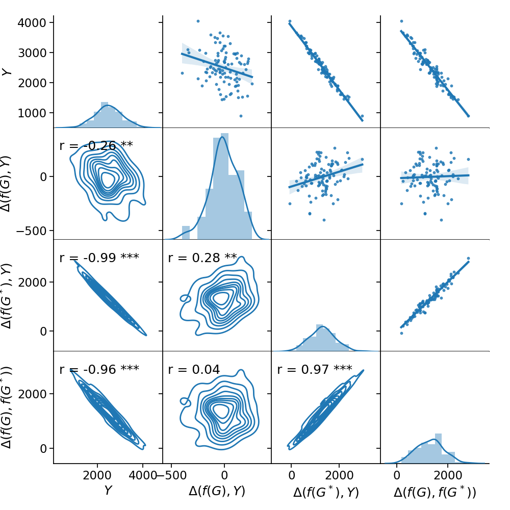
Figure 7. Correlations between the predictions and their shifting on BA-Motif-Volume. The value of $r$ indicates the Pearson Correlation Coefficient, and the values with * indicate statistical significance for correlation, where *** indicates the p-value for testing non-correlation $p\leq 0.001$. Each point represents one graph instance.

We further explore the relationship of the prediction shifting against the label value with dataset BA-Motif-Volume, which represents the semantic decision boundary. In Figure 7, each point represents a graph instance, where $Y$ represents the ground-truth label, and $\Delta$ represents the absolute value difference. It’s clear that both the $\Delta(f(G^{*}),Y)$ and $\Delta(f(G),f(G^{*}))$ strongly correlated to $Y$ with statistical significance, indicating the prediction shifting problem is related to the continuous ordered decision boundary, which is present in regression tasks.

5. Related Works

GNN explainability: The explanation methods for GNN models could be categorized into two types based on their granularity: instance-level (Shan et al., 2021b; Ying et al., 2019; Luo et al., 2020; Yuan et al., 2021) and model-level (Yuan et al., 2020), where the former methods explain the prediction for each instance by identifying important sub-graphs, and the latter method aims to understand the global decision rules captured by the GNN. These methods could also be classified into two categories based on their methodology: self-explainable GNNs (Baldassarre and Azizpour, 2019; Dai and Wang, 2021) and post-hoc explanation methods (Ying et al., 2019; Luo et al., 2020; Yuan et al., 2021), where the former methods provide both predictions and explanations, while the latter methods use an additional model or strategy to explain the target GNN. Additionally, CGE (Fang et al., 2023b) (cooperative explanation) generates the sub-graph explanation with the sub-network simultaneously, by using cooperative learning. However, it has to treat the GNN model as a white-box, which is usually unavailable in the post-hoc explaining.

Existing methods haven’t explored the explanation of the graph regression task and haven’t considered two important challenges: the distribution shifting problem and the limitation of the GIB objective, which were addressed by our work.

Mix-up approach: We faced the challenge of the distribution shifting problem and adopted the mix-up (Zhang et al., 2017) approach in our work. The mix-up approach is a data augmentation technique that increases the diversity of the training data and improves the generalization performance of the model. There are also many mix-up related technologies including GraphMix (Verma et al., 2019), MixupGraph (Wang et al., 2021), G-Mixup (Han et al., 2022), and ifMixup (Guo and Mao, 2021). However, existing methods couldn’t address the distribution shifting problem in graph regression tasks and improve the explainability of GNN due to their inability to generate graphs into original distributions, which highlights the need for a new mix-up method. Thus, we develop a new mix-up approach in our work.

6. Conclusion

We addressed the challenges in the explainability of graph regression tasks and proposed the RegExplainer, a novel method for explaining the predictions of GNNs with the post-hoc explanation sub-graph on graph regression task without requiring modification of the underlying GNN architecture or re-training. We showed how RegExplainer can leverage the distribution shifting problem and knowledge from the continuous decision boundary with the mix-up approach and the adopted GIB objective with the contrastive loss, while the problems seriously affect the performances of other explainers. We formulated four new datasets, which are BA-Motif-Volume, BA-Motif-Counting, Triangles, and Crippen for evaluating the explainers on the graph regression task, which are developed from the previous datasets and follow a similar setting. They could also benefit future studies on the XAIG-R.

References

- (1)
- Baldassarre and Azizpour (2019) Federico Baldassarre and Hossein Azizpour. 2019. Explainability Techniques for Graph Convolutional Networks.
- Balın et al. (2019) Muhammed Fatih Balın, Abubakar Abid, and James Zou. 2019. Concrete autoencoders: Differentiable feature selection and reconstruction. In International conference on machine learning. PMLR, 444–453.
- Bongini et al. (2021) Pietro Bongini, Monica Bianchini, and Franco Scarselli. 2021. Molecular generative graph neural networks for drug discovery. Neurocomputing 450 (2021), 242–252.
- Brockschmidt (2020) Marc Brockschmidt. 2020. GNN-FiLM: Graph Neural Networks with Feature-wise Linear Modulation. arXiv:1906.12192 [cs.LG]
- Cai et al. (2021) Lei Cai, Jundong Li, Jie Wang, and Shuiwang Ji. 2021. Line graph neural networks for link prediction. IEEE Transactions on Pattern Analysis and Machine Intelligence 44, 9 (2021), 5103–5113.
- Chen et al. (2020) Zhengdao Chen, Lei Chen, Soledad Villar, and Joan Bruna. 2020. Can Graph Neural Networks Count Substructures? arXiv:2002.04025 [cs.LG]
- Chereda et al. (2019) Hryhorii Chereda, Annalen Bleckmann, Frank Kramer, Andreas Leha, and Tim Beissbarth. 2019. Utilizing Molecular Network Information via Graph Convolutional Neural Networks to Predict Metastatic Event in Breast Cancer.. In GMDS. 181–186.
- Dai and Wang (2021) Enyan Dai and Suhang Wang. 2021. Towards Self-Explainable Graph Neural Network.
- Delaney (2004) John S Delaney. 2004. ESOL: estimating aqueous solubility directly from molecular structure. Journal of chemical information and computer sciences 44, 3 (2004), 1000–1005.
- Fan et al. (2019) Wenqi Fan, Yao Ma, Qing Li, Yuan He, Eric Zhao, Jiliang Tang, and Dawei Yin. 2019. Graph Neural Networks for Social Recommendation.
- Fang et al. (2023a) Junfeng Fang, Xiang Wang, An Zhang, Zemin Liu, Xiangnan He, and Tat-Seng Chua. 2023a. Cooperative Explanations of Graph Neural Networks. In Proceedings of the Sixteenth ACM International Conference on Web Search and Data Mining. 616–624.
- Fang et al. (2023b) Junfeng Fang, Xiang Wang, An Zhang, Zemin Liu, Xiangnan He, and Tat-Seng Chua. 2023b. Cooperative Explanations of Graph Neural Networks. Association for Computing Machinery, New York, NY, USA, 616–624. https://doi.org/10.1145/3539597.3570378
- Fang et al. (2020) Tongtong Fang, Nan Lu, Gang Niu, and Masashi Sugiyama. 2020. Rethinking importance weighting for deep learning under distribution shift. Advances in neural information processing systems 33 (2020), 11996–12007.
- Guo and Mao (2021) Hongyu Guo and Yongyi Mao. 2021. ifmixup: Towards intrusion-free graph mixup for graph classification. arXiv e-prints (2021), arXiv–2110.
- Han et al. (2022) Xiaotian Han, Zhimeng Jiang, Ninghao Liu, and Xia Hu. 2022. G-mixup: Graph data augmentation for graph classification. In International Conference on Machine Learning. PMLR, 8230–8248.
- Henaff et al. (2015) Mikael Henaff, Joan Bruna, and Yann LeCun. 2015. Deep Convolutional Networks on Graph-Structured Data. arXiv:1506.05163 [cs.LG]
- Hendrycks and Gimpel (2016) Dan Hendrycks and Kevin Gimpel. 2016. A baseline for detecting misclassified and out-of-distribution examples in neural networks. arXiv preprint arXiv:1610.02136 (2016).
- Jia and Benson (2020) Junteng Jia and Austion R Benson. 2020. Residual correlation in graph neural network regression. In Proceedings of the 26th ACM SIGKDD International Conference on Knowledge Discovery & Data Mining. 588–598.
- Lee et al. (2018) John Boaz Lee, Ryan Rossi, and Xiangnan Kong. 2018. Graph classification using structural attention. In Proceedings of the 24th ACM SIGKDD International Conference on Knowledge Discovery & Data Mining. 1666–1674.
- Li et al. (2017) Jundong Li, Kewei Cheng, Suhang Wang, Fred Morstatter, Robert P. Trevino, Jiliang Tang, and Huan Liu. 2017. Feature Selection: A Data Perspective. ACM Comput. Surv. 50, 6, Article 94 (dec 2017), 45 pages. https://doi.org/10.1145/3136625
- Li and Zhu (2021) Mengzhang Li and Zhanxing Zhu. 2021. Spatial-Temporal Fusion Graph Neural Networks for Traffic Flow Forecasting. Proceedings of the AAAI Conference on Artificial Intelligence 35, 5 (May 2021), 4189–4196.
- Li et al. (2022) Yiqiao Li, Jianlong Zhou, Sunny Verma, and Fang Chen. 2022. A survey of explainable graph neural networks: Taxonomy and evaluation metrics. arXiv preprint arXiv:2207.12599 (2022).
- Liu et al. (2021) Xu Liu, Yingguang Li, Qinglu Meng, and Gengxiang Chen. 2021. Deep transfer learning for conditional shift in regression. Knowledge-Based Systems 227 (2021), 107216.
- Longa et al. (2022) Antonio Longa, Steve Azzolin, Gabriele Santin, Giulia Cencetti, Pietro Liò, Bruno Lepri, and Andrea Passerini. 2022. Explaining the Explainers in Graph Neural Networks: a Comparative Study. arXiv preprint arXiv:2210.15304 (2022).
- Luo et al. (2020) Dongsheng Luo, Wei Cheng, Dongkuan Xu, Wenchao Yu, Bo Zong, Haifeng Chen, and Xiang Zhang. 2020. Parameterized explainer for graph neural network. Advances in neural information processing systems 33 (2020), 19620–19631.
- Mansimov et al. (2019) E. Mansimov, O. Mahmood, and S. Kang. 2019. Molecular Geometry Prediction using a Deep Generative Graph Neural Network. https://doi.org/10.1038/s41598-019-56773-5
- Miao et al. (2022) Siqi Miao, Mia Liu, and Pan Li. 2022. Interpretable and generalizable graph learning via stochastic attention mechanism. In International Conference on Machine Learning. PMLR, 15524–15543.
- Min et al. (2021) Shengjie Min, Zhan Gao, Jing Peng, Liang Wang, Ke Qin, and Bo Fang. 2021. STGSN — A Spatial–Temporal Graph Neural Network framework for time-evolving social networks. Knowledge-Based Systems 214 (2021), 106746.
- Rusek et al. (2022) Krzysztof Rusek, Paul Almasan, José Suárez-Varela, Piotr Chołda, Pere Barlet-Ros, and Albert Cabellos-Aparicio. 2022. Fast Traffic Engineering by Gradient Descent with Learned Differentiable Routing. arXiv:2209.10380 [cs.NI]
- Sanchez-Lengeling et al. (2020) Benjamin Sanchez-Lengeling, Jennifer Wei, Brian Lee, Emily Reif, Peter Wang, Wesley Qian, Kevin McCloskey, Lucy Colwell, and Alexander Wiltschko. 2020. Evaluating attribution for graph neural networks. Advances in neural information processing systems 33 (2020), 5898–5910.
- Scarselli et al. (2009) Franco Scarselli, Marco Gori, Ah Chung Tsoi, Markus Hagenbuchner, and Gabriele Monfardini. 2009. The Graph Neural Network Model. IEEE Transactions on Neural Networks 20, 1 (2009), 61–80.
- Shaikh et al. (2017) Shakila Shaikh, Sheetal Rathi, and Prachi Janrao. 2017. Recommendation system in e-commerce websites: a graph based approached. In 2017 IEEE 7th International Advance Computing Conference (IACC). IEEE, 931–934.
- Shan et al. (2021a) Caihua Shan, Yifei Shen, Yao Zhang, Xiang Li, and Dongsheng Li. 2021a. Reinforcement Learning Enhanced Explainer for Graph Neural Networks. In Advances in Neural Information Processing Systems, A. Beygelzimer, Y. Dauphin, P. Liang, and J. Wortman Vaughan (Eds.). https://openreview.net/forum?id=nUtLCcV24hL
- Shan et al. (2021b) Caihua Shan, Yifei Shen, Yao Zhang, Xiang Li, and Dongsheng Li. 2021b. Reinforcement Learning Enhanced Explainer for Graph Neural Networks. In Advances in Neural Information Processing Systems, M. Ranzato, A. Beygelzimer, Y. Dauphin, P.S. Liang, and J. Wortman Vaughan (Eds.), Vol. 34. Curran Associates, Inc., 22523–22533. https://proceedings.neurips.cc/paper/2021/file/be26abe76fb5c8a4921cf9d3e865b454-Paper.pdf
- Sorokin and Gurevych (2018) Daniil Sorokin and Iryna Gurevych. 2018. Modeling Semantics with Gated Graph Neural Networks for Knowledge Base Question Answering. In Proceedings of the 27th International Conference on Computational Linguistics. Association for Computational Linguistics, Santa Fe, New Mexico, USA, 3306–3317. https://aclanthology.org/C18-1280
- Tishby et al. (2000) Naftali Tishby, Fernando C Pereira, and William Bialek. 2000. The information bottleneck method. arXiv preprint physics/0004057 (2000).
- Tishby and Zaslavsky (2015) Naftali Tishby and Noga Zaslavsky. 2015. Deep learning and the information bottleneck principle. In 2015 ieee information theory workshop (itw). IEEE, 1–5.
- van den Oord et al. (2019) Aaron van den Oord, Yazhe Li, and Oriol Vinyals. 2019. Representation Learning with Contrastive Predictive Coding. arXiv:1807.03748 [cs.LG]
- Veličković et al. (2017) Petar Veličković, Guillem Cucurull, Arantxa Casanova, Adriana Romero, Pietro Lio, and Yoshua Bengio. 2017. Graph attention networks. arXiv preprint arXiv:1710.10903 (2017).
- Verma et al. (2019) Vikas Verma, Meng Qu, Alex Lamb, Yoshua Bengio, Juho Kannala, and Jian Tang. 2019. GraphMix: Regularized Training of Graph Neural Networks for Semi-Supervised Learning. CoRR abs/1909.11715 (2019).
- Wang et al. (2020) Xiaoyang Wang, Yao Ma, Yiqi Wang, Wei Jin, Xin Wang, Jiliang Tang, Caiyan Jia, and Jian Yu. 2020. Traffic Flow Prediction via Spatial Temporal Graph Neural Network. In Proceedings of The Web Conference 2020 (Taipei, Taiwan) (WWW ’20). Association for Computing Machinery, New York, NY, USA, 1082–1092.
- Wang et al. (2021) Yiwei Wang, Wei Wang, Yuxuan Liang, Yujun Cai, and Bryan Hooi. 2021. Mixup for node and graph classification. In Proceedings of the Web Conference 2021. 3663–3674.
- Wildman and Crippen (1999) Scott A Wildman and Gordon M Crippen. 1999. Prediction of physicochemical parameters by atomic contributions. Journal of chemical information and computer sciences 39, 5 (1999), 868–873.
- Wiles et al. (2021) Olivia Wiles, Sven Gowal, Florian Stimberg, Sylvestre Alvise-Rebuffi, Ira Ktena, Krishnamurthy Dvijotham, and Taylan Cemgil. 2021. A fine-grained analysis on distribution shift. arXiv preprint arXiv:2110.11328 (2021).
- Wu et al. (2022a) Bingzhe Wu, Jintang Li, Junchi Yu, Yatao Bian, Hengtong Zhang, CHaochao Chen, Chengbin Hou, Guoji Fu, Liang Chen, Tingyang Xu, et al. 2022a. A survey of trustworthy graph learning: Reliability, explainability, and privacy protection. arXiv preprint arXiv:2205.10014 (2022).
- Wu et al. (2022b) Shiwen Wu, Fei Sun, Wentao Zhang, Xu Xie, and Bin Cui. 2022b. Graph Neural Networks in Recommender Systems: A Survey. ACM Comput. Surv. 55, 5, Article 97 (dec 2022), 37 pages. https://doi.org/10.1145/3535101
- Wu et al. (2020) Tailin Wu, Hongyu Ren, Pan Li, and Jure Leskovec. 2020. Graph information bottleneck. Advances in Neural Information Processing Systems 33 (2020), 20437–20448.
- Wu et al. (2019) Zonghan Wu, Shirui Pan, Guodong Long, Jing Jiang, and Chengqi Zhang. 2019. Graph Wavenet for Deep Spatial-Temporal Graph Modeling. In Proceedings of the 28th International Joint Conference on Artificial Intelligence (Macao, China) (IJCAI’19). AAAI Press, 1907–1913.
- Xiao et al. (2022) Shunxin Xiao, Shiping Wang, Yuanfei Dai, and Wenzhong Guo. 2022. Graph neural networks in node classification: survey and evaluation. Machine Vision and Applications 33 (2022), 1–19.
- Xie et al. (2022) Yaochen Xie, Sumeet Katariya, Xianfeng Tang, Edward Huang, Nikhil Rao, Karthik Subbian, and Shuiwang Ji. 2022. Task-Agnostic Graph Explanations. arXiv:2202.08335 [cs.LG]
- Xiong et al. (2019) Zhaoping Xiong, Dingyan Wang, Xiaohong Liu, Feisheng Zhong, Xiaozhe Wan, Xutong Li, Zhaojun Li, Xiaomin Luo, Kaixian Chen, Hualiang Jiang, et al. 2019. Pushing the boundaries of molecular representation for drug discovery with the graph attention mechanism. Journal of medicinal chemistry 63, 16 (2019), 8749–8760.
- Yang and Toni (2018) Kaige Yang and Laura Toni. 2018. Graph-based recommendation system. In 2018 IEEE Global Conference on Signal and Information Processing (GlobalSIP). IEEE, 798–802.
- Ying et al. (2019) Zhitao Ying, Dylan Bourgeois, Jiaxuan You, Marinka Zitnik, and Jure Leskovec. 2019. Gnnexplainer: Generating explanations for graph neural networks. Advances in neural information processing systems 32 (2019). https://doi.org/10.48550/ARXIV.1903.03894
- Yu et al. (2018) Bing Yu, Haoteng Yin, and Zhanxing Zhu. 2018. Spatio-Temporal Graph Convolutional Networks: A Deep Learning Framework for Traffic Forecasting. In Proceedings of the Twenty-Seventh International Joint Conference on Artificial Intelligence, IJCAI-18. International Joint Conferences on Artificial Intelligence Organization, 3634–3640.
- Yu et al. (2020) Junchi Yu, Tingyang Xu, Yu Rong, Yatao Bian, Junzhou Huang, and Ran He. 2020. Graph information bottleneck for subgraph recognition. arXiv preprint arXiv:2010.05563 (2020).
- Yuan et al. (2020) Hao Yuan, Jiliang Tang, Xia Hu, and Shuiwang Ji. 2020. XGNN: Towards Model-Level Explanations of Graph Neural Networks. In KDD ’20: The 26th ACM SIGKDD Conference on Knowledge Discovery and Data Mining, Virtual Event, CA, USA, August 23-27, 2020. ACM, 430–438.
- Yuan et al. (2022) Hao Yuan, Haiyang Yu, Shurui Gui, and Shuiwang Ji. 2022. Explainability in graph neural networks: A taxonomic survey. IEEE Transactions on Pattern Analysis and Machine Intelligence (2022).
- Yuan et al. (2021) Hao Yuan, Haiyang Yu, Jie Wang, Kang Li, and Shuiwang Ji. 2021. On explainability of graph neural networks via subgraph explorations. In International Conference on Machine Learning. PMLR, 12241–12252.
- Zhang et al. (2017) Hongyi Zhang, Moustapha Cisse, Yann N. Dauphin, and David Lopez-Paz. 2017. Mixup: Beyond Empirical Risk Minimization. https://doi.org/10.48550/ARXIV.1710.09412
- Zhang et al. (2022) He Zhang, Bang Wu, Xingliang Yuan, Shirui Pan, Hanghang Tong, and Jian Pei. 2022. Trustworthy graph neural networks: Aspects, methods and trends. arXiv preprint arXiv:2205.07424 (2022).
- Zhang et al. (2023) Jiaxing Zhang, Dongsheng Luo, and Hua Wei. 2023. MixupExplainer: Generalizing Explanations for Graph Neural Networks with Data Augmentation. In Proceedings of 29th ACM SIGKDD Conference on Knowledge Discovery and Data Mining (SIGKDD).
- Zhang and Chen (2018) Muhan Zhang and Yixin Chen. 2018. Link prediction based on graph neural networks. Advances in neural information processing systems 31 (2018).
- Zhang et al. (2018) Muhan Zhang, Zhicheng Cui, Marion Neumann, and Yixin Chen. 2018. An end-to-end deep learning architecture for graph classification. In Proceedings of the AAAI conference on artificial intelligence, Vol. 32.
- Zhang and Sabuncu (2018) Zhilu Zhang and Mert Sabuncu. 2018. Generalized cross entropy loss for training deep neural networks with noisy labels. Advances in neural information processing systems 31 (2018).
- Zhao et al. (2019) Long Zhao, Xi Peng, Yu Tian, Mubbasir Kapadia, and Dimitris N Metaxas. 2019. Semantic graph convolutional networks for 3d human pose regression. In Proceedings of the IEEE/CVF conference on computer vision and pattern recognition. 3425–3435.