MixupExplainer: Generalizing Explanations for Graph Neural Networks with Data Augmentation

Abstract.

Graph Neural Networks (GNNs) have received increasing attention due to their ability to learn from graph-structured data. However, their predictions are often not interpretable. Post-hoc instance-level explanation methods have been proposed to understand GNN predictions. These methods seek to discover substructures that explain the prediction behavior of a trained GNN. In this paper, we shed light on the existence of the distribution shifting issue in existing methods, which affects explanation quality, particularly in applications on real-life datasets with tight decision boundaries. To address this issue, we introduce a generalized Graph Information Bottleneck (GIB) form that includes a label-independent graph variable, which is equivalent to the vanilla GIB. Driven by the generalized GIB, we propose a graph mixup method, MixupExplainer, with a theoretical guarantee to resolve the distribution shifting issue. We conduct extensive experiments on both synthetic and real-world datasets to validate the effectiveness of our proposed mixup approach over existing approaches. We also provide a detailed analysis of how our proposed approach alleviates the distribution shifting issue.

1. Introduction

Graph Neural Networks (GNNs) (Scarselli et al., 2009), a powerful technology for learning knowledge from graph-structured data, are gaining increasing attention in today’s world, where graph-structured data such as social networks (Feng et al., 2023; Min et al., 2021), molecular structures (Chereda et al., 2019; Mansimov et al., 2019), traffic flows (Wang et al., 2020; Li and Zhu, 2021; Wu et al., 2019; Lei et al., 2022), and knowledge graphs (Sorokin and Gurevych, 2018) are widely used. GNNs work by propagating and fusing messages from neighboring nodes on the graph using message-passing mechanisms. These networks have achieved state-of-the-art performance in tasks like node classification, graph classification, graph regression, and link prediction.

Despite their success, GNNs, like other neural networks, lack interpretability. Understanding how GNNs make predictions is crucial for several reasons. First, it can increase user confidence when using GNNs in high-stakes applications (Yuan et al., 2022; Longa et al., 2022). Second, it enhances the transparency of the models, making them suitable for use in sensitive fields such as healthcare and drug discovery, where fairness, privacy, and safety are critical concerns (Zhang et al., 2022; Wu et al., 2022; Li et al., 2022). Thus, exploring the interpretability of GNNs is essential.

A common solution to improve GNN models’ transparency is applying post-hoc instance-level explainability methods. These methods identify key substructures in input graphs to explain predictions made by trained GNN models, making it easier for humans to understand the models’ inner workings. Examples of such methods include GNNExplainer (Ying et al., 2019), which determines the importance of nodes and edges through perturbation, and PGExplainer(Luo et al., 2020), which trains a graph generator to incorporate global information. Recent studies in the field (Fang et al., 2023; Shan et al., 2021a) also contribute to the development of these methods. Post-hoc explainability methods can be classified under a label-preserving framework, where the explanation is a substructure of the original graph and preserves the information about the predicted label. On top of the intuitive principle, Graph Information Bottleneck (GIB) (Wu et al., 2020; Miao et al., 2022; Yu et al., 2020) maximizes the mutual information $I(G^{*},Y)$ between the target label $Y$ and the explanation $G^{*}$ while constraining the size of the explanation as the mutual information between the original graph $G$ and the explanation $G^{*}$.

Approximating the mutual information between the label $Y$ and explanation $G^{*}$ is challenging due to its intractability, so previous works (Ying et al., 2019; Luo et al., 2020; Miao et al., 2022) usually estimate $I(G^{*},Y)$ using $I(f(G^{*}),Y)$, the mutual information between the predictions $f(G^{*})$ from GNN model $f$ and its label $Y$. However, this approximation overlooks the distribution shifting issue between the original graph $G$ and explanation $G^{*}$ after the processing of the prediction model $f$. Due to differences in properties like the number of nodes or the structures in $G$, $G^{*}$ could have a different distribution from $G$. As seen in Figure 1, the visualization of the embeddings for the original graph and its explanation shows that the explanation embeddings are out of distribution with respect to the original graphs, which leads to impaired safe usage of the approximation because of the inductive bias in $f$. The negative impact of the distribution shifting problem on explanation quality is especially pronounced when applied to complex real-world datasets with tight decision boundaries.

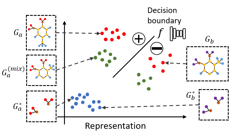
Figure 1. Visualization of original graphs $G$, explanation subgraphs $G^{*}$, and our generated graphs $G^{(\text{mix})}$. There is a large distributional divergence between explanation subgraphs $G^{*}$ and original graphs $G$. $G_{a}$ and $G_{b}$ are two graphs in the original dataset. More experimental results on the existence of the distributional divergence can be found in Section 5.3.

While the distribution shifting issue in post-hoc explanations has gained growing attention in computer vision (Chang et al., 2018), this issue is less explored in the graph domain. In computer vision,  (Chang et al., 2018) optimizes image classifier explanations to highlight contextual information relevant to the prediction and consistent with the training distribution.  (Qiu et al., 2022) addresses the distribution shifting issue in image explanation via a module that quantifies affinity between perturbed data and original dataset distribution. In the graph domain, while a recent work (Fang et al., 2023) attempts to address distribution shifting by annealing the size constraint coefficient at the start of the explanation process, the distribution shifting issue still persists throughout the explanation process.

To address the distribution shifting issue in post-hoc graph explanation, we introduce a general form of Graph Information Bottleneck (GIB) that includes another label-independent graph variable $G^{\Delta}$. This new form of GIB is proven equivalent to vanilla GIB. By having $G^{\Delta}$ in the objective, we can alleviate the distribution shifting problem with theoretical guarantees. To further improve the explanation method, we propose MixupExplainer using an improved Mixup approach. The MixupExplainer assumes that a non-explainable part of a graph is label-independent and mixes the explanation with a non-explainable structure from another randomly sampled graph. The explanation substructure is obtained by minimizing the difference between the predicted labels of the original graph and the mixup graph.

To the end, we summarize our contributions as follows.

• For the first time, we point out that the distribution shifting problem is prevalent in the most popular post-hoc explanation framework for graph neural networks.

• We derive a generalized framework with a solid theoretical foundation to alleviate the problem and propose a straightforward yet effective instantiation based on mixing up the explanation with a randomly sampled base structure by aligning the graph and mixing the graph masks.

• Comprehensive empirical studies on both synthetic and real-life datasets demonstrate that our method can dramatically and consistently improve the quality of the explanations, with up to $35.5\%$ in AUC scores.

2. Related Work

2.1. Graph Neural Networks

The use of graph neural networks (GNNs) is on the rise for analyzing graph structure data, as seen in recent research studies (Dai et al., 2022; Feng et al., 2023; Hamilton et al., 2017). There are two main types of GNNs: spectral-based approaches (Bruna et al., 2013; Kipf and Welling, 2016; Tang et al., 2019) and spatial-based approaches (Atwood and Towsley, 2016; Duvenaud et al., 2015; Xiao et al., 2021). Despite the differences, message passing is a common framework for both, using pattern extraction and message interaction between layers to update node embeddings. However, GNNs are still considered a black box model with a hard-to-understand mechanism, particularly for graph data, which is harder to interpret compared to image data. To fully utilize GNNs, especially in high-risk applications, it is crucial to develop methods for understanding how they work.

2.2. GNN Explanation

Many attempts have been made to interpret GNN models and explain their predictions (Shan et al., 2021b; Ying et al., 2019; Luo et al., 2020; Yuan et al., 2021; Spinelli et al., 2022; Wang et al., 2021b). These methods can be grouped into two categories based on granularity: (1) instance-level explanation, which explains the prediction for each instance by identifying significant substructures (Ying et al., 2019; Yuan et al., 2021; Shan et al., 2021b), and (2) model-level explanation, which seeks to understand the global decision rules captured by the GNN (Luo et al., 2020; Spinelli et al., 2022; Baldassarre and Azizpour, 2019). From a methodological perspective, existing methods can be classified as (1) self-explainable GNNs (Baldassarre and Azizpour, 2019; Dai and Wang, 2021), where the GNN can provide both predictions and explanations, and (2) post-hoc explanations (Ying et al., 2019; Luo et al., 2020; Yuan et al., 2021), which use another model or strategy to explain the target GNN. In this work, we focus on post-hoc instance-level explanations, which involve identifying instance-wise critical substructures to explain the prediction. Various strategies have been explored, including gradient signals, perturbed predictions, and decomposition.

Perturbed prediction-based methods are the most widely used in post-hoc instance-level explanations. The idea is to learn a perturbation mask that filters out non-important connections and identifies dominant substructures while preserving the original predictions. For example, GNNExplainer (Ying et al., 2019) uses end-to-end learned soft masks on node attributes and graph structure, while PGExplainer (Luo et al., 2020) incorporates a graph generator to incorporate global information. RG-Explainer (Shan et al., 2021b) uses reinforcement learning technology with starting point selection to find important substructures for the explanation.

However, most of these methods fail to consider the distribution shifting issue. The explanation should contain the same information that contributes to the prediction, but the GNN is trained on a data pattern that consists of an explanation subgraph relevant to labels, and a label-independent structure, leading to a distribution shifting problem when feeding the explanation directly into the GNN. Our method aims to capture the distribution information of the graph and build the explanation with a label-independent structure to help the explainer better minimize the objective function and retrieve a higher-quality explanation.

2.3. Graph Data Augmentation with Mixup

Data augmentation addresses issues such as noise, scarcity, and out-of-distribution problems. One popular data augmentation approach is using Mixup (Zhang et al., 2017) strategy to generate synthetic training examples based on feature mixing and label mixing. Specifically, (Verma et al., 2021; Wang et al., 2021a) mix the graph representation learned from GNNs to avoid dealing with the arbitrary structure in the input space for mixing a node or graph pair. ifMixup (Guo and Mao, 2021) interpolates both the node features and the edges of the input pair based on feature mixing and graph generation.  (Han et al., 2022) and  (Wu et al., 2021) generate interpolated graphs with the estimation of the properties in the graph data, like the graphon of each class or nearest neighbors of target nodes. All the previous methods (Verma et al., 2019, 2021; Han et al., 2022; Wang et al., 2021a; Guo and Mao, 2021) aim to generalize the mixup approach to improve the performance of classification models like GNNs. Unlike existing graph mixup approaches, this paper solves a different task, which is to generalize the explanations for GNN.

3. Preliminary

3.1. Notations and Problem Definition

We denote a graph as $G=(\mathcal{V},\mathcal{E};{\bm{X}},{\bm{A}})$, where $\mathcal{V}=\{v_{1},v_{2},...,v_{n}\}$ represents a set of $n$ nodes and $\mathcal{E}\in\mathcal{V}\times\mathcal{V}$ represents the edge set. Each graph has a feature matrix ${\bm{X}}\in{\mathbb{R}}^{n\times d}$ for the nodes, where in ${\bm{X}}$, ${\bm{x}}_{i}\in{\mathbb{R}}^{1\times d}$ is the $d$-dimensional node feature of node $v_{i}$. $\mathcal{E}$ is described by an adjacency matrix ${\bm{A}}\in\{0,1\}^{n\times n}$. ${A}_{ij}=1$ means that there is an edge between node $v_{i}$ and $v_{j}$; otherwise, ${A}_{ij}=0$.

For graph classification task, each graph $G_{i}$ has a label $Y_{i}\in\mathcal{C}$, with a GNN model $f$ trained to classify $G_{i}$ into its class, i.e., $f:({\bm{X}},{\bm{A}})\mapsto\{1,2,...,C\}$. For the node classification task, each graph $G_{i}$ denotes a $K$-hop sub-graph centered around node $v_{i}$, with a GNN model $f$ trained to predict the label for node $v_{i}$ based on the node representation of $v_{i}$ learned from $G_{i}$.

Problem 1 (Post-hoc Instance-level GNN Explanation).

Given a trained GNN model $f$, for an arbitrary input graph $G=(\mathcal{V},\mathcal{E};{\bm{X}},{\bm{A}})$, the goal of post-hoc instance-level GNN explanation is to find a subgraph $G^{*}$ that can explain the prediction of $f$ on $G$.

Informative feature selection has been well studied in non-graph structured data (Li et al., 2017), and traditional methods, such as concrete autoencoder (Balın et al., 2019), can be directly extended to explain features in GNNs. In this paper, we focus on discovering important typologies. Formally, the obtained explanation $G^{*}$ is depicted by a binary mask ${\bm{M}}\in\{0,1\}^{n\times n}$ on the adjacency matrix, e.g., $G^{*}=({\mathcal{V}},{\mathcal{E}},{\bm{A}}\odot{\bm{M}};{\bm{X}})$, $\odot$ means elements-wise multiplication. The mask highlights components of $G$ which are essential for $f$ to make the prediction.

3.2. Graph Information Bottleneck

The Information Bottleneck (IB) (Tishby et al., 2000; Tishby and Zaslavsky, 2015) provides an intuitive principle for learning dense representations that an optimal representation should contain minimal and sufficient information for the downstream prediction task. Based on IB, a recent work unifies the most existing post-hoc explanation methods for GNN, such as GNNExplainer (Ying et al., 2019), PGExplainer (Luo et al., 2020), with the graph information bottleneck (GIB) principle (Wu et al., 2020; Miao et al., 2022; Yu et al., 2020). Formally, the objective of explaining the prediction of $f$ on $G$ can be represented by

(1) $$\operatorname*{arg\,min}_{G^{*}}I(G,G^{*})-\alpha I(G^{*},Y),$$

where $G^{*}$ is the explanation subgraph, $Y$ is the original or ground truth label, and $\alpha$ is a hyper-parameter to get the trade-off between minimal and sufficient constraints. GIB uses the mutual information $I(G,G^{*})$ to select the minimal explanation that inherits only the most indicative information from $G$ to predict the label $Y$ by maximizing $I(G^{*},Y)$, where $I(G,G^{*})$ avoids imposing potentially biased constraints, such as the size or the connectivity of the selected subgraphs (Miao et al., 2022). Through the optimization of the subgraph, $G^{*}$ provides model interpretation. Further, from the definition of mutual information, we have $I(G^{*},Y)=H(Y)-H(Y|G^{*})$, where the entropy $H(Y)$ is static and independent of the explanation process. Thus, minimizing the mutual information between the explanation subgraph $G^{*}$ and $Y$ can be reformulated as maximizing the conditional entropy of $Y$ given $G^{*}$. Formally, we rewrite the GIB objective as follows:

(2) $$\operatorname*{arg\,min}_{G^{*}}{I(G,G^{*})+\alpha H(Y|G^{*})},$$

As is shown in Figure 2(a), the objective function in Eq. (2) optimizes $G^{*}$ to have the minimal mutual information with the original graph $G$, which could be expressed as a subgraph from $G$ with a smaller size, or scattered components in $G$, while at the same time provides maximum mutual information for $Y$, which is equivalent to have minimum entropy $H(Y|G^{*})$.

Due to the intractability of entropy of the label conditioned on explanation, a widely-adopted approximation in previous methods (Ying et al., 2019; Luo et al., 2020; Zhao et al., 2023) is:

(3) $$\operatorname*{arg\,min}_{G^{*}}{I(G,G^{*})+\alpha H(Y|G^{*})}\approx\operatorname*{arg\,min}_{G^{*}}{I(G,G^{*})+\alpha CE(Y,Y^{*})},$$

where $Y^{*}=f(G^{*})$ is the predicted label of $G^{*}$ made by the model to be explained, $f$ and the cross-entropy $\text{CE}(Y,Y^{*})$ between the ground truth label $Y$ and $Y^{*}$ is used to approximate $H(Y|G^{*})$.

4. Methodology

In this section, we first introduce an overlooked problem in the GIB objective. Then we propose a generalized GIB objective to address the problem, which directly inspires our method through a mixup approach.

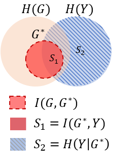
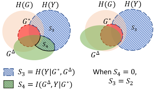
(a) Previous GIB Objective	(b) Our Generalized GIB Objective

Figure 2. Illustration of GIB and our proposed new objective. (a) Previous vanilla GIB objective aims to minimize $I(G^{*},Y)$ and $H(Y|G^{*})$, with a smaller overlap between $G^{*}$ and $G$. (b) Our generalized GIB objective has the same objective as vanilla GIB, with a larger lap between $G$ and $G^{*}+G^{\Delta}$, resulting in less distribution shifting issue.

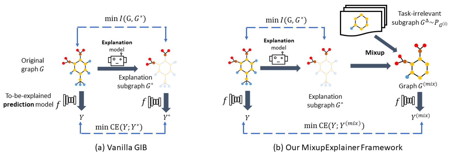
Figure 3. Illustration of the GIB-based explanation and our proposed MixupExplainer. (a) Vanilla GIB directly minimizes $\text{CE}(Y,Y^{*})$, which is the cross entropy between the original prediction $Y$ and the prediction of explanation subgraph $G^{*}$ made by the to-be-explained model $f$. (b) Our MixupExplainer first generates an augmented graph $G^{(\text{mix})}$ by mixing up the explanation subgraph $G^{*}$ with the label-independent part from another randomly sampled graph. Then we minimize the cross entropy between $Y$ and $Y^{\text{(mix)}}$, the prediction made by $f$ on $G^{(\text{mix})}$.

4.1. Generalized GIB

4.1.1. Diverging Distributions in Eq. (3)

Although prevalent, the approximation with $Y^{*}=f(G^{*})$ in Eq. (3) overlooks the distributional divergence between the original graph $G$ and the dense subgraph $G^{*}$ after the processing of the prediction model $f$. An intuitive example from the MUTAG dataset (Debnath et al., 1991) is shown in Figure 1. The prediction model $f$, represented by a hypothesis line, performs well in classifying the positive and negative samples. Due to the distribution shifting problem naturally inherent in $f(G)$ and $f(G^{*})$ on explanation subgraphs, $f$ maps some explanation subgraphs across the decision boundary to the negative region. As a result, the explanation subgraph achieved by Eq. (3) may be suboptimal and even far away from the ground truth explanation due to the significant divergence between $f(G^{*})$ and $f(G)$. The existing GIB framework could work for simple synthetic datasets by relying on the implicit knowledge associated with the class and assuming a large decision margin between the two or more classes. However, in more practical scenarios like MUTAG, the existing approximation may be heavily affected by the distribution shifting problem (Miao et al., 2022; Fang et al., 2023).

4.1.2. Addressing with Label-independent Subgraph

To address the above challenge in the previous GIB methods, we first generalize the existing GIB framework by taking a label-independent subgraph $G^{\Delta}$ into consideration. The intuition is that for an original graph $G_{a}$ with label $Y_{a}$, the label-independent subgraph $G_{a}^{\Delta}$ also contains useful information. For example, $G_{a}^{\Delta}$ makes sure that connecting it with the label-preserving subgraph $G_{a}^{*}$ will not lead to another label. Formally, given a graph variable $G^{\Delta}$ that satisfies $I(G^{\Delta},Y|G^{*})=0$, the GIB objective can be generalized as follows.

(4) $$\operatorname*{arg\,min}_{G^{*}}{I(G,G^{*})+\alpha H(Y|G^{*},G^{\Delta})},\quad\text{s.t. }\quad I(G^{\Delta},Y|G^{*})=0.$$

As shown below, our generalized GIB has the following property.

Property 1. The generalized GIB objective, Eq. (4) is equivalent to vanilla GIB, Eq. (2).

This can be proved by the definition of conditional entropy. With the condition that $I(G^{\Delta},Y|G^{*})=0$, we have $H(Y|G^{*})=H(Y|G^{*})+I(G^{\Delta},Y|G^{*})=H(Y|G^{*},G^{\Delta})$. Thus, the optimal solutions of GIB and our generalized version are equivalent. In addition, the advantage of our objective is that by choosing a suitable $G^{\Delta}$ that minimizes the distribution distance, $D(G^{*}+G^{\Delta},G)$, we can approximate the GIB without including the distribution shifting problem. An intuitive illustration is given in Figure 2(b).

Following exiting work (Ying et al., 2019; Luo et al., 2020), we can further approximate $H(Y|G^{*},G^{\Delta})$ with $\text{CE}(Y,Y^{m})$, where $Y^{m}=f(G^{*}+G^{\Delta})$ is the predicted label of $G^{*}+G^{\Delta}$ made by the model $f$ to be explained. Especially when $G^{\Delta}$ is an empty graph, our objective degenerates to the vanilla approximation. Formally, we derive our new objective for GNN explanation as follows:

(5) $$\operatorname*{arg\,min}_{G^{\Delta},G^{*}} {\quad I(G,G^{*})+\alpha\text{CE}(Y,Y^{m})}$$

$$\text{s.t. }\text{D}(G^{*}+G^{\Delta},G)=0,I(G^{\Delta},Y|G^{*})=0.$$

4.2. MixupExplainer

Inspired by Eq. 5, in this section, we introduce a straightforward yet theoretically guaranteed instantiation, MixupExplainer, to resolve the distribution shifting issue. Figure 3 demonstrates the overall framework of the proposed MixupExplainer and the differences between MixupExplainer and previous GIB methods. MixupExplainer includes a graph generation phase after extracting the explanation of the graph with the explainer. Specifically, we instantiate the $G^{\Delta}$ from the distribution of label-independent subgraphs from the graph dataset, denoted as ${\mathbb{P}}_{{\mathcal{G}}^{(i)}}$, and connect $G^{*}$ and $G^{\Delta}$ to generate a new graph $G^{(\text{mix})}$. Formally,

(6) $$G^{\Delta}\sim{\mathbb{P}}_{\mathcal{G}^{(i)}},\quad G^{(\text{mix})}=G^{*}+G^{\Delta}.$$

To avoid the trivial case that $G=G^{(\text{mix})}$, when sampling $G^{\Delta}$, we dismiss the original graph itself. In addition, since $G^{\Delta}$ is sampled without considering the label information, we can make a safe assumption that $I(G^{\Delta},Y|G^{*})=0$.

As stated in Problem 1, given a graph $G_{a}=({\bm{A}}_{a},{\bm{X}}_{a})$ and a to-be-explained model $f$, an explanation model $g$ aims to learns a subgraph $G^{*}_{a}$, represented with the edge mask ${\bm{M}}_{a}=g(G_{a})$ on the adjacency matrix ${\bm{A}}_{a}$. To generate a graph distributed similarly to $G_{a}$, we need to generate a label-independent subgraph, where we randomly sample another graph instance from the dataset, denoted by $G_{b}$, without considering the label information. With the explanation model $g$, we obtain the corresponding edge mask ${\bm{M}}_{b}$ for $G_{b}$. Then, we mix these two graphs by connecting the informative part in $G_{a}$ and the label-independent part in $G_{b}$. We first assume that $G_{a}$ and $G_{b}$ share the same set of nodes, and more general cases are discussed in the next section. Formally, the mask of the mixed graph, ${\bm{M}}_{a}^{(\text{mix})}$, is calculated as follows.

(7) $${\bm{M}}_{a}^{(\text{mix})}=\lambda{\bm{M}}_{a}+({\bm{A}}_{b}-\lambda{\bm{M}}_{b}),$$

where ${\bm{A}}_{b}$ is the adjacency matrix of graph $G_{b}$ and $\lambda$ is a hyper-parameter to support flexible usage of mixup operation. Then, we have $G^{(\text{mix})}_{a}=({\bm{X}}_{a},{\bm{M}}_{a}^{(\text{mix})})$. The mask matrix ${\bm{M}}_{a}$ and ${\bm{M}}_{b}$ denote the weight of the edges in ${\bm{A}}_{a}$ and ${\bm{A}}_{b}$, respectively, with the same size of the matrix. By default, we mix up $G^{*}_{a}$ with the rest part of the $G_{b}$ by setting $\lambda=1$ and above formula could be further simplified as:

(8) $${\bm{M}}_{a}^{(\text{mix})}={\bm{M}}_{a}+({\bm{A}}_{b}-{\bm{M}}_{b}).$$

Note that our proposed mixup approach is different from traditional mixup approaches  (Zhang et al., 2017; Han et al., 2022; Yao et al., 2022) in data augmentation, where they usually follow a form similar to ${\bm{M}}^{(\text{mix})}=\lambda{\bm{M}}_{a}+(1-\lambda){\bm{M}}_{b}$. This form of mixup does not differentiate label-dependent from label-independent parts. On the contrary, our proposed mixup approach in Eq. (7) includes the label-dependent part in $G_{a}$ with $\lambda{\bm{M}}_{a}$ and excludes the label-dependent part in $G_{b}$ by subtracting the same $\lambda$ on ${\bm{M}}_{b}$ from ${\bm{A}}_{b}$.

4.2.1. Implementation

In this section, we introduce the implementation details of the mixup function and provide the pseudo-code of graph mixup in Algorithm 1.

Given a graph $G_{a}$ with $n_{a}$ nodes and another graph $G_{b}$ with $n_{b}$ nodes, the addition in Eq. (7) between two matrices requires ${\bm{M}}_{a}$ and ${\bm{M}}_{b}$ have the same dimensions, i.e., $G_{a}$ and $G_{b}$ have the same number of nodes. However, in real-world graph datasets, this assumption may not hold, leading to a mismatch between the dimensions of ${\bm{M}}_{a}$ and ${\bm{M}}_{b}$. In order to merge two graphs with different sets of nodes, we first extend node sets in $G_{a}$ and $G_{b}$ to a single node set ${\mathcal{V}}_{a}\cup{\mathcal{V}}_{b}$, and their adjacency matrices are calculated with the following functions:

(9) $${\bm{A}}_{a}^{\text{ext}}=\left[\begin{array}[]{cc}{\bm{A}}_{a}&\mathbb{0}\\ \mathbb{0}&\mathbb{0}_{b}\end{array}\right],{\bm{A}}_{b}^{\text{ext}}=\left[\begin{array}[]{cc}\mathbb{0}_{a}&\mathbb{0}\\ \mathbb{0}&{\bm{A}}_{b}\end{array}\right],$$

where $\mathbb{0}_{a}$ and $\mathbb{0}_{b}$ are zero matrices with shapes $n_{a}\times n_{a}$ and $n_{b}\times n_{b}$, respectively.

After extending $G_{a}$ and $G_{b}$, we then merge them into $G^{(\text{mix})}=({\bm{X}}^{(\text{mix})},{\bm{M}}_{a}^{\text{(}mix)}\odot{\bm{A}}^{(\text{mix})})$, where ${\bm{X}}^{(\text{mix})}=[{\bm{X}}_{a};{\bm{X}}_{b}]$ is the concatenation of node features ${\bm{X}}_{a}$ and ${\bm{X}}_{b}$; ${\bm{A}}^{(\text{mix})}$ is the merged adjacency matrix; ${\bm{M}}_{a}^{\text{(}mix)}$ is the edge mask indicating the edge weights for the explanation.

Specifically, the adjacency matrix of $G^{(\text{mix})}$ is:

(10) $${\bm{A}}^{(\text{mix})}=\left[\begin{array}[]{cc}{\bm{A}}_{a}&{\bm{A}}_{c}\\ {\bm{A}}^{T}_{c}&{\bm{A}}_{b}\end{array}\right],$$

where ${\bm{A}}_{c}$ is a matrix indicating the cross-graph connectivity between the nodes in $G_{a}$ and $G_{b}$. In practice, we randomly sample $\eta$ cross-graph edges to connect $G_{a}$ and $G_{b}$ at each mixup step to ensure the mixed graph is a connected graph to be optimized together on both label-dependent and label-independent subgraphs.

Similarly, the edge mask matrix is obtained from extended ${\bm{M}}_{a}$ and ${\bm{M}}_{b}$ and calculated with Eq. (7). Formally, we have

(11) $${\bm{M}}^{(\text{mix})}_{a}=\left[\begin{array}[]{cc}\lambda{\bm{M}}_{a}&{\bm{M}}_{c}\\ {\bm{M}}^{T}_{c}&{\bm{A}}_{b}-\lambda{\bm{M}}_{b}\end{array}\right]$$

where the explainer $g$ gives the ${\bm{M}}_{a}$ and ${\bm{M}}_{b}$, ${\bm{M}}_{c}$ is the weight matrix on the randomly-sampled cross-graph edges corresponding with ${\bm{A}}_{c}$, where the values are randomly sampled on connected edges in ${\bm{A}}_{c}$ at each mixup step and thus will not be optimized by $g$.

Finally, we can mixup the edge weight matrices ${\bm{M}}_{a}^{\text{ext}}$ and ${\bm{M}}_{b}^{\text{ext}}$ together with Eq. (7). The mixed graph $G_{a}^{(\text{mix})}$ is then fed into the GNN model $f$ to calculate the predicted result $Y^{(\text{mix})}$. The detailed implementation is shown in Algorithm 1.

4.2.2. Computational Complexity Analysis

Here, we analyze the computational complexity of our mixup approach. Given a graph $G_{a}$ and a randomly sampled graph $G_{b}$, the complexity of graph extension on adjacency matrices and edge masks is ${\mathcal{O}}(|{\mathcal{E}}_{a}|+|{\mathcal{E}}_{b}|)$, where $|{\mathcal{E}}_{a}|$ and $|{\mathcal{E}}_{b}|$ denote the number of edges in $G_{a}$ and $G_{b}$, respectively. To generate $\eta$ cross-graph edges, the computational complexity is ${\mathcal{O}}(\eta)$. For mixup, the complexity is ${\mathcal{O}}(|{\mathcal{E}}_{a}|+|{\mathcal{E}}_{b}|)$. By considering $\eta$ as a small constant, the overall complexity of our mixup approach is ${\mathcal{O}}(|{\mathcal{E}}_{a}|+|{\mathcal{E}}_{b}|)$.

4.2.3. Theoretical Justification

In the following, we theoretically prove that: the proposed mixup approach could reduce the distance between the explanation and original graphs. Formally, we have the following theorem:

Theorem 1.

Given an original graph $G$, graph explanation $G^{*}$ and $G^{(\text{mix})}$ generated by Eq. (7), we have $KL(G,G^{*})\geq\text{KL}(G,G^{(\text{mix})})$.

Proof Sketch.

According to the previous work (Ying et al., 2019; Luo et al., 2020), a graph $G$ can be treated as $G=G^{(e)}+G^{(i)}$, where $G^{(e)}$ presents the underlying subgraph that makes important contributions to GNN’s predictions, which is the expected explanatory graph, and $G^{(i)}$ consists of the remaining label-independent edges for predictions made by the GNN. Assuming the graph $G^{(e)}$ and $G^{(i)}$ independently follow the distribution ${\mathbb{P}}_{{\mathcal{G}}^{(e)}}$ and ${\mathbb{P}}_{{\mathcal{G}}^{(i)}}$ respectively, denoted as $G^{(e)}\sim{\mathbb{P}}_{{\mathcal{G}}^{(e)}}$ and $G^{(i)}\sim{\mathbb{P}}_{{\mathcal{G}}^{(i)}}$, we randomly sample $G_{b}=G^{(e)}_{b}+G_{b}^{(i)}$ from the data set. Both $G$ and $G_{b}$ follow the distribution ${\mathbb{P}}_{{\mathcal{G}}}={\mathbb{P}}_{{\mathcal{G}}^{(e)},{\mathcal{G}}^{(i)}}$. We could get our Mixup explanation:

(12) $$G^{(\text{mix})}\coloneqq G^{(e)}+(G_{b}-G_{b}^{(e)})=G^{(e)}+G_{b}^{(i)},$$

Then, we have ${\mathbb{P}}_{{\mathcal{G}}^{(\text{mix})}}={\mathbb{P}}_{{\mathcal{G}}^{(e)}}*{\mathbb{P}}_{{\mathcal{G}}^{(i)}}={\mathbb{P}}_{{\mathcal{G}}}$. It is easy to show that $KL(G,G^{(\text{mix})})=0$. Thus, we have

(13) $$KL(G,G^{*})\geq\text{KL}(G,G^{(\text{mix})})$$

∎

The theoretical justification shows that our objective function could better estimate the explanation distribution and resolve the distribution shifting issue than the previous approach. In addition, with a safe assumption that $I(G^{\Delta},Y|G^{*})=0$, as discussed in Eq. (6), we have MixupExplainer satisfy the s.t. condition in Eq. (5). Thus, we can simplify the objective for MixupExplainer as:

(14) $$\operatorname*{arg\,min}_{G^{*}}{\quad I(G,G^{*})+\alpha\text{CE}(Y,Y^{(\text{mix})})}\\$$

5. Experimental Study

We conduct comprehensive experimental studies on benchmark datasets to empirically verify the effectiveness of the proposed MixupExplainer. Specifically, we aim to answer the following research questions:

Table 1. Explanation faithfulness in terms of AUC-ROC on edges under six datasets. The higher, the better. Our mixup approach achieves consistent improvements over backbone GIB-based explanation methods.

	BA-Shapes	BA-Community	Tree-Circles	Tree-Grid	BA-2motifs	MUTAG
GRAD	$0.882$	$0.750$	$0.905$	$0.612$	$0.717$	$0.783$
ATT	$0.815$	$0.739$	$0.824$	$0.667$	$0.667$	$0.765$
SubgraphX	$0.548$	$0.473$	$0.617$	$0.516$	$0.610$	$0.529$
MetaGNN	$0.851$	$0.688$	$0.523$	$0.628$	$0.500$	$0.680$
RG-Explainer	$0.985$	$0.919$	$0.787$	$0.927$	$0.657$	$0.873$
GNNExplainer	$0.884_{\pm 0.002}$	$0.682_{\pm 0.004}$	$0.683_{\pm 0.009}$	$0.379_{\pm 0.001}$	$0.660_{\pm 0.006}$	$0.539_{\pm 0.002}$
+ MixUp	$0.890_{\pm 0.004}$	$0.788_{\pm 0.006}$	$0.690_{\pm 0.014}$	$0.501_{\pm 0.003}$	$0.869_{\pm 0.004}$	$0.612_{\pm 0.043}$
(improvement)	$0.60\%$	$15.5\%$	$1.02\%$	$32.2\%$	$31.7\%$	$13.5\%$
PGExplainer	$0.999_{\pm 0.001}$	$0.829_{\pm 0.040}$	$0.762_{\pm 0.014}$	$0.679_{\pm 0.008}$	$0.679_{\pm 0.043}$	$0.843_{\pm 0.084}$
+ MixUp	$0.999_{\pm 0.001}$	$0.955_{\pm 0.017}$	$0.774_{\pm 0.004}$	$0.712_{\pm 0.000}$	$0.920_{\pm 0.031}$	$0.871_{\pm 0.079}$
(improvement)	$0.00\%$	$15.2\%$	$1.57\%$	$4.86\%$	$35.5\%$	$3.32\%$

• RQ1: Can the proposed framework outperform the GIB in identifying explanatory substructures for GNNs?

• RQ2: Is the distribution shifting issue severe in the existing GNN explanation methods? Could the proposed Mixup approach alleviate this issue?

• RQ3: How does the proposed approach perform under different hyperparameters?

5.1. Experiment Settings

5.1.1. Datasets

We focus on analyzing the effects of the distribution shifting problem between the ground truth explanation and the original graphs. Thus, we select six publicly available benchmark datasets with ground truth explanations in our empirical studies .

• BA-Shapes  (Ying et al., 2019): This is a node classification dataset based on a 300-node Barabási-Albert (BA) graph, to which 80 ”house” motifs have been randomly attached. The nodes are labeled for use by GNN classifiers, while the edges within the corresponding motif serve as ground truth for explainers. There are four classes in the classification task, with one class indicating nodes in the base graph and the others indicating the relative location of nodes in the motif.

• BA-Community  (Ying et al., 2019): This extends the BA-Shapes dataset to more complex scenarios with eight classes. Two types of motifs are attached to the base graph, with nodes in different motifs having different labels.

• Tree-Circles  (Ying et al., 2019): This is a node classification dataset with two classes, with a binary tree serving as the base graph and a 6-node cycle structure as the motif. The labels only indicate if the nodes are in the motifs.

• Tree-Grid  (Ying et al., 2019): This is a node classification dataset created by attaching 80 grid motifs to a single 8-layer balanced binary tree. The labels only indicate if the nodes are in the motifs, and edges within the relative motif are used as ground-truth explanations.

• BA-2motifs  (Luo et al., 2020): This is a graph classification dataset where the label of the graph depends on the type of motif attached to the base graph, which is a BA random graph. The two types of motifs are a 5-node house structure and a 5-node circle structure.

• MUTAG  (Debnath et al., 1991): Unlike other synthetic datasets, MUTAG is a real-world molecular dataset commonly used for graph classification explanations. Each graph in MUTAG represents a molecule, with nodes representing atoms and edges representing bonds between atoms. The labels for the graphs are based on the chemical functionalities of the corresponding molecules.

5.1.2. Baselines

To assess the effectiveness of the proposed framework, we use representative GIB-based explanation methods, GNNExplainer (Ying et al., 2019) and PGExplainer (Luo et al., 2020) as baselines. We include these two backbone explainers in our framework MixupExplainer and replace the GIB objective with the new proposed mixup objective. The methods are denoted by MixUp-GNNExplainer and MixUp-PGExplainer, respectively. We also include other types of post-hoc explanation methods for comparison, including GRAD (Ying et al., 2019), ATT (Veličković et al., 2017), SubgraphX (Yuan et al., 2021), MetaGNN (Spinelli et al., 2022), and RG-Explainer (Shan et al., 2021b).

• GRAD (Ying et al., 2019): GRAD learns weight vectors of edges by computing gradients of GNN’s objective function.

• ATT (Veličković et al., 2017): ATT distinguishes the edge attention weights in the input graph with the self-attention layers. Each edge’s importance is obtained by averaging its attention weights across all attention layers.

• SubgraphX (Yuan et al., 2021): SubgraphX uses Monte Carlo Tree Search (MCTS) to find out the connected sub-graphs, which could preserve the predictions as explanations.

• MetaGNN (Spinelli et al., 2022) MetaGNN proposes a meta-explainer for improving the level of explainability of a GNN directly at training time by training the GNNs and the explainer in turn.

• RG-Explainer (Shan et al., 2021b): RG-Explainer is an RL-enhanced explainer for GNN, which constructs the explanation subgraph by starting from a seed and sequentially adding nodes with an RL agent.

• GNNExplainer (Ying et al., 2019): GNNExplainer is a post-hoc method, which provides explanations for every single instance by learning an edge mask for the edges in the graph. The weight of the edge could be treated as important.

• PGExplainer (Luo et al., 2020): PGExplainer extends GNNExplainer by adopting a deep neural network to parameterize the generation process of explanations, which enables PGExplainer to explain the graphs in a global view. It also generates the substructure graph explanation with the edge importance mask.

5.1.3. Configurations

The experiment configurations are set following prior research  (Holdijk et al., 2021). A three-layer GCN model was trained on 80% of each dataset’s instances as the target model. All explanation methods used the Adam optimizer with a weight decay of 5$e$-4 (Kingma and Ba, 2014). The learning rate for GNNExplainer was initialized to 0.01, with 100 training epochs. For PGExplainer, the learning rate was set to 0.003, and the training epoch was 30. The weight of mix-up processing, controlled by $\lambda$, was determined through grid search. Explanations are tested in all instances. While running our approach MixUp-GNNExplainer and MixUp-PGExplainer and comparing them to the original GNNExplainer and PGExplainer, we set them with the same configurations, respectively. Hyperparameters are kept as the default values in other baselines.

5.1.4. Evaluation Metrics

Due to the existence of gold standard explanations, we follow existing works (Ying et al., 2019; Luo et al., 2020; Holdijk et al., 2021) and adopt AUC-ROC score on edge importance to evaluate the faithfulness of different methods. Other metrics, such as fidelity (Yuan et al., 2021), are not included because the metrics themselves are affected by the distribution shifting problem, making them unsuitable in our setting.

To quantitatively measure the distribution shifting between the original graph and the explanation graph, we use Cosine score and Euclidean distance to measure the distances between the graph embeddings learned by the GNN model. For the Cosine score, the range is $[-1,1]$, with 1 being the most similar and -1 being the least similar. For the Euclidean distance, the smaller, the better.

5.2. Quantitative Evaluation (RQ1)

To answer RQ1, we compare MixupExplainer with other baseline methods in terms of the AUC-ROC score. Our approach is evaluated using the weighted vector of the graph generated by the explainers, which serves as the explanation and is compared against the ground truth to calculate the AUC-ROC score. Each experiment is conducted $10$ times with random seeds. We summarize the average performances in Table 1.

As shown in Table  1, across all six datasets, with both GNNExplainer or PGExplainer as the backbone methods, MixupExplainer can consistently and significantly improve the quality of obtained explanations. Specifically, Mixup-GNNExplainer improves the AUC scores by 12.3%, on average, on the node classification datasets, and 22.6% on graph classification tasks. Similarly, MixUp-PGExplainer achieves average improvements of 5.41% and 19.4% for node/graph classification tasks, respectively. The comparisons between our MixupExplainer and the original counterparts indicate the advantage of the proposed explanation framework. In addition, MixUp-PGExplainer achieves competitive and even state-of-the-art performances compared with other sophisticated baselines, such as reinforcement learning-based RG-Explainer.

Table 2. The Cosine score and Euclidean distance between the distribution vectors of the original graph ${\bm{h}}$, explanation subgraph ${\bm{h}}^{*}$, and our mixup graph ${\bm{h}}^{(\text{mix})}$ on different datasets. Large Cosine scores and small Euclidean distances indicate high similarities between representations. The standard deviations of $\text{Avg. Cosine}({\bm{h}},{\bm{h}}^{*})$ and $\text{Avg. Euclidean}({\bm{h}},{\bm{h}}^{*})$ are not included because they are static without random processes.

	BA-Shapes	BA-Community	Tree-Circles	Tree-Grid	BA-2motifs	MUTAG
$\text{Avg. Cosine}({\bm{h}},{\bm{h}}^{*})$	$0.574$	$0.483$	$0.962$	$0.629$	$0.579$	$0.775$
$\text{ Avg. Cosine}({\bm{h}},{\bm{h}}^{(\text{mix})})$	$0.940_{\pm 0.005}$	$0.644_{\pm 0.006}$	$0.953_{\pm 0.006}$	$0.810_{\pm 0.004}$	$0.901_{\pm 0.000}$	$0.852_{\pm 0.006}$
$\text{Avg. Euclidean}({\bm{h}},{\bm{h}}^{*})$	$1.30$	$1.31$	$0.213$	$0.921$	$1.32$	$1.07$
$\text{Avg. Euclidean}({\bm{h}},{\bm{h}}^{(\text{mix})})$	$0.440_{\pm 0.014}$	$1.10_{\pm 0.010}$	$0.211_{\pm 0.011}$	$0.582_{\pm 0.006}$	$0.587_{\pm 0.001}$	$0.816_{\pm 0.011}$

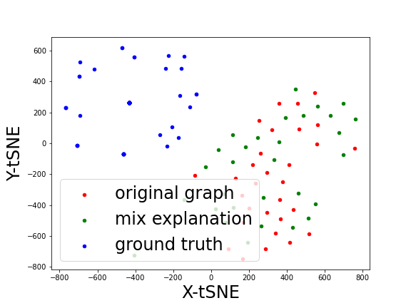
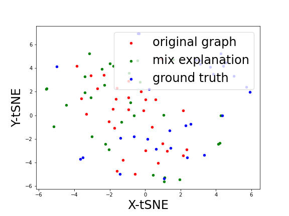
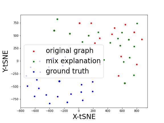
(a) BA-Shapes	(b) BA-Community	(c) Tree-Circles
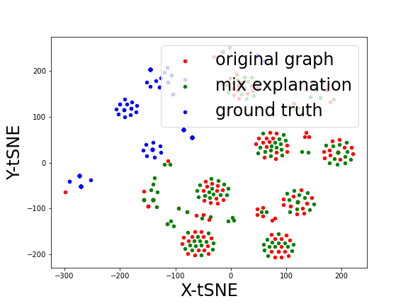
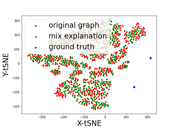
(d) Tree-Grid	(e) BA-2motifs	(f) MUTAG

Figure 4. Visualizations of the distribution shifting issue with t-SNE on six datasets. The points are generated with the output before the last layer of the model to be explained $f$, which is then plotted with t-SNE. The red points mean original graphs $G$, the blue points mean substructure explanations $G^{*}$, and the green points mean mixup explanations $G^{(mix)}$. Green dots align well with red dots, while blue dots shift away from red dots.

5.3. Alleviating Distribution Shifts (RQ2)

In the previous section, we showed that our MixUp approach outperforms existing explanation methods in terms of AUC-ROC. In this section, we show the existence of the distribution shifting issue and show our proposed mixup approach alleviates this issue and improves the performance in explanation w.r.t. AUC.

Visualizing Distributing Shifting. In this section, we show the existence of the distribution shifting issue by visualizing the distribution vector (the output of the last layer in a well-trained GNN model $f$) for the original graph $G$, the explanation from MixupExplainer $G^{(\text{mix})}$, and the ground truth explanation $G^{*}$ with t-Distributed Stochastic Neighbor Embedding(t-SNE) (Van der Maaten and Hinton, 2008). To calculate distribution vectors, we use the output of the last GNN layer in $f$ as the representation vector ${\bm{h}}$ for the original graph. Ground truth explanations $G^{*}$ and the mixup graph from MixupExplainer, $G^{(\text{mix})}$ are also fed into the model to achieve corresponding representations, denoted by ${\bm{h}}^{*}$, ${\bm{h}}^{(\text{mix})}$, respectively. The visualization results can be found in Figure 4. The red points represent the vectors from original graphs $\mathcal{G}$; the blue points represent vectors from substructure explanations $\mathcal{G}^{\prime}$, and the green points represent the vectors from the mixup explanations $\mathcal{G}^{\prime}_{mix}$. Note that for BA-2motifs, while there are multiple graphs in the dataset, with only two kinds of motifs as explanations, t-SNE only shows two blue points, which are actually multiple overlapping blue points. From Figure 4, we have the following observations:
 $\bullet$ The blue points shift away from the red points in most datasets, including both synthetic and real-world datasets. It means that the distribution shifting issue exists in most cases, where most existing work overlooked this issue.
 $\bullet$ The green points are inseparable from the red points in most datasets. It means that the explanation from MixupExplainer aligns well with the original graph’s distribution, which indicates our mixup approach’s effectiveness in alleviating the distribution shifting issue.
 $\bullet$ The shifting between blue points and red points is more obvious in the MUTAG dataset, where the green points generated by MixupExplainer still align well with the red points. This shows our method with mixup works well not only in synthetic datasets but also in the real-world dataset.

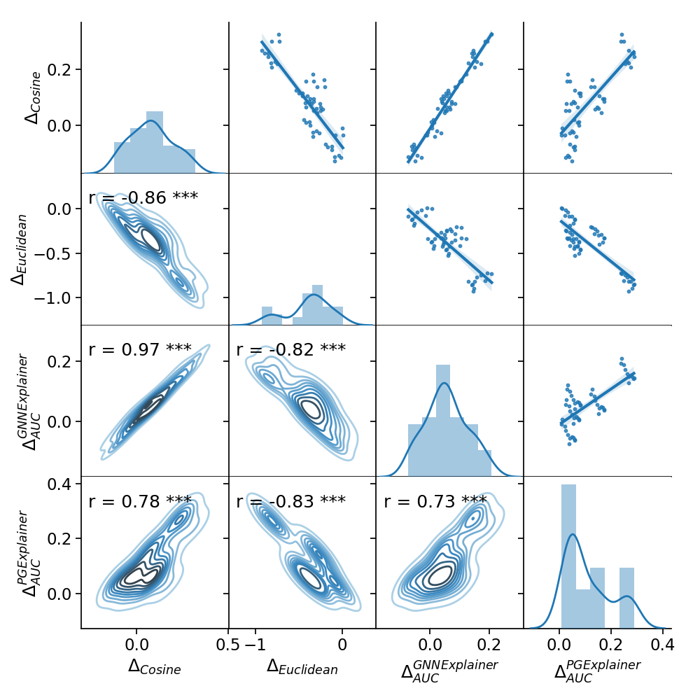
Figure 5. Correlation between improvements of AUC-ROC scores in explanation performance and the improvements of distribution distances on different datasets. The value of $r$ indicates the Pearson correlation coefficient, and the values with $*$ indicate statistical significance for correlation, where ^∗∗∗ indicates the p-value for testing non-correlation $p\leq 0.001$.

Measuring Distances. In this section, we quantitatively assess the distribution shifting issue by measuring the distances between the distribution vector ${\bm{h}}$ from the original graphs and the explanation subgraphs ${\bm{h}}^{*}$ and ${\bm{h}}^{(\text{mix})}$. We report the averaged Cosine score and the Euclidean distance between different types of representation vectors in Table 2. From the results, we can see that, on average, ${\bm{h}}^{(\text{mix})}$ has a higher Cosine score and a smaller Euclidean distance with ${\bm{h}}$ than ${\bm{h}}^{*}$, indicating more similarity of distribution between $G^{(\text{mix})}$ and $G$ than that between $G^{*}$ and $G$. The smaller distances between representation vectors demonstrate that our Mixup approach can effectively alleviate the distribution shifting problem caused by the inductive bias in the prediction model $f$. As $G^{(\text{mix})}$ better estimates the distribution of the original graphs, MixupExplainer can consistently improve the performance of existing explainers.

Correlation with Performance Improvements. We quantitatively evaluate the correlation between the improvements of AUC-ROC scores of MixupExplainer over basic counterparts and the improvements in distances with our mixup approach. We calculate the improvements of AUC-ROC scores from GNNExplainer and PGExplainer over GNNExplainer and PGExplainer without mixup (denoted as $\Delta_{\text{AUC}}^{\text{GNNExplainer}}$ and $\Delta_{\text{AUC}}^{\text{PGExplainer}}$, respectively). The improvements of average $\text{Cosine}({\bm{h}},{\bm{h}}^{(\text{mix})})$ over average $\text{Cosine}({\bm{h}},{\bm{h}}^{*})$ is denoted by $\Delta_{\text{Cosine}}$, and the improvements on Euclidean distance is $\Delta_{\text{Euclidean}}$. Figure 5 shows the correlation between $\Delta_{\text{AUC}}^{\text{GNNExplainer}}$, $\Delta_{\text{AUC}}^{\text{PGExplainer}}$, $\Delta_{\text{Cosine}}$, and $\Delta_{\text{Euclidean}}$. We can see that all these four improvements strongly correlated to each other with statistical significance, indicating the improvements achieved by MixupExplainer in explanations accuracy own to the successful alleviation of the distribution shifting issue.

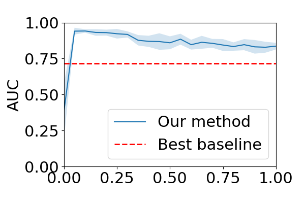
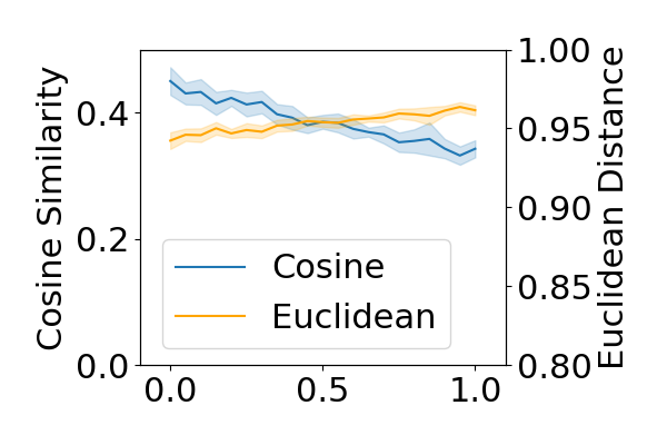
(a) AUC for different $\lambda$	(b) Distances for different $\lambda$

Figure 6. Hyper parameter analysis of $\lambda$ on BA-2motifs with Mixup-PGExplainer. (a) The performance of explanation w.r.t AUC. The blue line represents the mean AUC score with standard deviations over ten runs with different random seeds on each $\lambda$ value. The red line represents the performance of the baseline PGExplainer. (b) The distances between ${\bm{h}}$ and ${\bm{h}}^{(\text{mix})}$ for different $\lambda$. The blue and yellow lines represent the mean of the Cosine score and Euclidean distance with standard deviations, respectively.

5.4. Parameter Study (RQ3)

In this section, we investigate the hyperparameters of our approach, which include $\lambda$ and $\eta$, on the BA-2motifs dataset. The hyperparameter $\lambda$ controls the weight on the original graph during the mixup process. We find the optimal value of $\lambda$ by tuning it within the $[0,1]$ range. Note that, with $\lambda=0$, Eq. (7) is trivial and doesn’t help explain $G_{a}$ with only ${\bm{A}}_{b}$. The experimental results can be found in Figure 6. We can see that the best performance is achieved with $\lambda=0.1$ and that the approach consistently outperforms the best performance from baselines with $\lambda\in[0.05,1]$. The hyperparameter $\eta$ is the number of cross-graph edges during mixup, indicating the connectivity between label-dependent explanations and label-independent subgraphs. We tune it within the $[1,20]$ range on the BA-2motifs dataset. The results in Figure 7 show that the best performance is achieved with $\eta=1$. With different $\eta$, our approach shows stable and consistently better performance than the best baseline.

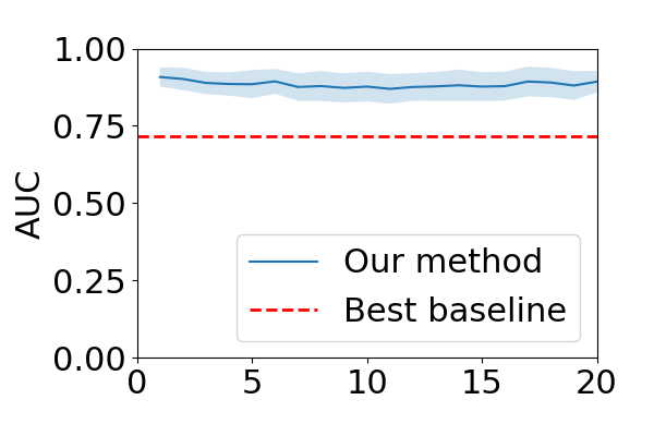
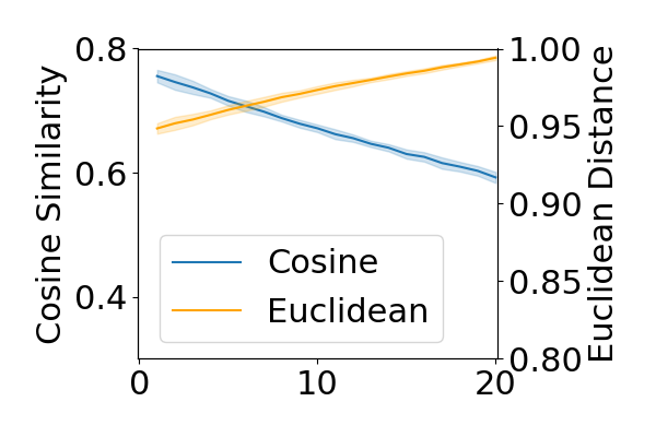
(a) AUC for different $\eta$	(b) Distances for different $\eta$

Figure 7. Hyperparameter analysis of $\eta$ on BA-2motifs with Mixup-PGExplainer. (a) The performance of explanation w.r.t AUC. (b) The distances between ${\bm{h}}$ and ${\bm{h}}^{(\text{mix})}$ for different $\eta$.

6. Conclusion

In this work, we study the distribution shifting problem to obtain robust explanations for GNNs, which is largely neglected by the existing GIB-based post-hoc instance-level explanation framework. With a close analysis of the explanation methods of GNNs, we emphasize the possible distribution shifting issue induced by the existing framework. We propose a simple yet effective approach to address the distribution shifting issue by mixing up the explanation with a randomly sampled base graph structure. The designed algorithms can be incorporated into existing methods with no effort. Experiments validate its effectiveness, and further theoretical analysis shows that it is more effective in alleviating the distribution shifting issue in graph explanation. In the future, we will seek more robust explanations. Increased robustness indicates stronger generality and could provide better class-level interpretation at the same time.

Appendix A APPENDIX

A.1. Graph Mixup Algorithm

Algorithm 1 Graph Mixup Algorithm

1:Graph $G_{a}=({\bm{X}}_{a},{\bm{A}}_{a})$, a set of graphs ${\mathcal{G}}$, the number of random connections $\eta$, explanation model $g$.

2:Graph $G^{(\text{mix})}$.

3:Randomly sample a graph $G_{b}=({\bm{A}}_{b},{\bm{X}}_{b})$ from ${\mathcal{G}}$

4:Generate mask matrix ${\bm{M}}_{a}=g(G_{a})$

5:Generate mask matrix ${\bm{M}}_{b}=g(G_{b})$

6:Sample $\eta$ random connections between $G_{a}$ and $G_{b}$ as ${\bm{A}}_{c}$

7:Mixup adjacency matrix ${\bm{A}}^{(\text{mix})}$ with Eq. (10)

8:Mixup edge mask ${\bm{M}}^{(\text{mix})}$ with Eq. (11)

9:Mixup node features ${\bm{X}}^{(\text{mix})}=[{\bm{X}}_{a};{\bm{X}}_{b}]$

10:return $G^{(\text{mix})}=({\bm{X}}^{(\text{mix})},{\bm{M}}^{(\text{mix})}\odot{\bm{A}}^{(\text{mix})})$

References

- (1)
- Atwood and Towsley (2016) James Atwood and Don Towsley. 2016. Diffusion-convolutional neural networks. Advances in neural information processing systems 29 (2016).
- Baldassarre and Azizpour (2019) Federico Baldassarre and Hossein Azizpour. 2019. Explainability Techniques for Graph Convolutional Networks.
- Balın et al. (2019) Muhammed Fatih Balın, Abubakar Abid, and James Zou. 2019. Concrete autoencoders: Differentiable feature selection and reconstruction. In International conference on machine learning. PMLR, 444–453.
- Bruna et al. (2013) Joan Bruna, Wojciech Zaremba, Arthur Szlam, and Yann LeCun. 2013. Spectral networks and locally connected networks on graphs. arXiv preprint arXiv:1312.6203 (2013).
- Chang et al. (2018) Chun-Hao Chang, Elliot Creager, Anna Goldenberg, and David Duvenaud. 2018. Explaining Image Classifiers by Counterfactual Generation. https://doi.org/10.48550/ARXIV.1807.08024
- Chereda et al. (2019) Hryhorii Chereda, Annalen Bleckmann, Frank Kramer, Andreas Leha, and Tim Beissbarth. 2019. Utilizing Molecular Network Information via Graph Convolutional Neural Networks to Predict Metastatic Event in Breast Cancer.. In GMDS. 181–186.
- Dai et al. (2022) Enyan Dai, Wei Jin, Hui Liu, and Suhang Wang. 2022. Towards robust graph neural networks for noisy graphs with sparse labels. In Proceedings of the Fifteenth ACM International Conference on Web Search and Data Mining. 181–191.
- Dai and Wang (2021) Enyan Dai and Suhang Wang. 2021. Towards Self-Explainable Graph Neural Network.
- Debnath et al. (1991) Asim Kumar Debnath, Rosa L Lopez de Compadre, Gargi Debnath, Alan J Shusterman, and Corwin Hansch. 1991. Structure-activity relationship of mutagenic aromatic and heteroaromatic nitro compounds. correlation with molecular orbital energies and hydrophobicity. Journal of medicinal chemistry 34, 2 (1991), 786–797.
- Duvenaud et al. (2015) David K Duvenaud, Dougal Maclaurin, Jorge Iparraguirre, Rafael Bombarell, Timothy Hirzel, Alán Aspuru-Guzik, and Ryan P Adams. 2015. Convolutional networks on graphs for learning molecular fingerprints. Advances in neural information processing systems 28 (2015).
- Fang et al. (2023) Junfeng Fang, Wei Liu, An Zhang, Xiang Wang, Xiangnan He, Kun Wang, and Tat-Seng Chua. 2023. On Regularization for Explaining Graph Neural Networks: An Information Theory Perspective. https://openreview.net/forum?id=5rX7M4wa2R_
- Feng et al. (2023) Zhiyuan Feng, Kai Qi, Bin Shi, Hao Mei, Qinghua Zheng, and Hua Wei. 2023. Deep evidential learning in diffusion convolutional recurrent neural network. , 2252-2264 pages.
- Guo and Mao (2021) Hongyu Guo and Yongyi Mao. 2021. ifmixup: Towards intrusion-free graph mixup for graph classification. arXiv e-prints (2021), arXiv–2110.
- Hamilton et al. (2017) Will Hamilton, Zhitao Ying, and Jure Leskovec. 2017. Inductive representation learning on large graphs. Advances in neural information processing systems 30 (2017).
- Han et al. (2022) Xiaotian Han, Zhimeng Jiang, Ninghao Liu, and Xia Hu. 2022. G-mixup: Graph data augmentation for graph classification. In International Conference on Machine Learning. PMLR, 8230–8248.
- Holdijk et al. (2021) Lars Holdijk, Maarten Boon, Stijn Henckens, and Lysander de Jong. 2021. [Re] Parameterized Explainer for Graph Neural Network. In ML Reproducibility Challenge 2020. https://openreview.net/forum?id=8JHrucviUf
- Kingma and Ba (2014) Diederik P Kingma and Jimmy Ba. 2014. Adam: A method for stochastic optimization. arXiv preprint arXiv:1412.6980 (2014).
- Kipf and Welling (2016) Thomas N Kipf and Max Welling. 2016. Semi-supervised classification with graph convolutional networks. arXiv preprint arXiv:1609.02907 (2016).
- Lei et al. (2022) Xiaoliang Lei, Hao Mei, Bin Shi, and Hua Wei. 2022. Modeling Network-level Traffic Flow Transitions on Sparse Data. In Proceedings of the 28th ACM SIGKDD Conference on Knowledge Discovery and Data Mining. 835–845.
- Li et al. (2017) Jundong Li, Kewei Cheng, Suhang Wang, Fred Morstatter, Robert P. Trevino, Jiliang Tang, and Huan Liu. 2017. Feature Selection: A Data Perspective. ACM Comput. Surv. 50, 6, Article 94 (dec 2017), 45 pages. https://doi.org/10.1145/3136625
- Li and Zhu (2021) Mengzhang Li and Zhanxing Zhu. 2021. Spatial-Temporal Fusion Graph Neural Networks for Traffic Flow Forecasting. Proceedings of the AAAI Conference on Artificial Intelligence 35, 5 (May 2021), 4189–4196.
- Li et al. (2022) Yiqiao Li, Jianlong Zhou, Sunny Verma, and Fang Chen. 2022. A survey of explainable graph neural networks: Taxonomy and evaluation metrics. arXiv preprint arXiv:2207.12599 (2022).
- Longa et al. (2022) Antonio Longa, Steve Azzolin, Gabriele Santin, Giulia Cencetti, Pietro Liò, Bruno Lepri, and Andrea Passerini. 2022. Explaining the Explainers in Graph Neural Networks: a Comparative Study. arXiv preprint arXiv:2210.15304 (2022).
- Luo et al. (2020) Dongsheng Luo, Wei Cheng, Dongkuan Xu, Wenchao Yu, Bo Zong, Haifeng Chen, and Xiang Zhang. 2020. Parameterized explainer for graph neural network. Advances in neural information processing systems 33 (2020), 19620–19631.
- Mansimov et al. (2019) E. Mansimov, O. Mahmood, and S. Kang. 2019. Molecular Geometry Prediction using a Deep Generative Graph Neural Network. https://doi.org/10.1038/s41598-019-56773-5
- Miao et al. (2022) Siqi Miao, Mia Liu, and Pan Li. 2022. Interpretable and generalizable graph learning via stochastic attention mechanism. In International Conference on Machine Learning. PMLR, 15524–15543.
- Min et al. (2021) Shengjie Min, Zhan Gao, Jing Peng, Liang Wang, Ke Qin, and Bo Fang. 2021. STGSN — A Spatial–Temporal Graph Neural Network framework for time-evolving social networks. Knowledge-Based Systems 214 (2021), 106746.
- Qiu et al. (2022) Luyu Qiu, Yi Yang, Caleb Chen Cao, Yueyuan Zheng, Hilary Ngai, Janet Hsiao, and Lei Chen. 2022. Generating Perturbation-Based Explanations with Robustness to Out-of-Distribution Data. In Proceedings of the ACM Web Conference 2022 (Virtual Event, Lyon, France) (WWW ’22). Association for Computing Machinery, New York, NY, USA, 3594–3605. https://doi.org/10.1145/3485447.3512254
- Scarselli et al. (2009) Franco Scarselli, Marco Gori, Ah Chung Tsoi, Markus Hagenbuchner, and Gabriele Monfardini. 2009. The Graph Neural Network Model. IEEE Transactions on Neural Networks 20, 1 (2009), 61–80.
- Shan et al. (2021a) Caihua Shan, Yifei Shen, Yao Zhang, Xiang Li, and Dongsheng Li. 2021a. Reinforcement Learning Enhanced Explainer for Graph Neural Networks. In Advances in Neural Information Processing Systems, M. Ranzato, A. Beygelzimer, Y. Dauphin, P.S. Liang, and J. Wortman Vaughan (Eds.), Vol. 34. Curran Associates, Inc., 22523–22533. https://proceedings.neurips.cc/paper/2021/file/be26abe76fb5c8a4921cf9d3e865b454-Paper.pdf
- Shan et al. (2021b) Caihua Shan, Yifei Shen, Yao Zhang, Xiang Li, and Dongsheng Li. 2021b. Reinforcement Learning Enhanced Explainer for Graph Neural Networks. In Advances in Neural Information Processing Systems, A. Beygelzimer, Y. Dauphin, P. Liang, and J. Wortman Vaughan (Eds.). https://openreview.net/forum?id=nUtLCcV24hL
- Sorokin and Gurevych (2018) Daniil Sorokin and Iryna Gurevych. 2018. Modeling Semantics with Gated Graph Neural Networks for Knowledge Base Question Answering. In Proceedings of the 27th International Conference on Computational Linguistics. Association for Computational Linguistics, Santa Fe, New Mexico, USA, 3306–3317. https://aclanthology.org/C18-1280
- Spinelli et al. (2022) Indro Spinelli, Simone Scardapane, and Aurelio Uncini. 2022. A meta-learning approach for training explainable graph neural networks. IEEE Transactions on Neural Networks and Learning Systems (2022).
- Tang et al. (2019) Shanshan Tang, Bo Li, and Haijun Yu. 2019. ChebNet: Efficient and stable constructions of deep neural networks with rectified power units using chebyshev approximations. arXiv preprint arXiv:1911.05467 (2019).
- Tishby et al. (2000) Naftali Tishby, Fernando C Pereira, and William Bialek. 2000. The information bottleneck method. arXiv preprint physics/0004057 (2000).
- Tishby and Zaslavsky (2015) Naftali Tishby and Noga Zaslavsky. 2015. Deep learning and the information bottleneck principle. In 2015 ieee information theory workshop (itw). IEEE, 1–5.
- Van der Maaten and Hinton (2008) Laurens Van der Maaten and Geoffrey Hinton. 2008. Visualizing data using t-SNE. Journal of machine learning research 9, 11 (2008).
- Veličković et al. (2017) Petar Veličković, Guillem Cucurull, Arantxa Casanova, Adriana Romero, Pietro Lio, and Yoshua Bengio. 2017. Graph attention networks. arXiv preprint arXiv:1710.10903 (2017).
- Verma et al. (2019) Vikas Verma, Alex Lamb, Christopher Beckham, Amir Najafi, Ioannis Mitliagkas, David Lopez-Paz, and Yoshua Bengio. 2019. Manifold mixup: Better representations by interpolating hidden states. In International conference on machine learning. PMLR, 6438–6447.
- Verma et al. (2021) Vikas Verma, Meng Qu, Kenji Kawaguchi, Alex Lamb, Yoshua Bengio, Juho Kannala, and Jian Tang. 2021. Graphmix: Improved training of gnns for semi-supervised learning. In Proceedings of the AAAI conference on artificial intelligence, Vol. 35. 10024–10032.
- Wang et al. (2020) Xiaoyang Wang, Yao Ma, Yiqi Wang, Wei Jin, Xin Wang, Jiliang Tang, Caiyan Jia, and Jian Yu. 2020. Traffic Flow Prediction via Spatial Temporal Graph Neural Network. In Proceedings of The Web Conference 2020 (Taipei, Taiwan) (WWW ’20). Association for Computing Machinery, New York, NY, USA, 1082–1092.
- Wang et al. (2021b) Xiang Wang, Yingxin Wu, An Zhang, Xiangnan He, and Tat-seng Chua. 2021b. Causal screening to interpret graph neural networks. (2021).
- Wang et al. (2021a) Yiwei Wang, Wei Wang, Yuxuan Liang, Yujun Cai, and Bryan Hooi. 2021a. Mixup for node and graph classification. In Proceedings of the Web Conference 2021. 3663–3674.
- Wu et al. (2022) Bingzhe Wu, Jintang Li, Junchi Yu, Yatao Bian, Hengtong Zhang, CHaochao Chen, Chengbin Hou, Guoji Fu, Liang Chen, Tingyang Xu, et al. 2022. A survey of trustworthy graph learning: Reliability, explainability, and privacy protection. arXiv preprint arXiv:2205.10014 (2022).
- Wu et al. (2021) Lirong Wu, Haitao Lin, Zhangyang Gao, Cheng Tan, Stan Li, et al. 2021. Graphmixup: Improving class-imbalanced node classification on graphs by self-supervised context prediction. arXiv preprint arXiv:2106.11133 (2021).
- Wu et al. (2020) Tailin Wu, Hongyu Ren, Pan Li, and Jure Leskovec. 2020. Graph information bottleneck. Advances in Neural Information Processing Systems 33 (2020), 20437–20448.
- Wu et al. (2019) Zonghan Wu, Shirui Pan, Guodong Long, Jing Jiang, and Chengqi Zhang. 2019. Graph Wavenet for Deep Spatial-Temporal Graph Modeling. In Proceedings of the 28th International Joint Conference on Artificial Intelligence (Macao, China) (IJCAI’19). AAAI Press, 1907–1913.
- Xiao et al. (2021) Teng Xiao, Zhengyu Chen, Donglin Wang, and Suhang Wang. 2021. Learning how to propagate messages in graph neural networks. In Proceedings of the 27th ACM SIGKDD Conference on Knowledge Discovery & Data Mining. 1894–1903.
- Yao et al. (2022) Huaxiu Yao, Yiping Wang, Linjun Zhang, James Zou, and Chelsea Finn. 2022. C-Mixup: Improving Generalization in Regression. arXiv preprint arXiv:2210.05775 (2022).
- Ying et al. (2019) Zhitao Ying, Dylan Bourgeois, Jiaxuan You, Marinka Zitnik, and Jure Leskovec. 2019. Gnnexplainer: Generating explanations for graph neural networks. Advances in neural information processing systems 32 (2019). https://doi.org/10.48550/ARXIV.1903.03894
- Yu et al. (2020) Junchi Yu, Tingyang Xu, Yu Rong, Yatao Bian, Junzhou Huang, and Ran He. 2020. Graph information bottleneck for subgraph recognition. arXiv preprint arXiv:2010.05563 (2020).
- Yuan et al. (2022) Hao Yuan, Haiyang Yu, Shurui Gui, and Shuiwang Ji. 2022. Explainability in graph neural networks: A taxonomic survey. IEEE Transactions on Pattern Analysis and Machine Intelligence (2022).
- Yuan et al. (2021) Hao Yuan, Haiyang Yu, Jie Wang, Kang Li, and Shuiwang Ji. 2021. On explainability of graph neural networks via subgraph explorations. In International Conference on Machine Learning. PMLR, 12241–12252.
- Zhang et al. (2017) Hongyi Zhang, Moustapha Cisse, Yann N. Dauphin, and David Lopez-Paz. 2017. mixup: Beyond Empirical Risk Minimization. https://doi.org/10.48550/ARXIV.1710.09412
- Zhang et al. (2022) He Zhang, Bang Wu, Xingliang Yuan, Shirui Pan, Hanghang Tong, and Jian Pei. 2022. Trustworthy graph neural networks: Aspects, methods and trends. arXiv preprint arXiv:2205.07424 (2022).
- Zhao et al. (2023) Tianxiang Zhao, Dongsheng Luo, Xiang Zhang, and Suhang Wang. 2023. Towards Faithful and Consistent Explanations for Graph Neural Networks. In WSDM.