This paper proposes a novel dynamic forecasting method using a new supervised Principal Component Analysis (PCA) when a large number of predictors are available. The new supervised PCA provides an effective way to bridge the gap between predictors and the target variable of interest by scaling and combining the predictors and their lagged values, resulting in an effective dynamic forecasting. Unlike the traditional diffusion-index approach, which does not learn the relationships between the predictors and the target variable before conducting PCA, we first re-scale each predictor according to their significance in forecasting the targeted variable in a dynamic fashion, and a PCA is then applied to a re-scaled and additive panel, which establishes a connection between the predictability of the PCA factors and the target variable. Furthermore, we also propose to use penalized methods such as the LASSO approach to select the significant factors that have superior predictive power over the others. Theoretically, we show that our estimators are consistent and outperform the traditional methods in prediction under some mild conditions. We conduct extensive simulations to verify that the proposed method produces satisfactory forecasting results and outperforms most of the existing methods using the traditional PCA. A real example of predicting U.S. macroeconomic variables using a large number of predictors showcases that our method fares better than most of the existing ones in applications. The proposed method thus provides a comprehensive and effective approach for dynamic forecasting in high-dimensional data analysis.

Keywords: Dynamic Forecasting, Factor Analysis, Supervised Principal Components, Large-Dimension, LASSO

JEL classification: C22, C23, C38, C53

1 Introduction

Dynamic forecasting is the process of analyzing time series data using statistical and dynamic modeling techniques to make predictions and to inform strategic decision-making. Recent advances in information technologies make it possible to collect large amounts of data over time, which naturally form high-dimensional time series and characterize many contemporary application problems in business, economics, finance, environmental sciences, and other scientific fields. Extracting useful information from such high-dimensional dependent data to make accurate predictions, dimension reduction becomes a necessity. In the past decades, there have been many dimension-reduction methods developed in the literature, and one of the most successful ones is the Principal Component Analysis (PCA). The PCA method is a versatile tool for dimension reduction and is capable of extracting useful features by transforming the observed variables into a few new uncorrelated factors while retaining much information in the data. See Anderson (1958) and Anderson (1963) for its basic concept and properties. The PCA has many applications in various scientific areas, including business, economics, finance, and management. An incomplete list of recent works includes the asset pricing in Gu, Kelly, and Xiu (2020), Giglio and Xiu (2021), and He, Huang, Li, and Zhou (2022), the econometric modeling and forecasting in Mullainathan and Spiess (2017), Gao and Tsay (2022), and Huang, Jiang, Li, Tong, and Zhou (2022), the business and management in Kim, Street, Russell, and Menczer (2005), among others. Despite its importance, existing works in these fields mainly focus on employing a static decomposition, where the extracted principal components represent the cross-sectional structure of a contemporaneous panel and ignore the information embedded in the past lagged variables of the series.

Arguably the most widely used forecasting method that relies on PCA is the “diffusion-index” approach, which is also known as factor-augmented model developed by Stock and Watson (2002a, b) and has received much attention among researchers and practitioners. In a data-rich environment, it has become common that the number of predictors is large and may exceed the number of data points. The factor-based diffusion-index approach is widely applicable under such situations. Specifically, for a high-dimensional observed predictor vector ${\mathbf{x}}_{t}\in R^{N}$, the goal is to predict $y_{t+h}$ based on the available information $\{{\mathbf{x}}_{j},j=1,...,t\}$. To avoid the curse of dimensionality, the factor-based approach assumes that the predictors and the variable of interest admit the following structure:

$$\begin{array}[]{c}{\mathbf{x}}_{t}={\mathbf{B}}{\mathbf{f}}_{t}+{\mathbf{u}}_{t},\\ y_{t+h}=\boldsymbol{\beta}^{\prime}{\mathbf{f}}_{t}+\mbox{\boldmath$\varepsilon$}_{t+h},\end{array}$$ (1)

where ${\mathbf{x}}_{t}$ and $y_{t}$ are both taken to have mean zero, ${\mathbf{f}}_{t}$ is an $r$-dimensional vector of latent factors, which may also contain the dynamic factors in Stock and Watson (2002a, b), ${\mathbf{B}}$ is the associated factor loading matrix, ${\mathbf{u}}_{t}$ is an $N$-dimensional idiosyncratic term, which is uncorrelated with the factors ${\mathbf{f}}_{t}$, and $\boldsymbol{\beta}$ is an $r$-dimensional slope parameter linking the factors ${\mathbf{f}}_{t}$ to $y_{t+h}$ with $h>0$.

Motivated by the success of the diffusion-index approach and to explore further available information in ${\mathbf{x}}_{t}$ for predicting $y_{t+h}$, we consider the following four perspectives to develop the proposed approach:

1. Information perspective: Because of the serial dependence in time-series data, past lagged variables of ${\mathbf{x}}_{t}$ are often helpful in predicting $y_{t+h}$. For example, the lagged variables are used in a factor-augmented VAR model in Bernanke, Boivin, and Eliasz (2005) for studying the effect of monetary policy on the economy. Yet there is no unified approach available under the existing methods to incorporating lagged information. Different users make use of the lagged variables in different ways. Consider the diffusion approach. One can augment lagged values of the predictors to form an extended predictor vector before applying PCA to extract common factors. The extracted factors are then linear combinations of ${\mathbf{x}}_{t}$ and its lagged variables. Another possibility is to use lagged values of the extracted factors obtained from the original predictors. This procedure assumes a priori that the linear combinations of predictors carry over lags. Consequently, the lagged information is exploited differently and there are no guidelines available to best use the lagged variables. In addition, there is no simple way to select the number of past lagged variables needed in an application.

2. Adaptive perspective: Empirical applications are often interested in both short-term and long-term predictions so that various choices of $h$ in Model (1) are employed. Yet the same common factors are used for all choices of $h$ because an unsupervised PCA does not consider the target variable in extracting common factors. It is possible in applications that useful predictors for $y_{t+h}$ may not be good ones for $y_{t+h^{\prime}}$ under the setting in Model (1), where $h\neq h^{\prime}$.

3. Supervision perspective: In machine learning, applying principal component analysis to extract the latent factors from ${\mathbf{x}}_{t}$ is an unsupervised procedure. It does not require any information of the target variable $y_{t+h}$. This might become a drawback in prediction as the target variable is of main interest. In addition, PCA is not scale-invariant, and the extracted factors can change easily when scales of the components of ${\mathbf{x}}_{t}$ change. This may lead to inferior prediction if care is not exercised in applying diffusion index models. For this reason, the components of ${\mathbf{x}}_{t}$ are often standardized before applying PCA.

4. Accuracy in factor extraction: The traditional PCA method may not provide accurate estimation of the common factors, especially when some common factors are strong and the remaining ones are weak; see, for example, the explanation in Huang, Jiang, Li, Tong, and Zhou (2022) and Bai and Ng (2023). For time series data, common factors that have stronger serial dependence tend to dominate those with weaker serial dependence as strong serial dependence often results in higher variances, which in turn leads to larger eigenvalues in the covariance matrix of ${\mathbf{x}}_{t}$.

In view of the above discussions, we propose a new diffusion-index model in this paper for dynamic forecasting by developing a supervised dynamic PCA (sdPCA) method. First, our proposed sdPCA takes explicitly the lagged variables of predictors into account. Each predictor is allowed to have its own number of past lagged variables. In fact, the number of lagged variables for each predictor may be selected by an information criterion function such as the Akaike Information Criterion. Second, our new diffusion-index model can also employ lagged variables of the extracted common factors. Therefore, the proposed approach explores the dynamic dependence in two ways. The extracted factors by the proposed sdPCA contain lagged variables of the predictors and the new diffusion-index model also employs lagged variables of the common factors. Consequently, our new approach is different from the settings in Stock and Watson (2002a) and in Bai and Ng (2006), where, as discussed earlier, the lagged dependence is not fully explored. Third, our sdPCA incorporates information of the target variable $y_{t+h}$ in constructing the predictor vector for PCA so that the scale of each component of the predictor vector is properly adjusted. Consequently, the proposed new approach does not depend on the scales of observed predictor ${\mathbf{x}}_{t}$. This property is similar to that of the sPCA of Huang, Jiang, Li, Tong, and Zhou (2022). Fourth, the sdPCA is adaptive in extracting common factors so that the common factors used to predict $y_{t+h}$ and $y_{t+h^{\prime}}$ may be different. This can enhance the predictive power of the proposed new diffusion-index model.

There are two steps in the proposed sdPCA that produces useful factors to serve as predictors. First, sdPCA runs predictive linear regressions of the target variable on each observed predictor and its past lagged variables with the number of lags being selected by an information criterion. In this way, useful lagged variables of each predictor are properly addressed. The fitted values of the individual predictive linear regressions form a new high-dimensional predictor vector on which PCA is carried out to extract common factors. Since the predictive linear regression automatically adjusts the scale of each predictor, the scaling effect of observed predictors on PCA is also properly addressed. As a matter of fact, one can think of the scale of each predictor being adjusted based on its predictive power to the target variable. This adjustment may depend on $h$, the number of step ahead prediction of interest. Second, sdPCA allows users to add lagged variables of extracted factors to the contemporaneous ones in the linear prediction model. This enables us to explore farther the dynamic information of the data to improve the forecasts. A similar technique is discussed in Stock and Watson (2002b) under different settings. In short, these two steps of the proposed sdPCA not only capture the dynamic information of the data in an additive manner, but also adjust automatically the scaling effect of the data. More importantly, the steps enable users to explore fully the linear dependence of the data to improve the accuracy of prediction. We show that, under some general conditions, the proposed sdPCA can outperform the traditional diffusion-index approach using unsupervised PCA, both in theory and in simulation.

Asymptotic properties of the proposed sdPCA are established under the modern setting that the number of predictors $N$ and the sample size $T$ diverge to infinity. We also compare the proposed method with some commonly used methods, and derive the conditions under which, the proposed method can outperform the existing ones theoretically. In addition, to embrace the modern development of machine learning techniques, we also apply the well-known least absolute shrinkage and selection operator (Lasso) approach to select the most relevant factors that have predictive power for the target variable. Theoretically, we also establish the consistency of the Lasso estimators under some identification conditions.

We illustrate and assess the performance of the proposed sdPCA and the new diffusion-index forecasting method with an application to macroeconomic index forecasting. We forecast the U.S. industrial production (IP) growth, change in the unemployment rate (UNRATE), the consumer price index: all (CPI-All), the S&P 500 index volatility change (Volatility Change), and the S&P 500 index return using 123 macroeconomic variables from FRED-MD, as that in Huang, Jiang, Li, Tong, and Zhou (2022), McCracken and Ng (2016), Stock and Watson (2002a, b), among others. Similarly to those in Huang, Jiang, Li, Tong, and Zhou (2022), the sdPCA loadings have re-assigned the weights to the predictors and a smaller subset of the macro variables tend to have more predictive power compared with the unsupervised PCA loadings. Furthermore, the proposed sdPCA together with the Lasso procedure produces comparable or even better forecasting results compared with some commonly used factor-based forecasting methods, such as the traditional PCA method, the sPCA in Huang, Jiang, Li, Tong, and Zhou (2022), and the diffusion-index model in Stock and Watson (2002a, b).

The scaled PCA (sPCA) of Huang, Jiang, Li, Tong, and Zhou (2022) is the closest method to ours. Both methods reconstruct a new high-dimensional prediction vector before extracting common factors using PCA. However, our method differs from the sPCA in three ways. First, our proposed diffusion-index forecasts may include lagged variables of common factors as predictors while sPCA only uses the contemporaneous one. Thus, the predictive model in Huang, Jiang, Li, Tong, and Zhou (2022) is similar to that in Stock and Watson (2002a) whereas ours generalizes the traditional method to a dynamic fashion. As a matter of fact, sPCA is a special case of the sdPCA if one does not include any lagged variables of each predictor in constructing the high-dimensional prediction vector, nor use any lagged variables of the extracted factors. Second, instead of running simple linear regression of the target variable on each predictor alone, we run a time series regression by including lagged variables of the predictors with the number of lags being selected by an information criterion. In other words, the proposed sdPCA explores the dynamic dependence of the target variable on each observed predictor in constructing the new high-dimensional predictor vector for PCA. Third, the proposed prediction model uses the Lasso method to select the factors that have significant predictive power in prediction. This provides a data-driven approach to identifying relevant predictors.

There are other related works in the literature concerning supervised learning or building connections between predictors and the target variable in prediction; see the references in Huang, Jiang, Li, Tong, and Zhou (2022). We briefly discuss some differences between the proposed sdPCA approach and some related methods. Bai and Ng (2008) first applied a screening method to select a subset of predictors that are tested to have relatively more predictive power to the target under either soft- or hard-thresholding rules, and the PCA is conducted on the selected subset to extract common factors for use in the diffusion-index forecasting. Our proposed method, on the other hand, assigns different weights to each predictor and its lagged variables according to their predictive power without using any thresholding rule. An incomplete list of other related works that share similar insights to ours includes the partial least squares (PLS) regression in Wold (1966) and Kelly and Pruitt (2015) with financial applications in Kelly and Pruitt (2013), Huang, Jiang, Tu, and Zhou (2015), and Light, Maslov, and Rytchkov (2017), among others. The comparison of the aforementioned methods and the sPCA has been extensively studied in Huang, Jiang, Li, Tong, and Zhou (2022), and the sPCA is shown to have advantages in forecasting. Therefore, we only compare our proposed method with the sPCA and some commonly used factor-based linear forecasting methods in this paper.

The rest of the paper is organized as follows. Section 2 introduces the sdPCA method and the new diffusion-index model, and presents their asymptotic properties and some comparison results. Section 3 studies the finite-sample performance of the proposed approach via simulation, and 4 illustrates the proposed procedure with an empirical application. Section 5 concludes. All the proofs and derivations for the asymptotic results are relegated to an online Appendix.

Notation: We use the following notation. For a $p\times 1$ vector ${\mathbf{u}}=(u_{1},...,u_{p})^{\prime}$, $\|{\mathbf{u}}\|_{1}=\sum_{i=1}^{p}|u_{i}|$ is the $\ell_{1}$-norm and $\|{\mathbf{u}}\|_{\infty}=\max_{1\leq i\leq p}|u_{i}|$ is the $\ell_{\infty}$-norm. ${\mathbf{I}}_{p}$ denotes the $p\times p$ identity matrix. For a matrix ${\mathbf{H}}$, its Frobenius norm is $\|{\mathbf{H}}\|=[\mathrm{trace}({\mathbf{H}}^{\prime}{\mathbf{H}})]^{1/2}$ and its operator norm is $\|{\mathbf{H}}\|_{2}=\sqrt{\lambda_{\max}({\mathbf{H}}^{\prime}{\mathbf{H}})}$, where $\lambda_{\max}(\cdot)$ denotes the largest eigenvalue of a matrix, and $\|{\mathbf{H}}\|_{\min}$ is the square root of the minimum non-zero eigenvalue of ${\mathbf{H}}{\mathbf{H}}^{\prime}$. The superscript ^′ denotes the transpose of a vector or matrix. We also use the notation $a\asymp b$ to denote $a=O(b)$ and $b=O(a)$.

2 Methodology

2.1 Model Setup

Let ${\mathbf{x}}_{t}=(x_{1,t},...,x_{N,t})^{\prime}$ be an $N$-dimensional observable time series, for $t=1,...,T$, and $y_{t+h}$ be the target variable of interest, where $h\geq 1$. The goal is to predict $y_{t+h}$ using ${\mathbf{x}}_{t}$ and its past information. Based on the discussion in the Introduction section, we assume the data are centered and consider the following model:

$$\begin{array}[]{c}{\mathbf{x}}_{t}={\mathbf{B}}{\mathbf{f}}_{t}+{\mathbf{u}}_{t},\\ y_{t+h}=\boldsymbol{\beta}(L)^{\prime}{\mathbf{f}}_{t}+{\varepsilon}_{t+h},\end{array}$$ (2)

where $\boldsymbol{\beta}(L)=\boldsymbol{\beta}_{0}+\boldsymbol{\beta}_{1}L+...+\boldsymbol{\beta}_{q-1}L^{q-1}$ with $L$ being the backshift (or lag) operator such that $L{\mathbf{f}}_{t}={\mathbf{f}}_{t-1}$, and $q\geq 1$ is the number of lagged variables of factors used in predictions. When $q=1$, Model (2) reduces to the diffusion-index forecasting equation in (1).

The model in (2) is similar to that in Stock and Watson (2002a) and Bai and Ng (2006), but the mechanisms to produce predictions of the models are fundamentally different. In Stock and Watson (2002a), a dynamic factor model is considered for a large panel of time series and some dynamic factors are used as predictors, which are assumed to explain most of the variability of the panel, measured by the covariance matrix of the panel. Their factors not necessarily contain information of the past lagged values of ${\mathbf{x}}_{t}$. In Model (2), the observed time series ${\mathbf{x}}_{t}$ admits a factor structure with static factor processes, and these static factors and their past lagged variables are used as predictors in the prediction equation. For similar reasons, Model (2) is also different from the setting in Bai and Ng (2006) and Huang, Jiang, Li, Tong, and Zhou (2022). On the other hand, there are some similar insights between Model (2) and Model (2.3) in Stock and Watson (2002b) because both models attempt to explore the dynamic dependence of the data in the prediction. But the proposed model includes past lagged variables of the common factors whereas the one in Stock and Watson (2002b) employs the past lagged variables of $y_{t}$ in the prediction. A recursive expansion of $y_{t}$ in Model (2.3) of Stock and Watson (2002b) also leads to using past lagged variables of common factors as predictors albeit with some constraints in the coefficient parameters. For simplicity, we only consider Model (2) in this paper and investigate its predictive ability.

Under some identification conditions, it is natural to apply PCA to extract common factors from ${\mathbf{x}}_{t}$ and use the extracted factors and their lagged variables as predictors in predicting $y_{t+h}$. Alternatively, one may perform PCA on a stacked vector $({\mathbf{x}}_{t}^{\prime},{\mathbf{x}}_{t-1}^{\prime},...,{\mathbf{x}}_{t-q+1}^{\prime})^{\prime}$ and apply the extracted factors directly in forecasting. Since the factors so obtained already include the lagged variables of ${\mathbf{x}}_{t}$ so that no lagged variables of the factors are used. However, there are some drawbacks of this approach. First, the application of PCA in the first step does not learn any information from the target variable $y_{t+h}$ and, therefore, the factors extracted directly from the stacked vector may not have the best predictability for $y_{t+h}$. Second, the consistency of the PCA procedure is usually shown under the assumption of strong factors in the literature; see, for example, Bai and Ng (2002) and Fan, Liao, and Mincheva (2013). In practice, there is no guarantee that all the factors are strong because the noise effect can be prominent when adding more variables to ${\mathbf{x}}_{t}$. As a result, the factors extracted from all the components of ${\mathbf{x}}_{t}$ (or stacked vector) may not have better predictability than those from a subset of the panel. See Boivin and Ng (2006) for further information.

To overcome these drawbacks, we introduce a new supervised dynamic PCA method to extract the common factors and to employ relatively informative factors in a three-stage procedure to explore the dynamic dependence in the data. Our goal is to extract the factors that have more predictive power by learning from the target variable. In other words, we need to estimate the factors ${\mathbf{f}}_{t}$ using a new approach for predictions. Details are discussed next.

2.2 Estimation Procedure

In this section, we propose a new PCA useful for dynamic forecasting. The procedure consists of the following three steps:

1. For $i=1,...,N$, estimate the slope parameters by regressing the target variable on the $i$-th predictor and its past lagged variables:

   $$y_{t+h}\approx\widehat{\mu}_{i}+\widehat{\gamma}_{i,0}x_{i,t}+\widehat{\gamma}_{i,1}x_{i,t-1}+...+\widehat{\gamma}_{i,q_{i}-1}x_{i,t-q_{i}+1},\,\,t=q_{i},...,T-h,$$ (3)

   where $q_{i}$ is selected by an information criterion such as the Akaike Information Criterion (AIC). Let $q=\max_{1\leq i\leq N}\{q_{i}\}$.

2. For $t=q,q+1,...,T$, let $\widehat{\mathbf{x}}_{t}=(\widehat{x}_{1,t},...,\widehat{x}_{N,t})^{\prime}$ with $\widehat{x}_{i,t}=\widehat{\gamma}_{i,0}x_{i,t}+\widehat{\gamma}_{i,1}x_{i,t-1}+...+\widehat{\gamma}_{i,q_{i}-1}x_{i,t-q_{i}+1}$. Apply PCA to $\widehat{\mathbf{x}}_{t}$ and obtain the estimated factors $\widehat{\mathbf{g}}_{t}$, which contains the information of the original factors ${\mathbf{f}}_{t}$ as well as its lagged variables relevant to $y_{t+h}$. One can think of $\widehat{\mathbf{g}}_{t}$ as an estimator for $({\mathbf{f}}_{t}^{\prime},...,{\mathbf{f}}_{t-q+1}^{\prime})^{\prime}$ in Model (2) under some proper conditions.

3. For $t=q,q+1,...,T-h$, apply the Ordinary Least-Squares method to the linear regression of the target variable on $\widehat{\mathbf{g}}_{t}$ and obtain the estimated coefficients:

   $$y_{t+h}\approx\widehat{\alpha}+\widehat{\boldsymbol{\beta}}^{\prime}\widehat{\mathbf{g}}_{t},\,\,t=q,...,T-h.$$ (4)

   Finally, the prediction of $y_{T+h}$ is given by $\widehat{y}_{T+h}=\widehat{\alpha}+\widehat{\boldsymbol{\beta}}^{\prime}\widehat{\mathbf{g}}_{T}$.

Note that the intercepts $\widehat{\mu}_{i}$ and $\widehat{\alpha}$ in Step 1 and Step 3 above will be removed if the data are assumed to be centered as that in Model (2). Some remarks are as follows. First, the idea of learning from the target variable using linear regression is similar to that in Huang, Jiang, Li, Tong, and Zhou (2022). However, we focus on dynamic forecasting with lagged variables in the regression, while the sPCA of the aforementioned paper only uses contemporaneous information. Second, unlike the traditional method, the number of lagged variables of each observed predictor used in prediction is selected during the first step. Once the additive panel is formed according to the regression results in Step 1, the extracted factors in Step 2 will automatically contain the dynamic information and can be used as predictors in Step 3, which captures the dynamic dependence in time series forecasting. Third, we only use $\widehat{\mathbf{g}}_{t}$ in Step 3, but we can also employ some of its lagged variables if necessary. Furthermore, as will be seen in the next section, we apply Lasso regularization to obtain $\widehat{\boldsymbol{\beta}}$ so that adding additional lagged variables of $\widehat{\mathbf{g}}_{t}$ does not cause any difficulties to the proposed procedure. Fourth, when the number of predictors $N$ and the sample size $T$ are large, one can use a sufficiently large value $q$ in lieu of $q_{i}$ in Step 1 to simplify the computation.

2.3 When Diffusion-Index Forecast Meets Sparsity

As discussed before, even though we have constructed an $N$-dimensional vector of predictors in Step 2, it is possible that only a subset of the extracted common factors has predictive power for the target variable. Similar insights are also mentioned in Huang, Jiang, Li, Tong, and Zhou (2022), but a statistical approach to automatically select the significant factors is still not available therein.

In this section, we propose to use penalized regression methods to select the factors that have predictive power for the target variable. For simplicity, we assume the intercepts are zero and only introduce the Lasso approach since other penalized methods can be similarly established. Let $\widehat{\boldsymbol{\beta}}_{lasso}$ be the Lasso solution that solves the following optimization problem:

$$\widehat{\boldsymbol{\beta}}_{lasso}=\arg\min_{\boldsymbol{\beta}\in R^{rq}}\left\{\frac{1}{T}\sum_{t=q}^{T-h}\|y_{t+h}-\boldsymbol{\beta}^{\prime}\widehat{\mathbf{g}}_{t}\|^{2}+\lambda_{T}\|\boldsymbol{\beta}\|_{1}\right\},$$ (5)

where $\widehat{\mathbf{g}}_{t}$ is the extracted factor process from Step 2 of the proposed procedure in Section 2.2, and $\lambda_{T}>0$ is a penalty parameter to be determined later. The above optimization is a convex one and can be solved by many existing algorithms. See Hastie, Tibshirani, and Friedman (2009) for detailed illustrations.

The basic idea of using regularization estimation, such as the Lasso regression, is that possibly only a subset of $\widehat{\mathbf{g}}_{t}$ has predictive power for $y_{t+h}$. This is particularly so if $N$ is large. In this case, $\boldsymbol{\beta}$ is a sparse vector with only a few non-zero elements. The penalty parameter $\lambda_{T}$ is used to control the number of significant factors to be used in the predictions.

It is natural to ask why the proposed sdPCA and the new diffusion-index forecasts can outperform the traditional PCA and the scaled PCA in Huang, Jiang, Li, Tong, and Zhou (2022) in prediction. There are several reasons that can answer this question. First, consider the information aspect. Our proposed sdPCA generalizes the scaled PCA by including more relevant lagged variables of observed predictors. As such, the scaled PCA is a special case of the proposed method with $q_{i}=1$ at Step 1, for $i=1,\ldots,N$. Consequently, the proposed sdPCA captures more dynamic dependence information in the data and, hence, can improve the forecasting performance. Second, the proposed Lasso regression can further screen out irrelevant predictors, which in turn can improve parameter estimation and avoid the difficulty of over-parameterization, especially when $N$ is large.

Remark 1.

The Lasso procedure could be very helpful in practice because we do not know how many factors should be included as predictors in Step 3 of Section 2.2. Note that $\widehat{\mathbf{g}}_{t}$ in Step 3 can be treated as a proxy for $({\mathbf{f}}_{t}^{\prime},...,{\mathbf{f}}_{t-q+1}^{\prime})^{\prime}$, which contains the dynamic information learned by regressing the target variable on lagged predictors in Step-1 of the proposed procedure. In fact, we may also add the lagged variables of $\widehat{\mathbf{g}}_{t}$ and adopt Lasso to select the significant factors in prediction. This expanded approach can collect additional dynamic information that may be missed in Step 1. We do not explore any further this approach to save space.

Remark 2.

It is well-known that the Lasso estimate $\widehat{\boldsymbol{\beta}}_{lasso}$ is a biased estimate of the true coefficient $\boldsymbol{\beta}$. To correct the bias, one can re-run the linear regression using only those predictors selected by the Lasso procedure. This is referred to as a post-selection inference in the literature; see, for instance, Bellono and Cherozhukov (2013).

2.4 Selection of the Lag Parameters

We use information criteria in Step 1 of the proposed procedure to select the number $q_{i}$ of lagged variables for the predictor $x_{it}$; see Equation (3). In applying any information criterion, there is a need to select the maximum order allowed. This maximum order is unknown in practice, but there are statistical methods available to guide the choice. We mention two possibilities in this section. First, from a time series analysis point of view, the maximum order provides an approximation to the true lagged linear dependence between the target $y_{t+h}$ and $\{x_{it},x_{i,t-1},x_{i,t-2},\ldots\}$. When the sample size $T$ is large, one can improve the accuracy in approximation by increasing the maximum order allowed. Therefore, a common practice in the literature is to use $q_{max}\approx\log(T)$. In this way, the information criterion used selects $q_{i}\in[1,\ldots,q_{max}]$. This approach can also be applied to the selection of $q$ in the diffusion-index forecasting model of Step 3.

A second method is cross-validation, which is particularly useful when $N$ and $T$ are both large. We partition the data into two sub-samples, say $\{{\mathbf{x}}_{1},...,{\mathbf{x}}_{T_{1}-h},y_{h},...,y_{T_{1}}\}$ and $\{{\mathbf{x}}_{T_{1}-h+1},...,{\mathbf{x}}_{T-h},y_{T_{1}+1},...,y_{T}\}$ for some $T_{1}<T$. For a small integer $q_{max}\geq 1$ and each $1\leq q\leq q_{max}$, we perform the proposed estimation of Section 2.2 to the first sub-sample with $q_{i}=q$, for all $i$, and predict $y_{T_{1}+h}$ to compute the associated forecasting error. We then move the data $\{{\mathbf{x}}_{T_{1}-h+1},y_{T_{1}+1}\}$ from the second sub-sample to the first one and repeat the above procedure to calculate another forecasting error. This estimation-forecasting exercise is repeated until we obtain the forecast error of $y_{T}$. Then $\widehat{q}$ is chosen as the one that produces the smallest out-of-sample forecasting errors, where we may adopt the mean-squared forecasting error (RMSE) defined in (7) in Section 2.7 below.

Remark 3.

In the empirical study of macroeconomic forecasting, we adopt the second approach mentioned above because the number of predictors is large, and many macroeconomic indicators only depend on a small number of the most recent lagged variables. The AIC or BIC criterion can be treated as another option if one wants to further improve the forecasting accuracy of some variables of interest, though information criteria may not always outperform cross-validation in lag selection.

2.5 Selection of the Number of Factors

The above analysis depends on a known number of factors $r$, which is unknown in practice. As discussed in Bai and Ng (2023), if we want to estimate the number of factors with $\nu>0$, where $\nu$ is a strength parameter defined in Assumption 3 below, the criteria in Bai and Ng (2002) remain useful. In addition, there are other estimation methods such as the criteria of Onatski (2010) and Ahn and Horenstein (2013) which separate the bounded eigenvalues from diverging ones of the covariance matrix. For time series factor models with weak factors, Lam and Yao (2012) proposed a multi-step eigenvalue-ratio method to estimate the number of factors with different strengths. This method remains valid under our framework and it is especially useful when the factors have different strengths of weaknesses. Therefore, we may apply those existing methods to estimate the number of factors. Note that it might be helpful to include more factors as predictors and let the Lasso procedure select the factors that have more predictive power. Limited simulation results suggest that the Lasso method can accurately identify the number of significant factors.

We mention that there is an extreme case that the loading matrix associated with ${\mathbf{g}}_{t}$ in Step 2 may not be of full rank when $\boldsymbol{\beta}_{i}=\boldsymbol{\beta}_{j}$ for some $0\leq i,j\leq q-1$. Then the number of factors identified by the aforementioned methods would be fewer than the true one. But this is not an issue because we can treat ${\mathbf{f}}_{i,t}+{\mathbf{f}}_{j,t}$ as a new factor with components sharing a common regression coefficient in the linear forecasting step via a regression method. Simulation results in Section 3 suggest that the proposed method still works well in out-of-sample prediction.

Remark 4.

It is natural that the information criterion in Bai and Ng (2002) should be refined to cover the case of weak factors. However, a valid criterion depends on an accurate estimation of the strength parameter $\nu$ in Assumption 3 below, which is difficult to obtain in practice. This difficulty can be addressed by the Lasso procedure introduced in Section 2.3. Specifically, we adopt a data-driven procedure by including more factors as predictors in our empirical studies. The Lasso procedure can then select the factors that play important roles in forecasting the target variable.

2.6 Assumptions

In this section, we introduce the assumptions needed to derive theoretical results of the asymptotic forecasting performance of the proposed method. Most assumptions below are commonly used in the PCA or approximate-factor modeling literature, and the derivation of the consistency of the LASSO estimates needs some slightly stronger assumptions. We use $c$ or $C$ to denote a generic positive constant the value of which may change at different places.

Assumption 1.

The process $\{{\mathbf{f}}_{t}\}$ is $\alpha$-mixing with the mixing coefficients satisfying the condition $\alpha_{N}(k)<\exp(-k)$, where $\alpha_{N}(k)$ is defined as

$$\alpha_{N}(k)=\sup_{i}\sup_{A\in\mathcal{F}_{-\infty}^{i},B\in\mathcal{F}_{i+k}^{\infty}}|P(A\cap B)-P(A)P(B)|,$$ (6)

where $\mathcal{F}_{i}^{j}$ is the $\sigma$-field generated by $\{{\mathbf{f}}_{t}:i\leq t\leq j\}$.

Assumption 2.

For ${\mathbf{g}}_{t}=({\mathbf{f}}_{t}^{\prime},{\mathbf{f}}_{t-1}^{\prime},...,{\mathbf{f}}_{t-q+1}^{\prime})^{\prime}$ with a fixed $q\geq 1$, $\sup_{t}E\|{\mathbf{g}}_{t}\|^{4}\leq C$ and $\frac{1}{T}\sum_{t=q}^{T-h}{\mathbf{g}}_{t}{\mathbf{g}}_{t}^{\prime}\rightarrow_{p}\boldsymbol{\Sigma}_{g}$, which is a $qr\times qr$ positive-definite matrix.

Note that the $i$-th row of loading ${\mathbf{b}}_{i}$ can be either a random or a fixed constant vector. Either way, we may define ${\mathbf{b}}_{i}={\bf 0}$ symbolically if $x_{i,t}$ does not depend on the common factors. Thus, ${\mathbf{b}}_{i}\neq{\bf 0}$ implies that $x_{i,t}$ depends on the common factors with some positive probability. We define $\mathcal{I}_{b}=\{i:{\mathbf{b}}_{i}\neq{\bf 0},i=1,\ldots,N\}$, which consists of the indexes for which the corresponding predictors depend on the common factors with positive probabilities. The following assumption is related to the strength of the factor loading.

Assumption 3.

$\sup_{1\leq i\leq N}E\|{\mathbf{b}}_{i}\|^{4}\leq C$ holds. The cardinality of the set $\mathcal{I}_{b}$ satisfies $\text{Card}(\mathcal{I}_{b})\asymp N^{\nu}$, for some $0<\nu\leq 1$, and $\frac{1}{N^{\nu}}\sum_{i=1}^{N}{\mathbf{b}}_{i}{\mathbf{b}}_{i}^{\prime}\rightarrow_{p}\boldsymbol{\Sigma}_{B}$, which is an $r\times r$ positive definite matrix.

If $\nu=1$ in Assumption 3, all factors are strong as that in Bai and Ng (2002) and Fan, Liao, and Mincheva (2013). Similar to Assumption A2 in Bai and Ng (2023), we exclude the case of $\nu=0$ because the factors and the idiosyncratic terms are indistinguishable in such a situation.

Assumption 4.

The idiosyncratic term $u_{i,t}=\sigma_{i}e_{i,t}$ for some $c\leq\sigma_{i}\leq C$, where $e_{i,t}$ is independent and identically distributed over $i$ and $t$ with the eighth moment bounded.

Assumption 5.

$\{{\mathbf{b}}_{i},1\leq i\leq N\}$, $\{{\mathbf{f}}_{t},1\leq t\leq T\}$, and $\{{\mathbf{u}}_{i,t},1\leq i\leq N,1\leq t\leq T\}$ are mutually independent with each other.

Assumption 6.

$\{\mbox{\boldmath$\varepsilon$}_{t}\}$ is independent with the three sets of variables in Assumption 5 and it is a martingale-difference sequence such that $E(\mbox{\boldmath$\varepsilon$}_{t+h}|\mathcal{F}_{t})=0$ for any integer $h>0$, where $\mathcal{F}_{t}$ is the $\sigma$-field generated by $\{{\mathbf{g}}_{t},{\mathbf{u}}_{t},{\mathbf{g}}_{t-1},{\mathbf{u}}_{t-1},...\}$. Furthermore, $\sup_{t}E(\mbox{\boldmath$\varepsilon$}_{t}^{4})\leq C$.

Assumption 1 is standard to characterize the dynamic dependence of the factor processes. See, for example, Gao, Ma, Wang, and Yao (2019). It is used to control the magnitude of joint partial sums in the derivations as well as the consistency of the Lasso estimators in Section 2.3. Assumptions 2-6 are similar to those in Huang, Jiang, Li, Tong, and Zhou (2022), and they also imply that the results in Assumptions A1-A3 of Bai and Ng (2023) hold, except for the assumption of distinct eigenvalues in A2(iii) therein. In fact, they are adequate for proving the consistency of the estimators and deriving the asymptotic forecasting performance. The illustrations of all the assumptions are stated in Huang, Jiang, Li, Tong, and Zhou (2022) or Bai and Ng (2023), and we omit the details to save space. The assumption of distinct eigenvalues in A2(iii) of Bai and Ng (2023) is only used to show the limiting distributions of $\widetilde{\mathbf{F}}^{\prime}{\mathbf{F}}/T$, where $\widetilde{\mathbf{F}}$ is the PC estimator for ${\mathbf{F}}$ therein, and we will make similar assumptions below in order to show the consistency of the Lasso estimators in Section 2.3.

It is worth mentioning that the independence assumption in Assumption 4 is only made to simplify the theoretical derivations. It can be relaxed to a weaker assumption such as those in Bai and Ng (2023), and those bounds and inequalities in Assumptions A1 and A3 therein can be verified if we impose some mixing condition or weak dependence assumption on the idiosyncratic vector both cross-sectionally over space and dynamically over time.

For the consistency of the Lasso estimators, we also need the following assumptions. Let ${\mathbf{B}}_{\gamma}^{\prime}=(\boldsymbol{\gamma}_{1}\otimes{\mathbf{b}}_{1},...,\boldsymbol{\gamma}_{N}\otimes{\mathbf{b}}_{N})$, where $\boldsymbol{\gamma}_{i}=({\mathbf{I}}_{q}\otimes{\mathbf{b}}_{i}^{\prime})\boldsymbol{\beta}$, for $1\leq i\leq N$.

Assumption 7.

${\mathbf{G}}^{\prime}{\mathbf{G}}/T={\mathbf{I}}_{rq}$ and ${\mathbf{B}}_{\gamma}^{\prime}{\mathbf{B}}_{\gamma}$ is a diagonal matrix with distinct eigenvalues, where ${\mathbf{G}}=({\mathbf{g}}_{q},...,{\mathbf{g}}_{T-h})^{\prime}$ consists of ${\mathbf{g}}_{t}$’s defined in Assumption 2 as its row vectors.

Assumption 8.

For any $1\leq i\leq r$, and $1\leq t\leq T$, $P(|f_{i,t}|>x)\leq C_{0}\exp(-C_{1}x)$ and $P(|{\varepsilon}_{t}|>x)\leq C_{0}\exp(-C_{1}x)$, where $C_{0}>0$ and $C_{1}>0$ are constants.

Assumption 7 is an identification condition that guarantees the uniqueness of the estimated factors. See the illustration in Bai and Ng (2013) for details. Assumption 8 controls the tails of the factors and the random errors in the forecasting model, and is essentially a sub-exponential assumption. This assumption is stronger than the moment conditions above, but they are adequate for establishing the consistency of the Lasso estimators with the theory developed in Merlevède, Peligrad, and Rio (2011).

2.7 Asymptotic Forecasting Performance

In this subsection, we present some theoretical properties of the proposed estimators and compare the asymptotic forecasting performance of the proposed method with some existing ones.

Letting $\widehat{\mathbf{G}}_{\text{sdPCA}}$ be the estimated factors using the proposed method, we have the following consistency result.

Theorem 1.

Suppose that Assumptions 1-6 hold. If $N^{1-\nu}/T^{2}\rightarrow 0$, there exits an invertible rotation matrix ${\mathbf{H}}_{\text{sdPCA}}$ such that the estimated factors satisfy

$$\frac{1}{\sqrt{T}}\|\widehat{\mathbf{G}}_{\text{sdPCA}}-{\mathbf{G}}{\mathbf{H}}_{\text{sdPCA}}^{\prime}\|=O_{p}(N^{-\nu/2}+T^{-1}+\frac{N^{1-\nu}}{T^{2}}).$$

The following proposition provides the condition under which the traditional PCA estimators are also consistent and the condition under which the traditional PCA does not produce consistent factor estimates.

Proposition 1.

Suppose that Assumptions 1-6 hold.
(i) If $\lim\inf N^{1-\nu}/T\geq C$, for some positive constant $C>0$, then, for any invertible matrix ${\mathbf{H}}_{PCA}$, the following result holds,

$$\frac{1}{\sqrt{T}}\|\widehat{\mathbf{F}}_{\text{PCA}}-{\mathbf{F}}{\mathbf{H}}^{\prime}_{PCA}\|\geq C>0,$$

implying that $\widehat{\mathbf{F}}_{\text{PCA}}$ is not a consistent estimator under such conditions.
(ii) If $N^{1-\nu}/T\rightarrow 0$, there exists a rotation matrix ${\mathbf{H}}_{PCA}$ such that, the tradition PCA estimator, denoted by $\widehat{\mathbf{F}}_{PCA}$, satisfies

$$\frac{1}{\sqrt{T}}\|\widehat{\mathbf{F}}_{\text{PCA}}-{\mathbf{F}}{\mathbf{H}}^{\prime}_{PCA}\|=O_{p}(N^{-\nu/2}+\frac{N^{1-\nu}}{T}).$$

Some remarks on the results in Theorem 1 and Proposition 1 are in order. First, The conditions in Theorem 1 and in Proposition 1 indicate that the requirement for the consistency of the factor estimation using the proposed method is relatively weak. For example, if $N^{1-\nu}/T^{2}\rightarrow 0$ but $\lim\inf N^{1-\nu}/T>C$ for some constant $C>0$, the extracted factors using the proposed method are consistent while those by the traditional method are not. Second, even if $N^{1-\nu}/T^{2}\rightarrow 0$, under which both methods produce consistent factors, the factors obtained by the proposed method can still produce more accurate predictions as shown in Theorem  2 below, where the smaller term in (8) converges to zero faster than that in (9). Finally, if all the factors are strong ones, that is, $\nu=1$, the convergence rates of the factors extracted by two methods are the same.

Next, we compare the asymptotic forecasting performance of several existing linear forecasting methods using factors. Define the mean-squares-forecast error (MSFE) as

$$\text{MSFE}={\frac{1}{T}\sum_{t=q}^{T-h}(y_{t+h}-\widehat{y}_{t+h})^{2}},$$ (7)

where $\widehat{y}_{t+h}=\widehat{\boldsymbol{\beta}}^{\prime}\widehat{\mathbf{g}}_{t}$. Let $w_{1,NT}=N^{-\nu/2}+T^{-1}+\frac{N^{1-\nu}}{T^{2}}$, $w_{2,NT}=N^{-\nu/2}+\frac{N^{1-\nu}}{T}$, ${\mathbf{y}}=(y_{h+1},...,y_{T})^{\prime}$ and $\widehat{\mathbf{y}}=(\widehat{y}_{h+1},...,\widehat{y}_{T})^{\prime}$. In the following error analysis, we assume the true forecasting model is the one in (2), and denote the MSFE produced by the proposed method, the method of Huang, Jiang, Tu, and Zhou (2015), and the one in Stock and Watson (2002a) by $\text{MSFE}_{sdPCA}$, $\text{MSFE}_{sPCA}$, and $\text{MSFE}_{SW}$, respectively. The MSFE of the forecasting method that stacks all extracted factors by the traditional PCA without rescaling is denoted by $\text{MSFE}_{PCA}$. Note that both $\text{MSFE}_{sdPCA}$ and $\text{MSFE}_{PCA}$ make use of lagged factors in prediction while the other two methods only use contemporaneous factors. We have the following theorem concerning the forecasting performance of different methods.

Theorem 2.

Suppose that Assumptions 1-6 hold.
(i) If $N^{1-\nu}/T^{2}\rightarrow 0$,

$$\text{MSFE}_{sdPCA}=\frac{1}{{T}}\|{\mathbf{y}}-\widehat{\mathbf{y}}\|^{2}=\frac{1}{{T}}\|({\mathbf{I}}-\frac{1}{T}{\mathbf{G}}{\mathbf{G}}^{\prime})\mbox{\boldmath$\varepsilon$}\|^{2}+O_{p}(w_{1,NT}^{2}).$$ (8)

(ii) If $N^{1-\nu}/T\rightarrow 0$,

$$\text{MSFE}_{PCA}=\frac{1}{{T}}\|{\mathbf{y}}-\widehat{\mathbf{y}}\|^{2}=\frac{1}{{T}}\|({\mathbf{I}}-\frac{1}{T}{\mathbf{G}}{\mathbf{G}}^{\prime})\mbox{\boldmath$\varepsilon$}\|^{2}+O_{p}(w_{2,NT}^{2}).$$ (9)

(iii) If $\lim\inf N^{1-\nu}/T\geq c>0$ and $N^{1-\nu}/T^{2}=o(1)$, then

$$\text{MSFE}_{PCA}-\text{MSFE}_{sdPCA}\geq C>0,$$

implying that the proposed method outperforms the traditional one in theory.
(iv) If $N^{1-\nu}/T\rightarrow 0$, we have

$$\text{MSFE}_{SW}-\text{MSFE}_{sdPCA}\geq C>0,$$

with a strictly positive probability, where, as defined earlier, $\text{MSFE}_{SW}$ denotes the mean-squares of forecasting errors using the diffusion-index model in Stock and Watson (2002a).
(v) If $N^{1-\nu}/T^{2}\rightarrow 0$, then

$$\text{MSFE}_{sPCA}-\text{MSFE}_{sdPCA}\geq C>0,$$

with a strictly positive probability.

Some remarks on the results in Theorem 2 are given below. First, the results in Theorem 2(iii) show that the proposed forecasting method outperforms the one using the traditional PCA if $\lim\inf N^{1-\nu}/T\geq c>0$ and $N^{1-\nu}/T^{2}=o(1)$. Second, even if $N^{1-\nu}/T\rightarrow 0$, the smaller term in (8) converges to zero faster than that in (9), implying that the proposed forecasting method still has a certain probability to make more accurate predictions. Third, Theorem 2(iv)-(v) show that our forecasting method can produce smaller errors than the ones in Stock and Watson (2002a) and Huang, Jiang, Li, Tong, and Zhou (2022), where the latter two methods only include the contemporaneous factors and overlook the relevant information in the lagged variables.

Next, we present the asymptotic behavior of the Lasso estimator in the forecasting step.

Theorem 3.

Suppose that Assumptions 1-8 hold. If the sparsity is $0<s^{*}<rq$ and the penalty parameter $\lambda_{T}\geq\max\{M\sqrt{\frac{rq}{T}},Mw_{1,NT}\}$ for some $M>0$, then, with probability tending to one, we have

$$\|\widehat{\boldsymbol{\beta}}_{lasso}-\boldsymbol{\beta}\|\leq C\lambda_{T},$$

where $C$ may depend on $s^{*}$. The Lasso estimate is consistent under the conditions in Theorem 1 if we choose $\lambda_{T}=C^{*}\max(\sqrt{\frac{rq}{T}},w_{1,NT})$ for some appropriate constant $C^{*}>0$.

The result in Theorem 3 is a classical one in the Lasso literature; see, for example, Bühlmann and Van De Geer (2011). When the penalty parameter is properly chosen, Theorem 3 indicates that we can correctly recover the non-zero elements in the linear regression asymptotically. Simulation results in Section 3 suggest that the Lasso procedure works sufficiently well in finite samples. In addition, it can also improve the forecasting performance as shown in the empirical example in Section 4.

3 Simulation Studies

In this section, we use Monte-Carlo experiments to compare the forecasting performance of the proposed method with some existing ones. The data-generating process (DGP) used is given below. Consider a two-factor model in the experiment, that is, the number of factors $r=2$ in Model (2). The factor process ${\mathbf{f}}_{t}$ is independently generated from normal distributions with zero mean and identity covariance, that is, ${\mathbf{f}}_{t}\sim N({\bf 0},{\bf{\mathbf{I}}_{2}})$. The idiosyncratic terms $u_{i,t}$ are independently and normally distributed with zero mean and unit variance, i.e., $u_{i,t}\sim N(0,1)$. The elements of the loading matrix ${\mathbf{B}}$ are drawn independently from the uniform distribution $U(-2,2)$. The target variables are generated by $y_{t+1}=\boldsymbol{\beta}_{0}^{\prime}{\mathbf{f}}_{t}+\boldsymbol{\beta}_{1}^{\prime}{\mathbf{f}}_{t-1}+{\varepsilon}_{t+1}$ with independent and identical errors ${\varepsilon}_{t}\sim N(0,1)$, that is, $q=2$ in Model (2). We use 100 replications for each configuration $(T,N)$, where $T$ and $N$ are the sample size and the number of predictors, respectively. To make the results below replicable, the seed is set to be 1234 in the R programming.

3.1 In-Sample Forecasting

We first examine the in-sample forecasting errors with different competing methods. The coefficients in the linear forecasting model are set as $\boldsymbol{\beta}_{0}=(1,-0.8)^{\prime}$ and $\boldsymbol{\beta}_{1}=(-1,2)^{\prime}$. To create weak factors, we randomly choose $n$ rows in ${\mathbf{B}}$ as nonzero ones with $n\ll N$, and set all the remaining rows to zero. We consider two configurations of $(T,N)$ with $(T,N)=(200,300)$ and $(T,N)=(200,500)$, respectively. In practice, the time span of the predictors is from 1 to $T$ and that of the target variable $y$ is from $3$ to $T+1$. We compare the forecasting performance of the factors extracted by the proposed method (denoted by sdPCA), of the factors and their lagged variables extracted by the traditional PCA approach (denoted by PCA), of the factors extracted by the method in Huang, Jiang, Li, Tong, and Zhou (2022) (denoted by sPCA), and of the ones extracted by the diffusion-index model of Stock and Watson (2002a) (denoted by SW).

Table 1 presents the forecasting performance of the proposed supervised dynamic PCA method (sdPCA) with the aforementioned competing methods such as the PCA, sPCA, and SW, where the factors are of different degrees of weakness. We focus on their in-sample MSFEs defined as (7) in this experiment under different settings, that is, we first estimate the factors and the coefficients in the forecasting model, and then examine the in-sample sum-of-squared residuals and report the MSFEs. We report the mean and the median of the in-sample MSFEs for each configuration of $(T,N,n)$ and each method in Table 1.

Table 1: The in-sample one-step ahead root mean squared forecast errors of $y_{t}$. Four methods are used: the proposed method (sdPCA), the one using the factors and their lagged ones extracted by PCA (denoted by PCA), the scaled PCA of Huang, Jiang, Li, Tong, and Zhou (2022) (denoted sPCA), and the original diffusion-index one in Stock and Watson (2002a) using the factors extracted by PCA without lagged ones (denoted by SW). Two configurations of the sizes are considered, $(T,N)=(200,300)$ and $(200,500)$. The factors are weak ones in the sense that only $n=40,30,20,10$ out of $N=300$ or $500$ predictors have non-zero loading coefficients on the common factors. The data generating process is that in (2) with $r=2$, where the factors, idiosyncratic terms, and the random errors in the linear forecasting model are independently and identically drawn from the standard normal distribution. The non-zero loading elements are drawn independently from the Uniform distribution $U(-2,2)$. The regression coefficients are $\boldsymbol{\beta}_{0}=(1,-0.8)^{\prime}$ and $\boldsymbol{\beta}_{1}=(-1,2)^{\prime}$. 100 replications are used throughout the experiments.

$(T,N)=(200,300)$
	sdPCA			PCA			sPCA			SW
$n$	mean	median		mean	median		mean	median		mean	median
40	1.064	1.065		1.080	1.084		2.395	2.399		2.414	2.419
30	1.077	1.082		1.112	1.113		2.394	2.389		2.415	2.410
20	1.123	1.123		1.203	1.205		2.396	2.393		2.425	2.422
10	1.258	1.248		1.858	1.844		2.422	2.432		2.526	2.529
$(T,N)=(200,500)$
40	1.054	1.055		1.136	1.137		2.406	2.392		2.440	2.431
30	1.093	1.089		1.266	1.273		2.403	2.380		2.454	2.436
20	1.129	1.123		1.525	1.525		2.387	2.376		2.484	2.472
10	1.325	1.329		2.571	2.567		2.303	2.307		2.697	2.676

From Table 1, we see that the proposed supervised dynamic PCA outperforms all the other three methods and it fits the model better in terms of the mean and median of the in-sample MSFEs. Specifically, the proposed sdPCA and the PCA methods produce the most accurate predictions in terms of the mean or median of the MSFEs, which is understandable since they both use the correct number of factors while the other two methods do not produce accurate predictions because they only use the contemporaneous factors without including any lagged information in prediction. Our proposed sdPCA method performs slightly better than the traditional PCA because the supervised procedure can strengthen the components that have non-zero loadings and mitigate the effect of the components with no loadings on the factors. Furthermore, we note that as $n$ decreases, i.e., when there are more zero-loadings or equivalently, the strength of the factors becomes weaker, the in-sample MSFEs tend to become larger, which is in agreement with our theory in the sense that the asymptotic rates in the Theorems of Section 3 will be higher if $\nu$ becomes smaller. In addition, the MSFEs tend to become larger when the number of predictors $N$ increases and this is also in line with the asymptotic theory. Finally, we see that the MSFEs produced by sPCA are smaller than those by SW, which is also reasonable since the scaled PCA may recover the first factor process more accurately using a supervised procedure than the latter unsupervised method.

3.2 Out-of-Sample Forecasting

Next, we examine the out-of-sample performance of the sdPCA and the other three methods using simulated data. The settings of all the parameters are the same as those in Section 3.1. For each configuration of $(T,N,n)$ and each iteration, we split the data into two sub-samples, one with the first $T_{1}=[3T/5]$ observations for training and the rest with $T_{2}=T-T_{1}$ data points for out-of-sample testing. Specifically, we adopt a rolling-window framework as follows. For the proposed method and the training samples $\{{\mathbf{x}}_{1},...,{\mathbf{x}}_{T_{1}}\}$ and $\{y_{3},...,y_{T_{1}}\}$, the supervised learning procedure and the estimation of the regression of the linear forecasting model are based on the training samples $\{{\mathbf{x}}_{1},...,{\mathbf{x}}_{T_{1}-1}\}$ and $\{y_{3},...,y_{T_{1}}\}$, because $h=1$. Then, the predictors are formed as $\{\widehat{\mathbf{x}}_{2},...,\widehat{\mathbf{x}}_{T_{1}}\}$, where ${\mathbf{x}}_{T_{1}}$ of the forecast origin is used to obtain $\widehat{\mathbf{x}}_{T_{1}}$. Next, the factors are extracted as $\{\widehat{\mathbf{g}}_{2},...,\widehat{\mathbf{g}}_{T_{1}}\}$. The regression coefficients in the linear forecasting model, denoted by $\widehat{\boldsymbol{\beta}}$, are estimated using $\{\widehat{\mathbf{g}}_{2},...,\widehat{\mathbf{g}}_{T_{1}-1}\}$ and $\{y_{3},...,y_{T_{1}}\}$, and finally, the forecast of $y_{T_{1}+1}$ is

$$\widehat{y}_{T_{1}+1}=\widehat{\boldsymbol{\beta}}^{\prime}{\mathbf{g}}_{T_{1}}.$$

We continue this estimation and forecasting procedure by moving the next available data point to the first sub-sample and repeating the above process, and the root-MSFE is defined as

$$\text{RMSFE}=\sqrt{\frac{1}{T_{2}}\sum_{\tau=1}^{T_{2}}(y_{T_{1}+\tau+h-1}-\widehat{y}_{T_{1}+\tau+h-1})^{2}},$$ (10)

where $h=1$ is considered in the experiments. Table 2 reports the mean and median of the out-of-sample RMSFEs for each method and each configuration of $(T,N,n)$, where $(T,N,n)$ are the same as those in Section 3.1.

Table 2: The out-sample one-step ahead root mean squared forecast errors of $y_{t+1}$. Four methods are used: the proposed method (sdPCA), the one using the factors and their lagged ones extracted by PCA (denoted by PCA), the scaled PCA by Huang, Jiang, Li, Tong, and Zhou (2022) (denoted sPCA), and the original diffusion-index one in Stock and Watson (2002a) using the factors extracted by PCA without lagged variables (denoted by SW). Two configurations of the sizes are considered: $(T,N)=(200,300)$ and $(200,500)$. The factors are weak ones in the sense that only $n=40,30,20,10$ out of $N=300$ or $500$ predictors have non-zero loadings on the common factors. The data generating process is that in (2) with $r=2$, where the factors, idiosyncratic terms, and the random errors in the linear forecasting are independently and identically drawn from the standard normal distribution. The non-zero loading elements are drawn independently from the Uniform distribution $U(-2,2)$. The regression coefficients are $\boldsymbol{\beta}_{0}=(1,-0.8)^{\prime}$ and $\boldsymbol{\beta}_{1}=(-1,2)^{\prime}$. 100 replications are used throughout the experiments.

$(T,N)=(200,300)$
	sdPCA			PCA			sPCA			SW
$n$	mean	median		mean	median		mean	median		mean	median
40	1.120	1.126		1.112	1.117		2.427	2.425		2.428	2.409
30	1.134	1.137		1.523	1.157		2.428	2.440		2.431	2.447
20	1.188	1.181		1.262	1.258		2.438	2.467		2.449	2.480
10	1.136	1.350		2.030	2.017		2.508	2.508		2.596	2.584
$(T,N)=(200,500)$
40	1.115	1.116		1.179	1.183		2.471	2.468		2.482	2.479
30	1.176	1.180		1.334	1.343		2.475	2.479		2.490	2.505
20	1.241	1.241		1.644	1.654		2.474	2.490		2.543	2.539
10	1.678	1.655		2.639	2.612		2.707	2.691		2.734	2.714

From Table 2, we see that the proposed sdPCA tends to outperform all the other three methods except for the case when $(n,T,N)=(40,200,300)$, which might be due to the errors incurred in finite samples when the idiosyncratic terms and the estimation errors in the supervised procedure are not dominated by the factors. As the factors become weaker, i.e., when $n$ becomes smaller, our proposed sdPCA outperforms all the other methods. Other findings are similar to those in the in-sample case in Section 3.1, and we do not describe them to save space.

Furthermore, we conduct simulations to confirm that the singularity of ${\mathbf{B}}_{\gamma}$ in the Assumption 7 does not affect our estimation and forecasting. This case can happen when $\boldsymbol{\beta}_{0}=\boldsymbol{\beta}_{1}$ as mentioned in Section 2.5. We consider the case of $\boldsymbol{\beta}_{0}=\boldsymbol{\beta}_{1}=(1,1)^{\prime}$ in this experiment. Table 3 presents the mean and median of the RMSFE for different methods and degrees of weakness with $(T,N)=(200,500)$. The settings of other parameters of the DGP are the same as before. One difference is that we recover two factors in our proposed sdPCA in this scenario while there are 4 factors extracted in the examples in Sections 3.1 and 3.2. From Table 3, we can see that the performance of various methods is the same as those in Tables 1 and 2, and the sdPCA continues to work well under the extreme case that ${\mathbf{B}}_{\gamma}$ is singular.

Table 3: The out-sample one-step ahead root mean squared forecast errors of $y_{t+1}$. Four methods are used: the proposed method (sdPCA), the one using the factors and their lagged ones extracted by PCA (denoted by PCA), the scaled PCA of Huang, Jiang, Li, Tong, and Zhou (2022) (denoted sPCA), and the original diffusion-index one in Stock and Watson (2002a) using the factors extracted by PCA without lagged ones (denoted by SW). Two configurations of the sizes are considered: $(T,N)=(200,300)$ and $(200,500)$. The factors are weak ones in the sense that only $n=40,30,20,10$ out of $N=300$ or $500$ predictors have non-zero loadings on the common factors. The data generating process is that in (2) with $r=2$, where the factors, idiosyncratic terms, and the random errors in the linear forecasting are independently and identically drawn from the standard normal distribution. The non-zero loading elements are drawn independently from the Uniform distribution $U(-2,2)$. The regression coefficients are $\boldsymbol{\beta}_{0}=(1,1)^{\prime}$ and $\boldsymbol{\beta}_{1}=(1,1)^{\prime}$. 100 replications are used throughout the experiments.

$(T,N)=(200,500)$,$\boldsymbol{\beta}=(1,1,1,1)^{\prime}$
	sdPCA			PCA			sPCA			SW
$n$	mean	median		mean	median		mean	median		mean	median
40	1.052	1.061		1.079	1.083		1.753	1.774		1.759	1.780
30	1.061	1.063		1.106	1.110		1.760	1.747		1.773	1.762
20	1.087	1.085		1.193	1.203		1.777	1.786		1.810	1.808
10	1.130	1.126		1.465	1.466		1.790	1.797		1.903	1.913

3.3 The LASSO Estimation

In this section, we conduct a simulation study to verify the efficacy of the proposed Lasso procedure. We set $\boldsymbol{\beta}_{0}=(6,3)^{\prime}$ and $\boldsymbol{\beta}_{1}=(-5,0)^{\prime}$ where the last coefficient in the linear forecasting model is zero. All the other settings of parameters and data-generating processes are the same as before. Due to the identification issues, there is a subtle change in the final regression step. Specifically, once we have obtained $\widehat{\boldsymbol{\gamma}}_{i}$ in the first step and hence a new loading matrix ${\mathbf{B}}_{\widehat{\boldsymbol{\gamma}}}$, we perform a singular-value decomposition on ${\mathbf{B}}_{\widehat{\boldsymbol{\gamma}}}$ and obtain the right singular matrix ${\mathbf{V}}$, then the final step is to perform a linear regression of $y_{t+1}$ on ${\mathbf{V}}\widehat{\mathbf{g}}_{t}$. We report the frequencies of the correct recoveries of the nonzero coefficients using Lasso through 100 replications in Table 4. We see that, overall, the Lasso approach tends to recover the correct number of non-zero coefficients for moderately large $N$ and $T$ with weak factors. There are two findings from Table 4. First, when the sample size increases with a fixed dimension $N$, the accuracy in recoveries may be improved and the frequencies may slightly decrease when the dimension $N$ increases for a fixed $T$, which is understandable as the Lasso approach can be more accurate when the sample size increases but it may create more errors when the dimension $N$ increases, which is in line with our asymptotic analysis in Theorem 3.

Table 4: Frequencies of the correct recoveries of the nonzero coefficients using Lasso. Four configurations of the sizes are considered, $(T,N)=(100,250)$, $(200,250)$, $(200,400)$, and $(300,500)$. The factors are weak ones in the sense that only $n=60,50,40,30$ out of $N$ predictors have non-zero loadings on the common factors. The data generating process is that in (2) with $r=2$, where the factors, idiosyncratic terms, and the random errors in the linear forecasting are independently and identically drawn from standard normal distributions. The non-zero loading elements are drawn independently from the Uniform distribution $U(-2,2)$. The regression coefficients are $\boldsymbol{\beta}_{0}=(6,3)^{\prime}$ and $\boldsymbol{\beta}_{1}=(-5,0)^{\prime}$, where only one position is zero. 100 replications are used throughout the experiments.

	$(T,N)$
$n$	$(100,250)$	$(200,250)$	$(200,400)$	$(300,500)$
60	0.94	0.94	0.86	0.66
50	0.90	0.99	0.80	0.82
40	0.87	0.91	0.79	0.85
30	0.92	0.95	0.89	0.87

4 Empirical Studies

In this section, we apply the proposed sdPCA and linear dynamic forecasting method to macroeconomic forecasting with the widely used U.S. monthly macroeconomic variables. To highlight the forecasting power of the proposed method, we compare the performance of sdPCA with some factor-based forecasting methods which are commonly used in the literature. Since the comparisons between the sPCA of Huang, Jiang, Li, Tong, and Zhou (2022) and the target PCA, PLS, and regularized methods have been studied in Huang, Jiang, Li, Tong, and Zhou (2022), showing that the sPCA tends to dominate other methods in terms of the forecasting accuracy, we only compare our method with the sPCA, the factors and their lagged ones extracted by the traditional PCA, and the diffusion-index method in Stock and Watson (2002a) without including the lagged ones.

4.1 Data and In-Sample Results

We consider the macroeconomic variables studied by Stock and Watson (2002b), McCracken and Ng (2016), and Huang, Jiang, Li, Tong, and Zhou (2022), among many others. The data are obtained from the FRED-MD data base which are maintained by St. Louis Fed. As described in McCracken and Ng (2016), this data set extends the widely used Stock and Watson (2002b) set and covers broad economic categories including the output and income (OUT), Labor market(LM), Housing (HS), Consumption, orders, and inventories (COI), Money and credit (MC), Interest and exchange rates (IER), Prices (PR), and Stock market (SM). The groups of these variables are the same as those in McCracken and Ng (2016) while Huang, Jiang, Li, Tong, and Zhou (2022) re-grouped them into six ones. The detailed variables and transformation codes to ensure the stationarity of each macro variable are provided in the online data appendix. There are 127 variables in the online data set, but 4 of them are removed due to missing values therein. The remaining 123 macro variables are slightly different from those used in Huang, Jiang, Li, Tong, and Zhou (2022) because we only focus on the variables contained in the data file without adding new variables or replacing old ones with new variables. We consider the 123 macro variables spanning from July 1962 to December 2019 as all the series have no missing values during this period. Therefore, we have $N=123$ and $T=690$.

We apply the proposed sdPCA to these 123 macro variables to forecast the 1-month ahead U.S. industrial production (IP) growth, change in the unemployment rate (UNRATE), change in the consumer price index: all (CPI-All), growth of real manufacturing and trade industries sales (M&T Sales), the S&P 500 index volatility change (Volatility Change), and the S&P 500 index return (Return), where the S&P 500 index volatility and the S&P 500 index return are obtained from the online data appendix of Welch and Goyal (2008). The S&P 500 index return are obtained from the CRSP_SPvw column, and the S&P 500 index volatility is the squared root of the svar column in the online data file, which is slightly different from those calculated in Ludvigson and Ng (2007) since the former does not subtract the risk-free rate when calculating the monthly volatility.

To begin, we study the predictive power of each individual predictor and its lagged values on the variables of interest. In Figures 1 and 2, we plot the in-sample $R^{2}$s of predicting the 1-month ahead IP growth, change in UNRATE, change in M&T Sales, change in S&P 500 index volatility, and the S&P 500 index return by each of the 123 macro variables, respectively, where $q=2$ is used in Figure 1 and $q=3$ in Figure 2. Panels A and B indicate that the Labor Market (LM) conditions have the highest predictive power for future IP growth and unemployment rate, which is similarly found in Huang, Jiang, Li, Tong, and Zhou (2022). In addition, the Output and income, Consumption, orders, and inventories, and the Interest and exchange rates also have higher predictive power than the remaining groups of variables. From Panel C, we see that the Prices have the highest predictive power for CPI-all, which is reasonable as the prices are directly related to inflation. Panel D indicates that the Out, LM, HS, COI, and IER have comparable predictive power for M&T sales, while the remaining variables do not have significant predictive power. For the Stock Market predictions in Panes E and F, we see that the Stock market prices have more predictive power for the volatility change, and the HS and LM conditions also have higher predictive power for the S&P 500 index returns. Furthermore, the plots in Figure 2 suggest that the in-sample $R^{2}$ may be increased when we add more lagged variables in the linear forecasting. This is a common phenomenon in the autoregression context provided that the number of lagged values used is not too large. Overall, Figures 1 and 2 indicate that each predictor has different forecasting ability and their weights should be carefully assigned when extracting factors.

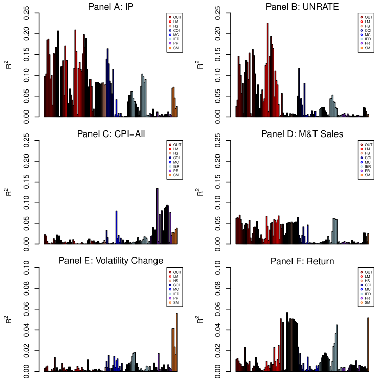
Figure 1: Bar charts of in-sample $R^{2}$s in predicting 1-month ahead industrial production growth (Panel A), unemployment rate (Panel B), consumer price index: all (Panel C), Real Manufacturing and Trade Industries Sales (Panel D), S&P 500 index Volatility Change (Panel E), and the S&P 500 index return (Panel F) by each of the 123 macro variables from the FRED-MD data set of McCracken and Ng (2016), consisting of eight groups including the output and income (OUT), Labor market(LM), Housing (HS), Consumption, orders, and inventories (COI), Money and credit (MC), Interest and exchange rates (IER), Prices (PR), and Stock market (SM). We set $q=2$ in each regression. Macro variables are collected at a monthly frequency and the sample period is 1962:07–2019:12.

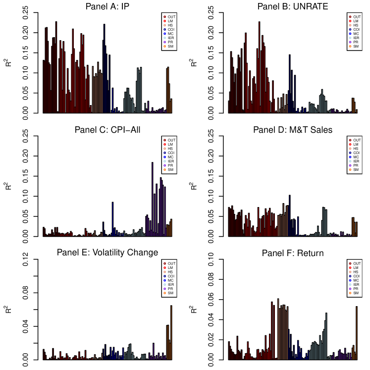
Figure 2: Bar charts of in-sample $R^{2}$s in predicting 1-month ahead industrial production growth (Panel A), unemployment rate (Panel B), consumer price index: all (Panel C), Real Manufacturing and Trade Industries Sales (Panel D), S&P 500 index Volatility Change (Panel E), and the S&P 500 index return (Panel F) by each of the 123 macro variables from the FRED-MD data set of McCracken and Ng (2016), consisting of eight groups including the output and income (OUT), Labor market(LM), Housing (HS), Consumption, orders, and inventories (COI), Money and credit (MC), Interest and exchange rates (IER), Prices (PR), and Stock market (SM). We set $q=3$ in each regression. Macro variables are collected at a monthly frequency and the sample period is 1962:07–2019:12.

Furthermore, we also use AIC to select the linear models used in Step 1 and plot the in-sample $R^{2}$s of predicting the 1-month ahead IP growth, change in UNRATE, change in M&T Sales, change in S&P 500 index volatility, and the S&P 500 index return by each of the 123 macro variables, respectively, in Figure 3, where the maximal order is set to be $q=5$. From Figure 3, we see that the overall pattern of the $R^{2}$’s in each plot is similar to its counterparts in Figures 1 and 2. There are some minor differences between the $R^{2}$ explained by the models with fixed lags and those selected by AIC. For example, the Consumption, orders, and inventories (COI) related variables have more predictive power for IP than those in Figures 1–2, and the Prices (PR) related variables produce slightly higher predictive power for the consumer price index: all (CPI-All). Nevertheless, the findings in Figures 1–2 remain valid in terms of variables that are related to the target variables according to their predictive power.

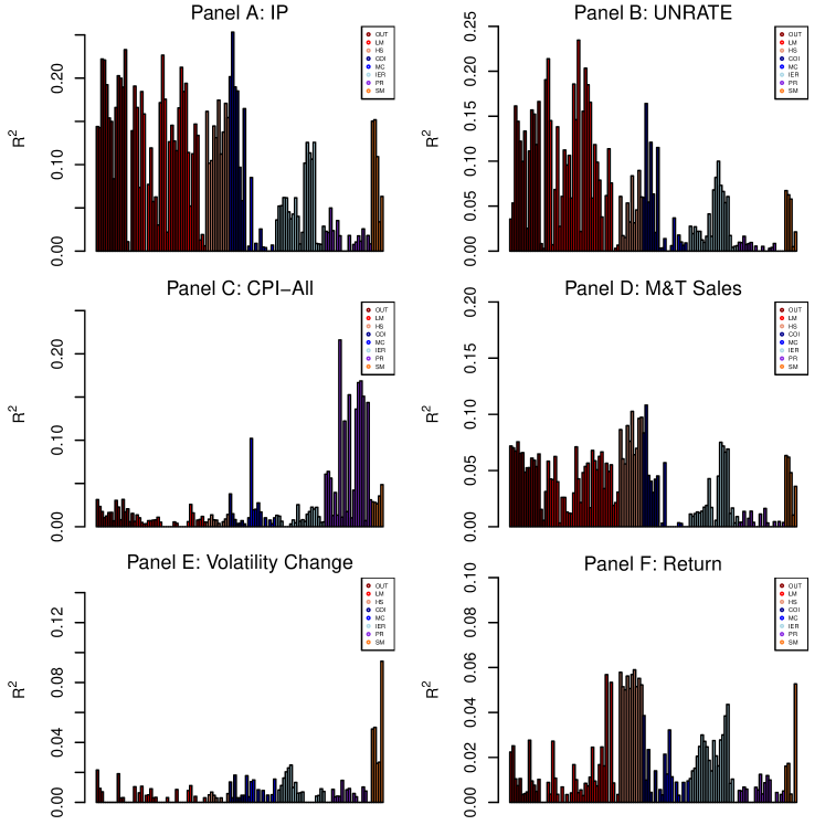
Figure 3: Bar charts of in-sample $R^{2}$s in predicting 1-month ahead industrial production growth (Panel A), unemployment rate (Panel B), consumer price index: all (Panel C), Real Manufacturing and Trade Industries Sales (Panel D), S&P 500 index Volatility Change (Panel E), and the S&P 500 index return (Panel F) by each of the 123 macro variables from the FRED-MD data set of McCracken and Ng (2016), consisting of eight groups including the output and income (OUT), Labor market(LM), Housing (HS), Consumption, orders, and inventories (COI), Money and credit (MC), Interest and exchange rates (IER), Prices (PR), and Stock market (SM). We set $q=5$ in each regression and use AIC to select the model in Step 1. Macro variables are collected at a monthly frequency and the sample period is 1962:07–2019:12.

Next, we consider the in-sample data analysis. First, we standardize each macroeconomic variable and calculate the eigenvalues of the resulting covariance of the 123 variables. That is, we perform eigen-value decomposition of the sample correlation matrix of the predictors. Based on the resulting eigenvalues, the first PCA factor explains about 18% of the total variation. When we apply the proposed sdPCA method to the data, the first sdPCA factor explains 21% to 52% of the total variation depending on the target variable of interest, which is higher than that explained by the first PCA factor. This suggests that the supervised PCA may improve the predictive power of the available predictors.

We plot the loadings of the first to the sixth factors using the traditional PCA method in Figure 4, where, for ease of reading, each loading vector is obtained by multiplying the corresponding eigenvector by 10. From the plot, we see that the first and the second PCA factors are more related to the real economic conditions and they have heavier loads on output and income, labor, and housing variables, followed by the interest and exchange rates. The third PCA factor depends mainly on price-related variables. The fourth factor has heavier loads on the interest rates and stock market conditions. The fifth factor has larger loadings on the interest rates while the sixth factor shows similar loading grouping as those of the first two factors.

For comparison purposes, we also show the first six loadings of the proposed sdPCA in predicting the 1-month ahead IP growth, change of UNRATE, CPI-All, M&T Sales, Volatility Change, and the Return in Figures 5$-$7. From these plots, we see that the loadings are rather different from those in Figure 4. For example, from Figure 5, we see that the first factor in predicting IP growth has loads mainly on OUT, LM, and COI conditions while the effect of the HS seen in the first unsupervised PCA factor has decreased. Similar results are also found for UNRATE where the first sdPCA factor mainly depends on the OUT, LM, and COI. From Figure 6, the first factor in predicting CPI-All is related mainly to the price variables resulting in certain adjustments to those in the first unsupervised PCA factor. The first factor in predicting M&T sales depends relatively heavier on the OUT, LM, and HS than on the others. For the stock market data predictions, we find from Figure 7 that the first sdPCA factor in predicting the S&P volatility change has heavier loads on the SM variables, and this is understandable as they are more directly related. On the other hand, we also find that the first sdPCA factor in predicting the Return is more closely related to the HS conditions, implying that the stock returns and the Housing conditions are related, which, in turn, shows that investors may switch investment between the stock market and the real estate market.

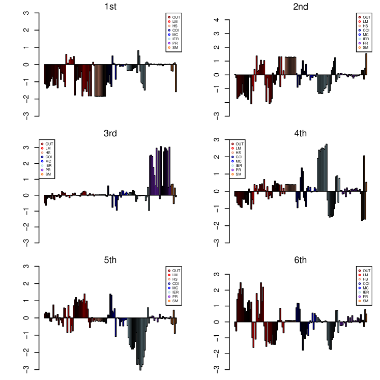
Figure 4: Bar charts of loadings on the 123 macro variables of the first six PCA factors. The macro variables are collected at a monthly frequency from the FRED-MD data set of McCracken and Ng (2016), consisting of eight groups including the output and income (OUT), Labor market(LM), Housing (HS), Consumption, orders, and inventories (COI), Money and credit (MC), Interest and exchange rates (IER), Prices (PR), and Stock market (SM). The sample period is 1962:07–2019:12.

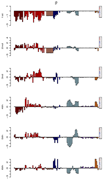
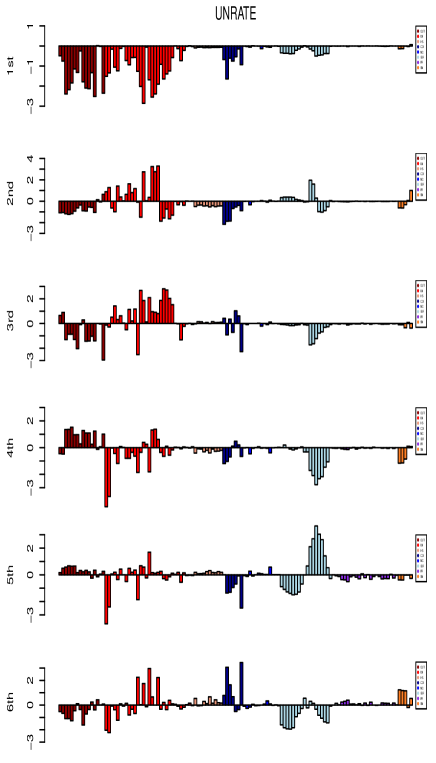
Figure 5: Bar charts of loadings on the 123 macro variables of the first six factors of the proposed sdPCA in predicting the 1-month ahead industrial production growth (OP) and the unemployment rate (UNRATE). The macro variables are collected at a monthly frequency from the FRED-MD data set of McCracken and Ng (2016), consisting of eight groups including the output and income (OUT), Labor market(LM), Housing (HS), Consumption, orders, and inventories (COI), Money and credit (MC), Interest and exchange rates (IER), Prices (PR), and Stock market (SM). The sample period is 1962:07–2019:12.

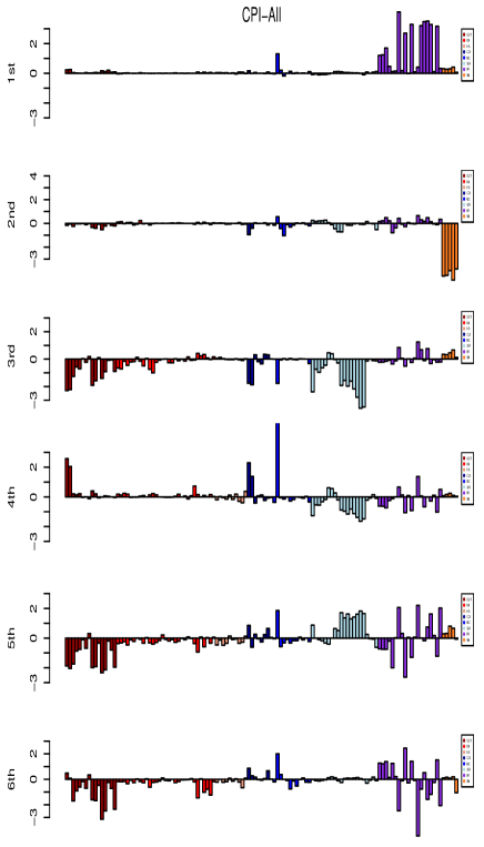
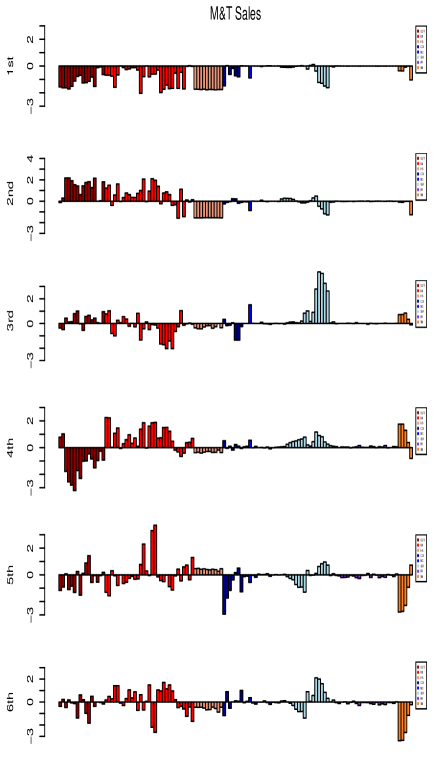
Figure 6: Bar charts of loadings on the 123 macro variables of the first six factors of the proposed sdPCA in predicting the 1-month ahead consumer price index: all (CPI-All) and Real Manufacturing and Trade Industries Sales (M&T Sales). The macro variables are collected at a monthly frequency from the FRED-MD data set of McCracken and Ng (2016), consisting of eight groups including the output and income (OUT), Labor market(LM), Housing (HS), Consumption, orders, and inventories (COI), Money and credit (MC), Interest and exchange rates (IER), Prices (PR), and Stock market (SM). The sample period is 1962:07–2019:12.

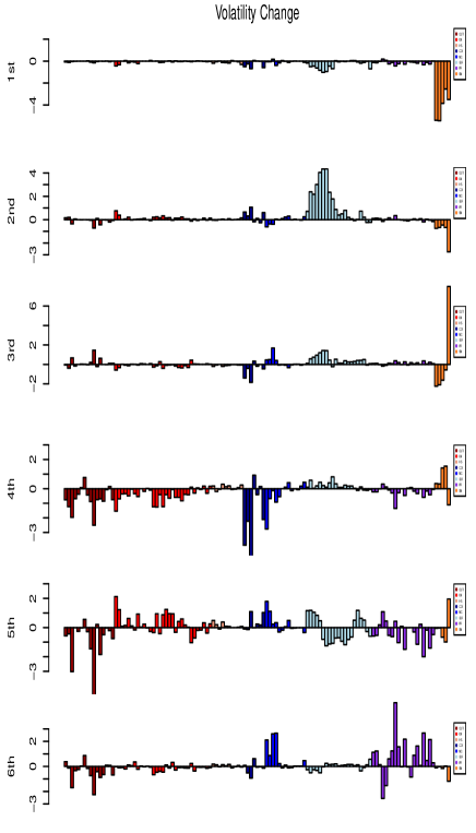
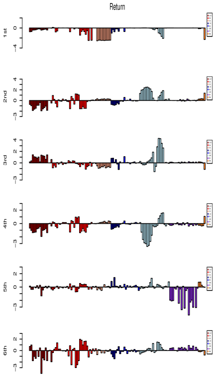
Figure 7: Bar charts of the loadings on the 123 macro variables of the first six sdPCA factors in predicting the 1-month ahead S&P 500 index Volatility Change (Volatility Change), and the S&P 500 index return (Return). The macro variables are collected at a monthly frequency from the FRED-MD data set of McCracken and Ng (2016), consisting of eight groups including the output and income (OUT), Labor market(LM), Housing (HS), Consumption, orders, and inventories (COI), Money and credit (MC), Interest and exchange rates (IER), Prices (PR), and Stock market (SM). The sample period is 1962:07–2019:12.

4.2 Out-of-Sample Forecasting

In this subsection, we assess the performance of the proposed method using out-of-sample forecasting experiments. For each target variable of interest, we split the sample into two subsamples, where the first one consists of the first 80% of the data for modeling and the second subsample of the remaining 20% of the data for out-of-sample prediction. We also adopt the rolling-window scheme as that in the simulation studies, that is, we train the factors and the forecasting coefficients using the first subsample to predict the next target data point. Then we repeat the above procedure after moving the next available observation of predictors and target variable from the second subsample to the first one to obtain the next prediction. This rolling-window scheme is terminated when there is no more observation to compute forecasting error.

Similarly to the experiments in Section 3, we compare the proposed method (sdPCA) with the traditional PCA (denoted by PCA), the sPCA in Huang, Jiang, Li, Tong, and Zhou (2022) (denoted by sPCA), and the diffusion-index forecast in Stock and Watson (2002b) (denoted by SW), where the lagged variables of the PCA factors are also included as predictors in the PCA method, and only the contemporaneous factors are used in the linear forecasting of the SW method. The forecasting performance is measured by the root MSFE defined in (10). We use the autoregressive (AR) model with order 1 or 2 as benchmark methods in the comparison. For the forecasting of IP, UNRATE, CPI-All, and M&T Sales, we consider $h=1,2,3,4,$ and $5$-steps ahead predictions, and we only consider $h=1$ step ahead prediction for the financial data of volatility change and the stock market return, which are of major interest in most financial market predictions.

Tables 5–8 report the results of $h=1,2,3,4$, and $5$-step ahead predictions of the IP, UNRATE, CPI-All, and M&T Sales, respectively. In the comparison, please note that Model (2) implies that the number of factors used in sdPCA is $qs$ if the number of contemporaneous factors used in PCA, sPCA, and the SW is $s$ for an integer $s>0$, where $q$ is the number of lagged variables used in Steps 1 to 3 of the proposed procedure. For the proposed sdPCA, $q=2$ and $q=3$ are employed in the empirical studies, indicating the number of lagged variables used in the forecasting. The number of factors used ranges from 1 to 3 for the methods of PCA, sPCA, and the SW, and therefore, the number of factors used in sdPCA ranges from 1 to 6 when $q=2$ and from 1 to 9 if $q=3$ according to the above discussion. For each $h$, the smallest value is marked in boldface. The Lasso procedure is considered with the corresponding errors given in the parentheses if sdPCA does not beat other methods. We only report the results of the PCA method when $q=2$ because those with $q=3$ do not show any clear improvement in most cases due to the possibility of overfitting. On the other hand, our analysis suggests that the forecasts with more than 3 factors in PCA, sPCA, and the SW do not necessarily improve the prediction accuracy, and therefore, we only compare the results when the number of factors used ranges from 1 to 3 for the methods of PCA, sPCA, and the SW, and the corresponding number of factors used in sdPCA ranges from 1 to 6 when $q=2$ and from 1 to 9 if $q=3$.

From Table 5, we see that the smallest prediction error is achieved by the proposed sdPCA for each $h$, and the prediction using more lagged variables ($q=3$) can improve the forecasting ability ($q=2$) in most cases. Furthermore, the PCA method tends to produce the second smallest errors since it also includes the lagged variables as predictors, which implies that the lagged variables can be used to improve the forecasting performance of IP. In addition, all the methods outperform the benchmark AR methods.

For the predictions of the UNRATE in Table 6, we note that the sdPCA outperforms other competing methods for short-term predictions, such as the cases when $h=1,2$ and $3$, without using the Lasso approach. For $h=4$ and $5$, the errors accumulated by sdPCA are increasing, but the Lasso approach can significantly reduce the forecasting errors and a simple Lasso procedure can produce even smaller errors than all the other methods, implying that the penalized method is an effective way in selecting the factors that have more predictive power. Similar results are also found for the predictions of CPI in Table 7, where the proposed sdPCA as well as the PCA with lagged factors can outperform other methods in short-term forecasting ($h=1$ and $2$), and the forecasting performance for long-term ahead predictions are not more accurate than those by simple AR approaches. In addition, the Lasso approach can also improve the forecasting performance as shown in the case of using sdPCA with $q=3$. Similar findings are also obtained in predicting the M&T sales in Table 8, and we omit the details.

From Tables 5–8, we see that the proposed sdPCA might produce increased errors for $h$ = 4 and 5, especially when the number of factors used increases. There are two possible explanations. First, for stationary time series, such as those considered in our example, the serial dependence decays exponentially so that as $h$ increases the information of the target variable embedded in the predictors decreases. The forecast errors may increase as $h$ increases with uncertainty approaching the unconditional variance of the target variable. Second, increasing the number of factors used also increases the possibility of overfitting, which may lead to inferior prediction. On the other hand, the Lasso procedure can significantly improve the forecasts, which confirms the overfitting issue when more factors are used without variable selection. This highlights the importance of using the Lasso procedure to select the relevant factors if we do not know how many factors to include in linear forecasting.

Finally, the one-step-ahead predictions of the stock return and the volatility change are shown in Table 9. From Table 9, we see that the performance of the sdPCA is comparable with that of SW in forecasting the Stock return, and the sPCA method cannot beat the benchmark methods overall. For the predictions of the volatility change, we find that the proposed sdPCA outperforms all the other competing methods. The results in Table 9 suggest that the proposed sdPCA could be helpful in forecasting financial data.

Table 5: Out-of-sample root mean squared forecast errors in predicting IP. Four comparison methods are used: the proposed method (sdPCA), the one using the factors and their lagged variables extracted by traditional PCA (denoted by PCA), the scaled PCA by Huang, Jiang, Li, Tong, and Zhou (2022) (denoted sPCA), and the original diffusion-index method in Stock and Watson (2002a) using the factors extracted by PCA without lagged variables (denoted by SW). We also use AR(1) and AR(2) models as benchmark methods in out-of-sample forecasting. For the proposed sdPCA, $q=2$ and $q=3$ are considered. For each $h$, the smallest MSFE is marked in boldface.

	sdPCA ($q=2$)							PCA ($q=2$)
$h$	1 ft	2 fts	3 fts	4 fts	5 fts	6 fts		1 ft	2 fts	3 fts
1	0.080	0.078	0.079	0.080	0.079	0.076		0.085	0.078	0.078
2	0.081	0.079	0.080	$$\mathbf{0.075}$$	0.076	0.079		0.086	0.082	0.081
3	0.085	0.082	0.084	0.082	0.083	0.083		0.086	0.084	0.083
4	0.088	$$\mathbf{0.085}$$	0.088	0.086	0.093	0.127		0.086	0.086	0.088
5	0.090	0.087	0.089	0.087	0.089	0.228		0.088	0.088	0.089
	sPCA				SW				AR
	1 ft	2 fts	3 fts		1 ft	2fts	3fts		AR(1)	AR(2)
1	0.083	0.080	0.081		0.085	0.079	0.080		0.085	0.084
2	0.086	0.082	0.084		0.086	0.082	0.082		0.089	0.085
3	0.088	0.084	0.086		0.086	0.084	0.083		0.090	0.085
4	0.089	0.086	0.088		0.086	0.086	0.086		0.091	0.088
5	0.091	0.094	0.091		0.087	0.089	0.089		0.091	0.090
	sdPCA ($q=3$)
	1 ft	2 fts	3 fts	4 fts	5 fts	6 fts	7 fts	8fts	9fts
1	0.078	0.077	0.077	0.074	0.075	$$\mathbf{0.073}$$	0.074	0.074	0.074
2	0.080	0.079	0.079	0.076	0.077	0.077	0.079	0.078	0.078
3	0.084	0.082	0.084	$$\mathbf{0.080}$$	0.082	0.083	0.083	0.081	0.081
4	0.086	$$\mathbf{0.085}$$	0.087	$$\mathbf{0.085}$$	0.089	0.232	0.181	0.182	0.134
5	0.089	0.088	0.090	$$\mathbf{0.086}$$	0.089	0.096	0.110	0.109	0.120

Table 6: Out-of-sample root mean squared forecast errors in predicting UNRATE. Four comparison methods are used: our proposed method (sdPCA), the one using the factors and their lagged variables extracted by PCA (denoted by PCA), the scaled PCA by Huang, Jiang, Li, Tong, and Zhou (2022) (denoted sPCA), and the original diffusion-index model in Stock and Watson (2002a) using the factors extracted by PCA without lagged variables (denoted by SW). We also use AR(1) and AR(2) models as benchmark methods in out-of-sample forecasting. For the proposed sdPCA, $q=2$ and $q=3$ are considered. For each $h$, the smallest MSFE is marked in boldface. The Lasso procedure is applied and the corresponding errors are placed in parentheses if sdPCA does not outperform the other methods.

	sdPCA ($q=2$)							PCA ($q=2$)
$h$	1 ft	2 fts	3 fts	4 fts	5 fts	6 fts		1 ft	2 fts	3 fts
1	1.713	0.694	1.703	1.714	1.682	1.627		1.976	1.773	1.767
2	1.772	1.764	1.795	1.781	1.757	$$\mathbf{1.680}$$		2.004	1.831	1.832
3	1.821	1.897	1.900	1.834	1.867	1.852		2.009	1.850	1.893
4	8.769	3.082	3.657	4.013	4.887	4.783		2.024	1.890	1.939
						(1.914)
5	2.115	4.370	4.730	4.850	4.903	4.774		2.029	1.931	1.951
						($$\mathbf{1.924}$$)
	sPCA				SW				AR
	1 ft	2 fts	3 fts		1 ft	2fts	3fts		AR(1)	AR(2)
1	1.736	1.734	1.707		1.973	1.784	1.791		2.044	1.941
2	1.815	1.817	1.833		1.996	1.859	1.852		2.080	1.960
3	1.859	1.919	1.912		2.006	1.877	1.897		2.090	2.027
4	1.882	1.951	1.956		2.014	1.906	1.937		2.092	2.035
5	2.272	4.782	4.752		2.028	1.939	1.955		2.093	2.069
	sdPCA ($q=3$)
	1 ft	2 fts	3 fts	4 fts	5 fts	6 fts	7 fts	8 fts	9 fts
1	1.696	1.683	1.698	1.674	1.600	$$\mathbf{1.594}$$	1.594	1.595	1.594
2	1.755	1.804	1.808	1.756	1.733	1.696	1.708	1.711	1.704
3	$$\mathbf{1.803}$$	2.380	2.108	2.515	2.579	2.590	2.574	2.572	2.629
4	10.011	2.604	3.936	4.207	4.942	4.986	4.798	4.849	4.868
						($$\mathbf{1.881}$$)
5	8.353	4.835	5.299	5.286	5.082	4.976	4.991	5.032	5.129

Table 7: The out-sample root mean squared forecast errors for CPI-ALL. Four comparison methods are used: our proposed method (sdPCA), the one using the factors and their lagged variables extracted by PCA (denoted by PCA), the scales PCA by Huang, Jiang, Li, Tong, and Zhou (2022) (denoted sPCA), and the original diffusion-index method in Stock and Watson (2002a) using the factors extracted by PCA without lagged variables (denoted by SW). We also use AR(1) and AR(2) models as benchmark methods to do out-of-sample forecasting. For the proposed sdPCA, $q=2$ and $q=3$ are considered. For each $h$, the smallest value is marked in boldface. The Lasso procedure is considered with the corresponding errors given in parentheses if sdPCA does not beat other methods.

	sdPCA ($q=2$)							PCA ($q=2$)
$h$	1 ft	2 fts	3 fts	4 fts	5 fts	6 fts		1 ft	2 fts	3 fts
1	0.034	0.032	0.032	0.032	$$\mathbf{0.031}$$	0.032		0.034	0.034	0.034
2	$$\mathbf{0.032}$$	0.033	0.033	0.033	0.033	0.034		0.034	0.034	$$\mathbf{0.032}$$
3	$$\mathbf{0.034}$$	0.036	0.036	0.036	0.036	0.036		$$\mathbf{0.034}$$	0.034	0.034
4	0.035	0.035	0.035	0.035	0.035	0.035		0.034	0.034	0.034
						(0.034)
5	0.052	0.062	0.064	0.055	0.045	0.044		$$\mathbf{0.034}$$	0.034	0.035
						($$\mathbf{0.034}$$)
	sPCA				SW				AR
	1 ft	2 fts	3 fts		1 ft	2fts	3fts		AR(1)	AR(2)
1	0.035	0.033	0.033		0.034	0.034	0.035		0.035	0.034
2	0.033	0.033	0.033		0.034	0.034	0.033		0.035	0.034
3	$$\mathbf{0.034}$$	0.035	0.036		$$\mathbf{0.034}$$	0.034	0.034		$$\mathbf{0.034}$$	0.035
4	0.034	0.034	0.034		0.034	0.034	0.034		0.034	0.034
5	0.052	0.052	0.049		$$\mathbf{0.034}$$	0.034	0.034		$$\mathbf{0.034}$$	0.034
	sdPCA ($q=3$)
	1 ft	2 fts	3 fts	4 fts	5 fts	6 fts	7 fts	8fts	9 fts
1	0.033	0.032	0.031	0.032	0.032	0.032	0.033	0.032	0.032
2	0.032	0.033	0.033	0.033	0.034	0.034	0.035	0.035	0.035
3	0.035	0.034	0.036	0.036	0.036	0.034	0.038	0.039	0.039
4	0.035	0.034	0.036	0.036	0.036	0.036	0.037	0.037	0.037
						($$\mathbf{0.032}$$)
5	0.060	0.072	0.074	0.058	0.056	0.055	0.052	0.051	0.051

Table 8: The out-sample root mean squared forecast errors for Real Manu. and Trade Industries Sales. Four comparison methods are used: our proposed method (sdPCA), the one using the factors and their lagged variables extracted by PCA (denoted by PCA), the scales PCA by Huang, Jiang, Li, Tong, and Zhou (2022) (denoted sPCA), and the original diffusion-index method in Stock and Watson (2002a) using the factors extracted by PCA without lagged variables (denoted by SW). We also use AR(1) and AR(2) models as benchmark methods to do out-of-sample forecasting. For the proposed sdPCA, $q=2$ and $q=3$ are considered. For each $h$, the smallest value is marked in boldface. The Lasso procedure is considered with the corresponding errors given in parentheses if sdPCA does not beat other methods.

	sdPCA ($q=2$)							PCA ($q=2$)
$h$	1 ft	2 fts	3 fts	4 fts	5 fts	6 fts		1 ft	2 fts	3 fts
1	0.081	$$\mathbf{0.078}$$	0.081	0.082	0.081	0.082		0.081	$$\mathbf{0.078}$$	0.080
2	0.081	$$\mathbf{0.079}$$	0.082	0.080	0.080	0.080		0.081	0.081	0.083
3	0.084	$$\mathbf{0.081}$$	0.085	0.083	0.083	0.084		0.082	0.082	0.083
4	0.086	0.277	0.263	0.291	0.300	0.280		$$\mathbf{0.084}$$	0.084	0.084
						($$\mathbf{0.084}$$)
5	0.087	0.286	0.255	0.289	0.284	0.295		$$\mathbf{0.084}$$	0.085	0.085
	sPCA				SW				AR
	1 ft	2 fts	3 fts		1 ft	2fts	3fts		AR(1)	AR(2)
1	0.084	0.081	0.084		0.082	0.081	0.081		0.090	0.090
2	0.084	0.080	0.083		0.081	0.081	0.082		0.086	0.086
3	0.085	0.083	0.084		0.082	0.083	0.084		0.087	0.087
4	0.087	0.090	0.088		0.084	0.085	0.085		0.087	0.087
5	0.087	0.212	0.235		$$\mathbf{0.084}$$	0.085	0.086		0.087	0.087
	sdPCA ($q=3$)
	1 ft	2 fts	3 fts	4 fts	5 fts	6 fts	7 fts	8 fts	9 fts
1	0.080	0.078	0.080	0.080	0.080	0.081	0.085	0.088	0.086
2	0.081	0.080	0.083	0.080	0.080	0.080	0.083	0.083	0.083
3	0.083	0.250	0.372	0.281	0.268	0.265	0.277	0.257	0.258
4	0.085	0.285	0.286	0.334	0.337	0.316	0.328	0.332	0.334
5	0.086	0.356	0.304	0.322	0.313	0.317	0.309	0.314	0.311
						($$\mathbf{0.084}$$)

Table 9: The out-sample root mean squared forecast errors for S&P 500 index returns and change of S&P 500 index volatility. Four comparison methods are used: our proposed method (sdPCA), the one using the factors and their lagged variables extracted by PCA (denoted by PCA), the scales PCA by Huang, Jiang, Li, Tong, and Zhou (2022) (denoted sPCA), and the original diffusion-index method in Stock and Watson (2002a) using the factors extracted by PCA without lagged variables (denoted by SW). We also use AR(1) and AR(2) models as benchmark methods to do out-of-sample forecasting. For the proposed sdPCA, $q=2$ and $q=3$ are considered. For each $h$, the smallest value is marked in boldface. The Lasso procedure is considered with the corresponding errors are placed in parentheses if sdPCA does not beat other methods.

Stock return with dividends
	sdPCA ($q=2$)							PCA ($q=2$)
$h$	1 ft	2 fts	3 fts	4 fts	5 fts	6 fts		1 ft	2 fts	3 fts
1	0.495	0.505	0.514	0.506	0.534	0.517		0.495	0.503	0.510
	sPCA				SW				AR
	1 ft	2 fts	3 fts		1 ft	2fts	3fts		AR(1)	AR(2)
1	0.498	0.506	0.511		$$\mathbf{0.494}$$	0.504	0.506		0.498	0.499
	sdPCA ($q=3$)
	1 ft	2 fts	3 fts	4 fts	5 fts	6 fts	7 fts	8 fts	9 fts
1	$$\mathbf{0.494}$$	0.506	0.508	0.510	0.518	0.525	0.510	0.515	0.522
Change of Volatility
	sdPCA ($q=2$)							PCA ($q=2$)
$h$	1 ft	2 fts	3 fts	4 fts	5 fts	6 fts		1 ft	2 fts	3 fts
1	$$\mathbf{0.270}$$	0.272	0.270	0.279	0.278	0.271		0.279	0.276	0.278
	sPCA				SW				AR
	1 ft	2 fts	3 fts		1 ft	2fts	3fts		AR(1)	AR(2)
1	0.273	0.271	0.278		0.280	0.280	0.280		0.284	0.286
	sdPCA ($q=3$)
	1 ft	2 fts	3 fts	4 fts	5 fts	6 fts	7 fts	8 fts	9 fts
1	0.270	0.280	0.283	0.277	0.275	0.274	0.274	0.277	0.280

5 Conclusion

This paper introduced a new supervised dynamic PCA method for linear forecasting with many predictors, which is commonly seen in the big-data environment. The new supervised PCA provides an effective way to bridge the gap between predictors and the targeted variables of interest by scaling and combining information of the predictors and their lagged variables, which is in line with dynamic forecasting. Furthermore, we also proposed to use penalized methods, such as the LASSO approach, to select the significant factors that have more predictive power than the others in the linear forecasting equation.

To highlight the prediction power achieved by the proposed method, we showed that our estimators are consistent and outperform theoretically the traditional methods in prediction under some commonly used conditions. We conducted extensive simulations to verify that the proposed method produces satisfactory forecasting results and outperforms most of the existing methods using the traditional PCA. A real data example on predicting U.S. monthly macroeconomic variables using a large number of predictors shows that our method performs better than most of the existing ones in forecasting the U.S. industrial production (IP) growth, change in the unemployment rate (UNRATE), the consumer price index: all (CPI-All), the S&P 500 index volatility change (Volatility Change), and the S&P 500 index return with 123 macro variables from FRED-MD. Finally, the proposed sdPCA together with the Lasso procedure produces even more satisfactory results in many cases. Overall, the proposed procedure provides a comprehensive and effective method for dynamic forecasting when the data dimension is large.

Internet Appendix for
Supervised Dynamic PCA: Linear Dynamic Forecasting with Many Predictors

The first part of the Internet Appendix provides detailed proofs for all the theoretical statements in the main text, and the second part presents descriptions of the real data used in the main article.

Keywords: Dynamic Forecasting, Factor Analysis, Supervised Principal Components, Large-Dimension, LASSO

JEL classification: C22, C23, C38, C53

IA.A Proofs of the Theorems

We need some lemmas first and use $C$ or $c$ to denote a generic constant the value of which may change at different places. The same notations as those of the main article are used throughout.

Let ${\mathbf{u}}_{t}=(u_{1,t},...,u_{N,t})^{\prime}$, ${\mathbf{u}}_{i}=(u_{i,1},...,u_{i,T})^{\prime}$, and ${\mathbf{U}}$ and ${\mathbf{F}}$ be the two matrices consisting ${\mathbf{u}}_{t}^{\prime}$ and ${\mathbf{f}}_{t}^{\prime}$ as their corresponding rows. The following lemma will be used either explicitly or implicitly in the proofs of the theorems of the main article.

Lemma 1.

Let Assumptions 1$-$6 hold. For each $t$, (i) $E\|N^{-\nu/2}\sum_{i}{\mathbf{b}}_{i}u_{i,t}\|^{2}\leq C$, (ii) for each $i$, $\frac{1}{NT}{\mathbf{u}}_{t}^{\prime}{\mathbf{U}}^{\prime}{\mathbf{F}}=O_{p}(\delta_{NT}^{2})$, where $\delta_{NT}=\min\{\sqrt{N},\sqrt{T}\}$, (iii) $E\|T^{-1/2}\sum_{t}{\mathbf{f}}_{t}u_{i,t}||^{2}\leq C$, (iv) $\frac{1}{N^{\nu}T}{\mathbf{u}}_{i}^{\prime}{\mathbf{U}}{\mathbf{B}}=O_{p}(\frac{1}{N^{\nu}})+O_{p}(\frac{1}{\sqrt{TN^{\nu}}})$; (v) ${\mathbf{B}}^{\prime}{\mathbf{U}}^{\prime}{\mathbf{F}}=\sum_{i=1}^{N}\sum_{t=1}^{T}{\mathbf{b}}_{i}{\mathbf{f}}_{t}^{\prime}u_{i,t}=O_{p}(\sqrt{N^{\nu}T})$.

Proof. The results are the same as those in Assumption A3 in Bai and Ng (2023). They can be shown via elementary argument under Assumptions 1-6. We omit the details. $\Box$ Without loss of generality, we assume the data are centered so that the intercepts will be removed from the model. Then the model can be written as

$$\left\{\begin{array}[]{c}{\mathbf{x}}_{t}={\mathbf{B}}{\mathbf{f}}_{t}+{\mathbf{u}}_{t}\\ y_{t+h}={\mathbf{g}}_{t}^{\prime}\boldsymbol{\beta}+\mbox{\boldmath$\varepsilon$}_{t+h},\end{array}\right.$$ (IA.1)

where ${\mathbf{g}}_{t}=({\mathbf{f}}_{t}^{\prime},{\mathbf{f}}_{t-1}^{\prime},...,{\mathbf{f}}_{t-q+1}^{\prime})^{\prime}$ and $\boldsymbol{\beta}=(\boldsymbol{\beta}_{0},\boldsymbol{\beta}_{1},...,\boldsymbol{\beta}_{q-1}^{\prime})^{\prime}$ for $q\geq 1$. Let ${\mathbf{x}}_{i,t}=(x_{i,t},x_{i,t-1},...,x_{i,t-q+1})^{\prime}$, without loss of generality, we assume that

$$\frac{1}{T}\sum_{t=q}^{T-h}{\mathbf{x}}_{i,t}{\mathbf{x}}_{i,t}^{\prime}={\mathbf{I}}_{q}\,\,\text{and}\,\,\frac{1}{T}\sum_{t=q}^{T-h}{\mathbf{g}}_{t}{\mathbf{g}}_{t}^{\prime}={\mathbf{I}}_{rq}.$$ (IA.2)

Letting $\widehat{\boldsymbol{\gamma}}_{i}=(\widehat{\gamma}_{i,0},...,\widehat{\gamma}_{i,q-1})^{\prime}$ and $\boldsymbol{\xi}_{i,t}=(u_{i,t},...,u_{i,t-q+1})^{\prime}$, by least-squares estimation and the identification condition in (IA.2), we have

$$\widehat{\boldsymbol{\gamma}}_{i}= \{({\mathbf{I}}_{q}\otimes{\mathbf{b}}_{i}^{\prime})\boldsymbol{\beta}\}+\left\{({\mathbf{I}}_{q}\otimes{\mathbf{b}}_{i}^{\prime})\frac{1}{T}\sum_{t=q}^{T-h}{\mathbf{g}}_{t}\mbox{\boldmath$\varepsilon$}_{t+h}+\frac{1}{T}\sum_{t=q}^{T-h}\boldsymbol{\xi}_{i,t}{\mathbf{g}}_{t}^{\prime}\boldsymbol{\beta}+\frac{1}{T}\sum_{t=q}^{T-h}\boldsymbol{\xi}_{i,t}\mbox{\boldmath$\varepsilon$}_{t+h}\right\}$$

$$= \boldsymbol{\gamma}_{i}+\boldsymbol{\delta}_{i}.$$ (IA.3)

Roughly speaking, each term in $\boldsymbol{\delta}_{i}$ is of order $O_{p}(1/\sqrt{T})$. Letting

$$z_{i,t}=\widehat{\boldsymbol{\gamma}}_{i}^{\prime}({\mathbf{I}}_{q}\otimes{\mathbf{b}}_{i}^{\prime}){\mathbf{g}}_{t}+\widehat{\boldsymbol{\gamma}}_{i}^{\prime}\boldsymbol{\xi}_{i,t},$$

we have the following lemma.

Lemma 2.

Let ${\mathbf{Z}}_{i}=(z_{i,q},...,z_{i,T-h})^{\prime}$ and $\widetilde{\mathbf{V}}$ be the diagonal matrix consisting of the top $qr$ eigenvalues of $\sum_{i=1}^{N}{\mathbf{Z}}_{i}{\mathbf{Z}}_{i}^{\prime}$ as its diagonal elements. Under Assumptions 1$-$6, if $N^{1-\nu}/T^{2}\rightarrow 0$, with probability tending to one, we have

$$\widetilde{\mathbf{V}}\asymp N^{\nu}T.$$

Proof. Let ${\mathbf{G}}=({\mathbf{g}}_{q},...,{\mathbf{g}}_{T-h})^{\prime}$ and $\boldsymbol{\xi}_{i}=(\boldsymbol{\xi}_{i,q}^{\prime},...,\boldsymbol{\xi}_{i,T-h}^{\prime})^{\prime}$. It follows that

$${\mathbf{Z}}_{i}={\mathbf{G}}(\widehat{\boldsymbol{\gamma}}_{i}\otimes{\mathbf{b}}_{i})+({\mathbf{I}}_{m}\otimes\widehat{\boldsymbol{\gamma}}_{i}^{\prime})\boldsymbol{\xi}_{i},$$

where $m=T-q-h+1$. Then,

$${\mathbf{Z}}_{i}{\mathbf{Z}}_{i}^{\prime}= {\mathbf{G}}(\widehat{\boldsymbol{\gamma}}_{i}\widehat{\boldsymbol{\gamma}}_{i}^{\prime}\otimes{\mathbf{b}}_{i}{\mathbf{b}}_{i}^{\prime}){\mathbf{G}}^{\prime}+{\mathbf{G}}(\widehat{\boldsymbol{\gamma}}_{i}\otimes{\mathbf{b}}_{i})\boldsymbol{\xi}_{i}^{\prime}({\mathbf{I}}_{m}\otimes\widehat{\boldsymbol{\gamma}}_{i})$$

$$+({\mathbf{I}}_{m}\otimes\widehat{\boldsymbol{\gamma}}_{i}^{\prime})\boldsymbol{\xi}_{i}(\widehat{\boldsymbol{\gamma}}_{i}^{\prime}\otimes{\mathbf{b}}_{i}^{\prime}){\mathbf{G}}^{\prime}+({\mathbf{I}}_{m}\otimes\widehat{\boldsymbol{\gamma}}_{i}^{\prime})\boldsymbol{\xi}_{i}\boldsymbol{\xi}_{i}^{\prime}({\mathbf{I}}_{m}\otimes\widehat{\boldsymbol{\gamma}}_{i}).$$ (IA.4)

By definition, if $\widetilde{\mathbf{G}}$ consists of the eigenvectors of $\sum_{i=1}^{N}{\mathbf{Z}}_{i}{\mathbf{Z}}_{i}^{\prime}$ as its columns, we have

$$\widetilde{\mathbf{V}}= \widetilde{\mathbf{G}}^{\prime}\sum_{i=1}^{N}{\mathbf{Z}}_{i}{\mathbf{Z}}_{i}^{\prime}\widetilde{\mathbf{G}}$$

$$= \widetilde{\mathbf{G}}^{\prime}[{\mathbf{G}}\sum_{i=1}^{N}(\widehat{\boldsymbol{\gamma}}_{i}\widehat{\boldsymbol{\gamma}}_{i}^{\prime}\otimes{\mathbf{b}}_{i}{\mathbf{b}}_{i}^{\prime}){\mathbf{G}}^{\prime}]\widetilde{\mathbf{G}}+\widetilde{\mathbf{G}}^{\prime}[{\mathbf{G}}\sum_{i=1}^{N}(\widehat{\boldsymbol{\gamma}}_{i}\otimes{\mathbf{b}}_{i})\boldsymbol{\xi}_{i}^{\prime}({\mathbf{I}}_{m}\otimes\widehat{\boldsymbol{\gamma}}_{i})]\widetilde{\mathbf{G}}$$

$$+\widetilde{\mathbf{G}}^{\prime}[\sum_{i=1}^{N}({\mathbf{I}}_{m}\otimes\widehat{\boldsymbol{\gamma}}_{i}^{\prime})\boldsymbol{\xi}_{i}(\widehat{\boldsymbol{\gamma}}_{i}^{\prime}\otimes{\mathbf{b}}_{i}^{\prime}){\mathbf{G}}^{\prime}]\widetilde{\mathbf{G}}+\widetilde{\mathbf{G}}^{\prime}[\sum_{i=1}^{N}({\mathbf{I}}_{m}\otimes\widehat{\boldsymbol{\gamma}}_{i}^{\prime})\boldsymbol{\xi}_{i}\boldsymbol{\xi}_{i}^{\prime}({\mathbf{I}}_{m}\otimes\widehat{\boldsymbol{\gamma}}_{i})]\widetilde{\mathbf{G}}$$

$$= I_{1}+I_{2}+I_{3}+I_{4}.$$ (IA.5)

Let $\mathcal{I}_{b}$ be the set of indices whose ${\mathbf{b}}_{i}$ is not zero and $\mathcal{I}_{b}^{c}$ be its complement set. Then $|\mathcal{I}_{b}|=N^{\nu}$, $\widehat{\boldsymbol{\gamma}}_{i}=\boldsymbol{\gamma}_{i}+\boldsymbol{\delta}_{i}$ in set $\mathcal{I}_{b}$, and $\widehat{\boldsymbol{\gamma}}_{i}=\boldsymbol{\delta}_{i}$ in set $\mathcal{I}_{b}^{c}$. We first consider $I_{1}$ in (IA.A). Note that $\widehat{\boldsymbol{\gamma}}_{i}=\boldsymbol{\gamma}_{i}+\boldsymbol{\delta}_{i}$, therefore,

$$I_{1}= \widetilde{\mathbf{G}}^{\prime}[{\mathbf{G}}\sum_{i\in\mathcal{I}_{b}}((\boldsymbol{\gamma}_{i}+\boldsymbol{\delta}_{i})(\boldsymbol{\gamma}_{i}+\boldsymbol{\delta}_{i})^{\prime}\otimes{\mathbf{b}}_{i}{\mathbf{b}}_{i}^{\prime}){\mathbf{G}}^{\prime}]\widetilde{\mathbf{G}}+\widetilde{\mathbf{G}}^{\prime}{\mathbf{G}}\sum_{i\in\mathcal{I}_{b}^{c}}(\boldsymbol{\delta}_{i}\boldsymbol{\delta}_{i}^{\prime}\otimes{\mathbf{b}}_{i}{\mathbf{b}}_{i}^{\prime}){\mathbf{G}}^{\prime}\widetilde{\mathbf{G}}$$

$$= \widetilde{\mathbf{G}}^{\prime}{\mathbf{G}}(\sum_{i\in\mathcal{I}_{b}}\boldsymbol{\gamma}_{i}\boldsymbol{\gamma}_{i}^{\prime}\otimes{\mathbf{b}}_{i}{\mathbf{b}}_{i}^{\prime}){\mathbf{G}}^{\prime}\widetilde{\mathbf{G}}+\widetilde{\mathbf{G}}^{\prime}{\mathbf{G}}\sum_{i\in\mathcal{I}_{b}}(\boldsymbol{\gamma}_{i}\boldsymbol{\delta}_{i}^{\prime}\otimes{\mathbf{b}}_{i}{\mathbf{b}}_{i}^{\prime}){\mathbf{G}}^{\prime}\widetilde{\mathbf{G}}+\widetilde{\mathbf{G}}^{\prime}{\mathbf{G}}(\sum_{i\in\mathcal{I}_{b}}\boldsymbol{\delta}_{i}\boldsymbol{\gamma}_{i}^{\prime}\otimes{\mathbf{b}}_{i}{\mathbf{b}}_{i}^{\prime}){\mathbf{G}}^{\prime}\widetilde{\mathbf{G}}$$

$$+\widetilde{\mathbf{G}}^{\prime}{\mathbf{G}}\sum_{i=1}^{N}(\boldsymbol{\delta}_{i}\boldsymbol{\delta}_{i}^{\prime}\otimes{\mathbf{b}}_{i}{\mathbf{b}}_{i}^{\prime}){\mathbf{G}}^{\prime}\widetilde{\mathbf{G}}$$

$$= I_{1,1}+I_{1,2}+I_{1,3}+I_{1,4}.$$ (IA.6)

Note that $\|\widetilde{\mathbf{G}}\|=O_{p}(1)$ and $\|{\mathbf{G}}\|=O_{p}(\sqrt{T})$, by Assumptions 1$-$3, it is not hard to show that

$$\|I_{1,1}\|=O_{P}(N^{\nu}T).$$ (IA.7)

Since $\|\boldsymbol{\delta}_{i}\|=O_{p}(1/\sqrt{T})$, we can similarly show that

$$\|I_{1,2}\|=O_{p}(N^{\nu}T^{1/2}),\|I_{1,3}\|=O_{p}(N^{\nu}T^{1/2}),\,\,\text{and}\,\,\|I_{1,4}\|=O_{p}(N^{\nu}).$$ (IA.8)

It follows from (IA.7)–(IA.8) that

$$\|I_{1}\|=O_{p}(N^{\nu}T+N^{\nu}T^{1/2}+N^{\nu})=O_{p}(N^{\nu}T).$$ (IA.9)

Consider $I_{2}$, which is

$$I_{2}= \widetilde{\mathbf{G}}^{\prime}[{\mathbf{G}}\sum_{i=1}^{N}(\widetilde{\boldsymbol{\gamma}}_{i}\otimes{\mathbf{b}}_{i})\boldsymbol{\xi}_{i}^{\prime}({\mathbf{I}}_{m}\otimes\widetilde{\boldsymbol{\gamma}}_{i})]\widetilde{\mathbf{G}}$$

$$= \widetilde{\mathbf{G}}^{\prime}[{\mathbf{G}}\sum_{i\in\mathcal{I}_{b}}((\widetilde{\boldsymbol{\gamma}}_{i}+\boldsymbol{\delta}_{i})\otimes{\mathbf{b}}_{i})\boldsymbol{\xi}_{i}^{\prime}({\mathbf{I}}_{m}\otimes(\boldsymbol{\gamma}_{i}+\boldsymbol{\delta}_{i}))]\widetilde{\mathbf{G}}+\widetilde{\mathbf{G}}^{\prime}{\mathbf{G}}\sum_{i\in\mathcal{I}_{b}^{c}}(\boldsymbol{\delta}_{i}\otimes{\mathbf{b}}_{i})\boldsymbol{\xi}_{i}^{\prime}({\mathbf{I}}_{m}\otimes\boldsymbol{\delta}_{i})\widetilde{\mathbf{G}}$$

$$= \widetilde{\mathbf{G}}^{\prime}{\mathbf{G}}\sum_{i\in\mathcal{I}_{b}}(\boldsymbol{\gamma}_{i}\otimes{\mathbf{b}}_{i})\boldsymbol{\xi}_{i}^{\prime}({\mathbf{I}}_{m}\otimes\boldsymbol{\gamma}_{i})\widetilde{\mathbf{G}}+\widetilde{\mathbf{G}}^{\prime}{\mathbf{G}}\sum_{i\in\mathcal{I}_{b}}(\boldsymbol{\gamma}_{i}\otimes{\mathbf{b}}_{i})\boldsymbol{\xi}_{i}^{\prime}({\mathbf{I}}_{m}\otimes\boldsymbol{\delta}_{i})\widetilde{\mathbf{G}}$$

$$+\widetilde{\mathbf{G}}^{\prime}{\mathbf{G}}\sum_{i\in\mathcal{I}_{b}}(\boldsymbol{\delta}_{i}\otimes{\mathbf{b}}_{i})\boldsymbol{\xi}_{i}^{\prime}({\mathbf{I}}_{m}\otimes\boldsymbol{\gamma}_{i})\widetilde{\mathbf{G}}+\widetilde{\mathbf{G}}^{\prime}{\mathbf{G}}\sum_{i=1}^{N}(\boldsymbol{\delta}_{i}\otimes{\mathbf{b}}_{i})\boldsymbol{\xi}_{i}^{\prime}({\mathbf{I}}_{m}\otimes\boldsymbol{\delta}_{i})\widetilde{\mathbf{G}}$$

$$= I_{2,1}+I_{2,2}+I_{2,3}+I_{2,4}.$$ (IA.10)

Note that

$$\sum_{i\in\mathcal{I}_{b}}(\boldsymbol{\gamma}_{i}\otimes{\mathbf{b}}_{i})\boldsymbol{\xi}_{i}^{\prime}({\mathbf{I}}_{m}\otimes\boldsymbol{\gamma}_{i})\widetilde{\mathbf{G}}= \sum_{i\in\mathcal{I}_{b}}(\boldsymbol{\gamma}_{i}\otimes{\mathbf{b}}_{i})\sum_{t=q}^{T-h}\boldsymbol{\xi}_{i,t}^{\prime}\boldsymbol{\gamma}_{i}\widetilde{\mathbf{g}}_{t}^{\prime}$$

$$= \sum_{t=q}^{T-h}\sum_{i\in\mathcal{I}_{b}}(\boldsymbol{\gamma}_{i}\otimes{\mathbf{b}}_{i})\boldsymbol{\gamma}_{i}^{\prime}\boldsymbol{\xi}_{i,t}\widetilde{\mathbf{g}}_{t}^{\prime}$$

$$\leq \left(\sum_{t=q}^{T-h}|\sum_{i\in\mathcal{I}_{b}}(\boldsymbol{\gamma}_{i}\otimes{\mathbf{b}}_{i})\boldsymbol{\gamma}_{i}^{\prime}\boldsymbol{\xi}_{i,t}|^{2}\right)^{1/2}\left(\sum_{t=q}^{T-h}\|\widetilde{\mathbf{g}}_{t}\|^{2}\right)^{1/2}$$

$$= O_{p}\{(T(N^{\nu/2})^{2})^{1/2}\}O_{p}(1)$$

$$= O_{p}(N^{\nu/2}T^{1/2}),$$ (IA.11)

which implies that

$$\|I_{2,1}\|=\|\widetilde{\mathbf{G}}^{\prime}{\mathbf{G}}\|O_{p}(N^{\nu/2}T^{1/2})=O_{p}(N^{\nu/2}T).$$ (IA.12)

Recall that

$$\boldsymbol{\delta}_{i}= \left\{\frac{1}{T}\sum_{t=q}^{T-h}\boldsymbol{\xi}_{i,t}{\mathbf{g}}_{t}^{\prime}\boldsymbol{\beta}+\frac{1}{T}\sum_{t=q}^{T-h}\boldsymbol{\xi}_{i,t}\mbox{\boldmath$\varepsilon$}_{t+h}\right\}+\left\{({\mathbf{I}}_{q}\otimes{\mathbf{b}}_{i}^{\prime})\frac{1}{T}\sum_{t=q}^{T-h}{\mathbf{g}}_{t}\mbox{\boldmath$\varepsilon$}_{t+h}\right\}$$

$$= \boldsymbol{\delta}_{i,1}+\boldsymbol{\delta}_{i,2}.$$ (IA.13)

We now consider $I_{2,2}$. First,

$$\sum_{i\in\mathcal{I}_{b}}(\boldsymbol{\gamma}_{i}\otimes{\mathbf{b}}_{i})\boldsymbol{\xi}_{i}^{\prime}({\mathbf{I}}_{m}\otimes\boldsymbol{\delta}_{i,2})\widetilde{\mathbf{G}}=O_{p}(N^{\nu/2}),$$

and

$$\sum_{i\in\mathcal{I}_{b}}(\boldsymbol{\gamma}_{i}\otimes{\mathbf{b}}_{i})\boldsymbol{\xi}_{i}^{\prime}({\mathbf{I}}_{m}\otimes\boldsymbol{\delta}_{i,1})\widetilde{\mathbf{G}}= \sum_{i\in\mathcal{I}_{b}}(\boldsymbol{\gamma}_{i}\otimes{\mathbf{b}}_{i})\boldsymbol{\delta}_{i,1}^{\prime}\sum_{t=q}^{T-h}\boldsymbol{\xi}_{i,t}\widetilde{\mathbf{g}}_{t}^{\prime}$$

$$= \frac{1}{T}\sum_{t=q}^{T-h}\sum_{s=q}^{T-h}w_{t}[\sum_{i\in\mathcal{I}_{b}}(\boldsymbol{\gamma}_{i}\otimes{\mathbf{b}}_{i})\boldsymbol{\xi}_{i,s}^{\prime}\boldsymbol{\xi}_{it}]\widetilde{\mathbf{g}}_{s}^{\prime}$$

$$= \frac{1}{T}\sum_{t=q}^{T-h}\sum_{s=q}^{T-h}w_{t}[\sum_{i\in\mathcal{I}_{b}}(\boldsymbol{\gamma}_{i}\otimes{\mathbf{b}}_{i})(\boldsymbol{\xi}_{i,s}^{\prime}\boldsymbol{\xi}_{it}-E\boldsymbol{\xi}_{i,s}^{\prime}\boldsymbol{\xi}_{it})]\widetilde{\mathbf{g}}_{s}^{\prime}$$

$$+\frac{1}{T}\sum_{t=q}^{T-h}\sum_{s=q}^{T-h}w_{t}[\sum_{i\in\mathcal{I}_{b}}(\boldsymbol{\gamma}_{i}\otimes{\mathbf{b}}_{i})E\boldsymbol{\xi}_{i,s}^{\prime}\boldsymbol{\xi}_{it}]\widetilde{\mathbf{g}}_{s}^{\prime}$$

$$= I_{2,2,1}+I_{2,2,2}.$$ (IA.14)

By the Schwarz inequality, we have

$$I_{2,2,1}\leq \frac{1}{T}\left\{\sum_{s=q}^{T-h}[\sum_{t=q}^{T-h}w_{t}\sum_{i\in\mathcal{I}_{b}}(\boldsymbol{\gamma}_{i}\otimes{\mathbf{b}}_{i})(\boldsymbol{\xi}_{i,s}^{\prime}\boldsymbol{\xi}_{it}-E\boldsymbol{\xi}_{i,s}^{\prime}\boldsymbol{\xi}_{it}))]^{2}\right\}^{1/2}\left[\sum_{s=q}^{T-h}\|\widetilde{\mathbf{g}}_{s}\|^{2}\right]^{1/2}$$

$$\leq \frac{1}{T}O_{p}(T(N^{\nu/2}T^{1/2})^{2})^{1/2}O_{p}(1)=O_{p}(N^{\nu/2}),$$ (IA.15)

and

$$I_{2,2,2}= \frac{1}{T}\left(\sum_{s=q}^{T-h}\|\widetilde{\mathbf{g}}_{s}\|^{2}\right)^{1/2}\left(\sum_{s=q}^{T-h}|\sum_{t=q}^{T-h}w_{t}[\sum_{i\in\mathcal{I}_{b}}E\boldsymbol{\xi}_{i,s}^{\prime}\boldsymbol{\xi}_{i,t}]|^{2}\right)^{1/2}$$

$$\leq O_{p}(1/T)O_{p}((T(N^{\nu})^{2})^{1/2})=O_{p}(N^{\nu}T^{-1/2}).$$ (IA.16)

where $w_{t}={\mathbf{g}}_{t}^{\prime}\boldsymbol{\beta}+\mbox{\boldmath$\varepsilon$}_{t+h}$. Since $\|{\mathbf{G}}\|=O_{p}(T^{1/2})$, it follows that

$$I_{2,2}=O_{p}(N^{\nu/2}T^{1/2}+N^{\nu}).$$

Similarly, we can show that

$$I_{2,3}=O_{p}(N^{\nu/2}T^{1/2}+N^{\nu}).$$

Consider the last term in $I_{2,2}$,

$$I_{2,4}= \widetilde{\mathbf{G}}[{\mathbf{G}}\sum_{i=1}^{N}(\boldsymbol{\delta}_{i,1}\otimes{\mathbf{b}}_{i})\boldsymbol{\xi}_{i}^{\prime}({\mathbf{I}}_{m}\otimes\boldsymbol{\delta}_{i,1})]\widetilde{\mathbf{G}}+\widetilde{\mathbf{G}}[{\mathbf{G}}\sum_{i=1}^{N}(\boldsymbol{\delta}_{i,1}\otimes{\mathbf{b}}_{i})\boldsymbol{\xi}_{i}^{\prime}({\mathbf{I}}_{m}\otimes\boldsymbol{\delta}_{i,2})]\widetilde{\mathbf{G}}$$

$$+\widetilde{\mathbf{G}}[{\mathbf{G}}\sum_{i=1}^{N}(\boldsymbol{\delta}_{i,2}\otimes{\mathbf{b}}_{i})\boldsymbol{\xi}_{i}^{\prime}({\mathbf{I}}_{m}\otimes\boldsymbol{\delta}_{i,1})]\widetilde{\mathbf{G}}+\widetilde{\mathbf{G}}[{\mathbf{G}}\sum_{i=1}^{N}(\boldsymbol{\delta}_{i,2}\otimes{\mathbf{b}}_{i})\boldsymbol{\xi}_{i}^{\prime}({\mathbf{I}}_{m}\otimes\boldsymbol{\delta}_{i,2})]\widetilde{\mathbf{G}}$$

$$= I_{2,4,1}+I_{2,4,2}+I_{2,4,3}+I_{2,4,4}.$$ (IA.17)

We only need to bound the first term as $\boldsymbol{\delta}_{i,1}$ is correlated with $\boldsymbol{\xi}_{i}$ but $\boldsymbol{\delta}_{i,2}$ is not. Since $\|{\mathbf{G}}\|=O_{p}(\sqrt{T})$, $\|\widetilde{\mathbf{G}}\|=O_{p}(1)$, $\|\boldsymbol{\delta}_{i,1}\|=O_{p}(1/\sqrt{T})$, and $\|\boldsymbol{\xi}_{i}\|=O_{p}(\sqrt{T})$, we have

$$I_{2,4,1}= O_{p}(T^{1/2}T^{-1}T^{1/2}N^{\nu})=O_{p}(N^{\nu}).$$ (IA.18)

It follows that

$$\|I_{2,4}\|=O_{p}(N^{\nu}),$$

and, therefore,

$$\|I_{2}\|=O_{p}(N^{\nu/2}T+N^{\nu/2}T^{1/2}+N^{\nu}+N^{\nu})=O_{p}(N^{\nu/2}T+N^{\nu}).$$ (IA.19)

Similarly, we can show that

$$\|I_{3}\|=O_{p}(N^{\nu/2}T+N^{\nu}).$$ (IA.20)

Now turn to $I_{4}$. Noting that $\widehat{\boldsymbol{\gamma}}_{i}=\boldsymbol{\gamma}_{i}+\boldsymbol{\delta}_{i}$ for $i\in\mathcal{I}_{b}$ and $\widehat{\boldsymbol{\gamma}}_{i}=\boldsymbol{\delta}_{i}$ for $i\in\mathcal{I}_{b}^{c}$, we have the following decomposition,

$$I_{4}= \widetilde{\mathbf{G}}^{\prime}[\sum_{i\in\mathcal{I}_{b}}({\mathbf{I}}_{m}\otimes\boldsymbol{\gamma}_{i}^{\prime})\boldsymbol{\xi}_{i}\boldsymbol{\xi}_{i}^{\prime}({\mathbf{I}}_{m}\otimes\boldsymbol{\gamma}_{i})]\widetilde{\mathbf{G}}+\widetilde{\mathbf{G}}^{\prime}[\sum_{i\in\mathcal{I}_{b}}({\mathbf{I}}_{m}\otimes\boldsymbol{\gamma}_{i}^{\prime})\boldsymbol{\xi}_{i}\boldsymbol{\xi}_{i}^{\prime}({\mathbf{I}}_{m}\otimes\boldsymbol{\delta}_{i})]\widetilde{\mathbf{G}}$$

$$+\widetilde{\mathbf{G}}^{\prime}[\sum_{i\in\mathcal{I}_{b}}({\mathbf{I}}_{m}\otimes\boldsymbol{\delta}_{i}^{\prime})\boldsymbol{\xi}_{i}\boldsymbol{\xi}_{i}^{\prime}({\mathbf{I}}_{m}\otimes\boldsymbol{\gamma}_{i})]\widetilde{\mathbf{G}}+\widetilde{\mathbf{G}}^{\prime}[\sum_{i\in\mathcal{I}_{b}}({\mathbf{I}}_{m}\otimes\boldsymbol{\delta}_{i}^{\prime})\boldsymbol{\xi}_{i}\boldsymbol{\xi}_{i}^{\prime}({\mathbf{I}}_{m}\otimes\boldsymbol{\delta}_{i})]\widetilde{\mathbf{G}}$$

$$= I_{4,1}+I_{4,2}+I_{4,3}+I_{4,4}.$$ (IA.21)

We consider the four terms in (IA.A) one by one. First,

$$I_{4,1}= \widetilde{\mathbf{G}}^{\prime}[\sum_{i\in\mathcal{I}_{b}}({\mathbf{I}}_{m}\otimes\boldsymbol{\gamma}_{i}^{\prime})(\boldsymbol{\xi}_{i}\boldsymbol{\xi}_{i}^{\prime}-E\boldsymbol{\xi}_{i}\boldsymbol{\xi}_{i}^{\prime})({\mathbf{I}}_{m}\otimes\boldsymbol{\gamma}_{i})]\widetilde{\mathbf{G}}+\widetilde{\mathbf{G}}^{\prime}[\sum_{i\in\mathcal{I}_{b}}({\mathbf{I}}_{m}\otimes\boldsymbol{\gamma}_{i}^{\prime})(E\boldsymbol{\xi}_{i}\boldsymbol{\xi}_{i}^{\prime})({\mathbf{I}}_{m}\otimes\boldsymbol{\gamma}_{i})]\widetilde{\mathbf{G}}$$

$$= I_{4,1,1}+I_{4,1,2}.$$ (IA.22)

By a similar argument as that in (IA.A)-(IA.A), we have

$$I_{4,1,1}= \sum_{t=q}^{T-h}\sum_{s=q}^{T-h}\widetilde{\mathbf{g}}_{s}\sum_{i\in\mathcal{I}_{b}}\sum_{i\in\mathcal{I}_{b}}\boldsymbol{\gamma}_{i}^{\prime}(\boldsymbol{\xi}_{i,s}\boldsymbol{\xi}_{it}^{\prime}-E\boldsymbol{\xi}_{i,s}\boldsymbol{\xi}_{i,t})\boldsymbol{\gamma}_{i}\widetilde{\mathbf{g}}_{t}^{\prime}$$

$$\leq \left(\sum_{t=q}^{T-h}\|\widetilde{\mathbf{g}}_{t}\|\right)^{1/2}\left(\sum_{t=q}^{T-h}\|\sum_{s=q}^{T-h}\widetilde{\mathbf{g}}_{s}\sum_{i\in\mathcal{I}_{b}}\boldsymbol{\gamma}_{i}^{\prime}(\boldsymbol{\xi}_{i,s}\boldsymbol{\xi}_{i,t}-E\boldsymbol{\xi}_{i,s}\boldsymbol{\xi}_{i,t})\boldsymbol{\gamma}_{i}\|^{2}\right)^{1/2}$$

$$\leq \left(\sum_{t=q}^{T-h}\|\widetilde{\mathbf{g}}_{t}\|\right)\left(\sum_{t=q}^{T-h}\sum_{s=q}^{T-h}(\sum_{i\in\mathcal{I}_{b}}\boldsymbol{\gamma}_{i}^{\prime}(\boldsymbol{\xi}_{i,s}\boldsymbol{\xi}_{i,t}-E\boldsymbol{\xi}_{i,s}\boldsymbol{\xi}_{i,t})\boldsymbol{\gamma}_{i})^{2}\right)^{1/2}$$

$$= O_{p}(1)O_{p}(T^{2}N^{\nu})^{1/2}=O_{P}(N^{\nu/2}T),$$ (IA.23)

and

$$I_{4,1,2}=O_{p}(N^{\nu}).$$

Therefore,

$$I_{4,1}=O_{p}(N^{\nu}+N^{\nu/2}T).$$ (IA.24)

Next,

$$I_{4,2}= \widetilde{\mathbf{G}}[\sum_{i\in\mathcal{I}_{b}}({\mathbf{I}}_{m}\otimes\boldsymbol{\gamma}_{i}^{\prime})\boldsymbol{\xi}_{i}\boldsymbol{\xi}_{i}^{\prime}({\mathbf{I}}_{m}\otimes\boldsymbol{\delta}_{i,1})]\widetilde{\mathbf{G}}+\widetilde{\mathbf{G}}[\sum_{i\in\mathcal{I}_{b}}({\mathbf{I}}_{m}\otimes\boldsymbol{\gamma}_{i}^{\prime})\boldsymbol{\xi}_{i}\boldsymbol{\xi}_{i}^{\prime}({\mathbf{I}}_{m}\otimes\boldsymbol{\delta}_{i,2})]\widetilde{\mathbf{G}}$$

$$= I_{4,2,1}+O_{p}(N^{\nu}T^{-1/2}+N^{\nu/2}T^{1/2}),$$ (IA.25)

where the second rate follows from a similar argument for (IA.24) and the fact that $\boldsymbol{\delta}_{i,2}$ is uncorrelated with $\boldsymbol{\xi}_{i}$. For the first term, we have

$$I_{4,2,1}= \frac{1}{T}\sum_{t=q}^{T-h}\sum_{i\in\mathcal{I}_{b}}\sum_{s=q}^{T-h}\widetilde{\mathbf{g}}_{t}\boldsymbol{\gamma}_{i}^{\prime}\boldsymbol{\xi}_{i,t}\boldsymbol{\xi}_{i,s}^{\prime}\boldsymbol{\delta}_{i,1}\widetilde{\mathbf{g}}_{s}^{\prime}$$

$$= \frac{1}{T}\sum_{t=q}^{T-h}\sum_{s=q}^{T-h}\sum_{l=q}^{T-h}\sum_{i\in\mathcal{I}_{b}}\widetilde{\mathbf{g}}_{t}\boldsymbol{\gamma}_{i}^{\prime}\boldsymbol{\xi}_{i,t}\boldsymbol{\xi}_{i,s}^{\prime}\boldsymbol{\xi}_{i,l}w_{l}\widetilde{\mathbf{g}}_{s}^{\prime}$$

$$\leq \frac{1}{T}\left(\sum_{t=q}^{T-h}\|\widetilde{\mathbf{g}}_{t}\|^{2}\right)\left(\sum_{t=q}^{T-h}\sum_{s=q}^{T-h}(\sum_{l=q}^{T-h}\sum_{i\in\mathcal{I}_{b}}\boldsymbol{\gamma}_{i}^{\prime}\boldsymbol{\xi}_{i,t}\boldsymbol{\xi}_{i,s}^{\prime}\boldsymbol{\xi}_{i,l}w_{l})^{2}\right)^{1/2}$$

$$\leq O_{p}(T^{-1})\left[\sum_{t=q}^{T-h}\sum_{s=q}^{T-h}(\sum_{l=q}^{T-h}w_{l}\sum_{i\in\mathcal{I}_{b}}\boldsymbol{\gamma}_{i}^{\prime}(\boldsymbol{\xi}_{i,t}\boldsymbol{\xi}_{i,s}^{\prime}\boldsymbol{\xi}_{i,l}-E\boldsymbol{\xi}_{i,t}\boldsymbol{\xi}_{i,s}\boldsymbol{\xi}_{i,l}))^{2}\right]^{1/2}$$

$$+O_{p}(T^{-1})\left[\sum_{t=q}^{T-h}\sum_{s=q}^{T-h}(\sum_{l=q}^{T-h}w_{l}\sum_{i\in\mathcal{I}_{b}}\boldsymbol{\gamma}_{i}^{\prime}(E\boldsymbol{\xi}_{i,t}\boldsymbol{\xi}_{i,s}\boldsymbol{\xi}_{i,l}))^{2}\right]^{1/2}$$

$$\leq O_{p}(T^{-1})O_{p}(T^{2}(T^{1/2}N^{\nu/2})^{2})^{1/2}+N^{\nu}T^{-1/2}=O_{p}(N^{\nu/2}T^{1/2}+N^{\nu}T^{-1/2}),$$ (IA.26)

and

$$I_{4,3}=O_{p}(N^{\nu/2}T^{1/2}+N^{\nu}T^{-1/2}).$$

For $I_{4,4}$, we first note that

$$\|I_{4,4}\|\leq 2\|\widetilde{\mathbf{G}}^{\prime}[\sum_{i\in\mathcal{I}_{b}}({\mathbf{I}}_{m}\otimes\boldsymbol{\delta}_{i,1}^{\prime})\boldsymbol{\xi}_{i}\boldsymbol{\xi}_{i}^{\prime}({\mathbf{I}}_{m}\otimes\boldsymbol{\delta}_{i,1})]\widetilde{\mathbf{G}}\|+2\|\widetilde{\mathbf{G}}^{\prime}[\sum_{i\in\mathcal{I}_{b}}({\mathbf{I}}_{m}\otimes\boldsymbol{\delta}_{i,2}^{\prime})\boldsymbol{\xi}_{i}\boldsymbol{\xi}_{i}^{\prime}({\mathbf{I}}_{m}\otimes\boldsymbol{\delta}_{i,2})]\widetilde{\mathbf{G}}\|$$

$$= 2\|I_{4,4,1}\|+2\|I_{4,4,2}\|.$$ (IA.27)

Recall that

$$\boldsymbol{\delta}_{i,1}=\frac{1}{T}\sum_{l=q}^{T-h}\boldsymbol{\xi}_{i,l}w_{l}\,\,\text{and}\,\,\boldsymbol{\delta}_{i,2}=({\mathbf{I}}_{q}\otimes{\mathbf{b}}_{i})^{\prime}\frac{1}{T}\sum_{t=q}^{T-h}{\mathbf{g}}_{t}\mbox{\boldmath$\varepsilon$}_{t+h},$$

then,

$$I_{4,4,1}= \frac{1}{T^{2}}\sum_{t=q}^{T-h}\sum_{s=q}^{t-h}\sum_{l=q}^{T-h}\sum_{k=q}^{T-h}\sum_{i=1}^{N}\widetilde{\mathbf{g}}_{t}w_{t}w_{k}\boldsymbol{\xi}_{i,l}^{\prime}\boldsymbol{\xi}_{i,t}\boldsymbol{\xi}_{i,s}^{\prime}\boldsymbol{\xi}_{i,k}\widetilde{\mathbf{g}}_{s}^{\prime}$$

$$\leq \frac{1}{T^{2}}\sum_{t=q}^{T-h}\sum_{s=q}^{t-h}\sum_{l=q}^{T-h}\sum_{k=q}^{T-h}\sum_{i=1}^{N}\widetilde{\mathbf{g}}_{t}w_{t}w_{k}(\boldsymbol{\xi}_{i,l}^{\prime}\boldsymbol{\xi}_{i,t}\boldsymbol{\xi}_{i,s}^{\prime}\boldsymbol{\xi}_{i,k}-E\boldsymbol{\xi}_{i,l}^{\prime}\boldsymbol{\xi}_{i,t}\boldsymbol{\xi}_{i,s}^{\prime}\boldsymbol{\xi}_{i,k})\widetilde{\mathbf{g}}_{s}^{\prime}$$

$$+\frac{1}{T^{2}}\sum_{t=q}^{T-h}\sum_{s=q}^{t-h}\sum_{l=q}^{T-h}\sum_{k=q}^{T-h}\sum_{i=1}^{N}\widetilde{\mathbf{g}}_{t}w_{t}w_{k}(E\boldsymbol{\xi}_{i,l}^{\prime}\boldsymbol{\xi}_{i,t}\boldsymbol{\xi}_{i,s}^{\prime}\boldsymbol{\xi}_{i,k})\widetilde{\mathbf{g}}_{s}^{\prime}$$

$$= J_{4,1}+J_{4,2}.$$ (IA.28)

$$J_{4,1}\leq \frac{1}{T^{2}}(\sum_{t=q}^{T-h}\|\widetilde{\mathbf{g}}_{t}\|)\left[\sum_{t=q}^{T-h}\sum_{s=q}^{T-h}(\sum_{l=q}^{T-h}\sum_{k=q}^{T-h}\sum_{i=1}^{N}w_{t}w_{k}(\boldsymbol{\xi}_{i,l}^{\prime}\boldsymbol{\xi}_{i,t}\boldsymbol{\xi}_{i,s}^{\prime}\boldsymbol{\xi}_{i,k}-E\boldsymbol{\xi}_{i,l}^{\prime}\boldsymbol{\xi}_{i,t}\boldsymbol{\xi}_{i,s}^{\prime}\boldsymbol{\xi}_{i,k}))^{2}\right]^{1/2}$$

$$\leq \frac{1}{T^{2}}O_{p}(T^{2}(T^{2}N))^{1/2}=O_{p}(N^{1/2}).$$ (IA.29)

$$J_{4,2}\leq\frac{1}{T^{2}}(\sum_{t=q}^{T-h}\sum_{s=q}^{T-h}(\sum_{i=1}^{N}w_{t}^{2}E\boldsymbol{\xi}_{i,t}^{\prime}\boldsymbol{\xi}_{i,t}\boldsymbol{\xi}_{i,s}^{\prime}\boldsymbol{\xi}_{i,s})^{2})^{1/2}=O_{p}(\frac{1}{T^{2}}(T^{2}N^{2})^{1/2})=O_{p}(N/T).$$

It follows that

$$I_{4,4,1}=O_{p}(N^{1/2}+\frac{N}{T}).$$

$$I_{4,4,2}= \sum_{t=q}^{T-h}\sum_{s=q}^{T-h}\widetilde{\mathbf{g}}_{t}\sum_{i=1}^{N}\boldsymbol{\delta}_{i,2}^{\prime}\boldsymbol{\xi}_{i,t}\boldsymbol{\xi}_{i,s}^{\prime}\boldsymbol{\delta}_{i,2}\widetilde{\mathbf{g}}_{s}^{\prime}$$

$$\leq (\sum_{t=q}^{T-h}\|\widetilde{\mathbf{g}}_{t}\|^{2})\left(\sum_{t=q}^{T-h}(\sum_{s=q}^{T-h}\sum_{i=1}^{N}\boldsymbol{\delta}_{i,2}^{\prime}\boldsymbol{\xi}_{i,t}\boldsymbol{\xi}_{i,s}^{\prime}\boldsymbol{\delta}_{i,2})^{2}\right)^{1/2}$$

$$\leq C\left(\sum_{t=q}^{T-h}\sum_{s=q}^{T-h}(\sum_{i=1}^{N}\boldsymbol{\delta}_{i,2}^{\prime}(\boldsymbol{\xi}_{i,t}\boldsymbol{\xi}_{i,s}^{\prime}-E\boldsymbol{\xi}_{i,t}\boldsymbol{\xi}_{i,s}^{\prime})\boldsymbol{\delta}_{i,2})^{2}\right)^{1/2}$$

$$\leq O_{p}(T^{2}(N^{\nu/2}T^{-1}))^{1/2}+O_{p}(N^{\nu}T^{-1})=O_{p}(N^{\nu/2}+N^{\nu}T^{-1}).$$ (IA.30)

It follows that

$$I_{4,4}=O_{p}(N^{1/2}+N/T+N^{\nu}T^{-1}),$$

and therefore,

$$I_{4}=O_{p}(N^{\nu/2}T+N^{\nu}+N^{1/2}+NT^{-1}).$$ (IA.31)

Then, Lemma 2 follows from (IA.9), (IA.19), (IA.20), and (IA.31). This completes the proof. $\Box$

Proof of Theorem 1. For simplicity, we use $\widehat{\mathbf{G}}$ as the estimator $\widehat{\mathbf{G}}^{dPCA}$ in this proof. In other words, $\widehat{\mathbf{G}}^{\prime}\widehat{\mathbf{G}}/T={\mathbf{I}}_{rq}$. By the definition of $\widetilde{\mathbf{V}}$, we have $\widehat{\mathbf{G}}\widetilde{\mathbf{V}}=\sum_{i=1}^{N}{\mathbf{Z}}_{i}{\mathbf{Z}}_{i}^{\prime}\widehat{\mathbf{G}}$. Let $\widehat{\mathbf{V}}=\frac{1}{N^{\nu}T}\widetilde{\mathbf{V}}$, it follows that

$$\widehat{\mathbf{G}}\widehat{\mathbf{V}}= \frac{1}{N^{\nu}T}\left[{\mathbf{G}}\sum_{i=1}^{N}(\widehat{\boldsymbol{\gamma}}_{i}\widehat{\boldsymbol{\gamma}}_{i}\otimes{\mathbf{b}}_{i}{\mathbf{b}}_{i}^{\prime}){\mathbf{G}}^{\prime}+{\mathbf{G}}\sum_{i=1}^{N}(\widehat{\boldsymbol{\gamma}}_{i}\otimes{\mathbf{b}}_{i})\boldsymbol{\xi}_{i}^{\prime}({\mathbf{I}}_{m}\otimes\boldsymbol{\gamma}_{i})\right.$$

$$+\left.\sum_{i=1}^{N}({\mathbf{I}}_{m}\otimes\widehat{\boldsymbol{\gamma}}_{i}^{\prime})\boldsymbol{\xi}_{i}(\widehat{\boldsymbol{\gamma}}_{i}^{\prime}\otimes{\mathbf{b}}_{i}^{\prime}){\mathbf{G}}^{\prime}+\sum_{i=1}^{N}({\mathbf{I}}_{m}\otimes\widehat{\boldsymbol{\gamma}}_{i}^{\prime})\boldsymbol{\xi}_{i}\boldsymbol{\xi}_{i}^{\prime}({\mathbf{I}}_{m}\otimes\widehat{\boldsymbol{\gamma}}_{i})\right]\widehat{\mathbf{G}}.$$ (IA.32)

Letting

$${\mathbf{H}}=\left(\frac{1}{N^{\nu}T}\sum_{i=1}^{N}(\widehat{\boldsymbol{\gamma}}_{i}\widehat{\boldsymbol{\gamma}}_{i}^{\prime}\otimes{\mathbf{b}}_{i}{\mathbf{b}}_{i}^{\prime}){\mathbf{G}}^{\prime}\widehat{\mathbf{G}}\widehat{\mathbf{V}}^{-1}\right)^{\prime},$$

we have

$$\widehat{\mathbf{G}}-{\mathbf{G}}{\mathbf{H}}^{\prime}= \frac{1}{N^{\nu}T}\left[{\mathbf{G}}\sum_{i=1}^{N}(\widehat{\boldsymbol{\gamma}}_{i}\otimes{\mathbf{b}}_{i})\boldsymbol{\xi}_{i}^{\prime}({\mathbf{I}}_{m}\otimes\boldsymbol{\gamma}_{i})+\sum_{i=1}^{N}({\mathbf{I}}_{m}\otimes\widehat{\boldsymbol{\gamma}}_{i}^{\prime})\boldsymbol{\xi}_{i}(\widehat{\boldsymbol{\gamma}}_{i}^{\prime}\otimes{\mathbf{b}}_{i}^{\prime}){\mathbf{G}}^{\prime}\right.$$

$$\left.+\sum_{i=1}^{N}({\mathbf{I}}_{m}\otimes\widehat{\boldsymbol{\gamma}}_{i}^{\prime})\boldsymbol{\xi}_{i}\boldsymbol{\xi}_{i}^{\prime}({\mathbf{I}}_{m}\otimes\widehat{\boldsymbol{\gamma}}_{i})\right]\widehat{\mathbf{G}}\widehat{\mathbf{V}}^{-1}.$$ (IA.33)

Letting

$$\frac{1}{\sqrt{T}}\|\widehat{\mathbf{G}}-{\mathbf{G}}{\mathbf{H}}^{\prime}\|=\Pi_{1}+\Pi_{2}+\Pi_{3},$$

we will bound all three terms in the sequel. First,

$$\Pi_{1}= \frac{1}{N^{\nu}T^{3/2}}{\mathbf{G}}\sum_{i=1}^{N}(\widehat{\boldsymbol{\gamma}}_{i}\otimes{\mathbf{b}}_{i})\boldsymbol{\xi}_{i}^{\prime}({\mathbf{I}}_{m}\otimes\widehat{\boldsymbol{\gamma}}_{i})\widehat{\mathbf{G}}\widehat{\mathbf{V}}^{-1}$$ (IA.34)

$$= \frac{1}{N^{\nu}T^{3/2}}{\mathbf{G}}\sum_{i=1}^{N}(\widehat{\boldsymbol{\gamma}}_{i}\otimes{\mathbf{b}}_{i})\boldsymbol{\xi}_{i}^{\prime}({\mathbf{I}}_{m}\otimes\widehat{\boldsymbol{\gamma}}_{i})(\widehat{\mathbf{G}}-{\mathbf{G}}{\mathbf{H}}^{\prime})\widehat{\mathbf{V}}^{-1}+\frac{1}{N^{\nu}T^{3/2}}{\mathbf{G}}\sum_{i=1}^{N}(\widehat{\boldsymbol{\gamma}}_{i}\otimes{\mathbf{b}}_{i})\boldsymbol{\xi}_{i}^{\prime}({\mathbf{I}}_{m}\otimes\widehat{\boldsymbol{\gamma}}_{i}){\mathbf{G}}{\mathbf{H}}^{\prime}\widehat{\mathbf{V}}^{-1},$$

it follows that

$$\|\Pi_{1}\|\leq \frac{\|{\mathbf{G}}\|}{\sqrt{T}}\frac{\sum_{i=1}^{N}(\widehat{\boldsymbol{\gamma}}_{i}\otimes)\boldsymbol{\xi}_{i}^{\prime}({\mathbf{I}}_{m}\otimes\widehat{\boldsymbol{\gamma}}_{i})\|}{N^{\nu}\sqrt{T}}\frac{\|\widehat{\mathbf{G}}-{\mathbf{G}}{\mathbf{H}}^{\prime}\|}{\sqrt{T}}\|\widehat{\mathbf{V}}^{-1}\|$$

$$+\frac{\|{\mathbf{G}}\|}{\sqrt{T}}\frac{\|\sum_{i=1}^{N}(\widehat{\boldsymbol{\gamma}}_{i}\otimes{\mathbf{b}}_{i})\boldsymbol{\xi}_{i}^{\prime}({\mathbf{I}}_{m}\otimes\widehat{\boldsymbol{\gamma}}_{i}){\mathbf{G}}\|}{N^{\nu}T}\|{\mathbf{H}}^{\prime}\widehat{\mathbf{V}}^{-1}\|$$

$$= \Pi_{1,1}+\Pi_{1,2}.$$ (IA.35)

Note that

$$\sum_{i=1}^{N}(\widehat{\boldsymbol{\gamma}}_{i}\otimes{\mathbf{b}}_{i})\boldsymbol{\xi}_{i}^{\prime}({\mathbf{I}}_{m}\otimes\widehat{\boldsymbol{\gamma}}_{i})= \sum_{i=1}^{N}((\boldsymbol{\gamma}_{i}+\boldsymbol{\delta}_{i})\otimes{\mathbf{b}}_{i})\boldsymbol{\xi}_{i}^{\prime}({\mathbf{I}}_{m}\otimes(\boldsymbol{\gamma}_{i}+\boldsymbol{\delta}_{i}))$$

$$= \sum_{i\in\mathcal{I}_{b}}(\gamma_{i}\otimes{\mathbf{b}}_{i})\boldsymbol{\xi}_{i}^{\prime}({\mathbf{I}}_{m}\otimes\boldsymbol{\gamma}_{i})+\sum_{i\in\mathcal{I}_{b}}(\boldsymbol{\delta}_{i}\otimes{\mathbf{b}}_{i})\boldsymbol{\xi}_{i}^{\prime}({\mathbf{I}}_{m}\otimes\boldsymbol{\gamma}_{i})$$

$$+\sum_{i\in\mathcal{I}_{b}}(\boldsymbol{\gamma}_{i}\otimes{\mathbf{b}}_{i})\boldsymbol{\xi}_{i}^{\prime}({\mathbf{I}}_{m}\otimes\boldsymbol{\delta}_{i})+\sum_{i=1}^{N}(\boldsymbol{\delta}_{i}\otimes{\mathbf{b}}_{i})\boldsymbol{\xi}_{i}^{\prime}({\mathbf{I}}_{m}\otimes\boldsymbol{\delta}_{i})$$

$$= K_{1}+K_{2}+K_{3}+K_{4}.$$ (IA.36)

By Assumptions 1–3 or the results in Lemma 1, it is not hard to show that

$$K_{1}=O_{p}(N^{\nu/2}T^{1/2}),$$

$$K_{2}\leq (\sum_{i\in\mathcal{I}_{b}}\|\boldsymbol{\delta}_{i}\otimes{\mathbf{b}}_{i}\|^{2})^{1/2}(\sum_{i\in\mathcal{I}_{b}}\|\boldsymbol{\xi}_{i}^{\prime}({\mathbf{I}}_{m}\otimes\boldsymbol{\gamma}_{i})\|^{2})^{1/2}\leq O_{p}(N^{\nu}T^{-1})^{1/2}O_{p}(N^{\nu}T)^{1/2}=O_{p}(N^{\nu}),$$

and

$$K_{3}=O_{p}(N^{\nu}).$$

$$\|K_{4}\|\leq \|\sum_{i=1}^{N}(\boldsymbol{\delta}_{i}\otimes{\mathbf{b}}_{i})\boldsymbol{\xi}_{i}^{\prime}({\mathbf{I}}_{m}\otimes\boldsymbol{\delta}_{i})\|$$

$$\leq \|\sum_{i\in\mathcal{I}_{b}}(\boldsymbol{\delta}_{i,1}\otimes{\mathbf{b}}_{i})\boldsymbol{\xi}_{i}^{\prime}({\mathbf{I}}_{m}\otimes\boldsymbol{\delta}_{i,1})\|$$

$$\leq \sqrt{T}\|\sum_{i\in\mathcal{I}_{b}}(\boldsymbol{\delta}_{i,1}\otimes{\mathbf{b}}_{i})\boldsymbol{\delta}_{i,1}^{\prime}\boldsymbol{\xi}_{i,t}\|$$

$$\leq \sqrt{T}(\sum_{i\in\mathcal{I}_{b}}\|(\boldsymbol{\delta}_{i,1}\otimes{\mathbf{b}}_{i})\boldsymbol{\delta}_{i,1}^{\prime}\|^{2})^{1/2}(\sum_{i\in\mathcal{I}_{b}}\|\boldsymbol{\xi}_{i,t}\|^{2})^{1/2}$$

$$\leq O_{p}(\sqrt{T}(N^{\nu}T^{-2})^{1/2}(N^{\nu})^{1/2})=O_{p}(N^{\nu}T^{-1/2}).$$ (IA.37)

Then,

$$\Pi_{1}\leq O_{p}(\frac{N^{\nu/2}T^{1/2}+N^{\nu}}{N^{\nu}\sqrt{T}})\frac{\|\widehat{\mathbf{G}}-{\mathbf{G}}{\mathbf{H}}^{\prime}\|}{\sqrt{T}}=o_{p}(1)\frac{\|\widehat{\mathbf{G}}-{\mathbf{G}}{\mathbf{H}}^{\prime}\|}{\sqrt{T}},$$

which is of a smaller order than $\frac{\|\widehat{\mathbf{G}}-{\mathbf{G}}{\mathbf{H}}^{\prime}\|}{\sqrt{T}}$. Consider $\Pi_{1,2}$, note that

$$\sum_{i=1}^{N}(\widehat{\boldsymbol{\gamma}}_{i}\otimes{\mathbf{b}}_{i})\boldsymbol{\xi}_{i}^{\prime}({\mathbf{I}}_{m}\otimes\widehat{\boldsymbol{\gamma}}_{i}){\mathbf{G}}= \sum_{i=1}^{N}(\boldsymbol{\gamma}_{i}\otimes{\mathbf{b}}_{i})\boldsymbol{\xi}_{i}^{\prime}({\mathbf{I}}_{m}\otimes\boldsymbol{\gamma}_{i}){\mathbf{G}}+\sum_{i=1}^{N}(\boldsymbol{\gamma}_{i}\otimes{\mathbf{b}}_{i})\boldsymbol{\xi}_{i}^{\prime}({\mathbf{I}}_{m}\otimes\boldsymbol{\delta}_{i}){\mathbf{G}}$$

$$+\sum_{i=1}^{N}(\boldsymbol{\delta}_{i}\otimes{\mathbf{b}}_{i})\boldsymbol{\xi}_{i}^{\prime}({\mathbf{I}}_{m}\otimes\boldsymbol{\gamma}_{i}){\mathbf{G}}+\sum_{i=1}^{N}(\boldsymbol{\delta}_{i}\otimes{\mathbf{b}}_{i})\boldsymbol{\xi}_{i}^{\prime}({\mathbf{I}}_{m}\otimes\boldsymbol{\delta}_{i}){\mathbf{G}}$$

$$= R_{1}+R_{2}+R_{3}+R_{4}.$$ (IA.38)

Since $\boldsymbol{\xi}_{i,t}$ is independent across $i$ and $q$-dependent across $t$, and it is uncorrelated with ${\mathbf{g}}_{t}$, we have

$$R_{1}=\sum_{i=1}^{N}(\boldsymbol{\gamma}_{i}\otimes{\mathbf{b}}_{i})\sum_{t=q}^{T-h}\boldsymbol{\xi}_{i,t}^{\prime}\boldsymbol{\gamma}_{i}{\mathbf{g}}_{t}=O_{p}(N^{\nu/2}T^{1/2}),$$

and

$$R_{2}=\sum_{i=1}^{N}(\boldsymbol{\gamma}_{i}\otimes{\mathbf{b}}_{i})\boldsymbol{\delta}_{i}^{\prime}\sum_{t=q}^{T-h}\boldsymbol{\xi}_{i,t}{\mathbf{g}}_{t}^{\prime}\leq\sum_{i=1}^{N}\|\boldsymbol{\gamma}_{i}\otimes{\mathbf{b}}_{i}\boldsymbol{\delta}_{i}^{\prime}\|\|\sum_{t=q}^{T-h}\boldsymbol{\xi}_{i,t}{\mathbf{g}}_{t}^{\prime}\|=O_{p}(N^{\nu}T^{-1/2}\sqrt{T})=O_{p}(N^{\nu}).$$

Similarly,

$$R_{3}=O_{p}(N^{\nu}).$$

$$R_{4}= \sum_{i\in\mathcal{I}_{b}}(\boldsymbol{\delta}_{i}\otimes{\mathbf{b}}_{i})\boldsymbol{\delta}_{i}^{\prime}\sum_{t=q}^{T-h}\boldsymbol{\xi}_{i,t}{\mathbf{g}}_{t}^{\prime}$$

$$\leq (\sum_{i\in\mathcal{I}_{b}}\|(\boldsymbol{\delta}_{i}\otimes{\mathbf{b}}_{i})\boldsymbol{\delta}_{i}^{\prime}\|^{2})^{1/2}(\sum_{i\in\mathcal{I}_{b}}\|\sum_{t=q}^{T-h}\boldsymbol{\xi}_{i,t}{\mathbf{g}}_{t}^{\prime}\|^{2})^{1/2}$$

$$\leq (N^{\nu}T^{-2})^{1/2}(N^{\nu}T)^{1/2}=O_{p}(N^{\nu}T^{-1/2}).$$ (IA.39)

Note that $\frac{\|{\mathbf{G}}\|}{\sqrt{T}}=O_{p}(1)$ and $\|{\mathbf{H}}^{\prime}\widehat{\mathbf{V}}^{-1}\|=O_{p}(1)$, therefore,

$$\Pi_{1}\leq C\frac{N^{\nu/2}T^{1/2}+N^{\nu}+N^{\nu}+N^{\nu}T^{-1/2}}{N^{\nu}T}=O_{p}(N^{-\nu/2}T^{-1/2}+T^{-1}).$$

On the other hand,

$$\Pi_{2}= \frac{1}{N^{\nu}T^{3/2}}\sum_{i=1}^{N}({\mathbf{I}}_{m}\otimes\widehat{\boldsymbol{\gamma}}_{i}^{\prime})\boldsymbol{\xi}_{i}(\widehat{\boldsymbol{\gamma}}_{i}^{\prime}\otimes{\mathbf{b}}_{i}^{\prime}){\mathbf{G}}^{\prime}\widehat{\mathbf{G}}\widehat{\mathbf{V}}^{-1}$$

$$\leq \frac{1}{N^{\nu}T^{1/2}}\|\sum_{i=1}^{N}({\mathbf{I}}_{m}\otimes\widehat{\boldsymbol{\gamma}}_{i}^{\prime})\boldsymbol{\xi}_{i}(\widehat{\boldsymbol{\gamma}}_{i}^{\prime}\otimes{\mathbf{b}}_{i}^{\prime})\|\frac{\|{\mathbf{G}}^{\prime}\widehat{\mathbf{G}}\|}{T}\|\widehat{\mathbf{V}}\|,$$ (IA.40)

where

$$\sum_{i=1}^{N}({\mathbf{I}}_{m}\otimes\widehat{\boldsymbol{\gamma}}_{i}^{\prime})\boldsymbol{\xi}_{i}(\widehat{\boldsymbol{\gamma}}_{i}^{\prime}\otimes{\mathbf{b}}_{i})= \sum_{i=1}^{N}({\mathbf{I}}_{m}\otimes\boldsymbol{\gamma}_{i}^{\prime})\boldsymbol{\xi}_{i}(\boldsymbol{\gamma}_{i}^{\prime}\otimes{\mathbf{b}}_{i}^{\prime})+\sum_{i=1}^{N}({\mathbf{I}}_{m}\otimes\boldsymbol{\gamma}_{i}^{\prime})\boldsymbol{\xi}_{i}(\boldsymbol{\delta}_{i}^{\prime}\otimes{\mathbf{b}}_{i}^{\prime})$$

$$+\sum_{i=1}^{N}({\mathbf{I}}_{m}\otimes\boldsymbol{\delta}_{i}^{\prime})\boldsymbol{\xi}_{i}(\boldsymbol{\gamma}_{i}^{\prime}\otimes{\mathbf{b}}_{i}^{\prime})+\sum_{i=1}^{N}({\mathbf{I}}_{m}\otimes\boldsymbol{\delta}_{i}^{\prime})\boldsymbol{\xi}_{i}(\boldsymbol{\gamma}_{i}^{\prime}\otimes\boldsymbol{\delta}_{i}^{\prime})$$

$$= \Pi_{2,1}+\Pi_{2,2}+\Pi_{2,3}+\Pi_{2,4}.$$ (IA.41)

By a similar argument as above, we can show that

$$\Pi_{2,1}=O_{p}(N^{\nu/2}T^{1/2}),$$

$$\Pi_{2,2}\leq C\frac{1}{T}\sum_{t=q}^{T-h}\sum_{i\in\mathcal{I}_{b}}({\mathbf{I}}_{m}\otimes\boldsymbol{\gamma}_{i}^{\prime})[\boldsymbol{\xi}_{i}((w_{t}\boldsymbol{\xi}_{i,t}^{\prime})\otimes{\mathbf{b}}_{i}^{\prime})-E\boldsymbol{\xi}_{i}((w_{t}\boldsymbol{\xi}_{i,t}^{\prime})\otimes{\mathbf{b}}_{i}^{\prime})]$$

$$+ C\frac{1}{T}\sum_{t=q}^{T-h}\sum_{i\in\mathcal{I}_{b}}({\mathbf{I}}_{m}\otimes\boldsymbol{\gamma}_{i}^{\prime})E\boldsymbol{\xi}_{i}((w_{t}\boldsymbol{\xi}_{i,t}^{\prime})\otimes{\mathbf{b}}_{i}^{\prime})$$

$$\leq C\frac{1}{T}(TN^{\nu})^{1/2}\sqrt{T}+C\sqrt{T}\frac{1}{T}N^{\nu}=O_{p}(N^{\nu/2}+N^{\nu}T^{-1/2}).$$ (IA.42)

Similarly, we can show that

$$\Pi_{2,3}=O_{p}(N^{\nu/2}+N^{\nu}T^{-1/2}),\,\,\text{and}\,\,\Pi_{2,4}=O_{p}(N^{\nu}T^{-1/2}).$$

Therefore,

$$\Pi_{2}\leq C\frac{N^{\nu/2}T^{1/2}+N^{\nu/2}+N^{\nu}T^{-1/2}+N^{\nu}T^{-1/2}}{N^{\nu}T^{1/2}}=O_{p}(N^{-\nu/2}+T^{-1}).$$ (IA.43)

Note that

$$\Pi_{3}= \frac{q}{N^{\nu}T^{-3/2}}\sum_{i=1}^{N}({\mathbf{I}}_{m}\otimes\widehat{\boldsymbol{\gamma}}_{i}^{\prime})\boldsymbol{\xi}_{i}\boldsymbol{\xi}_{i}^{\prime}({\mathbf{I}}_{m}\otimes\widehat{\boldsymbol{\gamma}}_{i})(\widehat{\mathbf{G}}-{\mathbf{G}}{\mathbf{H}}^{\prime})\widehat{\mathbf{V}}^{-1}$$

$$+ \frac{q}{N^{\nu}T^{-3/2}}\sum_{i=1}^{N}({\mathbf{I}}_{m}\otimes\widehat{\boldsymbol{\gamma}}_{i}^{\prime})\boldsymbol{\xi}_{i}\boldsymbol{\xi}_{i}^{\prime}({\mathbf{I}}_{m}\otimes\widehat{\boldsymbol{\gamma}}_{i})({\mathbf{G}}{\mathbf{H}}^{\prime})\widehat{\mathbf{V}}^{-1}$$

$$\leq \Pi_{3,1}+\Pi_{3,2}.$$ (IA.44)

For $\Pi_{3,1}$, we first have the following decomposition,

$$\sum_{i=1}^{N}({\mathbf{I}}_{m}\otimes\widehat{\boldsymbol{\gamma}}_{i})\boldsymbol{\xi}_{i}\boldsymbol{\xi}_{i}^{\prime}({\mathbf{I}}_{m}\otimes\widehat{\boldsymbol{\gamma}}_{i})= \sum_{i\in\mathcal{I}_{b}}({\mathbf{I}}_{m}\otimes\boldsymbol{\gamma}_{i}^{\prime})\boldsymbol{\xi}_{i}\boldsymbol{\xi}_{i}^{\prime}({\mathbf{I}}_{m}\otimes\boldsymbol{\gamma}_{i})+\sum_{i\in\mathcal{I}_{b}}({\mathbf{I}}_{m}\otimes\boldsymbol{\gamma}_{i}^{\prime})\boldsymbol{\xi}_{i}\boldsymbol{\xi}_{i}^{\prime}({\mathbf{I}}_{m}\otimes\boldsymbol{\delta}_{i})$$

$$+\sum_{i\in\mathcal{I}_{b}}({\mathbf{I}}_{m}\otimes\boldsymbol{\delta}_{i}^{\prime})\boldsymbol{\xi}_{i}\boldsymbol{\xi}_{i}^{\prime}({\mathbf{I}}_{m}\otimes\boldsymbol{\gamma}_{i})+\sum_{i\in\mathcal{I}_{b}}({\mathbf{I}}_{m}\otimes\boldsymbol{\delta}_{i}^{\prime})\boldsymbol{\xi}_{i}\boldsymbol{\xi}_{i}^{\prime}({\mathbf{I}}_{m}\otimes\boldsymbol{\delta}_{i})$$

$$= L_{1}+L_{2}+L_{3}+L_{4},$$ (IA.45)

where

$$L_{1}= \sum_{i\in\mathcal{I}_{b}}({\mathbf{I}}_{m}\otimes\boldsymbol{\gamma}_{i}^{\prime})(\boldsymbol{\xi}_{i}\boldsymbol{\xi}_{i}^{\prime}-E\boldsymbol{\xi}_{i}\boldsymbol{\xi}_{i}^{\prime})({\mathbf{I}}_{m}\otimes\boldsymbol{\gamma}_{i})+\sum_{i\in\mathcal{I}_{b}}({\mathbf{I}}_{m}\otimes\boldsymbol{\gamma}_{i}^{\prime})(E\boldsymbol{\xi}_{i}\boldsymbol{\xi}_{i}^{\prime})({\mathbf{I}}_{m}\otimes\boldsymbol{\gamma}_{i})$$

$$\leq C\sqrt{N^{\nu}T^{2}}+CN^{\nu}=O_{p}(N^{\nu/2}T+N^{\nu}).$$ (IA.46)

The $(t,s)$-block of $L_{2}$ can be written as

$$L_{2}(t,s)= \sum_{i\in\mathcal{I}_{b}}\boldsymbol{\gamma}_{i}^{\prime}\boldsymbol{\xi}_{i,t}\boldsymbol{\xi}_{i,s}^{\prime}\boldsymbol{\delta}_{i,1}+\sum_{i\in\mathcal{I}_{b}}\boldsymbol{\gamma}_{i}^{\prime}\boldsymbol{\xi}_{i,t}\boldsymbol{\xi}_{i,s}^{\prime}\boldsymbol{\delta}_{i,2}$$

$$\leq C\|\sum_{i\in\mathcal{I}_{b}}\boldsymbol{\gamma}_{i}^{\prime}\boldsymbol{\xi}_{i,t}\boldsymbol{\xi}_{i,s}^{\prime}\boldsymbol{\delta}_{i,1}\|$$

$$\leq C\frac{1}{T}\|\sum_{l=q}^{T-h}w_{l}\sum_{i\in\mathcal{I}_{b}}\boldsymbol{\gamma}_{i}(\boldsymbol{\xi}_{i,t}\boldsymbol{\xi}_{i,s}^{\prime}\boldsymbol{\xi}_{i,l}-E\boldsymbol{\xi}_{i,t}\boldsymbol{\xi}_{i,s}\boldsymbol{\xi}_{i,l})\|+C\frac{1}{T}\|\sum_{l=q}^{T-h}w_{l}\sum_{i\in\mathcal{I}_{b}}\boldsymbol{\gamma}_{i}(E\boldsymbol{\xi}_{i,t}\boldsymbol{\xi}_{i,s}\boldsymbol{\xi}_{i,l})\|$$

$$\leq CT^{-1}T^{1/2}N^{\nu/2}+N^{\nu}T^{-1}=O_{p}(N^{\nu/2}T^{-1/2}+N^{\nu}T^{-1}),$$ (IA.47)

implying that

$$L_{2}=O_{p}(N^{\nu/2}T^{1/2}+N^{\nu}).$$

Similarly, we can show that

$$L_{3}=O_{p}(N^{\nu/2}T^{1/2}+N^{\nu}).$$

By a similar argument, the $(t,s)$-block of $L_{4}$ satisfies

$$L_{4}(t,s)=O_{p}(N^{1/2}T^{-1}+NT^{-2}),$$

and hence,

$$L_{4}=O_{p}(N^{1/2}+NT^{-1}).$$

Therefore,

$$\Pi_{3,1}\leq C\frac{N^{\nu/2}T+N^{\nu}+N^{\nu/2}T^{1/2}+N^{1/2}+NT^{-1}}{N^{\nu}T}\frac{\|\widehat{\mathbf{G}}-{\mathbf{G}}{\mathbf{H}}^{\prime}\|}{\sqrt{T}}$$

$$\leq C(N^{1/2-\nu}T^{-1}+N^{1-\nu}T^{-2})\frac{\|\widehat{\mathbf{G}}-{\mathbf{G}}{\mathbf{H}}^{\prime}\|}{\sqrt{T}}$$

$$\leq o_{p}(1)\frac{\|\widehat{\mathbf{G}}-{\mathbf{G}}{\mathbf{H}}^{\prime}\|}{\sqrt{T}},$$ (IA.48)

which is of a smaller order than $\frac{\|\widehat{\mathbf{G}}-{\mathbf{G}}{\mathbf{H}}^{\prime}\|}{\sqrt{T}}$. By a similar argument as above, we can also show that

$$\Pi_{3,2}\leq C\frac{1}{N^{\nu}T}(N^{\nu/2}T+N^{\nu}+N^{1/2}+\frac{N}{T})\frac{\|{\mathbf{G}}\|}{\sqrt{T}}=O_{p}(N^{-\nu/2}+T^{-1}+N^{1/2-\nu}T^{-1}+N^{1-\nu}T^{-2}),$$

and the same result holds for $\Pi_{3}$. Summarizing from the rates of $\Pi_{1}$, $\Pi_{2}$, and $\Pi_{3}$, we have

$$\frac{1}{\sqrt{T}}\|\widehat{\mathbf{G}}-{\mathbf{G}}{\mathbf{H}}^{\prime}\|=O_{p}(N^{-\nu/2}+T^{-1}+N^{1-\nu}T^{-2}).$$

This completes the proof. $\Box$

Proof of Proposition 1. (i). Letting ${\mathbf{x}}_{i}=(x_{i,1},...,x_{i,T})^{\prime}$, by an abuse of notation, we denote $\widetilde{\mathbf{V}}$ and $\widetilde{\mathbf{F}}$ as the eigenvalue and eigenvector matrices, respectively. We have

$$\widetilde{\mathbf{V}}=\widetilde{\mathbf{F}}^{\prime}[{\mathbf{F}}\sum_{i=1}^{N}{\mathbf{b}}_{i}{\mathbf{b}}_{i}^{\prime}{\mathbf{F}}^{\prime}+{\mathbf{F}}\sum_{i=1}^{N}{\mathbf{b}}_{i}{\mathbf{e}}_{i}^{\prime}+\sum_{-=1}^{N}{\mathbf{e}}_{i}{\mathbf{b}}_{i}^{\prime}{\mathbf{F}}^{\prime}+\sum_{i=1}^{N}{\mathbf{e}}_{i}{\mathbf{e}}_{i}^{\prime}]\widetilde{\mathbf{F}}.$$

By a similar argument as the proof in Lemma 2, we can show that

$$\widetilde{\mathbf{V}}=O_{p}(N^{\nu}T+N^{1/2}T^{1/2}+N).$$

If $N^{1-\nu}/T>c$ for some $c>0$, we know that the third term above is no longer a smaller term compared to the first one anymore. Then, by assumption 3, with a large probability that

$$\frac{1}{N^{\nu}T}|\widetilde{\mathbf{V}}-\widetilde{\mathbf{F}}{\mathbf{F}}\sum_{i=1}^{N}{\mathbf{b}}_{i}{\mathbf{b}}_{i}^{\prime}{\mathbf{F}}^{\prime}\widetilde{\mathbf{F}}|_{2}>C^{*}.$$

Let $\widehat{\mathbf{F}}=\sqrt{T}\widetilde{\mathbf{F}}$ and the corresponding rotation matrix be ${\mathbf{R}}^{\prime}$. We can easily show that

$$\frac{1}{\sqrt{T}}\|\widehat{\mathbf{F}}-{\mathbf{F}}{\mathbf{R}}^{\prime}\|>C,$$

with a strictly positive probability. See also the argument in the proof of Lemma 3 in Huang, Jiang, Li, Tong, and Zhou (2022). This completes the proof of Proposition 1(i).
(ii) The proof of Proposition 1(ii) can be carried out in a similar way as the proof of Theorem 1 in Bai and Ng (2023) or the proof of Lemma 4 of Huang, Jiang, Li, Tong, and Zhou (2022). We omit the details. $\Box$

Lemma 3.

Under Assumptions 1$-$6, if $N^{1-\nu}/T^{2}\rightarrow 0$ and the identification condition ${\mathbf{G}}^{\prime}{\mathbf{G}}/T={\mathbf{I}}_{rq}$ hold, then we have

$${\mathbf{H}}{\mathbf{H}}^{\prime}-{\mathbf{I}}_{rq}=O_{p}(N^{-\nu/2}+T^{-1}+N^{1-\nu}/T^{2})\,\,\text{and}\,\,{\mathbf{H}}^{\prime}{\mathbf{H}}-{\mathbf{I}}_{rq}=O_{p}(N^{-\nu/2}+T^{-1}+N^{1-\nu}/T^{2}).$$

Proof. Note that ${\mathbf{G}}^{\prime}{\mathbf{G}}/T={\mathbf{I}}_{rq}$ and $\widehat{\mathbf{G}}^{\prime}\widehat{\mathbf{G}}/T={\mathbf{I}}_{rq}$. Then,

$${\mathbf{H}}{\mathbf{H}}^{\prime}-{\mathbf{I}}_{rq}= {\mathbf{H}}\frac{{\mathbf{G}}^{\prime}{\mathbf{G}}}{T}{\mathbf{H}}^{\prime}-{\mathbf{I}}_{rq}$$

$$= (\frac{{\mathbf{H}}{\mathbf{G}}^{\prime}-\widehat{\mathbf{G}}^{\prime}+\widehat{\mathbf{G}}^{\prime}}{\sqrt{T}})(\frac{{\mathbf{G}}{\mathbf{H}}^{\prime}-\widehat{\mathbf{G}}+\widehat{\mathbf{G}}}{\sqrt{T}})-{\mathbf{I}}_{rq}$$

$$= O_{p}(\frac{\|\widehat{\mathbf{G}}-{\mathbf{G}}{\mathbf{H}}^{\prime}\|}{\sqrt{T}})=O_{p}(N^{-\nu/2}+T^{-1}+N^{1-\nu}/T^{2}).$$ (IA.49)

It follows that

$${\mathbf{H}}^{\prime}{\mathbf{H}}{\mathbf{H}}^{\prime}-{\mathbf{H}}^{\prime}=O_{p}(N^{-\nu/2}+T^{-1}+N^{1-\nu}/T^{2}),$$

and the second result follows from the fact that $\|({\mathbf{H}}^{\prime})^{-1}\|=O_{p}(1)$. This completes the proof. $\Box$

Proof of Theorem 2. We first consider the mean-squared forecast error (MSFE) using the proposed method. By least-squares estimation,

$$\widehat{\boldsymbol{\beta}}=\frac{1}{T}\widehat{\mathbf{G}}^{\prime}{\mathbf{y}},$$

where ${\mathbf{y}}=(y_{q+h},...,y_{T})^{\prime}$. By an elementary argument, if $N^{1-\nu}/T^{2}=o(1)$,

$${\mathbf{y}}-\widehat{\mathbf{y}}= {\mathbf{G}}\boldsymbol{\beta}+\mbox{\boldmath$\varepsilon$}-\frac{1}{T}\widehat{\mathbf{G}}\widehat{\mathbf{G}}^{\prime}{\mathbf{y}}$$

$$= {\mathbf{G}}\boldsymbol{\beta}+\mbox{\boldmath$\varepsilon$}-\frac{1}{T}(\widehat{\mathbf{G}}-{\mathbf{G}}{\mathbf{H}}^{\prime}+{\mathbf{G}}{\mathbf{H}}^{\prime})(\widehat{\mathbf{G}}-{\mathbf{G}}{\mathbf{H}}^{\prime}+{\mathbf{G}}{\mathbf{H}}^{\prime})^{\prime}{\mathbf{y}}$$

$$= ({\mathbf{I}}_{m}-\frac{1}{T}{\mathbf{G}}{\mathbf{G}}^{\prime})\mbox{\boldmath$\varepsilon$}+O_{p}(w_{1,NT})+O_{p}(\sqrt{T}w_{1,N}),$$ (IA.50)

where $w_{1,{NT}}=N^{-\nu/2}+T^{-1}+N^{1-\nu}/T^{2}$. Therefore,

$$\text{MSFE}_{sdPCA}=\frac{1}{T}\|{\mathbf{y}}-\widehat{\mathbf{y}}\|^{2}=\frac{1}{T}\|({\mathbf{I}}_{m}-\frac{1}{T}{\mathbf{G}}{\mathbf{G}}^{\prime})\mbox{\boldmath$\varepsilon$}\|^{2}+O_{p}(w_{1,NT}^{2}).$$ (IA.51)

By a similar argument, if we use the traditional PCA method, we can show that

$$\text{MSFE}_{PCA}=\frac{1}{T}\|{\mathbf{y}}-\widehat{\mathbf{y}}\|^{2}=\frac{1}{T}\|({\mathbf{I}}_{m}-\frac{1}{T}{\mathbf{G}}{\mathbf{G}}^{\prime})\mbox{\boldmath$\varepsilon$}\|^{2}+O_{p}(w_{2,NT}^{2}),$$ (IA.52)

under the assumption that $N^{1-\nu}/T=o(1)$, where $w_{2,NT}=O_{p}(N^{-\nu/2}+N^{1-\nu}/T)$. On the other hand, if $N^{1-\nu}/T\geq c>0$ and $N^{1-\nu}/T^{2}=o(1)$, by the argument in the proof of Proposition 1 above, we can show that,

$$\text{MSFE}_{PCA}=\frac{1}{T}\|{\mathbf{y}}-\widehat{\mathbf{y}}\|^{2}\geq\frac{1}{T}\|({\mathbf{I}}_{m}-\frac{1}{T}{\mathbf{G}}{\mathbf{G}}^{\prime})\mbox{\boldmath$\varepsilon$}\|^{2}+C,$$

and hence,

$$\text{MSFE}_{PCA}-\text{MSFE}_{sdPCA}\geq C>0,$$

implying that our method outperforms the traditional one in theory.

Next, we consider the method that only uses the static factors in forecasting as that in the traditional diffusion model. The prediction model can be written as

$${\mathbf{y}}={\mathbf{G}}\boldsymbol{\beta}+\mbox{\boldmath$\varepsilon$}={\mathbf{F}}\boldsymbol{\beta}_{0}+{\mathbf{R}}\boldsymbol{\beta}_{*}+\mbox{\boldmath$\varepsilon$},$$

where ${\mathbf{R}}$ contains the lagged factors, and $\boldsymbol{\beta}_{*}$ consists of the associated parameters, and we only use the estimated $\widehat{\mathbf{F}}=({\mathbf{f}}_{q},...,{\mathbf{f}}_{T-h})^{\prime}$ as predictors. For the diffusion-index forecasts in Stock and Watson (2002a), we have

$${\mathbf{y}}-\widehat{\mathbf{y}}=({\mathbf{I}}_{m}-\frac{1}{T}{\mathbf{F}}{\mathbf{F}}^{\prime})\mbox{\boldmath$\varepsilon$}+({\mathbf{I}}_{m}-\frac{1}{T}{\mathbf{F}}{\mathbf{F}}^{\prime}){\mathbf{R}}\boldsymbol{\beta}_{*}+O_{p}(\sqrt{T}w_{2,NT}).$$

Note that ${\mathbf{F}}$ is contained in ${\mathbf{G}}$, then

$$\frac{1}{T}\|({\mathbf{I}}_{m}-\frac{1}{T}{\mathbf{F}}{\mathbf{F}}^{\prime})\mbox{\boldmath$\varepsilon$}\|^{2}-\frac{1}{T}\|({\mathbf{I}}_{m}-\frac{1}{T}{\mathbf{G}}{\mathbf{G}}^{\prime})\mbox{\boldmath$\varepsilon$}\|^{2}\geq C>0.$$

In addition, since $\frac{1}{T}\|\boldsymbol{\beta}_{*}^{\prime}{\mathbf{R}}^{\prime}\mbox{\boldmath$\varepsilon$}\|=o_{p}(1)$, by a similar argument, we can show that

$$\text{MSFE}_{SW}-\text{MSFE}_{sdPCA}\geq C\|\boldsymbol{\beta}_{*}\|>C>0,$$

with a strictly positive probability, where $\text{MSFE}_{SW}$ denotes the forecast errors of the diffusion-index method in Stock and Watson (2002a). This implies that our method also outperforms the diffusion-index forecasting.

Next, we consider the asymptotic forecasting performance of the sPCA method in Huang, Jiang, Li, Tong, and Zhou (2022) when the correct model is our proposed one. Note that the prediction model can be written as

$${\mathbf{y}}={\mathbf{F}}\boldsymbol{\beta}_{0}+{\mathbf{R}}\boldsymbol{\beta}_{*}+\mbox{\boldmath$\varepsilon$},$$

where ${\mathbf{R}}$ contains the lagged factors, and $\boldsymbol{\beta}_{*}$ consists of the associated parameters. It can be shown by a similar argument as above that

$$\text{MSFE}_{sPCA}=({\mathbf{I}}_{m}-\frac{1}{T}{\mathbf{F}}{\mathbf{F}}^{\prime})\mbox{\boldmath$\varepsilon$}+({\mathbf{I}}_{m}-\frac{1}{T}{\mathbf{F}}{\mathbf{F}}^{\prime}){\mathbf{R}}\boldsymbol{\beta}_{*}+o_{p}(1).$$

By (IA.A) and the above one, we can easily show that

$$\text{MSFE}_{sPCA}-\text{MSFE}_{sdPCA}\geq\|({\mathbf{I}}_{m}-\frac{1}{T}{\mathbf{F}}{\mathbf{F}}^{\prime})\|_{\min}\|{\mathbf{R}}\boldsymbol{\beta}_{*}\|>C>0.$$

This completes the proof. $\Box$

Denoting ${\mathbf{B}}_{\gamma}^{\prime}=(\boldsymbol{\gamma}_{1}\otimes{\mathbf{b}}_{1},...,\boldsymbol{\gamma}_{N}\otimes{\mathbf{b}}_{N})$, we introduce the following lemma.

Lemma 4.

Let Assumptions 1$-$6 hold. If $N^{1-\nu}/T^{2}\rightarrow 0$, we have

$$\frac{1}{T}(\widehat{\mathbf{F}}-{\mathbf{F}}{\mathbf{H}}^{\prime})^{\prime}{\mathbf{F}}=O_{p}(\frac{1}{N^{\nu}}+\frac{1}{T}),$$

and

$$\frac{1}{T}(\widehat{\mathbf{F}}-{\mathbf{F}}{\mathbf{H}}^{\prime})^{\prime}\widehat{\mathbf{F}}=O_{p}(\frac{1}{N^{\nu}}+\frac{1}{T}).$$

As a result, Under the identification conditions that ${\mathbf{G}}^{\prime}{\mathbf{G}}/T={\mathbf{I}}_{rq}$ and ${\mathbf{B}}_{\gamma}^{\prime}{\mathbf{B}}_{\gamma}$ is a diagonal matrix with distinct diagonal elements, we also have

$${\mathbf{H}}={\mathbf{I}}_{rq}+O_{p}(\frac{1}{N^{\nu}}+\frac{1}{T}).$$

Proof. The proof is similar to that of Lemma B.2 and Lemma B. 3 in Bai (2003), and the argument in the proof of (2) in Bai and Ng (2013). We omit the details. $\Box$

Proof of Theorem 3. By a similar argument as that in Proposition 1 of Bai and Ng (2023), we also have

$$\frac{1}{T}\sum_{i=1}^{N}\|\widehat{\mathbf{g}}_{t}-{\mathbf{H}}{\mathbf{g}}_{t}\|^{2}=O_{p}(N^{-\nu}+T^{-2}+N^{2(1-\nu)}T^{-4}),$$

which is the square of the rate of $\frac{1}{\sqrt{T}}\|\widehat{\mathbf{G}}-{\mathbf{G}}{\mathbf{H}}^{\prime}\|$ in Theorem 1. By Lemma 4, we obtain

$$\frac{1}{T}\sum_{t=q}^{T-h}\|\widehat{\mathbf{g}}_{t}-{\mathbf{g}}_{t}\|^{2}=O_{p}(N^{-\nu}+T^{-2}+N^{2(1-\nu)}T^{-4}).$$

Let $\widehat{\boldsymbol{\beta}}_{lasso}$, or simply $\widehat{\boldsymbol{\beta}}_{lso}$ denote the Lasso solution in the proof. We have the following basic inequality,

$$\frac{1}{T}\sum_{t=q}^{T-h}(y_{t+h}-\widehat{\boldsymbol{\beta}}_{lso}^{\prime}\widehat{\mathbf{g}}_{t})^{2}+\lambda\|\widehat{\boldsymbol{\beta}}_{lso}\|_{1}\leq\frac{1}{T}\sum_{t=q}^{T-h}(y_{t+h}-\boldsymbol{\beta}^{\prime}\widehat{\mathbf{g}}_{t})^{2}+\lambda\|\boldsymbol{\beta}\|_{1}.$$

By an elementary argument, we have

$$\frac{1}{T}\sum_{t=q}^{T-h}(\boldsymbol{\beta}-\widehat{\boldsymbol{\beta}}_{lso})^{\prime}{\mathbf{g}}_{t}{\mathbf{g}}_{t}(\boldsymbol{\beta}-\widehat{\boldsymbol{\beta}}_{lso})\leq\frac{2}{T}\sum_{t=q}^{T-h}{\varepsilon}_{t+h}{\mathbf{g}}_{t}^{\prime}(\widehat{\boldsymbol{\beta}}_{lso}-\boldsymbol{\beta})+\lambda\{\|\boldsymbol{\beta}\|_{1}-\|\widehat{\boldsymbol{\beta}}_{lso}\|_{1}\}+w_{1N}\|(\widehat{\boldsymbol{\beta}}_{lso}-\boldsymbol{\beta})\|_{1}.$$

Letting $\widehat{\boldsymbol{\Delta}}=\widehat{\boldsymbol{\beta}}_{lso}-\boldsymbol{\beta}$, by the results in Lemma 6.3 of Bühlmann and Van De Geer (2011), we have $\widehat{\boldsymbol{\Delta}}\in C_{3}(S)=\{\boldsymbol{\Delta}\in R^{m}:\|\boldsymbol{\Delta}_{S^{c}}\|_{1}\leq 3\|\boldsymbol{\Delta}_{S}\|_{1}\}$, where $S$ is a subset of $\{1,2,...,qr\}$ with cardinality $s^{*}$ consisting of the indexes of the non-zero components in $\boldsymbol{\beta}$, and $S^{c}$ be its complement. By Assumption 1-2, Hölder’s inequality, and the triangle inequality, there exists a constant $\kappa>0$ such that

$$\kappa\|\widehat{\boldsymbol{\Delta}}\|^{2}\leq 2\|\frac{1}{T}\sum_{t=1}^{T}{\mathbf{g}}_{t}\mbox{\boldmath$\varepsilon$}_{t+h}^{\prime}\|_{\infty}\|\widehat{\boldsymbol{\Delta}}_{i}\|_{1}+\lambda\|\widehat{\boldsymbol{\Delta}}\|_{1}+w_{1,N}\|\widehat{\boldsymbol{\Delta}}\|_{1}.$$ (IA.53)

By Assumption 8, Lemma 3 in Fan, Liao, and Mincheva (2013), and Theorem 1 in Merlevède, Peligrad, and Rio (2011), we can show that

$$\|\frac{1}{T}\sum_{t=1}^{T}{\mathbf{g}}_{t}{\varepsilon}_{t+h}\|_{\infty}=O_{p}(\sqrt{\frac{\log(rq)}{T}}).$$

Therefore, for any $\lambda=\lambda_{T}\geq\max\{M\sqrt{\frac{\log(rq)}{T}},Mw_{1,NT}\}$ with a large enough constant $M>0$, it follows from (IA.53) that

$$\kappa\|\widehat{\boldsymbol{\Delta}}\|^{2}\leq 4\lambda_{T}\|\widehat{\boldsymbol{\Delta}}\|_{1}\leq 4\lambda_{T}(\|\widehat{\boldsymbol{\Delta}}_{S}\|_{1}+\|\widehat{\boldsymbol{\Delta}}_{S^{c}}\|_{1})$$

$$\leq 4\lambda_{T}(\|\widehat{\boldsymbol{\Delta}}_{S}\|_{1}+3\|\widehat{\boldsymbol{\Delta}}_{S}\|_{1})\leq 16\lambda_{T}\|\widehat{\boldsymbol{\Delta}}_{S}\|_{1}\leq 16\sqrt{s^{*}}\lambda_{T}\|\widehat{\boldsymbol{\Delta}}\|,$$ (IA.54)

which implies that

$$\|\widehat{\boldsymbol{\Delta}}\|\leq 16\frac{\sqrt{s^{*}}}{\kappa}\lambda_{T}.$$

This completes the proof. $\Box$

IA.B Data Description

This appendix first lists the 127 macroeconomic time series obtained from the Federal Reserve Monthly Database for Economic Research (FRED-MD). Four variables in boldface are removed due to the missing values and the rest 123 time series are considered in this paper. For each variable, we report the column ID of each series, the transformation code (tcode) used to ensure stationarity of the underlying data series, the FRED-MD mnemonics, a full variable description. The comparable series in Global Insight is given in the colummn GSI, which is from the Global Insights Basic Economics Database. The last column specifies the group number of each series. The column tcode denotes the following data transformation for a series x: (1) no transformation; (2)$\Delta x_{t}$; (3) $\Delta^{2}x_{t}$; (4) $\ln(x_{t})$; (5) $\Delta\ln(x_{t})$; (6) $\Delta^{2}\ln(x_{t})$; (7) $\Delta(x_{t}/x_{t-1}-1.0)$.

Table IA.I: Data description

id	tcode	fred	description	gsi	gsi:description	group
1	5	RPI	Real Personal Income	M_14386177	PI	1
2	5	W875RX1	Real personal income ex transfer receipts	M_145256755	PI less transfers	1
3	5	DPCERA3M086SBEA	Real personal consumption expenditures	M_123008274	Real Consumption	4
4	5	CMRMTSPLx	Real Manu. and Trade Industries Sales	M_110156998	M&T sales	4
5	5	RETAILx	Retail and Food Services Sales	M_130439509	Retail sales	4
6	5	INDPRO	IP Index	M_116460980	IP: total	1
7	5	IPFPNSS	IP: Final Products and Nonindustrial Supplies	M_116460981	IP: products	1
8	5	IPFINAL	IP: Final Products (Market Group)	M_116461268	IP: final prod	1
9	5	IPCONGD	IP: Consumer Goods	M_116460982	IP: cons gds	1
10	5	IPDCONGD	IP: Durable Consumer Goods	M_116460983	IP: cons dble	1
11	5	IPNCONGD	IP: Nondurable Consumer Goods	M_116460988	IP: cons nondble	1
12	5	IPBUSEQ	IP: Business Equipment	M_116460995	IP: bus eqpt	1
13	5	IPMAT	IP: Materials	M_116461002	IP: matls	1
14	5	IPDMAT	IP: Durable Materials	M_116461004	IP: dble matls	1
15	5	IPNMAT	IP: Nondurable Materials	M_116461008	IP: nondble matls	1
16	5	IPMANSICS	IP: Manufacturing (SIC)	M_116461013	IP: mfg	1
17	5	IPB51222s	IP: Residential Utilities	M_116461276	IP: res util	1
18	5	IPFUELS	IP: Fuels	M_116461275	IP: fuels	1
19	2	CUMFNS	Capacity Utilization: Manufacturing	M_116461602	Cap util	1
20	2	HWI	Help-Wanted Index for United States		Help wanted indx	2
21	2	HWIURATIO	Ratio of Help Wanted/No. Unemployed	M_110156531	Help wanted/une	2
22	5	CLF16OV	Civilian Labor Force	M_110156467	Emp CPS total	2
23	5	CE16OV	Civilian Employment	M_110156498	Emp CPS nonag	2
24	2	UNRATE	Civilian Unemployment Rate	M_110156541	U: all	2
25	2	UEMPMEAN	Average Duration of Unemployment (Weeks)	M_110156528	U: mean duration	2
26	5	UEMPLT5	Civilians Unemployed - Less Than 5 Weeks	M_110156527	U < 5 wks	2
27	5	UEMP5TO14	Civilians Unemployed for 5-14 Weeks	M_110156523	U 5-14 wks	2
28	5	UEMP15OV	Civilians Unemployed - 15 Weeks & Over	M_110156524	U 15+ wks	2
29	5	UEMP15T26	Civilians Unemployed for 15-26 Weeks	M_110156525	U 15-26 wks	2
30	5	UEMP27OV	Civilians Unemployed for 27 Weeks and Over	M_110156526	U 27+ wks	2
31	5	CLAIMSx	Initial Claims	M_15186204	UI claims	2
32	5	PAYEMS	All Employees: Total nonfarm	M_123109146	Emp: total	2
33	5	USGOOD	All Employees: Goods-Producing Industries	M_123109172	Emp: gds prod	2
34	5	CES1021000001	All Employees: Mining and Logging: Mining	M_123109244	Emp: mining	2
35	5	USCONS	All Employees: Construction	M_123109331	Emp: const	2
36	5	MANEMP	All Employees: Manufacturing	M_123109542	Emp: mfg	2
37	5	DMANEMP	All Employees: Durable goods	M_123109573	Emp: dble gds	2
38	5	NDMANEMP	All Employees: Nondurable goods	M_123110741	Emp: nondbles	2
39	5	SRVPRD	All Employees: Service-Providing Industries	M_123109193	Emp: services	2
40	5	USTPU	All Employees: Trade, Transportation & Utilities	M_123111543	Emp: TTU	2
41	5	USWTRADE	All Employees: Wholesale Trade	M_123111563	Emp: wholesale	2
42	5	USTRADE	All Employees: Retail Trade	M_123111867	Emp: retail	2
43	5	USFIRE	All Employees: Financial Activities	M_123112777	Emp: FIRE	2
44	5	USGOVT	All Employees: Government	M_123114411	Emp: Govt	2
45	1	CES0600000007	Avg Weekly Hours : Goods-Producing	M_140687274	Avg hrs	2
46	2	AWOTMAN	Avg Weekly Overtime Hours : Manufacturing	M_123109554	Overtime: mfg	2
47	1	AWHMAN	Avg Weekly Hours : Manufacturing	M_14386098	Avg hrs: mfg	2
48	4	HOUST	Housing Starts: Total New Privately Owned	M_110155536	Starts: nonfarm	3
49	4	HOUSTNE	Housing Starts, Northeast	M_110155538	Starts: NE	3
50	4	HOUSTMW	Housing Starts, Midwest	M_110155537	Starts: MW	3
51	4	HOUSTS	Housing Starts, South	M_110155543	Starts: South	3
52	4	HOUSTW	Housing Starts, West	M_110155544	Starts: West	3
53	4	PERMIT	New Private Housing Permits (SAAR)	M_110155532	BP: total	3
54	4	PERMITNE	New Private Housing Permits, Northeast (SAAR)	M_110155531	BP: NE	3
55	4	PERMITMW	New Private Housing Permits, Midwest (SAAR)	M_110155530	BP: MW	3
56	4	PERMITS	New Private Housing Permits, South (SAAR)	M_110155533	BP: South	3
57	4	PERMITW	New Private Housing Permits, West (SAAR)	M_110155534	BP: West	3
58	5	ACOGNO	New Orders for Consumer Goods	M_14385863	Orders: cons gds	4
59	5	AMDMNOx	New Orders for Durable Goods	M_14386110	Orders: dble gds	4
60	5	ANDENOx	New Orders for Nondefense Capital Goods	M_178554409	Orders: cap gds	4
61	5	AMDMUOx	Unfilled Orders for Durable Goods	M_14385946	Unf orders: dble	4
62	5	BUSINVx	Total Business Inventories	M_15192014	M&T invent	4
63	2	ISRATIOx	Total Business: Inventories to Sales Ratio	M_15191529	M&T invent/sales	4
64	6	M1SL	M1 Money Stock	M_110154984	M1	5
65	6	M2SL	M2 Money Stock	M_110154985	M2	5
66	5	M2REAL	Real M2 Money Stock	M_110154985	M2 (real)	5
67	6	BOGMBASE	Monetary Base	M_110154995	MB	5
68	6	TOTRESNS	Total Reserves of Depository Institutions	M_110155011	Reserves tot	5
69	7	NONBORRES	Reserves Of Depository Institutions	M_110155009	Reserves nonbor	5
70	6	BUSLOANS	Commercial and Industrial Loans	BUSLOANS	C&I loan plus	5
71	6	REALLN	Real Estate Loans at All Commercial Banks	BUSLOANS	DC&I loans	5
72	6	NONREVSL	Total Nonrevolving Credit	M_110154564	Cons credit	5
73	2	CONSPI	Nonrevolving consumer credit to Personal Income	M_110154569	Inst cred/PI	5
74	5	S&P 500	S&P ís Common Stock Price Index: Composite	M_110155044	S&P 500	8
75	5	S&P: indust	S&P ís Common Stock Price Index: Industrials	M_110155047	S&P: indust	8
76	2	S&P div yield	S&P ís Composite Common Stock: Dividend Yield		S&P div yield	8
77	5	S&P PE ratio	S&P ís Composite Common Stock: Price-Earnings Ratio		S&P PE ratio	8
78	2	FEDFUNDS	Effective Federal Funds Rate	M_110155157	Fed Funds	6
79	2	CP3Mx	3-Month AA Financial Commercial Paper Rate	CPF3M	Comm paper	6
80	2	TB3MS	3-Month Treasury Bill:	M_110155165	3 mo T-bill	6
81	2	TB6MS	6-Month Treasury Bill:	M_110155166	6 mo T-bill	6
82	2	GS1	1-Year Treasury Rate	M_110155168	1 yr T-bond	6
83	2	GS5	5-Year Treasury Rate	M_110155174	5 yr T-bond	6
84	2	GS10	10-Year Treasury Rate	M_110155169	10 yr T-bond	6
85	2	AAA	Moodyís Seasoned Aaa Corporate Bond Yield		Aaa bond	6
86	2	BAA	Moodyís Seasoned Baa Corporate Bond Yield		Baa bond	6
87	1	COMPAPFFx	3-Month Commercial Paper Minus FEDFUNDS		CP-FF spread	6
88	1	TB3SMFFM	3-Month Treasury C Minus FEDFUNDS		3 mo-FF spread	6
89	1	TB6SMFFM	6-Month Treasury C Minus FEDFUNDS		6 mo-FF spread	6
90	1	T1YFFM	1-Year Treasury C Minus FEDFUNDS		1 yr-FF spread	6
91	1	T5YFFM	5-Year Treasury C Minus FEDFUNDS		5 yr-FF spread	6
92	1	T10YFFM	10-Year Treasury C Minus FEDFUNDS		10 yr-FF spread	6
93	1	AAAFFM	Moodyís Aaa Corporate Bond Minus FEDFUNDS		Aaa-FF spread	6
94	1	BAAFFM	Moody’s Baa Corporate Bond Minus FEDFUNDS		Baa-FF spread	6
95	5	TWEXAFEGSMTHx	Trade Weighted U.S. Dollar Index		Ex rate: avg	6
96	5	EXSZUSx	Switzerland / U.S. Foreign Exchange Rate	M_110154768	Ex rate: Switz	6
97	5	EXJPUSx	Japan / U.S. Foreign Exchange Rate	M_110154755	Ex rate: Japan	6
98	5	EXUSUKx	U.S. / U.K. Foreign Exchange Rate	M_110154772	Ex rate: UK	6
99	5	EXCAUSx	Canada / U.S. Foreign Exchange Rate	M_110154744	EX rate: Canada	6
100	6	WPSFD49207	PPI: Finished Goods	M_110157517	PPI: fin gds	7
101	6	WPSFD49502	PPI: Finished Consumer Goods	M_110157508	PPI: cons gds	7
102	6	WPSID61	PPI: Intermediate Materials	M_110157527	PPI: int matls	7
103	6	WPSID62	PPI: Crude Materials	M_110157500	PPI: crude matls	7
104	6	OILPRICEx	Crude Oil, spliced WTI and Cushing	M_110157273	Spot market price	7
105	6	PPICMM	PPI: Metals and metal products:	M_110157335	PPI: nonferrous	7
106	6	CPIAUCSL	CPI : All Items	M_110157323	CPI-U: all	7
107	6	CPIAPPSL	CPI : Apparel	M_110157299	CPI-U: apparel	7
108	6	CPITRNSL	CPI : Transportation	M_110157302	CPI-U: transp	7
109	6	CPIMEDSL	CPI : Medical Care	M_110157304	CPI-U: medical	7
110	6	CUSR0000SAC	CPI : Commodities	M_110157314	CPI-U: comm.	7
111	6	CUSR0000SAD	CPI : Durables	M_110157315	CPI-U: dbles	7
112	6	CUSR0000SAS	CPI : Services	M_110157325	CPI-U: services	7
113	6	CPIULFSL	CPI : All Items Less Food	M_110157328	CPI-U: ex food	7
114	6	CUSR0000SA0L2	CPI : All items less shelter	M_110157329	CPI-U: ex shelter	7
115	6	CUSR0000SA0L5	CPI : All items less medical care	M_110157330	CPI-U: ex med	7
116	6	PCEPI	Personal Cons. Expend.: Chain Index	gmdc	PCE defl	7
117	6	DDURRG3M086SBEA	Personal Cons. Exp: Durable goods	gmdcd	PCE defl: dlbes	7
118	6	DNDGRG3M086SBEA	Personal Cons. Exp: Nondurable goods	gmdcn	PCE defl: nondble	7
119	6	DSERRG3M086SBEA	Personal Cons. Exp: Services	gmdcs	PCE defl: service	7
120	6	CES0600000008	Avg Hourly Earnings : Goods-Producing	M_123109182	AHE: goods	2
121	6	CES2000000008	Avg Hourly Earnings : Construction	M_123109341	AHE: const	2
122	6	CES3000000008	Avg Hourly Earnings : Manufacturing	M_123109552	AHE: mfg	2
123	2	UMCSENTx	Consumer Sentiment Index	hhsntn	Consumer expect	4
124	6	DTCOLNVHFNM	Consumer Motor Vehicle Loans Outstanding	N.A.	N.A.	5
125	6	DTCTHFNM	Total Consumer Loans and Leases Outstanding	N.A.	N.A.	5
126	6	INVEST	Securities in Bank Credit at All Commercial Banks	N.A.	N.A.	5
127	1	VIXCLSx	VIX			8

References

• (1)
• Ahn and Horenstein (2013) Ahn, S.ย C., and A.ย R. Horenstein (2013): โ€œEigenvalue ratio test for the number of factors,โ€ Econometrica, 81(3), 1203โ€“1227.
• Anderson (1958) Anderson, T.ย W. (1958): An Introduction to Multivariate Statistical Analysis, vol.ย 2. Wiley New York.
• Anderson (1963) ย ย  (1963): โ€œAsymptotic theory for principal component analysis,โ€ The Annals of Mathematical Statistics, 34(1), 122โ€“148.
• Bai (2003) Bai, J. (2003): โ€œInferential theory for factor models of large dimensions,โ€ Econometrica, 71(1), 135โ€“171.
• Bai and Ng (2002) Bai, J., and S.ย Ng (2002): โ€œDetermining the number of factors in approximate factor models,โ€ Econometrica, 70(1), 191โ€“221.
• Bai and Ng (2006) Bai, J., and S.ย Ng (2006): โ€œConfidence intervals for diffusion index forecasts and inference with factor-augmented regressions,โ€ Econometrica, 74(4), 1133โ€“1150.
• Bai and Ng (2008) Bai, J., and S.ย Ng (2008): โ€œForecasting economic time series using targeted predictors,โ€ Journal of Econometrics, 146(2), 304โ€“317.
• Bai and Ng (2013) ย ย  (2013): โ€œPrincipal components estimation and identification of static factors,โ€ Journal of Econometrics, 176(1), 18โ€“29.
• Bai and Ng (2023) ย ย  (2023): โ€œApproximate Factor Models with Weaker Loadings,โ€ arXiv preprint arXiv:2109.03773.
• Bellono and Cherozhukov (2013) Bellono, A., and V.ย Cherozhukov (2013): โ€œLeast squares after model selection in high-dimensional sparse models,โ€ Bernoulli, 19, 521โ€“547.
• Bernanke, Boivin, and Eliasz (2005) Bernanke, B.ย S., J.ย Boivin, and P.ย Eliasz (2005): โ€œMeasuring the effects of monetary policy: a factor-augmented vector autoregressive (FAVAR) approach,โ€ The Quarterly Journal of Economics, 120(1), 387โ€“422.
• Boivin and Ng (2006) Boivin, J., and S.ย Ng (2006): โ€œAre more data always better for factor analysis?,โ€ Journal of Econometrics, 132(1), 169โ€“194.
• Bรผhlmann and Van Deย Geer (2011) Bรผhlmann, P., and S.ย Van Deย Geer (2011): Statistics for High-Dimensional Data: Methods, Theory and Applications. Springer Science & Business Media.
• Fan, Liao, and Mincheva (2013) Fan, J., Y.ย Liao, and M.ย Mincheva (2013): โ€œLarge covariance estimation by thresholding principal orthogonal complements,โ€ Journal of the Royal Statistical Society: Series B (Statistical Methodology), 75(4), 603โ€“680.
• Gao, Ma, Wang, and Yao (2019) Gao, Z., Y.ย Ma, H.ย Wang, and Q.ย Yao (2019): โ€œBanded spatio-temporal autoregressions,โ€ Journal of Econometrics, 208(1), 211โ€“230.
• Gao and Tsay (2022) Gao, Z., and R.ย S. Tsay (2022): โ€œDivide-and-conquer: a distributed hierarchical factor approach to modeling large-scale time series data,โ€ Journal of the American Statistical Association, Forthcoming.
• Giglio and Xiu (2021) Giglio, S., and D.ย Xiu (2021): โ€œAsset pricing with omitted factors,โ€ Journal of Political Economy, 129(7), 1947โ€“1990.
• Gu, Kelly, and Xiu (2020) Gu, S., B.ย Kelly, and D.ย Xiu (2020): โ€œEmpirical asset pricing via machine learning,โ€ The Review of Financial Studies, 33(5), 2223โ€“2273.
• Hastie, Tibshirani, and Friedman (2009) Hastie, T., R.ย Tibshirani, and J.ย H. Friedman (2009): The Elements of Statistical Learning: Data mining, Inference, and Prediction, vol.ย 2. Springer Sci-ence & Business Media, New York.
• He, Huang, Li, and Zhou (2022) He, A., D.ย Huang, J.ย Li, and G.ย Zhou (2022): โ€œShrinking factor dimension: A reduced-rank approach,โ€ Management Science.
• Huang, Jiang, Li, Tong, and Zhou (2022) Huang, D., F.ย Jiang, K.ย Li, G.ย Tong, and G.ย Zhou (2022): โ€œScaled PCA: A new approach to dimension reduction,โ€ Management Science, 68(3), 1678โ€“1695.
• Huang, Jiang, Tu, and Zhou (2015) Huang, D., F.ย Jiang, J.ย Tu, and G.ย Zhou (2015): โ€œInvestor sentiment aligned: A powerful predictor of stock returns,โ€ The Review of Financial Studies, 28(3), 791โ€“837.
• Kelly and Pruitt (2013) Kelly, B., and S.ย Pruitt (2013): โ€œMarket expectations in the cross-section of present values,โ€ The Journal of Finance, 68(5), 1721โ€“1756.
• Kelly and Pruitt (2015) ย ย  (2015): โ€œThe three-pass regression filter: A new approach to forecasting using many predictors,โ€ Journal of Econometrics, 186(2), 294โ€“316.
• Kim, Street, Russell, and Menczer (2005) Kim, Y., W.ย N. Street, G.ย J. Russell, and F.ย Menczer (2005): โ€œCustomer targeting: A neural network approach guided by genetic algorithms,โ€ Management Science, 51(2), 264โ€“276.
• Lam and Yao (2012) Lam, C., and Q.ย Yao (2012): โ€œFactor modeling for high-dimensional time series: inference for the number of factors,โ€ The Annals of Statistics, pp. 694โ€“726.
• Light, Maslov, and Rytchkov (2017) Light, N., D.ย Maslov, and O.ย Rytchkov (2017): โ€œAggregation of information about the cross section of stock returns: A latent variable approach,โ€ The Review of Financial Studies, 30(4), 1339โ€“1381.
• Ludvigson and Ng (2007) Ludvigson, S.ย C., and S.ย Ng (2007): โ€œThe empirical riskโ€“return relation: A factor analysis approach,โ€ Journal of Financial Economics, 83(1), 171โ€“222.
• McCracken and Ng (2016) McCracken, M.ย W., and S.ย Ng (2016): โ€œFRED-MD: A monthly database for macroeconomic research,โ€ Journal of Business & Economic Statistics, 34(4), 574โ€“589.
• Merlevรจde, Peligrad, and Rio (2011) Merlevรจde, F., M.ย Peligrad, and E.ย Rio (2011): โ€œA Bernstein type inequality and moderate deviations for weakly dependent sequences,โ€ Probability Theory and Related Fields, 151, 435โ€“474.
• Mullainathan and Spiess (2017) Mullainathan, S., and J.ย Spiess (2017): โ€œMachine learning: an applied econometric approach,โ€ Journal of Economic Perspectives, 31(2), 87โ€“106.
• Onatski (2010) Onatski, A. (2010): โ€œDetermining the number of factors from empirical distribution of eigenvalues,โ€ The Review of Economics and Statistics, 92(4), 1004โ€“1016.
• Stock and Watson (2002a) Stock, J.ย H., and M.ย W. Watson (2002a): โ€œForecasting Using Principal Components From a Large Number of Predictors,โ€ Journal of the American Statistical Association, 97(460), 1167โ€“1179.
• Stock and Watson (2002b) ย ย  (2002b): โ€œMacroeconomic Forecasting Using Diffusion Indexes,โ€ Journal of Business & Economic Statistics, 20(2), 147โ€“162.
• Welch and Goyal (2008) Welch, I., and A.ย Goyal (2008): โ€œA comprehensive look at the empirical performance of equity premium prediction,โ€ The Review of Financial Studies, 21(4), 1455โ€“1508.
• Wold (1966) Wold, H. (1966): โ€œEstimation of principal components and related models by iterative least squares,โ€ Multivariate Analysis, pp. 391โ€“420.