Semantic Contrastive Bootstrapping for Single-positive Multi-label Recognition

Abstract

Learning multi-label image recognition with incomplete annotation is gaining popularity due to its superior performance and significant labor savings when compared to training with fully labeled datasets. Existing literature mainly focuses on label completion and co-occurrence learning while facing difficulties with the most common single-positive label manner. To tackle this problem, we present a semantic contrastive bootstrapping (Scob) approach to gradually recover the cross-object relationships by introducing class activation as semantic guidance. With this learning guidance, we then propose a recurrent semantic masked transformer to extract iconic object-level representations and delve into the contrastive learning problems on multi-label classification tasks. We further propose a bootstrapping framework in an Expectation-Maximization fashion that iteratively optimizes the network parameters and refines semantic guidance to alleviate possible disturbance caused by wrong semantic guidance. Extensive experimental results demonstrate that the proposed joint learning framework surpasses the state-of-the-art models by a large margin on four public multi-label image recognition benchmarks. Codes can be found at https://github.com/iCVTEAM/Scob.

1 Introduction

Recognizing multiple visual objects within one image is a natural and fundamental problem in computer vision, as it provides prerequisites for many downstream applications, including segmentation (Zhang et al., 2021b), scene understanding (Sener and Koltun, 2018), and attribute recognition (Jia et al., 2021). With the help of sufficient training annotations, existing research efforts (Rao et al., 2021; Chen et al., 2019b; Hu et al., 2020; Zhao et al., 2021; Chen et al., 2019a; Wang et al., 2016; Huynh and Elhamifar, 2020; Bucak et al., 2011; Carion et al., 2020) have undoubtedly made progress via supervised deep learning models. However, annotating all occurrences of candidate objects, especially small ones, is extremely tedious and labor-consuming, which also usually introduces incorrect noisy labels. Recent approaches towards this challenge prefer to use partial weak labels rather than full annotations, making data collecting considerably easier. In addition, Durand et al. (2019) have demonstrated that training sufficient weak labels shows more promising results than those trained with fully labeled but noisy datasets.

Motivated by this huge potential in multi-label learning, representative works tend to learn the co-occurrence correlations between instances (Wu et al., 2018; Chen et al., 2021, 2022). The other line of work attempts to refine the labeling matrix by pretraining on an accurate fully labeled dataset (Jiang et al., 2018; Chen et al., 2019a) or annotating additional negative training samples (Durand et al., 2019). Nevertheless, these works inevitably fail to handle extreme circumstances when there are extremely few objects labeled in the same image. As the pioneering work in this field, Cole et al. (2021) established the single positive setting for multi-label visual recognition, where only one positive label is annotated in each image. As a less-explored task for recognition, single positive multi-label learning is a real problem because most existing datasets, e.g., ImageNet (Deng et al., 2009), are only labeled with one single label but with multiple objects occurred (Tsipras et al., 2020; Wu et al., 2019).

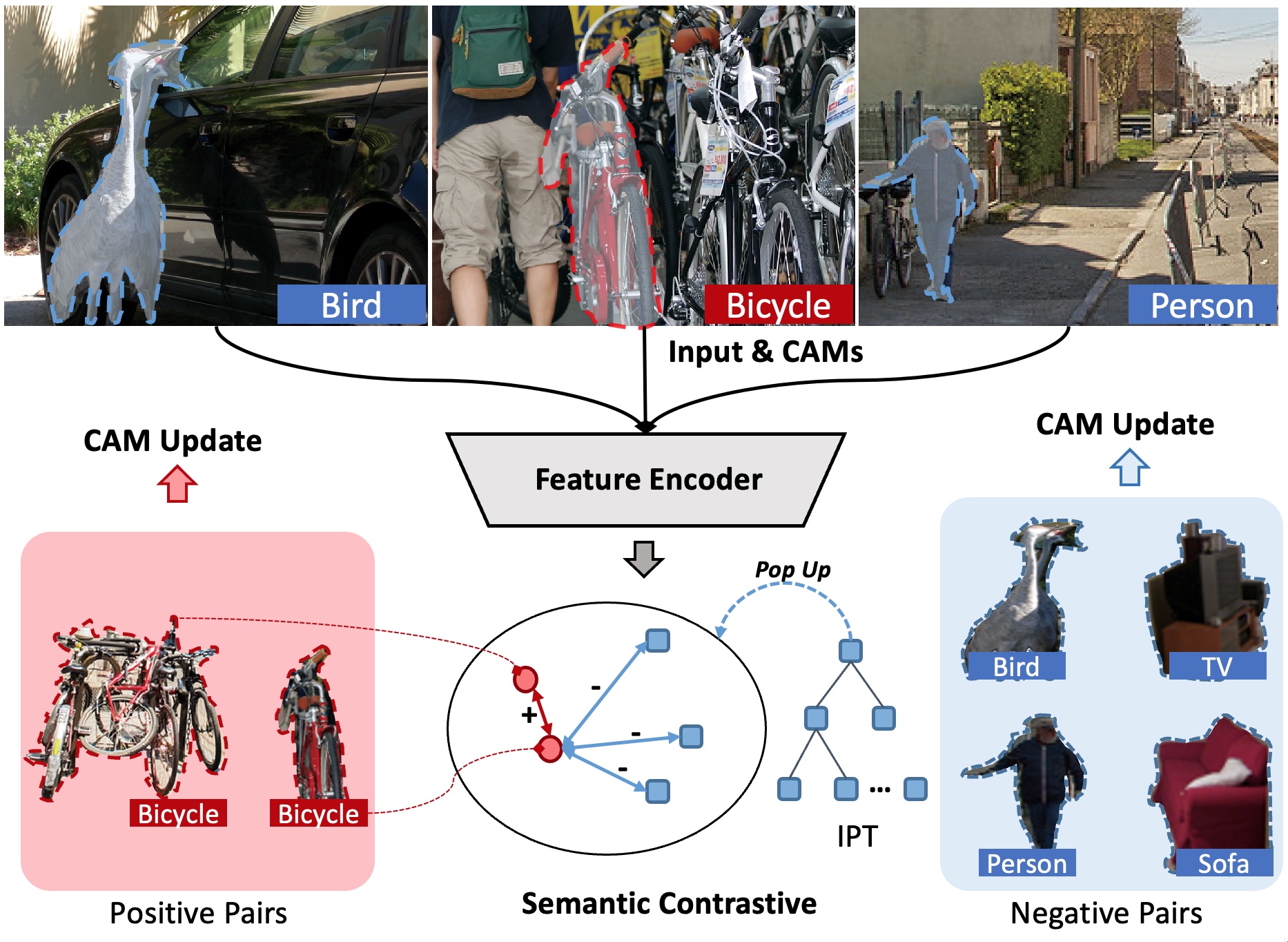
Figure 1: Illustrations of our motivation. Images usually consist of multiple semantic objects while only one is labeled. To mitigate the lack of supervision, we propose a semantic contrastive bootstrapping method that first introduces the gradient-based Class Activation Maps (CAMs) to guide the object-level feature extraction and then build semantic contrastive learning among the positive samples and negative Instance Priority Trees (IPT). To ensure the quality of CAMs, we conduct an EM-based bootstrapping optimization to iteratively update the network features (including IPT) and CAMs.

Benefiting from the strong fitting ability of deep learning systems, optimizing models with only one positive label would lead to severe negligence on indistinctive objects, while only focusing on the predominant ones. To solve this dilemma, we present a Semantic COntrastive Bootstrapping (Scob) approach, which argues to gradually recover the cross-object relationships from single-positive labels and is constructed from three aspects. i) Recent advances in Contrastive Learning (CL) approaches (Khosla et al., 2020) show that deep models have the ability to learn generalized representations without the supervision of manual labels. However, these models are invariably constrained by the discovery of image-level consistencies and discrepancies (Li et al., 2022), indicating their heavy dependencies on object-centric salient images. For multi-label learning, introducing contrastive learning intuitively would force models to learn “fake” relationships between different objects. As in Fig. 1, images only labeled with bicycle usually fail to compare with other images owing that the person plays a predominant role in feature extraction. Hence to model the object-level relationships, we introduce the gradient-based Class Activation Maps (CAM) (Chattopadhay et al., 2018) to grasp the object foreground by back-propagating the corresponding class labels, and we then encode them with a Recurrent Semantic Masked Transformer to extract spatial-aware object features in the right side of Fig. 1.

Although the proposed module shows promising benefits for feature extraction, the class activation maps trained by weak labels are usually ambiguous. Regularizing with contrastive learning would lead to accumulative errors when optimizing with such incorrect CAM initialization. On the other hand, accurate CAM guidance is also highly relied on the network training gradients, which leads to an optimization dilemma between network parameters and semantic CAM guidance. Toward this end, we ii) develop an instance priority tree to maintain a heap structure for each class, which selects the most confident objects for constructing negative samples. iii) We then propose a semantic contrastive bootstrap learning framework to iteratively update the network parameters, and CAM guidance by a generalized Expectation-Maximization model. With the proposed joint learning framework, experimental evidence demonstrates that our proposed method surpasses the state-of-the-art methods by a large margin in both single-positive and conventional partial label settings. To sum up, this paper makes the following contributions:

1. We introduce Semantic contrastive bootstrapping (Scob) to explore contrastive learning and transform representations in single-positive multi-label recognition, achieving the leading performance on public benchmarks.

2. We propose the recurrent semantic masked transformers to purify the object-level information and the instance priority tree for selecting representative negative samples.

3. We construct a bootstrap learning framework to formulate network learning and activation updating with the Expectation-Maximization model, revealing its stable convergence in weak label learning systems.

The remainder of this paper is organized as follows:  Section 2 provides the literature review and  Section 3 describes the proposed semantic contrastive bootstrapping approach. Qualitative and quantitative experimental results are reported in Section 5.  Section 6 finally concludes the paper.

2 Related Works

In this section, we first present a literature review of multi-label recognition with incomplete labels and then introduce two related techniques which are closely related to our methods, i.e., the contrastive learning and vision transformers.

2.1 Multi-Label Recognition with Incomplete Labels

Multi-label recognition is one of the most fundamental problems in computer vision society (Tsoumakas and Katakis, 2009) and has attracted increasing research attention (Chen et al., 2019b; Zhao et al., 2021; Chen et al., 2019a; Wang et al., 2016; Huynh and Elhamifar, 2020; Bucak et al., 2011; Carion et al., 2020; Wu et al., 2018; Yun et al., 2021; Guo and Wang, 2021) in recent years. However, accurate multi-label data are extremely difficult to obtain when given large sets of candidate labels or images. Recent settings on incomplete annotations have attracted much attention. In semi-supervised learning settings, several works (Zhang et al., 2021a; Balcan and Sharma, 2021) assume a subset of the training data is fully labeled while the rest is completely unlabeled. In some partial-label settings, each image is associated with a candidate set containing a correct positive label and many negatives (Gong et al., 2021; Wang et al., 2022a), whereas in others only a small percentage of labels is known for each image. To solve this problem, several works proposed to handle difficulties meeting in recognition with incomplete labels. Cole et al. (2021) propose to restore labels of the training data as distribution regularization. Shao et al. (2021) propose to learn the correlations among multi-label instances. Jiang et al. (2018) propose to clean the noise introduced by missing labels. The other line of works employ a matrix completion algorithm (Cabral et al., 2011; Xu et al., 2013; Chen et al., 2019a) to fill in the missing labels or learn the semantic features between instances and recover the missing labels by the similarity (Chen et al., 2019a, 2021; Yang et al., 2016; Pu et al., 2022). Some weakly-supervised works (Liu et al., 2018; Ge et al., 2018; Gao and Zhou, 2021; Song et al., 2021; Zhang et al., 2019) also focus on extracting object-level features to enhance the recognition or detection on labeled datasets. However, most of these methods assume that at least a certain percentage of labels is known for each training image, or additional information is provided for learning, which is usually infeasible for the commonly-used single-positive dataset.

In our work, we explore the single positive multi-label learning proposed by Cole et al. (2021), where only a single positive label is provided for each training image. The single positive label dataset can only provide very little information for multi-label classification training. To overcome it, we leverage contrastive learning to provide more information from instance disambiguation. This single positive multi-label has significant advantages to collect a large single-label dataset, which can lead to better performances (Durand et al., 2019). It is also easier for human annotators to mark the presence of only a class than notice multiple different presenting classes or what is absent from various images (Wolfe et al., 2005).

2.2 Contrastive Learning

Contrastive learning (Khosla et al., 2020) is widely used in self-supervised visual representation learning, which aims at learning representations by distinguishing different images. He et al. (2020) propose a momentum encoder and improve the negative samplings with a novel queue structure. Grill et al. (2020) propose the BYOL model further proves that it is possible to apply contrastive learning with only positive samples. Meantime, Chen et al. (2020) show that a large enough batch in the training phase is equivalent to the memory bank. Wang et al. (2022a) introduce contrastive learning to partial label learning (Gong et al., 2021). It migrates contrastive learning to mitigate label disambiguation, which is a core challenge of the task. Liu et al. (2019) leverage contrastive learning to improve the distribution of hash of different images in Hamming space. Nevertheless, these methods heavily rely on the training data to satisfy semantic consistency (Li et al., 2022) or sufficient object-central images for representation learning, which are usually infeasible in multi-label datasets. On the other hand, conventional contrastive learning methods tend to construct the generalized representation in an unsupervised manner. This learning mechanism faces a huge dilemma in discovering objects with specific semantic meanings and severely neglects the semantic information of multi-object scenarios.

Recent works also explore the unsupervised object mask with unsupervised learning, For example, DETReg (Bar et al., 2022) relies on the pre-trained agnostic object detectors DETR as coarse supervision, and FreeSOLO (Wang et al., 2022b) aims to use the predictions of pre-trained network parameters as coarse segmentation masks. Both of these methods do make contributions to focus on the main objects (i.e., relying on object-centric data), but neglect the contrastive relationship between different semantic categories, which still face great challenges in the multi-label classification tasks.

2.3 Vision Transformers

Different from CNNs with inherently limited receptive fields, Transformer (Devlin et al., 2019) is a new structure widely used in natural language processing tasks, which captures the global intrinsic features and relations with self-attention mechanism (Vaswani et al., 2017). Recent research has indicated that Transformer architectures show great potential in promoting computer vision applications. For example, Wang et al. (2021); Dosovitskiy et al. (2021a) split 2D images into a number of patches and use transformer to produce image features. Yuan et al. (2021); Liu et al. (2021); Chu et al. (2021) build new transformer suitable for vision tasks. Li et al. (2021) propose a method based on transformer for self-supervised visual representation learning. Zhao et al. (2021) use transformer to capture long-term contextual information. Transformer has also shown its successes in solving cross-modal tasks in computer vision (Shin et al., 2022). In our work, we resort to our proposed semantic mask transformer to discover object-level features and maintain the semantic consistency on multi-object images.

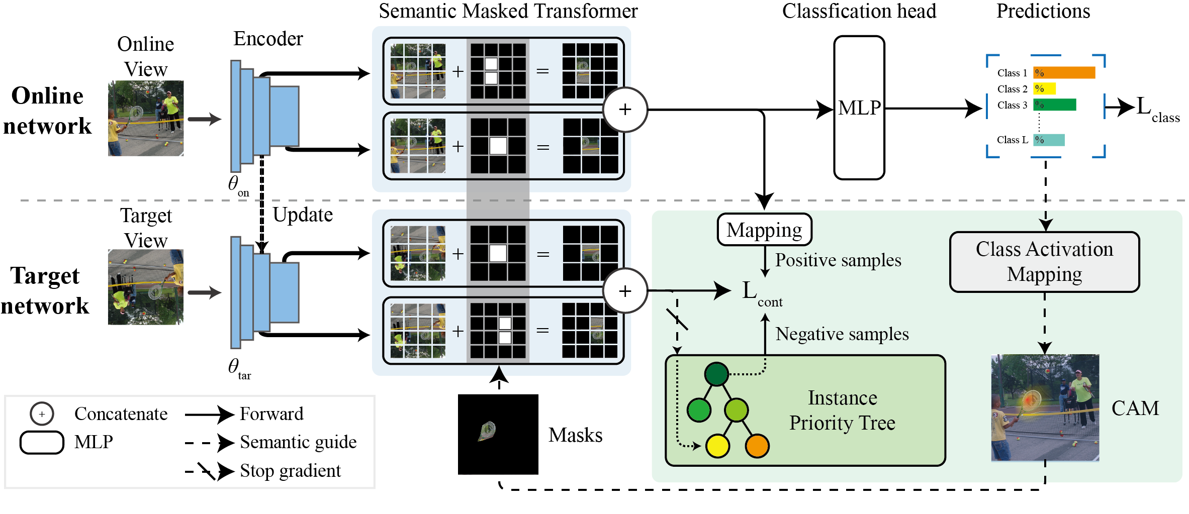
Figure 2: The pipeline of the proposed Semantic contrastive bootstrapping (Scob). Our framework first extracts the object-level class activation maps as feature extraction guidance for Semantic Masksed Transformer (SMT) and then builds a contrastive semantic relationship among the positive samples and negative samples from Instance Priority Tree (IPT). With the previously optimized networks, the object-level CAMs are then calculated by the gradient flow of ground truth labels. The overall bootstrapping framework iteratively optimizes the network parameters and object CAMs.

3 Approach

3.1 Problem Formulation

Single-positive multi-label learning Let $\mathbf{x}$ be the inputs sampled from image space $\mathcal{X}$ and $\mathbf{y}\in\{0,1\}^{L}$ be the associated full labels of input $\mathbf{x}$, where $L$ is the length of predefined label coding space $\mathcal{Y}$. In the single-positive learning, the provided annotation $\mathbf{z}$ is randomly sampled from the positive labeling space $\mathcal{Y}^{+}$. Each image is only annotated with one positive label $\mathbf{z}_{n}=1$, indicating the objects of the $n$th category exist in image $\mathbf{x}$. While $\mathbf{z}_{j}=0$ for $j=\{1,2,3,\dots,L\}\backslash\{n\}$ indicates that the other labels are unknown and could be positive or negative either. For other partial label learning settings, $\mathbf{z}\in\mathcal{Z}$ can provide more than one label for easier learning. To sum up, our objective is to find a mapping function $\mathcal{R}:\mathcal{X}\mapsto\mathcal{Z}$ with partially annotated data $\mathbf{z}\in\mathcal{Z}$ for predicting in fully labeling space $\mathcal{Y}$:

$$\arg\min_{\Theta}\mathbb{E}_{(\mathbf{x},\mathbf{y})\in\mathcal{X}\times\mathcal{Y}}\xi(\mathcal{R}(\mathbf{x};\Theta),\mathbf{y}),$$ (1)

where $\Theta$ is the model parameters for mapping function and $\xi:\{0,1\}^{L}\times\mathcal{Y}$ is the evaluation criterion e.g., mAP.

Intuitions and framework overview As aforementioned, one crucial problem caused by single-positive labeling is that most objects are not iconic or salient in images, hence directly constructing image-level relationships would introduce noisy features caused by other objects. Intuitively, we propose to build an object-level relationship instead of the image levels, which relies on two meaningful modules: 1) recurrent semantic masked transformers to extract purified object-level features; 2) contrastive representation with instance priority trees to select representative negative samples.

3.2 Recurrent Semantic Masked Transformer

As the prerequisites for constructing object-level relationships, the major motif of our model is to discover the localization of objects. As there are usually multiple objects occurring in one scenario, it would lead to a severe inductive bias for deep models confusing contextual objects related to the labeled target. For example, models would take the bicycle as a part of person objects as they are usually present simultaneously in one image. To amend this learning bias during training, we present recurrent semantic masked transformers with Class Activation Maps (CAM) to decompose clusters of multiple objects as separate identities.

As proposed in the field of natural language processing, Transformer models (Devlin et al., 2019) have the intrinsic characteristic to model the relationships of contextual information. We first split high-level features of ResNet backbones as $W\times H$ patches and then feed them into the Transformer network for modeling contextual relationships and constraining the features to concentrate on regions corresponding to object classes. Beyond this self-attention modeling manner, we then introduce the gradient-based class activations (Chattopadhay et al., 2018) as semantic masks, which are back-propagated by gradients from the last two stages of ResNet backbones. Assume the backbone feature $\mathbf{F}=\Phi(\mathbf{x};\theta_{b})\in\mathbb{R}^{HW\times K}$ is extracted from ResNet stages with parameter $\theta_{b}\in\Theta$. Hence each gradient feature map corresponded to class $c$, $\mathbf{G}^{c}\in\mathbb{R}^{H\times W}$, can be back-propagated by predicted confidence score $\mathbf{p}_{c}$. The gradient-based activation $\mathbf{G}^{c}$ can be formally presented as:

$$\mathbf{G}^{c}=\boldsymbol{\texttt{ReLU}}(\frac{1}{K}\sum_{k=1}^{K}\underbrace{\frac{1}{WH}\sum_{i=1}^{WH}\frac{\partial\mathbf{p}_{c}}{\partial\mathbf{F}^{k}_{i}}}_{\text{class-related weights}}\cdot\underbrace{\vphantom{\frac{1}{WH}\sum_{i=1}^{WH}\frac{\partial\mathbf{p}_{c}}{\partial\mathbf{F}^{k}_{i}}}\mathbf{F}^{k}}_{\text{feature map}}).$$ (2)

To avoid noisy features during this process, we only select the single-positive label to calculate class activation maps. For each location $(i,j)$, we then calculate CAMs $\mathbf{M}^{c}$ related to class $c$:

$$\mathbf{M}^{c}_{i,j} =\boldsymbol{\texttt{ind}}\left[\left(\frac{1}{l^{2}}\sum_{u=i-\lfloor\frac{l}{2}\rfloor}^{i+\lfloor\frac{l}{2}\rfloor}\sum_{v=j-\lfloor\frac{l}{2}\rfloor}^{j+\lfloor\frac{l}{2}\rfloor}\mathbf{G}^{c}_{u,v}\right)\geq\gamma_{\mathrm{cam}}\right],$$ (3)

where $l=\frac{H}{s}$ is sampled with window size $s$, $\gamma_{\mathrm{cam}}$ is the threshold hyperparameter, and $\boldsymbol{\texttt{ind}}[\cdot]$ is the indicator function, which is $1$ when condition is true, otherwise $0$. One dilemma in solving Eqns. (3) and (2) is that these activations can only be calculated after back-propagation, while at this moment the network is not forward-propagated to obtain the confidence scores $\mathbf{p}_{c}$. Hence to solve this dilemma, we introduce a recurrent scheme by using the activations of the $(t-1)$th iteration as guidance for the next forward propagation. On the other hand, inspired by the masked learning trend (He et al., 2021), we employ the masked multi-head attention mechanism to obtain object features of the $t$th iteration $\mathbf{H}_{i,j}^{c}(t)$, which are highly responded to class probabilities:

$$\begin{split}\mathbf{H}_{i,j}^{c}(t)&=\boldsymbol{\texttt{Attention}}(\mathbf{W}_{qry}\mathcal{M}(\mathbf{F}_{i,j}(t))\\ &\quad\quad,\mathbf{W}_{key}^{\top}\mathcal{M}(\mathbf{E}_{i,j}(t))^{\top})\cdot\mathbf{W}_{val}\mathbf{F}_{i,j}(t),\end{split}$$ (4)

$$\begin{split}\mathcal{M}(\mathbf{F}_{i,j}(t))&=(\mathbf{F}_{i,j}(t)+\mathbf{\mathbf{\Delta}}(i,j))\\ &\quad\quad\cdot\mathbf{(}1-\mathbf{M}^{c}_{i,j}(t-1)),\end{split}$$ (5)

where $\mathbf{W}_{\{\cdot\}}$ is the learnable attention weights and $\mathbf{\Delta}(\cdot):\mathbb{N}^{W\times H}\rightarrow\mathbb{R}^{1}$ is the learnable positional encoding. $\mathbf{M}^{c}$ has active regions, where the values are $1$, indicating the foreground, therefore we use $(1-\mathbf{M}^{c}_{i,j}(t-1))$ to mask the background information during learning process. In this manner, the extracted features $\mathbf{H}_{i,j}^{c}(t)$ in each multi-head attention show a high response to the specific semantic classes, serving as perquisites for the relationship discovery among different object instances. The detailed network implementation is elaborated in Appendix.

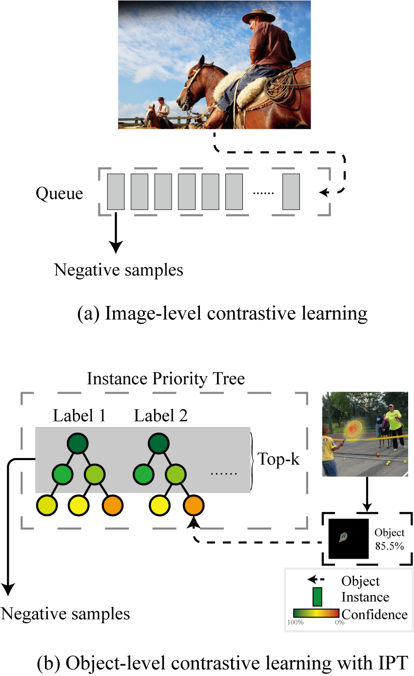
Figure 3: The contrastive learning pattern at different levels. (a) Image-level contrastive learning (He et al., 2020; Grill et al., 2020): introducing the queue structure to collect image-level instances as negative samples. (b) Our instance priority tree: the images are masked and instances are inserted into the instance priority tree with confidence. By operating the heaps, the instance priority tree always selects the most confident instances to construct the negative samples, which are used in object-level contrastive learning.

3.3 Instance Priority Tree for Contrastive Learning

Contrastive learning for multi-label recognition Recent advances (Khosla et al., 2020) in contrastive learning demonstrate that using additional contrastive constraints could help the generalization ability of model learning by alleviating overfitting issues. The main objective in prevailing contrastive learning methods is to construct positive and negative instances to learn semantic consistency across images. However, their success heavily relies on object-centric images and learning general concepts from a large amount of data, which are usually unavailable for the multi-label dataset. Hence our goal is to construct object-level relationships for contrastive learning with our proposed object-level semantics. Our contrastive architecture follows the state-of-the-art works, including MoCo (He et al., 2020) and BYOL (Grill et al., 2020), which is composed of an online network $\mathcal{T}_{on}$ and target network $\mathcal{T}_{tar}$.

Given an image $\mathbf{x}_{n}$ associated with a single-positive label $\mathbf{z}_{n}=\{0,1\}^{L}$, we randomly select the positive samples $\mathbf{x}_{t}^{+}$ from $\mathcal{X}^{+}_{n}=\{\mathbf{x}_{i};\mathbf{z}_{i}=\mathbf{z}_{n}\}_{i=1}^{N}$, and negative ones $\mathbf{x}_{t}^{-}$ from $\mathcal{X}^{-}_{n},\mathcal{X}^{-}_{n}=\mathcal{X}_{n}\backslash\mathcal{X}^{+}_{n}$ and then generate two distinctive samples by view augmentation Aug. The augmented views are then encoded with the proposed transformers to obtain feature $\widetilde{\mathbf{H}}$:

$$\widetilde{\mathbf{H}}_{on} =\mathcal{T}_{on}(\boldsymbol{\texttt{Aug}}_{o}(\mathbf{x}_{n});\theta_{on}),$$ (6)

$$\begin{split}\widetilde{\mathbf{H}}_{tar}^{\{+,-\}}&=\mathcal{T}_{tar}(\boldsymbol{\texttt{Aug}}_{t}(\mathbf{x}_{t}^{\{+,-\}});\theta_{tar}),\\ &\qquad\qquad\qquad\mathrm{where}~{}\mathbf{x}_{t}^{+}\in\mathcal{X}^{+}_{n},\mathbf{x}_{t}^{-}\in\mathcal{X}^{-}_{n}.\end{split}$$ (7)

After obtaining contrastive samples, we then attach a classification head $g$ to predict multi-label probability $\mathbf{p}_{n}$ for image $\mathbf{x}_{n}$.

Instance priority tree Constructing object-level contrastive constraint requests representative object features of each class. However, learning with weak image-level labels usually gets inferior CAMs for object localization, especially for those with co-occurrence relationships. For example, it is hard to disentangle iconic CAMs for horse and person in a riding scenario (Fig. 3 a). Hence we propose a heap structure to select representative samples from each class as negative instances for contrastive learning. As in Fig. 3 b, for each class $c$, we maintain a complete binary tree graph $\mathbb{G}=\{\mathcal{E},\mathcal{N}\}$ for selecting the samples with high confidence. Each node $\mathbf{N}$ is composed of masked semantic node feature $\widetilde{\mathbf{H}}$ with corresponding activation confidence scores $\mathbf{s}$. And each edge $e\in\mathcal{E}$ indicates an affiliation relationship where the parent node is with higher confidence than the leaf ones. To avoid noisy features, we only use the object features that are supervised by single-positive ground truth to construct the proposed tree structure.

By leveraging this tree structure, we then obtain the top-$K$ confident negative samples for each class, resulting in an affordable complexity of $\mathcal{O}(K\log N_{c})$. $N_{c}$ is the node number of the priority tree of the $c$-th class, which is much larger than the batch size. With the constructed representative samples, the contrastive InfoNCE loss (Oord et al., 2018) could be adapted as:

$$\begin{split}&\mathcal{L}_{\mathrm{cont}}(\widetilde{\mathbf{H}},\widetilde{\mathbf{H}}^{\{+,-\}},\mathcal{N})\\ &=-\lambda_{c}\frac{1}{1+\lvert\mathcal{N}\backslash\mathcal{N}^{i}\rvert}\\ &\quad\cdot\log\frac{\exp(\widetilde{\mathbf{H}}\cdot\widetilde{\mathbf{H}}^{+}/\tau)}{\exp(\widetilde{\mathbf{H}}\cdot\widetilde{\mathbf{H}}^{+}/\tau)+\sum_{\widetilde{\mathbf{H}}^{-}\in\mathcal{N}\backslash\mathcal{N}^{i}}\exp(\widetilde{\mathbf{H}}\cdot\widetilde{\mathbf{H}}^{-}/\tau)},\end{split}$$ (8)

where $\widetilde{\mathbf{H}}^{\{+,-\}}$ come from the target network indirectly, $\mathcal{N}\backslash\mathcal{N}^{i}$ are samples maintained by $\mathbb{G}$ except those labeled with $i$. $\tau$ and $\lambda_{c}$ is temperature and weighting parameter. $\widetilde{\mathbf{H}}$ is then used to update instance priority tree $\mathbb{G}$. By Eqns. (6) $\sim$ (8), our object-level contrastive learning then regularizes the network to be aware of representative object features for each class.

4 Bootstrapping Optimization with Expectation-Maximization

For each optimization tuple $(\mathbf{x},\mathbf{M},\mathbf{z})$ of the input image, CAM guidance, and observed label, one natural concern is that class activation $\mathbf{M}$ can only be obtained by prediction $\mathbf{p}$ via back-propagation processes, which can not be obtained afore the optimization. In other words, as activation $\mathbf{M}$ serves as the semantic guidance for feature extraction, a bad initialization of $\mathbf{M}$ would lead to the failure of whole learning optimization. For such a “chicken-and-egg” conundrum, we thus pursue a bootstrapping optimization with Expectation-Maximization (EM) modeling. For simplicity, if we ignore terms not depending on $\Theta$, e.g., distribution regularization, the expected log-likelihood can be defined as:

$$\begin{split}&\mathcal{Q}(\Theta^{t},\Theta^{t-1})\\ &\quad=\sum_{\mathbf{M}}\mathcal{P}(\mathbf{M}\mid\mathbf{x},\mathbf{z};\Theta^{t-1})\log\mathcal{P}(\mathbf{x},\mathbf{M};\Theta^{t}).\end{split}$$ (9)

For the hidden activation map $\hat{\mathbf{M}}$ using the $t$-1th model, we then simplify Eqns. (2) and (3) as function CAM, thus the E-step optimization on $\hat{\mathbf{M}}$ is:

$$\begin{split}\hat{\mathbf{M}}&=\arg\max_{\mathbf{M}}\mathcal{P}(\mathbf{M}\mid\mathbf{x};\Theta^{t-1})\\ &\approx\boldsymbol{\texttt{CAM}}(\frac{\partial g(\Phi(\mathbf{x};\Theta^{t-1}))}{\partial\Phi(\mathbf{x};\Theta^{t-1})}\Phi(\mathbf{x};\Theta^{t-1})),\end{split}$$ (10)

where $g(\cdot)$ denotes the classification head. Instead of directly calculating the most confidence region, we approximate $\hat{\mathbf{M}}$ by the Gradient CAM (Chattopadhay et al., 2018) via back-propagating the prediction probability $\mathbf{p}$.

In the Maximization-step of our framework, the $\mathcal{Q}$ optimization is composed of two parts,  i.e., optimization on the online network $\mathcal{Q}(\cdot;\theta_{on})$ and target network $\mathcal{Q}(\cdot;\theta_{tar})$. For the main online network, we introduce auxiliary distribution constraints to encourage the discovery of multiple objects. In each mini-batch $B$ of size $\mathrm{b}$, we denote $\mathbf{P}_{B},\mathbf{Z}_{B},\widetilde{\mathbf{Y}}_{B}\in\mathbb{R}^{b\times L}$ as predictions and labels of batch $B$, and $\mathbf{p}_{n},\mathbf{z}_{n},\widetilde{\mathbf{y}}_{n}$ indicate rows of them respectively. Following Cole et al. (2021), the single-positive multi-label classification loss is composed of three parts: 1) single-positive binary cross-entropy (BCE) $\mathcal{L}_{\mathrm{BCE}}^{+}$: only calculated with one-hot positive label $\mathbf{z}$; 2) standard BCE loss $\mathcal{L}_{\mathrm{BCE}}$: updated using the estimated multi-label $\widetilde{\mathbf{y}}_{n}$ stored in the estimator matrices; 3) distribution regularization: maintaining the averaged prediction share similarities with distributions of training data. For batch-wise predictions $\mathbf{P}_{B}$ and estimated weak label $\widetilde{\mathbf{Y}}_{B}$ which are predicted by the network and the estimator, it has the following form:

$$\begin{split}\mathcal{L}_{\mathrm{sp}}&(\mathbf{P}_{B}\mid\widetilde{\mathbf{Y}}_{B};\theta_{on})\\ &=\frac{1}{|B|}\left(\sum_{n\in B}\underbrace{\mathcal{L}_{\mathrm{BCE}}(\mathbf{p}_{n},\mathcal{S}(\widetilde{\mathbf{y}}_{n}))}_{\text{pseudo multi-label}}+\sum_{n\in B}\underbrace{\mathcal{L}_{\mathrm{BCE}}^{+}(\mathbf{p}_{n},\mathbf{z}_{n})}_{\text{ single-positive}}\right)\\ &\qquad+\underbrace{\left((\hat{k}(\mathbf{P}_{B})-k)/{L}\right)^{2}}_{\text{distribution constraint}},\end{split}$$ (11)

where $\mathcal{S}(\cdot)$ denotes the stop-gradient function and $\hat{k},k$ are the expectation of number of positive labels per image (refer to Cole et al. (2021) for details). Switching the arguments $\mathbf{F}_{B},\widetilde{\mathbf{Y}}_{B}$ and combining them, we get

$$\begin{split}&\mathcal{L}_{\mathrm{class}}(\mathbf{F}_{B},\widetilde{\mathbf{Y}}_{B};\theta_{on})\\ &\qquad=\frac{\mathcal{L}_{\mathrm{sp}}(\mathbf{F}_{B}\mid\widetilde{\mathbf{Y}}_{B};\theta_{on})+\mathcal{L}_{\mathrm{sp}}(\widetilde{\mathbf{Y}}_{B}\mid\mathbf{F}_{B};\theta_{on})}{2},\end{split}$$ (12)

where in the initialization phase of $\widetilde{\mathbf{Y}}$, we set the probability after the sigmoid function of known labels close to 1 and initialize the probability after the sigmoid of unknown labels into $u$, where $u\sim[0.5-\xi,0.5+\xi]$ and $\xi=0.3$ empirically following Cole et al. (2021). Besides the classification loss, the proposed contrastive loss $\mathcal{L}_{\mathrm{cont}}(\cdot;\theta_{on})$ in Eqn. (8) also regularizes the network after updating $\hat{\mathbf{M}}$ in the E-step. Following other contrastive learning schemes (Grill et al., 2020), the target network $\theta_{tar}$ follows momentum updating trend:

$$\theta_{tar}\leftarrow\alpha\theta_{tar}+(1-\alpha)\theta_{on},$$ (13)

where $\theta_{tar}$ and $\theta_{on}$ is the parameters of target network $\mathcal{T}_{tar}$ and online network $\mathcal{T}_{on}$, $\alpha\in[0,1)$ is a momentum coefficient. Our bootstrapping framework is elaborated in Alg. 1.

Data: Training data $\mathcal{X}$ with associated label space $\mathcal{Z}$, online network $\theta_{on}$, target network $\theta_{tar}$.

Initialize $\mathbb{G}^{c},c\in\{1,2,\dots,C\},t=0$;

Initialize $\Theta^{0}\leftarrow\boldsymbol{\texttt{optimizer}}(\Theta,\nabla_{\Theta}\mathcal{L}_{\text{class}})$;

while not convergence or $t<\boldsymbol{\texttt{MaxIter}}$ do

       for $(\mathbf{x}_{n},\mathbf{z}_{n})\sim B(\mathcal{X}\times\mathcal{Z})$ do

             $t\leftarrow t+1$ ;

             Get prediction $\mathbf{P}_{B}=g(\Phi(\mathbf{x};\Theta^{t-1}))$;

             Obtaining class activation map $\hat{\mathbf{M}}^{t-1}=\boldsymbol{\texttt{CAM}}(\mathbf{x};\Theta^{t-1})$ by Eqn. (3) ;

              /* E-Step */

              $\mathbb{G}^{\mathbf{p}_{k}}\leftarrow\mathbb{G}^{\mathbf{p}_{k}}\cup\{\mathbf{H}(\hat{\mathbf{M}}_{\mathbf{p}_{k}}),\mathbf{s}_{\mathbf{p}_{k}}\}$ by Eqn. (4) ;

             $\widetilde{\mathbf{H}}_{on}=\mathcal{T}_{on}(\boldsymbol{\texttt{Aug}}_{o}(\mathbf{x}_{n}),\hat{\mathbf{M}}^{t-1};\theta_{on})$;

             $\theta^{t}_{on}\leftarrow\boldsymbol{\texttt{optimizer}}(\theta_{on},\nabla_{\theta_{on}}\mathcal{L}_{\text{class}}(\mathbf{P},\widetilde{\mathbf{Y}}^{t-1}_{B}))$, update $\widetilde{\mathbf{Y}}_{B}^{t}$ ;

              /* M-Step */

             $\widetilde{\mathbf{H}}_{tar}^{+}=\mathcal{T}_{tar}(\boldsymbol{\texttt{Aug}}_{t}(\mathbf{x}_{t}^{+}),\hat{\mathbf{M}}^{t-1};\theta_{tar})$;

             Sample top-k negative samples from instance priority tree $\widetilde{\mathbf{H}}_{tar}^{-}\sim\mathbb{G}^{c},c\neq\mathbf{z}_{n}$ ;

             $\theta^{t}_{on}\leftarrow\boldsymbol{\texttt{optimizer}}(\theta_{on},\nabla_{\theta_{on}}\mathcal{L}_{\text{cont}}(\widetilde{\mathbf{H}}_{on},\widetilde{\mathbf{H}}_{tar}^{\{+,-\}}))$;

            

       end for

      $\theta_{tar}^{t}\leftarrow\alpha\theta_{tar}^{t-1}+(1-\alpha)\theta_{on}^{t}$ ;

        /* Target Net Updating */

      

end while

Algorithm 1 Bootstrapping Optimization with Expectation-Maximization

Table 1: mAP Comparisons (%) with the state-of-the-art methods on the VOC 2007/2012, CUB and COCO datasets. $10\%$ Pos. Neg.: training with 10% of full labels. 1 Positive: single positive setting. *: values are averaged over three runs. The best results on each dataset are highlighted in bold.

Methods	Backbone	Labels Per Image	VOC 2007	VOC 2012	CUB	Microsoft COCO
SSGRL	ResNet-101	$10\%$ Pos. Neg.	$77.7$	-	-	$62.5$
GCN-ML	ResNet-101	$10\%$ Pos. Neg.	$74.5$	-	-	$63.8$
KGGR	ResNet-101	$10\%$ Pos. Neg.	$81.3$	-	-	$66.6$
Curriculum labeling	ResNet-101	$10\%$ Pos. Neg.	$44.7$	-	-	$26.7$
Partial BCE	ResNet-101	$10\%$ Pos. Neg.	$80.7$	-	-	$61.6$
SST	ResNet-101	$10\%$ Pos. Neg.	$81.5$	-	-	$68.1$
SARB	ResNet-101	$10\%$ Pos. Neg.	$83.5$	-	-	$71.2$
ROLE	ResNet-50	$1$ Positive	-	$88.2$	$16.8$	$69.0$
Scob (Ours)*	ResNet-50	$1$ Positive	$\mathbf{88.5}$	$\mathbf{89.7}$	$\mathbf{20.4}$	$\mathbf{74.8}$
Scob (Ours)*	ResNet-50	$10\%$ Pos. Neg.	$\mathbf{88.9}$	$\mathbf{89.8}$	$\mathbf{21.4}$	$\mathbf{75.2}$

5 Experiments

5.1 Experiment Setup

Datasets Following the previous studies (Cole et al., 2021; Chen et al., 2021), we conduct experiments on four representative benchmarks, i.e., PASCAL VOC 2007 (Everingham et al., 2007), PASCAL VOC 2012 (Everingham et al., 2012), Microsoft COCO 2014 (Lin et al., 2014), CUB-200-2011 (Wah et al., 2011), which are fully labeled and widely-used in multi-label image recognition. PASCAL VOC (Everingham et al., 2012) contains $20$ categories, where each image in the dataset has $1.4$ labels on average. Microsoft COCO (Lin et al., 2014) is the most widely-used and challenging benchmark in multi-label classification tasks, which contains $80$ categories. Each image in the MS-COCO dataset contains 2.9 labels on average. It explores the object recognition task, altering the task from recognizing only the prominent object to understanding multiple objects in holistic scenarios. CUB-200-2011 (Wah et al., 2011) is the most widely-used dataset for fine-grained visual classification tasks. It has 312 binary attributes per image describing various details, which is more challenging than the first three datasets.

Baselines settings We adopt the re-implemented ROLE (Cole et al., 2021) as our baselines in the following experiments. i) While different from ROLE (Cole et al., 2021) using linear initialization, in our baseline model (i.e., Scob w/o all) all proposed modules are replaced with two convolutional layers as a simple classification head and contrastive learning is disabled in training. ii) To evaluate the effectiveness of our model, we implement the large-CNN network with more training parameters by adding convolutional blocks, which is detailed in Tab. 3.

Evaluation metrics For fair comparisons, we follow Chen et al. (2021); Cole et al. (2021); Durand et al. (2019) and adopt the mean Average Precision (mAP) as evaluation metrics. As there are few works reported their results on the single-positive setting, we compare our methods with the partial label learning methods (Chen et al., 2019a, b, 2022; Durand et al., 2019; Chen et al., 2021; Pu et al., 2022) on the $10\%$ partial label settings. that Scob is proposed in single-positive multi-label setting as aforementioned. Besides the mAP results, we additionally report average overall precision (OP), overall recall (OR), overall F1-score (OF1), per-class precision (CP), per-class recall (CR), and per-class F1-score of some approaches. For fair comparisons, we report the mean values with three random seeds, while the results of other works are reported by their original paper.

Table 2: Detailed comparisons on different evaluation metrics. The baseline model (Cole et al., 2021) is re-implemented by ours, which shows slightly higher performances.

Benchmark	Methods	Labels	OP	OR	OF1	CP	CR	CF1
PASCAL VOC 2007	Baseline (Cole et al., 2021)	$1$ Positive	$91.7$	$77.4$	$84.0$	$90.3$	$74.5$	$81.6$
	Scob (Ours)	$1$ Positive	$90.0$	$80.2$	$84.9$	$86.7$	$79.2$	$82.8$
	Scob (Ours)	$10\%$ Pos. Neg.	$87.3$	$84.4$	$85.8$	$84.4$	$82.8$	$83.6$
PASCAL VOC 2012	Baseline (Cole et al., 2021)	$1$ Positive	$85.2$	$83.3$	$84.2$	$83.9$	$81.1$	$82.5$
	Scob (Ours)	$1$ Positive	$88.2$	$82.1$	$85.0$	$84.6$	$81.7$	$83.1$
	Scob (Ours)	$10\%$ Pos. Neg.	$87.1$	$85.2$	$86.2$	$85.3$	$83.5$	$84.4$
MS COCO 2014	Baseline (Cole et al., 2021)	$1$ Positive	$70.1$	$68.3$	$69.2$	$68.0$	$63.1$	$65.5$
	Scob (Ours)	$1$ Positive	$81.1$	$66.2$	$72.9$	$78.7$	$61.1$	$68.8$
	Scob (Ours)	$10\%$ Pos. Neg.	$79.3$	$68.6$	$73.6$	$79.7$	$62.8$	$70.2$

Table 3: Ablation studies of different components. Rec. SMT: Recurrent semantic masked transformers. CL: Contrastive learning. IPT: instance priority tree for negative sampling. $/$: the proposed module is not used. $+$: the proposed module is enabled. w/o CAM: only remove CAM but retain other parts in SMT.

Rec. SMT	CL	Sampling	Parameter	mAP on MS-COCO
$/$	$/$	$/$	$36.6~{}\textrm{M}$	$69.8$
Large CNN	$/$	$/$	$45.0~{}\textrm{M}$	$70.9$
CAM	$/$	$/$	$38.3~{}\textrm{M}$	$73.8$
$/$	$+$	IPT	$36.6~{}\textrm{M}$	$68.9$
w/o CAM	$+$	Random	$38.3~{}\textrm{M}$	$73.2$
w/o CAM	$+$	IPT	$38.3~{}\textrm{M}$	$73.9$
CAM	$+$	Random	$38.3~{}\textrm{M}$	$74.3$
CAM	$+$	IPT	$38.3~{}\textrm{M}$	$\mathbf{74.8}$

5.2 Implementation Details

Data preprocessing Following the single-positive learning setting (Cole et al., 2021), we firstly drop the existing annotations of datasets and randomly retain a positive label per image. While for partial-label settings, following state-of-the-art works (Chen et al., 2021), we randomly reserve $10\%$ labels per image for a fair comparison. These operations are performed only once so that the randomly retained label is fixed for all approaches. To evaluate the performance of these approaches, we keep all the labels of the official validation sets. The results are reported on the whole validation set.

Training details We adopt ResNet-50 (He et al., 2016) pretrained on ImageNet (Deng et al., 2009) as backbone for fair comparison. The backbone can be easily replaced with other networks like ViT (Dosovitskiy et al., 2021b). Following Grill et al. (2020), images are resized into $448\times 448$ with data augmentation. Similar to Carion et al. (2020), $P$ is implemented as a self-learning positional encoding function. We adopt the Adam optimizer and train the model for $30$ epochs. The learning rates for the estimator, SMT, mapping layers, and others in the online network are $0.01$, $4\times 10^{-4}$, $0.01$, $0.001$ respectively. The batch size is set as $8$. The dimension of features is set as $512$. The hidden dimension of the transformer is set as $2048$. Each transformer unit consists of $2$ layers and each layer has $8$ attention heads. The threshold $\gamma_{\mathrm{cam}}$ is set as $0.5$. The scalar $k$ is set as $1.5$, $31.4$, and $3.0$ for VOC 2007/2012, CUB, and COCO, following Cole et al. (2021). The hyperparameters $\lambda_{c}$ is set as $0.1$. The temperature $\tau$ of contrastive learning loss is set as $1.0$. The momentum factor $\alpha$ is set as $0.999$ following Grill et al. (2020). The size of $\mathbb{G}$ is set as $80$. The backbone is frozen during training.

5.3 Comparison with State-of-The-Art Approaches

We respectively compare our approach on PASCAL VOC 2007, VOC 2012, COCO and CUB datasets with 8 state-of-the-art methods, including SSGRL (Chen et al., 2019a), GCN-ML (Chen et al., 2019b), KGGR (Chen et al., 2022), Curriculum labeling (Durand et al., 2019), Partial BCE (Durand et al., 2019), SST (Chen et al., 2021), SARB (Pu et al., 2022), and ROLE (Cole et al., 2021). As there are few works that reported their results on the single-positive setting, we also compare our methods with these aforementioned partial label learning works. However, these methods usually rely on the label-aware co-occurrence, which is corrupted for optimization in this single-positive setting. The mAP results on four benchmark datasets are exhibited in Tab. 1. It is clear that our approach achieves leader-board performance and significantly outperforms SARB (Pu et al., 2022) on both VOC and COCO by $5.8\%$ and $4.1\%$, ROLE (Cole et al., 2021) by $1.6\%$ (VOC 2012) and $5.8\%$ (COCO). Moreover, our approach achieves much higher performance than these leading works by only leveraging much fewer annotations (1 Positive) than those with $10\%$ partial labels. With the increase of annotation in the last two rows, our proposed method shows a notable improvement, verifying the robustness and effectiveness of different propositions of incomplete data annotations.

Besides the most widely-used mAP, we report average overall precision (OP), overall recall (OR), overall F1-score (OF1), per-class precision (CP), per-class recall (CR), and per-class F1-score of the baseline (Cole et al., 2021) and Scob on three datasets in Tab. 2. Considering the compared methods in the partial label learning or single-positive learning setting do not report values on these metrics, we re-implement the state-of-the-art model ROLE (Cole et al., 2021), which performs slightly higher results than the paper reports.

5.4 Performance Analyses

Effect of recurrent Semantic Masked Transformers (SMT) To ablate SMT, we replace it with several 2D convolutional layers for setting w/o SMT. From Tab. 3, we can observe that SMT notably improves the performance by incorporating a self-attention mechanism with reasonable masked semantic guidance compared to the baseline, i.e., from 69.8 to 73.8. By only removing the CAM guidance in SMT (shown in the sixth row), the overall performance decreases by $0.9\%$. This indicates that semantic guidance plays an important role in learning object-level relationships.

To validate our proposed method is mainly improved by additional parameters. In the second row, we also train a large-CNN as aforementioned that has much more parameters than ours without contrastive learning and observe that the effect of additional parameters on the performance is very limited, which further clarifies that the improvement is not just due to the additional parameters, but the cooperation of proposed new modules and object-level contrastive learning.

Different variants of contrastive regularization In Tab. 3, our full model substantially outperforms the third row without contrastive learning, which shows the effectiveness of learning object-level contrastive representation. Moreover, the performance of Scob w/o IPT decreases by $0.5\%$, in which a random sampling strategy equivalent to the vanilla memory bank used in MoCo (He et al., 2020) is applied, indicating that Instance Priority Tree (IPT) provides notable improvements with representative negative object samples. Contrastive learning helps the framework learn better representations of different labels by object disambiguation. It has been observed that networks can predict random labels, but the same network can fit informative data faster (Cole et al., 2021). Better representations let the model fit single positive data during training, recovering better weak labels.

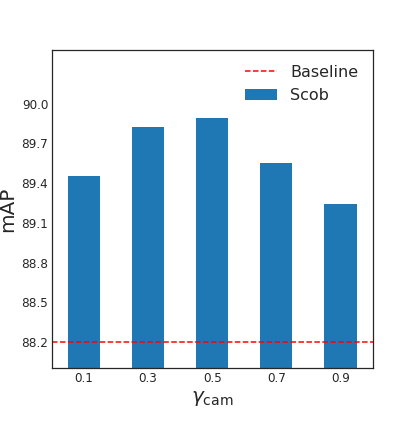
Figure 4: mAP performance on VOC12 dataset with different CAM threshold $\gamma_{\mathrm{cam}}$.

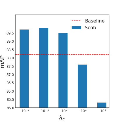
Figure 5: mAP performance on VOC12 dataset with different contrastive learning coefficient $\lambda_{c}$.

Table 4: Ablations to different contrastive learning and object detection-based methods. mAP performance on MS-COCO dataset is reported.

Methods	mAP on MS-COCO
Baseline	$69.8~{}{\color[rgb]{.5,.5,.5}(+0.0)}$
$+$BYOL	$65.5~{}{\color[rgb]{1,0,0}(-4.3)}$
$+$MoCo	$61.6~{}{\color[rgb]{1,0,0}(-8.2)}$
$+$SimCLR	$64.9~{}{\color[rgb]{1,0,0}(-4.9)}$
$+$Detco	$61.2~{}{\color[rgb]{1,0,0}(-8.6)}$
$+$SoCo	$58.2~{}{\color[rgb]{1,0,0}(-11.6)}$
$+$UP-DETR	$69.2~{}{\color[rgb]{1,0,0}(-0.6)}$
Scob (Ours)	$\mathbf{74.8}~{}{\color[rgb]{0.375,0.6953125,0.33984375}(+5.0)}$

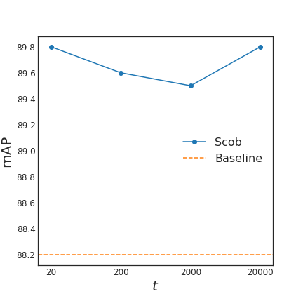
Figure 6: mAP on VOC12 of our method Scob and Baseline with different $t$ values.

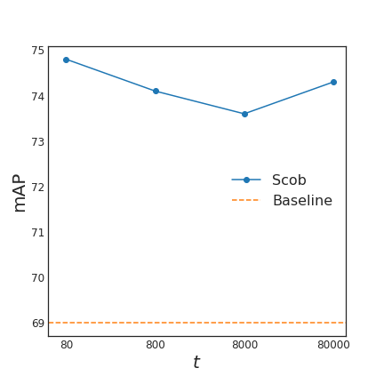
Figure 7: mAP on MS-COCO dataset of our method Scob and Baseline with different $t$ values.

Table 5: Ablations to semantic masks on VOC 2012 and MS-COCO dataset.

Datasets	Methods	mAP	OP	OR	OF1	CP	CR	CF1
VOC 2012	Baseline	$88.2~{}(+0.0)$	85.2	83.3	84.2	83.9	81.1	82.5
	GT Masks	$\mathbf{90.0}~{}{\color[rgb]{0.375,0.6953125,0.33984375}(+1.8)}$	86.2	86.2	86.2	83.9	84.9	84.4
	CAMs	$89.8~{}{\color[rgb]{0.375,0.6953125,0.33984375}(+1.6)}$	88.2	82.1	85.0	84.6	81.7	83.1
MS COCO	Baseline	$69.8~{}(+0.0)$	70.1	68.3	69.2	68.0	63.1	65.5
	GT Masks	$\mathbf{74.8}~{}{\color[rgb]{0.375,0.6953125,0.33984375}(+5.0)}$	79.0	68.4	73.3	78.8	63.2	70.1
	CAMs	$\mathbf{74.8}~{}{\color[rgb]{0.375,0.6953125,0.33984375}(+5.0)}$	81.1	66.2	72.9	78.7	61.1	68.8

Ablations to other contrastive learning and detection-based methods We replace our Scob with prevailing contrastive learning, BYOL (Grill et al., 2020), MoCo (He et al., 2020), SimCLR (Chen et al., 2020), Detco (Xie et al., 2021a), SoCo (Xie et al., 2021b), and object detection-based methods UP-DETR (Dai et al., 2021) in Tab. 4. The baseline is taken from the w/o all setting in Tab. 3, which is trained without contrastive learning. As shown in the Tab. 4, other contrastive learning methods lead to sharp performance drops compared to our approach. To compare with Detco (Xie et al., 2021a), SoCo (Xie et al., 2021b), we adopt their official pre-trained model of the MS-COCO dataset and fine-tune these models following the same baseline, i.e., ROLE (Cole et al., 2021). Although these methods provide a satisfactory representation of object detection but rely on different contrastive manners compared to ours. We focus on the contrastive learning of semantic views with CAMs to preserve the extraction of holistic objects. While Detco and SoCo focus on the relationship between local patches or cropped local views without the semantic constraints. The different focuses make the learned representations suitable for different tasks, i.e., recognition and detection. The other reason is that our Scob constructed an instance priority tree for adaptively selecting negative CAMs, while Detco and SoCo follow a common contrastive trend with negative image-level representations or simply omit this relationship.

Considering that multi-label images usually contain multiple semantic objects, data augmentations used in them constantly include random cropping to create multiple views of the original images, which may unexpectedly focus on different objects in multi-label learning, introducing wrong positive or negative samples. The wrong samples make the contrastive learning fail and mislead models to distinguish objects by the wrong features, which is the main reason for the performance drops. In our scheme, we resort to object-level representation for building contrastive learning. It selects semantic objects from images with CAM guidance instead of direct data augmentation, which tackles the problem of semantic inconsistency in multi-label learning and improves the generalization ability of network models.

Effect of different ratios $\gamma_{\textrm{cam}}$ of semantic mask As important guidance to semantic learning, we validate different ratios $\gamma_{\textrm{cam}}$ of Eqn. (3) in Fig. 4. This parameter determines how responsive the mask guidance is to the activation maps of objects. A larger value can make the mask guidance filter more unrelated to noisy context, while also requiring the masked objects to be more typical. With the increase of the threshold, the mask guidance has the potential to focus on the main object better, while the thresholds larger than $0.5$ would lead to incomplete object understanding during training, especially when the model is not so confident about the recognized objects in the early steps.

Table 6: Comparisons of different optimization methods on MS-COCO dataset. Higher results are viewed in bold.

Methods	mAP	OP	OR	OF1	CP	CR	CF1
Baseline	$69.8~{}(+0.0)$	70.1	68.3	69.2	68.0	63.1	65.5
Joint Optim.	$69.7~{}{\color[rgb]{1,0,0}(-0.1)}$	75.7	65.8	70.4	72.8	59.7	65.6
Two Stage	$74.2~{}{\color[rgb]{0.375,0.6953125,0.33984375}(+4.3)}$	75.4	70.9	73.1	75.4	64.9	69.8
Scob (Ours)	$\mathbf{74.8}~{}{\color[rgb]{0.375,0.6953125,0.33984375}(+5.0)}$	81.1	66.2	72.9	78.7	61.1	68.8

Ablation to loss weight $\lambda_{c}$ For the contrastive loss weight $\lambda_{c}$ on term $\mathcal{L}_{\mathrm{cont}}$, we conduct different parameter settings with different numbers of magnitude, while this hyperparameter can also be jointly defined by adjusting the learning rate in the contrastive learning phase. As in Fig. 5, when the contrastive learning weight $\lambda_{c}$ increases to a proper weight, i.e., $0.1$, the performance shows a slight improvement. However, exaggerating the effects of contrastive loss would override the main objective of multi-label classification and then lead to inaccurate CAM guidance. Note that in this paper we do not need to carefully tune these hyperparameters but validate their effectiveness under diverse scenarios of multiple datasets.

Ablation to the number of negative samples in contrastive learning We validate the effect of the number of negative samples in contrastive learning. Here we present results in Fig. 7 on the VOC dataset and Fig. 7 on MS-COCO dataset, where the baseline result is exhibited in the orange dotted line. We select the Top-$1$, Top-$10$, Top-$100$, and Top-$1000$ confident instances in each class following the algorithms of IPT. The curves on different datasets show similar variation tendencies that selecting the most representative samples of each class would benefit the final performance while selecting more than 8,000 samples for the MS-COCO dataset would lead to a performance drop of over $1\%$. Counter-intuitively, when increasing the number of instances with sufficient training instances, i.e., 80,000 samples in MS-COCO, the network has the potential to understand the object representations with a performance improvement. However, constraining the network to recognize a sufficiently large number of negative samples will result in a heavy computation burden, i.e., 1000$\times$ sample numbers for learning. Hence, in the trade-off between computational resources and performances, we respectively use $20$ and $80$ negative samples on VOC and MS-COCO datasets, by selecting the most confident instances in each class.

Semantic CAMs vs. ground truth masks To understand the influence brought by semantic masks of different qualities, we modify the CAM guidance with the ground truth segmentation masks. In order to migrate the segmentations to our tasks, for ground truth, labels are dropped and a single positive label is retained. Next, we only keep segmentation masks that contain the objects belonging to the single positive label and ignore other segmentation annotations. The segmentation masks are resized with max pooling to generate masks while fitting the shape of the features. The experimental results of Scob with CAM and ground truth on the two benchmark datasets are listed in Tab. 5. It is interesting that the gap in mAP evaluations is relatively small, i.e., less than 0.2%, demonstrating that the CAM selected by IPT is of high quality in contrastive learning. We also conduct detailed analyses with six other evaluation metrics in Tab. 5. Models with generated CAMs show a higher overall precision (OP) but with lower overall recall (OR) compared to the models with GT masks. This implies that the GT masks can activate more features of positive classes for the final classification but meanwhile introduces additional noisy features for classification.

Table 7: CAM evaluations on feature space of different variants on the VOC training set.

Methods	Precision	Recall	F1-Score
Scob w/o CL	48.1	63.3	54.7
Scob w/ CL	50.0	68.2	57.7

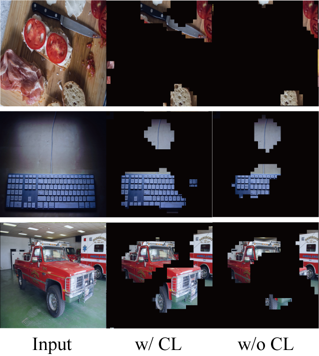
Figure 8: Visualization of semantic masks on MS-COCO. Each group of images from left to right are original image, Scob and Scob w/o CL respectively.

Effect of EM-based Bootstrapping To verify the effectiveness of the proposed EM-based bootstrapping, we conduct experiments with two different alternatives.

1. Joint Optimization: training the network parameters $\Theta$ and object CAMs $\mathbf{M}$ simultaneously.

2. Two Stage: training network without CAM guidance $\mathbf{M}$ in the first 10 epochs and then conducting the proposed EM-based bootstrapping in the next 20 epochs.

In Tab. 6, the joint optimization shows similar performance with the baseline models while remaining a gap (5.1 in mAP) with the proposed EM-based bootstrapping model. This indicates the inferior initialization of CAMs and network parameters would harm the optimization process and cannot be fully corrected during learning. Results in the third row denote this two-stage training manner, which shows a clear performance increase (+4.3%) compared to the baseline models, but still lower than the proposed EM bootstrapping training scheme. From Tab. 6, the method without using CAMs in the initial training phase (i.e., Two stage) would lead to a clear performance drop in overall precision (OP) but with higher recalls (OR).

Table 8: Comparisons of inference speed (per image) and performance on MS-COCO dataset.

Methods	Speed	Settings	mAP
Baseline (Cole et al., 2021)	$7.67ms$	1-positive	69.8
SST (Chen et al., 2021)	$19.84ms$	10% partial	68.1
SARB (Pu et al., 2022)	$19.09ms$	10% partial	71.2
Scob (Ours)	$12.14ms$	1-positive	74.8

Time efficiency In Tab. 8, we conduct experiments to compare the evaluation speed on a single NVIDIA 3090 GPU with the input resolution of $448\times 448$. The baseline model (Cole et al., 2021) without any additional modules shows a fast inference speed of 7.67ms per image. Compared to recent works i.e., SST (Chen et al., 2021), SARB (Pu et al., 2022), our proposed method achieves a good trade-off with notable performance improvement and acceptable time costs.

5.5 Visualization Analyses

Visualizations of semantic masks In Fig. 8, we visualize the instances produced by Scob (second column) and Scob w/o contrastive learning (third column). We can observe that the semantic masks generated with contrastive learning show clear silhouettes, focuses more on the semantic objects, and mitigates the influence of other contextual objects, e.g., discovering knife out of other foods in the first row. We have also conducted a detailed comparison of CAMs with ground truth segmentation masks in the feature space, as in Tab. 7. By adding the contrastive learning on CAMs, the F1-score has improved by 3.0% with clearer localizations. Object-level contrastive learning distinguishes different instances in multi-object images and improves the recognition performance. Besides, we also exhibit more visualization results related to specific categories in Fig. 10 of our Appendix.

Distributions of unknown predictions Here we present the distribution of predicted probabilities for unknown negatives on single-positive COCO in Fig. 9, which are the major parts of unknown labels. During training stages, Scob fast predicts more accurate negative labels. The predicted probabilities by our approach of ground-truth negatives show a quick convergence to the $0$ side, while the probability distribution predicted by ROLE (Cole et al., 2021) is dispersed. This indicates that due to the new module and contrastive learning, the model obtains more knowledge during training, and learns more representative features to distinguish the differences between objects so that the non-existent objects can be eliminated faster, which improves the overall performance.

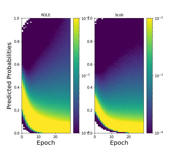
Figure 9: Distribution of predicted probabilities for unknown negatives by ROLE (left) and Ours (right) on single-positive COCO. Each pixel stands for histograms, indicating a frequency from $1.0$ (yellow) to $0.0$ (blue) of the specific confidence value.

6 Conclusions and Limitations

In this paper, we focus on the problem of multi-label image recognition with single-positive incomplete annotations. To this end, we argue to use a gradient-based class activation map from the previous step as guidance and propose a semantic contrastive bootstrapping learning framework to iteratively refine the guidance and label predictions. In this framework, we propose a recurrent semantic masked transformer to extract accurate clear object-level features and a contrastive constraint with instance priority trees for building cross-object relationships. Experimental results verify our proposed method achieves superior performance compared to state-of-the-art methods.

As our proposed method is a weakly-supervised learning method, it still faces problems when discovering the full ground truth annotations, which limits the performance compared to the fully-supervised methods. Besides, on the fine-grained multi-label learning with extremely limited labels, prevailing techniques including our method remain space for further exploration, including investigating fine-grained local parts instead of the holistic objects, which we would like to investigate in our future work.

Appendix

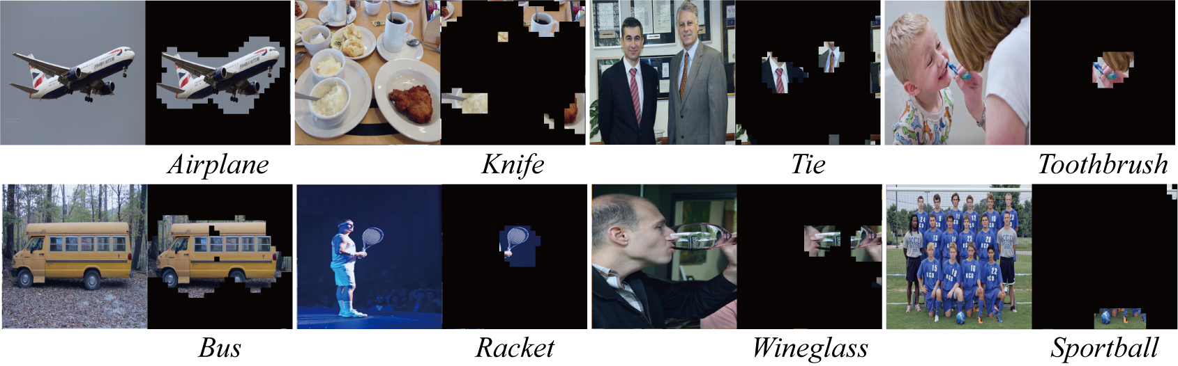
Figure 10: Visualization of semantic masks on MS-COCO. In each group, the left and right images denote the input image and the masked class activation maps in our proposed Scob approach.

A. Visualizations on Class-specific Semantic Masks

Beyond the ablations on semantic masks in the main manuscript, here we exhibit more semantic masks generated on the MS-COCO dataset in Fig. 10. In each group, the left and right images denote the input image and the masked class activation maps in our proposed Scob approach. As in the first two columns, it can be found that our proposed approach focuses on the semantic objects e.g., airplane and bus, while filtering the background information. In the second to the fourth groups of Fig. 10, two major challenges occur to distinguish these objects: 1) the semantic objects are relatively small compared to the image size; 2) these objects show high dependencies on the other objects or namely co-occurrences. As can be seen from this generated semantic guidance, our proposed Scob has the ability to distinguish the specific object from its related objects and then forms the representative features.

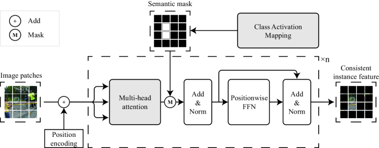
Figure 11: The network architecture of the proposed Recurrent Semantic Masked Transformer. We leverage the masked multi-head attention mechanisms with iterative semantic guidance generated by CAMs.

B. Performances on Recognizing Small Objects

Besides Fig. 10 showing some CAM results of large and small-scale objects. We additionally list the AP results of 10 small-scale classes in the MS-COCO dataset to show our approach is robust to them in Tab. 9.

Table 9: The AP results of 10 small-scale classes in MS-COCO dataset.

#	Classes	AP
1	banana	$93.0$
2	baseball bat	$76.0$
3	baseball glove	$80.9$
4	book	$70.8$
5	mouse	$74.6$
6	remote	$84.3$
7	scissors	$86.1$
8	stop sign	$84.6$
9	tie	$88.4$
10	toothbrush	$82.4$

C. Details on Recurrent Semantic Masked Transformer

The proposed recurrent Semantic Masked Transformer (SMT) mainly consists of positional encoding, semantic mask, and multiple multi-head attention units as in previous work (Vaswani et al., 2017). Different from the implementation of these works, we rely on the feature maps of ResNet backbones as image feature patches (illustrated as image patches for a better view). Inspired by the masked coding manner (Devlin et al., 2019) in the field of natural language processing, here we adopt the class activation generated from the last optimization as the guidance for semantic masked attention. We present the detailed network architectures in Fig. 11.

Semantic masked encoding Denote $\mathbf{F}=\Phi(\mathbf{x};\theta_{b})\in\mathbb{R}^{HW\times K}$ as the backbone feature extracted from ResNet stages with parameter $\theta_{b}\in\Theta$. $\mathbf{F}$ is split into $H\times W$ patches $\left\{\mathbf{F}_{i,j}\mid i\in\{1,2,\dots,H\},j\in\{1,2,\dots,W\}\right\}$ of which each patch has channel size $K$, as the input of SMT. As mentioned in Section 3.2, the recurrent SMT applies a learnable positional encoding $\Delta(\cdot):\mathbb{N}^{W\times H}\mapsto\mathbb{R}^{1}$ and semantic mask to $\{\mathbf{F}_{i,j}\}$:

$$\mathcal{M}(\mathbf{F}_{i,j})=(\mathbf{F}_{i,j}+\Delta(i,j))\cdot(1-\mathbf{M}^{c}),$$ (14)

where the symbols are described as aforementioned. The implementation of $\Delta$ follows the previous Transformer architecture, i.e., DETR (Carion et al., 2020). Let $\Delta_{h}:\mathbb{N}^{W}\mapsto\mathbb{R}^{1}$ and $\Delta_{v}:\mathbb{N}^{H}\mapsto\mathbb{R}^{1}$ be the horizontal and vertical encoding. Then $\Delta$ is the concatenation of them:

$$\Delta(i,j)=\Delta_{h}(i)\oplus\Delta_{v}(j),$$ (15)

where $\oplus$ denotes the feature concatenation operation. Following Devlin et al. (2019), positional encoding and masks are applied to the query and key of multi-head attention, providing global position information and constraining the extracted features $\mathbf{H}_{i,j}^{c}$ showing high response to only a specific semantic class related to the masks.

Multi-scale SMTs As the different network stages during training are sensitive to semantic objects of different scales, hence incorporating multi-scale and multi-level features can be beneficial for final feature representations, which is also one of the challenging problems in multi-label classification tasks. In our implementation, we propose to use two SMTs connecting to Stage 3 and Stage 4 of ResNet-50, and combine their outputs to extract image features at multiple scales. In this manner, objects of small scales are more easily to be presented in earlier network stages without a significant loss in resolutions.

Data: IPT $\mathbb{G}^{i}=(\mathcal{E}^{i},\mathcal{N}^{i}),i\in\{1,2,3,\dots,L\}$, new node $v$ associated with label $z$.

/* Insert activated node $v$. */

$\mathcal{N}^{z}\leftarrow\mathcal{N}^{z}\cup\{v\}$;

/* Adjust priority tree. */

$i\leftarrow|\mathcal{N}^{z}|-1$;

Choose elements $[u_{0},u_{1},u_{2},\dots,u_{n}]$ in $\mathcal{N}^{z}$;

while $i>0~{}\textbf{and}~{}s_{\lfloor i/2\rfloor}<s_{i}$ do

       Swap $u_{\lfloor i/2\rfloor}$ and $u_{i}$;

       $i\leftarrow\lfloor i/2\rfloor$;

      

end while

Adjust $\mathcal{N}^{z}$ by removing exceed nodes from the end of it;

Algorithm 2 Insert activated node $v$ to $\mathbb{G}$ and adjust priority tree

Data: IPT $\mathbb{G}^{i}=(\mathcal{E}^{i},\mathcal{N}^{i}),i\in\{1,2,3,\dots,L\}$, positive label $z$, number of negative samples $t$.

Result: Negative samples $\mathcal{N}^{\prime}$.

if $i=z$ then

       $\mathcal{N}^{\prime}\leftarrow\{\}$;

       return;

      

end if

Choose elements $[u_{0},u_{1},u_{2},\dots,u_{n}]$ in $\mathcal{N}^{i}$;

if $|\mathcal{N}^{z}|<=t$ then

       /* If the size of $\mathcal{N}^{z}$ is less than $t$, simply construct samples with all nodes. */

       $\mathcal{N}^{\prime}\leftarrow\mathcal{N}^{z}$;

      

else

       /* Pop top elements $t$ times to construct samples. */

       $\mathcal{N}^{\prime}\leftarrow\{\}$;

      

      for $i\leftarrow 1$ to $t$ do

             $j\leftarrow 0$;

             Swap $u_{j}$ and $u_{n}$;

             while $2j<|\mathcal{N}^{z}|$ do

                   if $s_{2j}>s_{2j+1}$ then

                         Swap $u_{j}$ and $u_{2j}$;

                         $j\leftarrow 2j$;

                        

                  else

                         Swap $u_{j}$ and $u_{2j+1}$;

                         $j\leftarrow 2j+1$;

                        

                   end if

                  

             end while

            $\mathcal{N}^{\prime}\leftarrow\mathcal{N}^{\prime}\cup\{u_{j}\}$;

             $\mathcal{N}^{z}\leftarrow\mathcal{N}^{z}\backslash\{u_{n}\}$;

            

       end for

      /* Restore the original $\mathcal{N}^{z}$ for future operations. */

       Insert $\mathcal{N}^{\prime}$ into $\mathcal{N}^{z}$;

      

end if

Algorithm 3 Pop top nodes $\mathcal{N}^{\prime}$ from $\mathbb{G}^{i}$ for negative sampling

E. Algorithms of Instance Priority Trees

Instance Priority Tree (IPT) $\mathbb{G}=\{\mathcal{E},\mathcal{N}\}$ is a heap implemented with a complete binary tree structure, maintaining high confident instances to construct negative samples for contrastive learning. Each element $u\in\mathcal{N}$ is a binary tuple $(\widetilde{H}_{u},s_{u})$, where $\widetilde{H}_{u}$ is a semantic masked feature and $s_{u}$ is the corresponding activation confidence score. Each edge $e\in\mathcal{E}$ indicates an affiliation relationship $(u,v)$ where the parent node $u$ is with higher confidence than the leaf ones $v$.

In our implementations, we adopt an array of length $n$, $[u_{0},u_{1},u_{2},\dots,u_{n}]$, to store the nodes $\mathcal{N}$ and describe the edges $\mathcal{E}$ by their indices in the array, i.e., $u_{i}$ is the parent node of $u_{2i}$ and $u_{2i+1}$. The success of IPT relies on three typical operations: “Insert activated nodes”, “Adjust priority tree”, and “Pop top nodes”. In our implementation, the tree adjustment operation needs to be conducted after every Insert or Pop operation for maintaining the tree structures. In other words, the “Insert activated nodes” and “Adjust priority tree” functions are operated together. Here we elaborate the detailed algorithms in Alg. 2 and Alg. 3.

In addition, we maintain the size of instance priority tree $\mathbb{G}$ in a proper range to reduce computation costs. In this manner, instances with lower confidence features would not be added to our tree storage, indicating the efficiency of our model.

Data Availability Statement

The datasets generated during and/or analyzed during the current study are available in the original references, i.e., PASCAL VOC 2007/2012 (Everingham et al., 2012) http://host.robots.ox.ac.uk/pascal/VOC/, Microsoft COCO 2014 (Lin et al., 2014) https://cocodataset.org/, CUB-200-2011 (Wah et al., 2011) https://www.vision.caltech.edu/datasets/cub_200_2011/. The source codes and models corresponding to this study are publicly available.

References

- Balcan and Sharma (2021) Balcan MFF, Sharma D (2021) Data driven semi-supervised learning. In: Advances in Neural Information Processing Systems (NeurIPS)
- Bar et al. (2022) Bar A, Wang X, Kantorov V, Reed CJ, Herzig R, Chechik G, Rohrbach A, Darrell T, Globerson A (2022) Detreg: Unsupervised pretraining with region priors for object detection. In: Proceedings of the IEEE/CVF Conference on Computer Vision and Pattern Recognition, pp 14605–14615
- Bucak et al. (2011) Bucak SS, Jin R, Jain AK (2011) Multi-label learning with incomplete class assignments. In: 2011 IEEE Conference on Computer Vision and Pattern Recognition (CVPR), DOI 10.1109/CVPR.2011.5995734
- Cabral et al. (2011) Cabral R, Torre F, Costeira JP, Bernardino A (2011) Matrix completion for multi-label image classification. In: Advances in Neural Information Processing Systems (NeurIPS)
- Carion et al. (2020) Carion N, Massa F, Synnaeve G, Usunier N, Kirillov A, Zagoruyko S (2020) End-to-end object detection with transformers. In: European Conference on Computer Vision (ECCV), DOI 10.1007/978-3-030-58452-8“˙13
- Chattopadhay et al. (2018) Chattopadhay A, Sarkar A, Howlader P, Balasubramanian VN (2018) Grad-cam++: Generalized gradient-based visual explanations for deep convolutional networks. In: 2018 IEEE Winter Conference on Applications of Computer Vision (WACV), DOI 10.1109/WACV.2018.00097
- Chen et al. (2019a) Chen T, Xu M, Hui X, Wu H, Lin L (2019a) Learning semantic-specific graph representation for multi-label image recognition. In: Proceedings of the IEEE/CVF International Conference on Computer Vision (ICCV)
- Chen et al. (2020) Chen T, Kornblith S, Norouzi M, Hinton G (2020) A simple framework for contrastive learning of visual representations. In: Proceedings of the 37th International Conference on Machine Learning (ICML)
- Chen et al. (2021) Chen T, Pu T, Wu H, Xie Y, Lin L (2021) Structured semantic transfer for multi-label recognition with partial labels. arXiv preprint arXiv:211210941 DOI 10.48550/ARXIV.2112.10941
- Chen et al. (2022) Chen T, Lin L, Chen R, Hui X, Wu H (2022) Knowledge-guided multi-label few-shot learning for general image recognition. IEEE Transactions on Pattern Analysis & Machine Intelligence
- Chen et al. (2019b) Chen ZM, Wei XS, Wang P, Guo Y (2019b) Multi-label image recognition with graph convolutional networks. In: Proceedings of the IEEE/CVF Conference on Computer Vision and Pattern Recognition (CVPR)
- Chu et al. (2021) Chu X, Tian Z, Wang Y, Zhang B, Ren H, Wei X, Xia H, Shen C (2021) Twins: Revisiting the design of spatial attention in vision transformers. In: Advances in Neural Information Processing Systems (NeurIPS)
- Cole et al. (2021) Cole E, Mac Aodha O, Lorieul T, Perona P, Morris D, Jojic N (2021) Multi-label learning from single positive labels. In: Proceedings of the IEEE/CVF Conference on Computer Vision and Pattern Recognition (CVPR)
- Dai et al. (2021) Dai Z, Cai B, Lin Y, Chen J (2021) Up-detr: Unsupervised pre-training for object detection with transformers. In: Proceedings of the IEEE/CVF Conference on Computer Vision and Pattern Recognition (CVPR), pp 1601–1610
- Deng et al. (2009) Deng J, Dong W, Socher R, Li LJ, Li K, Fei-Fei L (2009) Imagenet: A large-scale hierarchical image database. In: Proceedings of the IEEE/CVF Conference on Computer Vision and Pattern Recognition (CVPR)
- Devlin et al. (2019) Devlin J, Chang M, Lee K, Toutanova K (2019) BERT: pre-training of deep bidirectional transformers for language understanding. In: Proceedings of the 2019 Conference of the North American Chapter of the Association for Computational Linguistics: Human Language Technologies
- Dosovitskiy et al. (2021a) Dosovitskiy A, Beyer L, Kolesnikov A, Weissenborn D, Zhai X, Unterthiner T, Dehghani M, Minderer M, Heigold G, Gelly S, Uszkoreit J, Houlsby N (2021a) An image is worth 16x16 words: Transformers for image recognition at scale. In: International Conference on Learning Representations
- Dosovitskiy et al. (2021b) Dosovitskiy A, Beyer L, Kolesnikov A, Weissenborn D, Zhai X, Unterthiner T, Dehghani M, Minderer M, Heigold G, Gelly S, Uszkoreit J, Houlsby N (2021b) An image is worth 16x16 words: Transformers for image recognition at scale. In: International Conference on Learning Representations
- Durand et al. (2019) Durand T, Mehrasa N, Mori G (2019) Learning a deep convnet for multi-label classification with partial labels. In: Proceedings of the IEEE/CVF Conference on Computer Vision and Pattern Recognition (CVPR)
- Everingham et al. (2007) Everingham M, Van Gool L, Williams CKI, Winn J, Zisserman A (2007) The PASCAL Visual Object Classes Challenge 2007 (VOC2007) Results. http://www.pascal-network.org/challenges/VOC/voc2007/workshop/index.html
- Everingham et al. (2012) Everingham M, Van Gool L, Williams CKI, Winn J, Zisserman A (2012) The PASCAL Visual Object Classes Challenge 2012 (VOC2012) Results. http://www.pascal-network.org/challenges/VOC/voc2012/workshop/index.html
- Gao and Zhou (2021) Gao BB, Zhou HY (2021) Learning to discover multi-class attentional regions for multi-label image recognition. IEEE Transactions on Image Processing 30:5920–5932
- Ge et al. (2018) Ge W, Yang S, Yu Y (2018) Multi-evidence filtering and fusion for multi-label classification, object detection and semantic segmentation based on weakly supervised learning. In: Proceedings of the IEEE Conference on Computer Vision and Pattern Recognition (CVPR)
- Gong et al. (2021) Gong X, Yuan D, Bao W (2021) Understanding partial multi-label learning via mutual information. In: Advances in Neural Information Processing Systems (NeurIPS)
- Grill et al. (2020) Grill JB, Strub F, Altché F, Tallec C, Richemond P, Buchatskaya E, Doersch C, Avila Pires B, Guo Z, Gheshlaghi Azar M, Piot B, kavukcuoglu k, Munos R, Valko M (2020) Bootstrap your own latent - a new approach to self-supervised learning. In: Advances in Neural Information Processing Systems (NeurIPS)
- Guo and Wang (2021) Guo H, Wang S (2021) Long-tailed multi-label visual recognition by collaborative training on uniform and re-balanced samplings. In: Proceedings of the IEEE/CVF Conference on Computer Vision and Pattern Recognition (CVPR)
- He et al. (2016) He K, Zhang X, Ren S, Sun J (2016) Deep residual learning for image recognition. In: Proceedings of the IEEE Conference on Computer Vision and Pattern Recognition (CVPR)
- He et al. (2020) He K, Fan H, Wu Y, Xie S, Girshick R (2020) Momentum contrast for unsupervised visual representation learning. In: IEEE/CVF Conference on Computer Vision and Pattern Recognition (CVPR)
- He et al. (2021) He K, Chen X, Xie S, Li Y, Dollár P, Girshick R (2021) Masked autoencoders are scalable vision learners. arXiv preprint arXiv:211106377
- Hu et al. (2020) Hu H, Xie L, Du Z, Hong R, Tian Q (2020) One-bit supervision for image classification. In: Advances in Neural Information Processing Systems (NeurIPS)
- Huynh and Elhamifar (2020) Huynh D, Elhamifar E (2020) Interactive multi-label cnn learning with partial labels. In: Proceedings of the IEEE/CVF Conference on Computer Vision and Pattern Recognition (CVPR)
- Jia et al. (2021) Jia J, Chen X, Huang K (2021) Spatial and semantic consistency regularizations for pedestrian attribute recognition. In: Proceedings of the IEEE/CVF International Conference on Computer Vision (ICCV)
- Jiang et al. (2018) Jiang L, Zhou Z, Leung T, Li LJ, Fei-Fei L (2018) MentorNet: Learning data-driven curriculum for very deep neural networks on corrupted labels. In: Proceedings of the 35th International Conference on Machine Learning (ICML)
- Khosla et al. (2020) Khosla P, Teterwak P, Wang C, Sarna A, Tian Y, Isola P, Maschinot A, Liu C, Krishnan D (2020) Supervised contrastive learning. In: Advances in Neural Information Processing Systems (NeurIPS)
- Li et al. (2021) Li Z, Chen Z, Yang F, Li W, Zhu Y, Zhao C, Deng R, Wu L, Zhao R, Tang M, Wang J (2021) Mst: Masked self-supervised transformer for visual representation. In: Advances in Neural Information Processing Systems (NeurIPS)
- Li et al. (2022) Li Z, Zhu Y, Yang F, Li W, Zhao C, Chen Y, Chen Z, Xie J, Wu L, Zhao R, Tang M, Wang J (2022) Univip: A unified framework for self-supervised visual pre-training. arXiv preprint arXiv:220306965 DOI 10.48550/ARXIV.2203.06965
- Lin et al. (2014) Lin TY, Maire M, Belongie S, Hays J, Perona P, Ramanan D, Dollár P, Zitnick CL (2014) Microsoft coco: Common objects in context. In: European Conference on Computer Vision (ECCV)
- Liu et al. (2019) Liu H, Wang R, Shan S, Chen X (2019) Deep supervised hashing for fast image retrieval. International Journal of Computer Vision 127(9):1217–1234, DOI 10.1007/s11263-019-01174-4
- Liu et al. (2018) Liu Y, Sheng L, Shao J, Yan J, Xiang S, Pan C (2018) Multi-label image classification via knowledge distillation from weakly-supervised detection. In: Proceedings of the 26th ACM International Conference on Multimedia
- Liu et al. (2021) Liu Z, Lin Y, Cao Y, Hu H, Wei Y, Zhang Z, Lin S, Guo B (2021) Swin transformer: Hierarchical vision transformer using shifted windows. In: Proceedings of the IEEE/CVF International Conference on Computer Vision (ICCV)
- Oord et al. (2018) Oord Avd, Li Y, Vinyals O (2018) Representation learning with contrastive predictive coding. arXiv preprint arXiv:180703748
- Pu et al. (2022) Pu T, Chen T, Wu H, Lin L (2022) Semantic-aware representation blending for multi-label image recognition with partial labels. In: Proceedings of the AAAI Conference on Artificial Intelligence
- Rao et al. (2021) Rao Y, Zhao W, Zhu Z, Lu J, Zhou J (2021) Global filter networks for image classification. In: Advances in Neural Information Processing Systems (NeurIPS)
- Sener and Koltun (2018) Sener O, Koltun V (2018) Multi-task learning as multi-objective optimization. In: Advances in Neural Information Processing Systems (NeurIPS)
- Shao et al. (2021) Shao Z, Bian H, Chen Y, Wang Y, Zhang J, Ji X, zhang y (2021) Transmil: Transformer based correlated multiple instance learning for whole slide image classification. In: Advances in Neural Information Processing Systems (NeurIPS)
- Shin et al. (2022) Shin A, Ishii M, Narihira T (2022) Perspectives and prospects on transformer architecture for cross-modal tasks with language and vision. International Journal of Computer Vision 130(2):435–454, DOI 10.1007/s11263-021-01547-8
- Song et al. (2021) Song L, Liu J, Sun M, Shang X (2021) Weakly supervised group mask network for object detection. International Journal of Computer Vision 129(3):681–702, DOI 10.1007/s11263-020-01397-w
- Tsipras et al. (2020) Tsipras D, Santurkar S, Engstrom L, Ilyas A, Madry A (2020) From imagenet to image classification: Contextualizing progress on benchmarks. In: Proceedings of the 37th International Conference on Machine Learning (ICML)
- Tsoumakas and Katakis (2009) Tsoumakas G, Katakis I (2009) Multi-label classification: An overview. International Journal of Data Warehousing and Mining DOI 10.4018/jdwm.2007070101
- Vaswani et al. (2017) Vaswani A, Shazeer N, Parmar N, Uszkoreit J, Jones L, Gomez AN, Kaiser Lu, Polosukhin I (2017) Attention is all you need. In: Advances in Neural Information Processing Systems (NeurIPS)
- Wah et al. (2011) Wah C, Branson S, Welinder P, Perona P, Belongie S (2011) The caltech-ucsd birds-200-2011 dataset. Tech. Rep. CNS-TR-2011-001, California Institute of Technology
- Wang et al. (2022a) Wang H, Xiao R, Li Y, Feng L, Niu G, Chen G, Zhao J (2022a) Pico: Contrastive label disambiguation for partial label learning. arXiv preprint arXiv:220108984 DOI 10.48550/ARXIV.2201.08984
- Wang et al. (2016) Wang J, Yang Y, Mao J, Huang Z, Huang C, Xu W (2016) Cnn-rnn: A unified framework for multi-label image classification. In: 2016 IEEE Conference on Computer Vision and Pattern Recognition (CVPR), DOI 10.1109/CVPR.2016.251
- Wang et al. (2022b) Wang X, Yu Z, De Mello S, Kautz J, Anandkumar A, Shen C, Alvarez JM (2022b) Freesolo: Learning to segment objects without annotations. In: Proceedings of the IEEE/CVF Conference on Computer Vision and Pattern Recognition, pp 14176–14186
- Wang et al. (2021) Wang Y, Huang R, Song S, Huang Z, Huang G (2021) Not all images are worth 16x16 words: Dynamic transformers for efficient image recognition. In: Advances in Neural Information Processing Systems (NeurIPS)
- Wolfe et al. (2005) Wolfe JM, Horowitz TS, Kenner NM (2005) Rare items often missed in visual searches. Nature DOI 10.1038/435439a
- Wu et al. (2018) Wu B, Jia F, Liu W, Ghanem B, Lyu S (2018) Multi-label learning with missing labels using mixed dependency graphs. International Journal of Computer Vision
- Wu et al. (2019) Wu B, Chen W, Fan Y, Zhang Y, Hou J, Liu J, Zhang T (2019) Tencent ML-images: A large-scale multi-label image database for visual representation learning. IEEE Access DOI 10.1109/access.2019.2956775
- Xie et al. (2021a) Xie E, Ding J, Wang W, Zhan X, Xu H, Sun P, Li Z, Luo P (2021a) Detco: Unsupervised contrastive learning for object detection. In: Proceedings of the IEEE/CVF International Conference on Computer Vision, pp 8392–8401
- Xie et al. (2021b) Xie J, Zhan X, Liu Z, Ong YS, Loy CC (2021b) Unsupervised object-level representation learning from scene images. Advances in Neural Information Processing Systems 34:28864–28876
- Xu et al. (2013) Xu M, Jin R, Zhou ZH (2013) Speedup matrix completion with side information: Application to multi-label learning. In: Advances in Neural Information Processing Systems (NeurIPS)
- Yang et al. (2016) Yang H, Zhou JT, Cai J (2016) Improving multi-label learning with missing labels by structured semantic correlations. In: European Conference on Computer Vision (ECCV)
- Yuan et al. (2021) Yuan Y, Fu R, Huang L, Lin W, Zhang C, Chen X, Wang J (2021) Hrformer: High-resolution vision transformer for dense predict. In: Advances in Neural Information Processing Systems (NeurIPS)
- Yun et al. (2021) Yun S, Oh SJ, Heo B, Han D, Choe J, Chun S (2021) Re-labeling imagenet: From single to multi-labels, from global to localized labels. In: Proceedings of the IEEE/CVF Conference on Computer Vision and Pattern Recognition (CVPR)
- Zhang et al. (2021a) Zhang B, Wang Y, Hou W, WU H, Wang J, Okumura M, Shinozaki T (2021a) Flexmatch: Boosting semi-supervised learning with curriculum pseudo labeling. In: Advances in Neural Information Processing Systems (NeurIPS)
- Zhang et al. (2019) Zhang D, Han J, Zhao L, Meng D (2019) Leveraging prior-knowledge for weakly supervised object detection under a collaborative self-paced curriculum learning framework. International Journal of Computer Vision 127(4):363–380, DOI 10.1007/s11263-018-1112-4
- Zhang et al. (2021b) Zhang W, Pang J, Chen K, Loy CC (2021b) K-net: Towards unified image segmentation. In: Advances in Neural Information Processing Systems (NeurIPS)
- Zhao et al. (2021) Zhao J, Yan K, Zhao Y, Guo X, Huang F, Li J (2021) Transformer-based dual relation graph for multi-label image recognition. In: Proceedings of the IEEE/CVF International Conference on Computer Vision (ICCV)