Zip-zip Trees: Making Zip Trees More Balanced, Biased, Compact, or Persistent

Abstract

We define simple variants of zip trees, called zip-zip trees, which provide several advantages over zip trees, including overcoming a bias that favors smaller keys over larger ones. We analyze zip-zip trees theoretically and empirically, showing, e.g., that the expected depth of a node in an $n$-node zip-zip tree is at most $1.3863\log n-1+o(1)$, which matches the expected depth of treaps and binary search trees built by uniformly random insertions. Unlike these other data structures, however, zip-zip trees achieve their bounds using only $O(\log\log n)$ bits of metadata per node, w.h.p., as compared to the $\Theta(\log n)$ bits per node required by treaps. In fact, we even describe a “just-in-time” zip-zip tree variant, which needs just an expected $O(1)$ number of bits of metadata per node. Moreover, we can define zip-zip trees to be strongly history independent, whereas treaps are generally only weakly history independent. We also introduce biased zip-zip trees, which have an explicit bias based on key weights, so the expected depth of a key, $k$, with weight, $w_{k}$, is $O(\log(W/w_{k}))$, where $W$ is the weight of all keys in the weighted zip-zip tree. Finally, we show that one can easily make zip-zip trees partially persistent with only $O(n)$ space overhead w.h.p.

1 Introduction

A zip tree is a randomized binary search tree introduced by Tarjan, Levy, and Timmel [27]. Each node contains a specified key and a small randomly generated rank. Nodes are in symmetric order by key, smaller to larger, and in max-heap order by rank. At a high level, zip trees are similar to other random search structures, such as the treap data structure of Seidel and Aragon [24], the skip list data structure of Pugh [21], and the randomized binary search tree (RBST) data structure of Martínez and Roura [17], but with two advantages:

1. Insertions and deletions in zip trees are described in terms of simple “zip” and “unzip” operations rather than sequences of rotations as in treaps and RBSTs, which are arguably more complicated; and

2. Like treaps, zip trees organize keys using random ranks, but the ranks used by zip trees use $\Theta(\log\log n)$ bits each, whereas the key labels used by treaps and RBSTs use $\Theta(\log n)$ bits each. Also, as we review and expand upon, zip trees are topologically isomorphic to skip lists, but use less space.

In addition, zip trees have a desirable privacy-preservation property with respect to their history independence [16]. A data structure is weakly history independent if, for any two sequences of operations $X$ and $Y$ that take the data structure from initialization to state $A$, the distribution over memory after $X$ is performed is identical to the distribution after $Y$. Thus, if an adversary observes the final state of the data structure, the adversary cannot determine the sequence of operations that led to that state. A data structure is strongly history independent, on the other hand, if, for any two (possibly empty) sequences of operations $X$ and $Y$ that take a data structure in state $A$ to state $B$, the distribution over representations of $B$ after $X$ is performed on a representation, $r$, is identical to the distribution after $Y$ is performed on $r$. Thus, if an adversary observes the states of the data structure at different times, the adversary cannot determine the sequence of operations that lead to the second state beyond just what can be inferred from the states themselves. For example, it is easy to show that skip lists and zip trees are strongly history independent, and that treaps and RBSTs are weakly history independent.

Indeed, zip trees and skip lists are strongly history independent for exactly the same reason, since Tarjan, Levy, and Timmel [27] define zip trees using a tie-breaking rule for ranks that makes zip trees isomorphic to skip lists, so that, for instance, a search in a zip tree would encounter the same keys as would be encountered in a search in an isomorphic skip list. This isomorphism between zip trees and skip lists has a potentially undesirable property, however, in that there is an inherent bias in a zip tree that favors smaller keys over larger keys. For example, as we discuss, the analysis from Tarjan, Levy, and Timmel [27] implies that the expected depth of the smallest key in an (original) zip tree is $0.5\log n$ whereas the expected depth of the largest key is $\log n$. Moreover, this same analysis implies that the expected depth for any node in a zip tree is at most $1.5\log n+O(1)$, whereas Seidel and Aragon [24] show that the expected depth of any node in a treap is at most $1.3863\log n+1$, and Martínez and Roura [17] prove a similar result for RBSTs.

As mentioned above, the inventors of zip trees chose their tie-breaking rule to provide an isomorphism between zip trees and skip lists. But one may ask if there is a (hopefully simple) modification to the tie-breaking rule for zip trees that makes them more balanced for all keys, ideally while still maintaining the property that they are strongly history independent and that the metadata for keys in a zip tree requires only $O(\log\log n)$ bits per key w.h.p.

In this paper, we show how to improve the balance of nodes in zip trees by a remarkably simple change to its tie-breaking rule for ranks. Specifically, we describe and analyze a zip-tree variant we call zip-zip trees, where we give each key a rank pair, $r=(r_{1},r_{2})$, such that $r_{1}$ is chosen from a geometric distribution as in the original definition of zip trees, and $r_{2}$ is an integer chosen uniformly at random, e.g., in the range $[1,\log^{c}n]$, for $c\geq 3$. We build a zip-zip tree just like an original zip tree, but with these rank pairs as its ranks, ordered and compared lexicographically. We also consider a just-in-time (JIT) variant of zip-zip trees, where we build the secondary $r_{2}$ ranks bit by bit as needed to break ties. Just like an original zip tree, zip-zip trees (with static secondary ranks) are strongly history independent, and, in any variant, each rank in a zip-zip tree requires only $O(\log\log n)$ bits w.h.p. Nevertheless, as we show (and verify experimentally), the expected depth of any node in a zip-zip tree storing $n$ keys is at most $1.3863\log n-1+o(1)$, whereas the expected depth of a node in an original zip tree is $1.5\log n+O(1)$, as mentioned above. We also show (and verify experimentally) that the expected depths of the smallest and largest keys in a zip-zip tree are the same—namely, they both are at most $0.6932\log n+\gamma+o(1)$, where $\gamma=0.577721566\ldots$ is the Euler-Mascheroni constant.

In addition to showing how to make zip trees more balanced, by using the zip-zip tree tie-breaking rule, we also describe how to make them more biased for weighted keys. Specifically, we study how to store weighted keys in a zip-zip tree, to define the following variant (which can also be implemented for the original zip-tree tie-breaking rule):

• biased zip-zip trees: These are a biased version of zip-zip trees, which support searches with expected performance bounds that are logarithmic in $W/w_{k}$, where $W$ is the total weight of all keys in the tree and $w_{k}$ is the weight of the search key, $k$.

Biased zip-zip trees can be used in simplified versions of the link-cut tree data structure of Sleator and Tarjan [26] for dynamically maintaining arbitrary trees, which has many applications, e.g., see Acar [1].

Zip-zip trees and biased zip-zip trees utilize only $O(\log\log n)$ bits of metadata per key w.h.p. (assuming polynomial weights in the weighted case) and are strongly history independent . The just-in-time (JIT) variant utilizes only $O(1)$ bits of metadata per operation w.h.p. but lacks history independence. Moreover, if zip-zip trees are implemented using the tiny pointers technique of Bender, Conway, Farach-Colton, Kuszmaul, and Tagliavini [5], then all of the non-key data used to implement such a tree requires just $O(n\log\log n)$ bits overall w.h.p.

1.1 Additional Prior Work

Before we provide our results, let us briefly review some additional related prior work. Although this analysis doesn’t apply to treaps or RBSTs, Devroye [8, 9] shows that the expected height of a randomly-constructed binary search tree tends to $4.311\log n$ in the limit, which tightened a similar earlier result of Flajolet and Odlyzko [12]. Reed [22] tightened this bound even further, showing that the variance of the height of a randomly-constructed binary search tree is $O(1)$. Eberl, Haslbeck, and Nipkow [11] show that this analysis also applies to treaps and RBSTs, with respect to their expected height. Papadakis, Munro, and Poblete [20] provide an analysis for the expected search cost in a skip list, showing the expected cost is roughly $2\log n$.

With respect to weighted keys, Bent, Sleator, and Tarjan [6] introduce a biased search tree data structure, for storing a set, $\mathcal{K}$, of $n$ weighted keys, with a search time of $O(\log(W/w_{k}))$, where $w_{k}$ is the weight of the search key, $k$, and $W=\sum_{k\in\mathcal{K}}w_{k}$. Their data structure is not history independent, however. Seidel and Aragon [24] provide a weighted version of treaps, which are weakly history independent and have expected $O(\log(W/w_{k}))$ access times, but weighted treaps have weight-dependent key labels that use exponentially more bits than are needed for weighted zip-zip trees. Afek, Kaplan, Korenfeld, Morrison, and Tarjan [2] provide a fast concurrent self-adjusting biased search tree when the weights are access frequencies. Zip trees and by extension zip-zip trees would similarly work well in a concurrent setting as most updates only affect the bottom of the tree, although such an implementation is not explored in this paper. Bagchi, Buchsbaum, and Goodrich [4] introduce randomized biased skip lists, which are strongly history independent and where the expected time to access a key, $k$, is likewise $O(\log(W/w_{k}))$. Our weighted zip-zip trees are dual to biased skip lists, but use less space.

2 A Review of Zip Trees

In this section, we review the (original) zip tree data structure of Tarjan, Levy, and Timmel [27].

2.1 A Brief Review of Skip Lists

We begin by reviewing a related structure, namely, the skip list structure of Pugh [21]. A skip list is a hierarchical, linked collection of sorted lists that is constructed using randomization. All keys are stored in level 0, and, for each key, $k$, in level $i\geq 0$, we include $k$ in the list in level $i+1$ if a random coin flip (i.e., a random bit) is “heads” (i.e., 1), which occurs with probability $1/2$ and independent of all other coin flips. Thus, we expect half of the elements from level $i$ to also appear in level $i+1$. In addition, every level includes a node that stores a key, $-\infty$, that is less than every other key, and a node that stores a key, $+\infty$, that is greater than every other key. The highest level of a skip list is the smallest $i$ such that the list at level $i$ only stores $-\infty$ and $+\infty$. (See Figure 1.) The following theorem follows from well-known properties of skip lists.

Theorem 2.1

Let $S$ be a skip list built from $n$ distinct keys. The probability that the height of $S$ is more than $\log n+f(n)$ is at most $2^{-f(n)}$, for any monotonically increasing function $f(n)>0$.

Figure 1: An example skip list.

Proof

Note that the highest level in $S$ is determined by the random variable $X=\max\{X_{1},X_{2},\ldots,X_{n}\}$, where each $X_{i}$ is an independent geometric random variable with success probability $1/2$. Thus, for any $i=1,2,\ldots,n$,

$$\Pr(X_{i}>\log n+f(n))<2^{-(\log n+f(n))}=2^{-f(n)}/n;$$

hence, by a union bound, $\Pr(X>\log n+f(n))<2^{-f(n)}$. ∎

2.2 Zip Trees and Their Isomorphism to Skip Lists

Let us next review the definition of the (original) zip tree data structure [27]. A zip tree is a binary search tree where nodes are max-heap ordered according to random ranks, with ties broken in favor of smaller keys, so that the parent of a node has rank greater than that of its left child and no less than that of its right child [27]. The rank of a node is drawn from a geometric distribution with success probability $1/2$, starting from a rank $0$, so that a node has rank $k$ with probability $1/2^{k+1}$.

As noted by Tarjan, Levy, and Timmel [27], there is a natural isomorphism between a skip-list, $L$, and a zip tree, $T$, where $L$ contains a key $k$ in its level-$i$ list if and only if $k$ has rank at least $i$ in $T$. That is, the rank of a key, $k$, in $T$ equals the highest level in $L$ that contains $k$. See Figure 2. Incidentally, this isomorphism is topologically identical to a duality between skip lists and binary search trees observed earlier by Dean and Jones [7], but the constructions of Dean and Jones are for binary search trees that involve rotations to maintain balance and have different metadata than zip trees, so, apart from the topological similarities, the analyses of Dean and Jones don’t apply to zip trees. As we review in an appendix, insertion and deletion in a zip tree are done by simple “unzip” and “zip” operations, and these same algorithms also apply to the variants we discuss in this paper, with the only difference being the way we define ranks.

Figure 2: An example zip tree, corresponding to the skip list in Figure 1.

An advantage of a zip tree, $T$, over its isomorphic skip list, $L$, is that $T$’s space usage is roughly half of that of $L$, and $T$’s search times are also better. Nevertheless, there is a potential undesirable property of zip trees, in that an original zip tree is biased towards smaller keys, as we show in the following.

Theorem 2.2

Let $T$ be an (original) zip tree storing $n$ distinct keys. Then the expected depth of the smallest key is $0.5\log n+O(1)$ whereas the expected depth of the largest key is $\log n+O(1)$.

Proof

The bound for the largest (resp., smallest) key follows immediately from Lemma 3.3 (resp., Lemma 3.4) from Tarjan, Levy, and Timmel [27] and the fact that the expect largest rank in $T$ is at most $\log n+O(1)$. ∎

That is, the expected depth of the largest key in an original zip tree is twice that of the smallest key. This bias also carries over, unfortunately, into the characterization of Tarjan, Levy, and Timmel [27] for the expected depth of a node in an original zip tree, which they show is at most $1.5\log n+O(1)$. In contrast, the expected depth of a node in a treap or randomized binary search tree can be shown to be at most $1.39\log n+O(1)$ [24, 17].

3 Zip-zip Trees

In this section, we define and analyze the zip-zip tree data structure.

3.1 Uniform Zip Trees

As a warm-up, let us first define a variant to an original zip tree, called a uniform zip tree, which is a zip tree where we define the rank of each key to be a random integer drawn independently from a uniform distribution over a suitable range. We perform insertions and deletions in a uniform zip tree exactly as in an original zip tree, except that rank comparisons are done using these uniform ranks rather than using ranks drawn from a geometric distribution. Thus, if there are no rank ties that occur during its construction, then a uniform zip tree is a treap [24]. But if a rank tie occurs, we resolve it using the tie-breaking rule for a zip tree, rather than doing a complete tree rebuild, as is done for a treap [24]. Still, we introduce uniform zip trees only as a stepping stone to our definition of zip-zip trees, which we give next.

3.2 Zip-zip Trees

A zip-zip tree is a zip tree where we define the rank of each key to be the pair, $r=(r_{1},r_{2})$, where $r_{1}$ is drawn independently from a geometric distribution with success probability $1/2$ (as in the original zip tree) and $r_{2}$ is an integer drawn independently from a uniform distribution on the interval $[1,\log^{c}n]$, for $c\geq 3$. We perform insertions and deletions in a zip-zip tree exactly as in an original zip tree, except that rank comparisons are done lexicographically based on the $(r_{1},r_{2})$ pairs. That is, we perform an update operation focused primarily on the $r_{1}$ ranks, as in the original zip tree, but we break ties by reverting to $r_{2}$ ranks. And if we still get a rank tie for two pairs of ranks, then we break these ties as in original zip tree approach, biasing in favor of smaller keys. Fortunately, as we show, such ties occur with such low probability that they don’t significantly impact the expected depth of any node in a zip-zip tree, and this also implies that the expected depth of the smallest key in a zip-zip tree is the same as for the largest key.

Let $x_{i}$ be a node in a zip-zip tree, $T$. Define the $r_{1}$-rank group of $x_{i}$ as the connected subtree of $T$ comprising all nodes with the same $r_{1}$-rank as $x_{i}$. That is, each node in $x_{i}$’s $r_{1}$-rank group has a rank tie with $x_{i}$ when comparing ranks with just the first rank coordinate, $r_{1}$.

Lemma 1

The $r_{1}$-rank group for any node, $x_{i}$, in a zip-zip tree is a uniform zip tree defined using $r_{2}$-ranks.

Proof

The proof follows immediately from the definitions. ∎

Incidentally, Lemma 1 is the motivation for the name “zip-zip tree,” since a zip-zip tree can be viewed as a zip tree comprised of little zip trees. Moreover, this lemma immediately implies that a zip-zip tree is strongly history independent, since both zip trees and uniform zip trees are strongly history independent.

See Figure 3.

Figure 3: A zip-zip tree, with each node labeled with its $(r_{1},r_{2})$ rank. Each shaded subtree is an $r_{1}$-rank group defining a uniform zip tree based on $r_{2}$ ranks.

Lemma 2

The number of nodes in an $r_{1}$-rank group in a zip-zip tree, $T$ storing $n$ keys has expected value $2$ and is at most $2\log n$ w.h.p.

Proof

By the isomorphism between zip trees and skip lists, the set of nodes in an $r_{1}$-rank group in $T$ is dual to a sequence of consecutive nodes in a level-$r_{1}$ list in the skip list but not in the level-$(r_{1}+1)$ list. Thus, the number of nodes, $X$, in an $r_{1}$-rank group is a random variable drawn from a geometric distribution with success probability $1/2$; hence, $E[X]=2$ and $X$ is at most $2\log n$ with probability at least $1-1/n^{2}$. Moreover, by a union bound, all the $r_{1}$-rank groups in $T$ have size at most $2\log n$ with probability at least $1-1/n$. ∎

We can also define a variant of a zip-zip tree that is not history independent but which uses only $O(1)$ bits of metadata per key in expectation.

3.3 Just-in-Time Zip-zip Trees

In a just-in-time (JIT) zip-zip tree, we define the $(r_{1},r_{2})$ rank pair for a key, $x_{i}$, so that $r_{1}$ is (as always) drawn independently from a geometric distribution with success probability $1/2$, but where $r_{2}$ is an initially empty string of random bits. If at any time during an update in a JIT zip-zip tree, there is a tie between two rank pairs, $(r_{1,i},r_{2,i})$ and $(r_{1,j},r_{2,j})$, for two keys, $x_{i}$ and $x_{j}$, respectively, then we independently add unbiased random bits, one bit at a time, to $r_{2,i}$ and $r_{2,j}$ until $x_{i}$ and $x_{j}$ no longer have a tie in their rank pairs, where $r_{2}$-rank comparisons are done by viewing the binary strings as binary fractions after a decimal point.

Note that the definition of an $r_{1}$-rank group is the same for a JIT zip-zip tree as a (standard) zip-zip tree. Rather than store $r_{1}$-ranks explicitly, however, we store them as a difference between the $r_{1}$-rank of a node and the $r_{1}$-rank of its parent (except for the root). Moreover, by construction, each $r_{1}$-rank group in a JIT zip-zip tree is a treap; hence, a JIT zip-zip tree is topologically isomorphic to a treap. We prove the following theorem in an appendix.

Theorem 3.1

Let $T$ be a JIT zip-zip tree resulting from $n$ update operations starting from an initially empty tree. The expected number of bits for rank metadata in any non-root node in $T$ is $O(1)$ and the number of bits required for all the rank metadata in $T$ is $O(n)$ w.h.p.

3.4 Depth Analysis

The main theoretical result of this paper is the following.

Theorem 3.2

The expected depth, $\delta_{j}$, of the $j$-th smallest key in a zip-zip tree, $T$, storing $n$ keys is equal to $H_{j}+H_{n-j+1}-1+o(1)$, where $H_{n}=\sum_{i=1}^{n}(1/i)$ is the $n$-th harmonic number.

Proof

Let us denote the ordered list of (distinct) keys stored in $T$ as $L=(x_{1},x_{2},\ldots,x_{n})$, where we use “$x_{j}$” to denote both the node in $T$ and the key that is stored there. Let $X$ be a random variable equal to the depth of the $j$-th smallest key, $x_{j}$, in $T$, and note that

$$X=\sum_{i=1,\ldots,j-1,j+1,\ldots,n}X_{i},$$

where $X_{i}$ is an indicator random variable that is $1$ iff $x_{i}$ is an ancestor of $x_{j}$. Let $A$ denote the event where the $r_{1}$-rank of the root, $z$, of $T$ is more than $3\log n$, or the total size of all the $r_{1}$-rank groups of $x_{j}$’s ancestors is more than $d\log n$, for a suitable constant, $d$, chosen so that, by Lemma 3 (in an appendix), $\Pr(A)\leq 2/n^{2}$. Let $B$ denote the event, conditioned on $A$ not occurring, where the $r_{1}$-rank group of an ancestor of $x_{j}$ contains two keys with the same rank, i.e., their ranks are tied even after doing a lexicographic rank comparison. Note that, conditioned on $A$ not occurring, and assuming $c\geq 4$ (for the sake of a $o(1)$ additive term), the probability that any two keys in any of the $r_{1}$-rank groups of $x_{j}$’s ancestors have a tie among their $r_{2}$-ranks is at most $d^{2}\log^{2}n/\log^{4}n$; hence, $\Pr(B)\leq d^{2}/\log^{2}n$. Finally, let $C$ denote the complement event to both $A$ and $B$, that is, the $r_{1}$-rank of $z$ is less than $3\log n$ and each $r_{1}$-rank group for an ancestor of $x_{j}$ has keys with unique $(r_{1},r_{2})$ rank pairs. Thus, by the definition of conditional expectation,

$$\delta_{j}=E[X] = E[X|A]\cdot\Pr(A)+E[X|B]\cdot\Pr(B)+E[X|C]\cdot\Pr(C)$$

$$\leq \frac{2n}{n^{2}}+\frac{d^{3}\log n}{\log^{2}n}+E[X|C]$$

$$\leq E[X|C]+o(1).$$

So, for the sake of deriving an expectation for $X$, let us assume that the condition $C$ holds. Thus, for any $x_{i}$, where $i\not=j$, $x_{i}$ is an ancestor of $x_{j}$ iff $x_{i}$’s rank pair, $r=(r_{1},r_{2})$, is the unique maximum such rank pair for the keys from $x_{i}$ to $x_{j}$, inclusive, in $L$ (allowing for either case of $x_{i}<x_{j}$ or $x_{j}<x_{i}$, and doing rank comparisons lexicographically). Since each key in this range has equal probability of being assigned the unique maximum rank pair among the keys in this range,

$$\Pr(X_{i}=1)=\frac{1}{|i-j|+1}.$$

Thus, by the linearity of expectation,

$$E[X|C]=H_{j}+H_{n+1-j}-1.$$

Therefore, $\delta_{j}=H_{j}+H_{n+1-j}-1+o(1)$. ∎

This immediately gives us the following:

Corollary 1

The expected depth, $\delta_{j}$, of the $j$-th smallest key in a zip-zip tree, $T$, storing $n$ keys can be bounded as follows:

1. If $j=1$ or $j=n$, then $\delta_{j}<\ln n+\gamma+o(1)<0.6932\log n+\gamma+o(1)$, where $\gamma=0.57721566\ldots$ is the Euler-Mascheroni constant.

2. For any $1\leq j\leq n$, $\delta_{j}<2\ln n-1+o(1)<1.3863\log n-1+o(1)$.

Proof

The bounds all follow from Theorem 3.2, the fact that $\ln 2=0.69314718\ldots$, and Franel’s inequality (see, e.g., Guo and Qi [14]):

$$H_{n}<\ln n+\gamma+\frac{1}{2n}.$$

Thus, for (1), if $j=1$ or $j=n$, $\delta_{j}=H_{n}<\ln n+\gamma+o(1)$.

For (2), if $1\leq j\leq n$,

$$\delta_{j} = H_{j}+H_{n-j+1}-1$$

$$< \ln j+\ln(n-j+1)+2\gamma-1+o(1)$$

$$\leq 2\ln n-1+o(1),$$

since $\ln 2>\gamma$ and $j(n-j+1)$ is maximized at $j=n/2$ or $j=(n+1)/2$. ∎

Incidentally, these are actually tighter bounds than those derived by Seidel and Aragon for treaps [24], but similar bounds can be shown to hold for treaps.

3.5 Making Zip-zip Trees Partially Persistent

A data structure that can be updated in a current version while also allowing for queries in past versions is said to be partially persistent, and Driscoll, Sarnak, Sleator, and Tarjan [10] show how to make any bounded-degree linked structure, like a binary search tree, $T$, into a partially persistent data structure by utilizing techniques employing “fat nodes” and “node splitting.” They show that if a sequence of $n$ updates on $T$ only modifies $O(n)$ data fields and pointers, then $T$ can be made partially persistent with only an constant-factor increase in time and space for processing the sequence of updates, and allows for queries in any past instance of $T$. We show in an appendix that zip-zip trees have this property, w.h.p., thereby proving the following theorem.

Theorem 3.3

One can transform an initially empty zip-zip tree, $T$, to be partially persistent, over the course of $n$ insert and delete operations, so as to support, w.h.p., $O(\log n)$ amortized-time updates in the current version and $O(\log n)$-time queries in the current or past versions, using $O(n)$ space.

4 Experiments

We augment our theoretical findings with experimental results, where we repeatedly constructed search trees with keys, $\{0,1,\ldots,n-1\}$, inserted in order (since insertion order doesn’t matter). Randomness was obtained by using a linear congruential pseudo-random generator. For both uniform zip trees and zip-zip trees with static $r_{2}$-ranks, we draw integers independently for the uniform ranks from the intervals $[1,n^{c}]$, and $[1,\log^{c}n]$, respectively, choosing $c=3$.

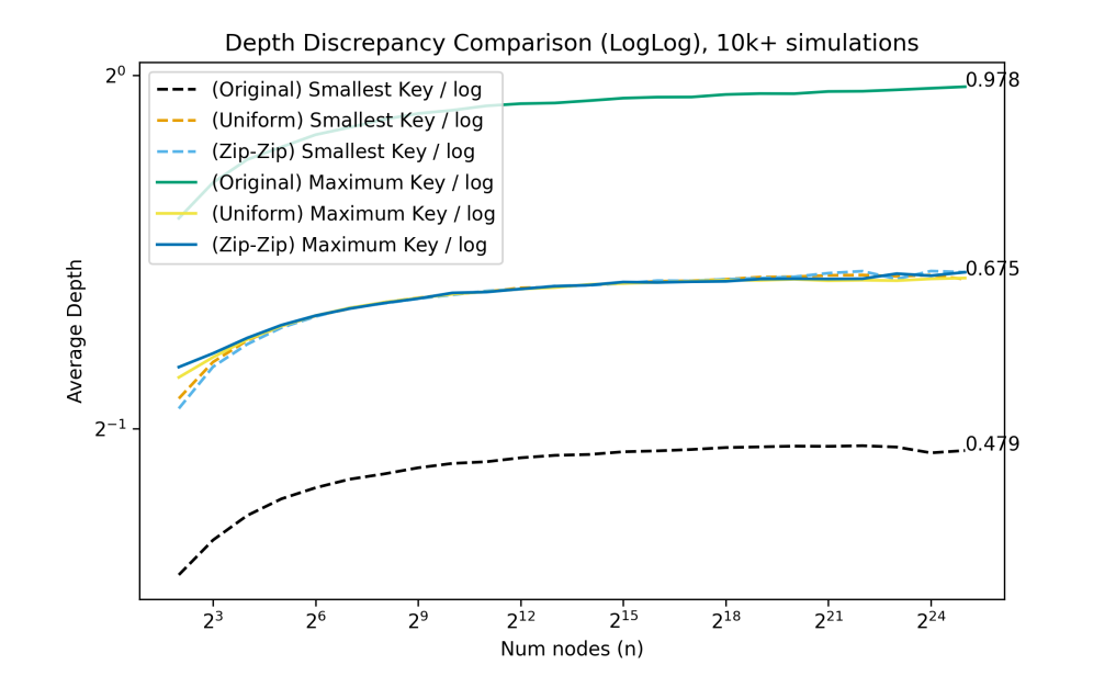
Figure 4: Experimental results for the depth discrepancy between the smallest and largest keys in the original, uniform (treap), and zip-zip variants of the zip tree. Each data point is scaled down by a factor of $\log n$ (base 2).

4.1 Depth Discrepancy

First, we consider the respective depths of the smallest and the largest keys in an original zip tree, compared with the depths of these keys in a zip-zip tree. See Figure 4. The empirical results for the depths for smallest and largest keys in a zip tree clearly match the theoretic expected values of 0.5 $\log n$ and $\log n$, respectively, from Theorem 2.2. For comparison purposes, we also plot the depths for smallest and largest keys in a uniform zip tree, which is essentially a treap, and in a zip-zip tree (with static $r_{2}$-ranks). Observe that, after the number of nodes, $n$, grows beyond small tree sizes, there is no discernible difference between the depths of the largest and smallest keys, and that this is very close to the theoretical bound of $0.69\log n$. Most notably, apart from some differences for very small trees, the depths for smallest and largest keys in a zip-zip tree quickly conform to the uniform zip tree results, while using exponentially fewer bits for each node’s rank.

4.2 Average Key Depth and Tree Height

Next, we empirically study the average key depth and average height for the three aforementioned zip tree variants. See Figure 5. Notably, we observe that for all tree sizes, despite using exponentially fewer rank bits per node, the zip-zip tree performs indistinguishably well from the uniform zip tree, equally outperforming the original zip tree variant. The average key depths and average tree heights for all variants appear to approach some constant multiple of $\log n$. For example, the average depth of a key in an original zip tree, uniform zip tree, and zip-zip tree reached $1.373\log n$, $1.267\log n$, $1.267\log n$, respectively. Interestingly, these values are roughly 8.5% less than the original zip tree and treap theoretical average key depths of $1.5\log n$ [27] and $1.39\log n$ [24], respectively, suggesting that both variants approach their limits at a similar rate. Also, we note that our empirical average height bounds for uniform zip trees and zip-zip trees get as high as $2.542\log n$. It is an open problem to bound these expectations theoretically, but we show in an appendix that the height of a zip-zip tree is at most $3.82\log n$ with probability $1-o(1)$, which clearly beats the $4.31107\log n$ expected height for a randomly-constructed binary search tree [8, 9, 12, 22].

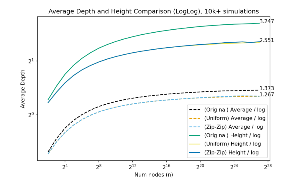
Figure 5: Experimental results for the average node depth and tree height, comparing the original, uniform (treap-like), and zip-zip variants of the zip tree. Each data point is scaled down by a factor of $\log n$ (base 2).

4.3 Rank Comparisons

Next, we experimentally determine the frequency of complete rank ties (collisions) for the uniform and zip-zip variants. See Figure 6 (left). The experiments show how the frequencies of rank collisions decrease polynomially in $n$ for the uniform zip tree and in $\log n$ for the second rank of the zip-zip variant. This reflects how these rank values were drawn uniformly from a range of $n^{c}$ and $\log^{c}n$, respectively. Specifically, we observe the decrease to be polynomial to $n^{-2.97}$ and $\log^{-2.99}{n}$, matching our chosen value of $c$ being 3.

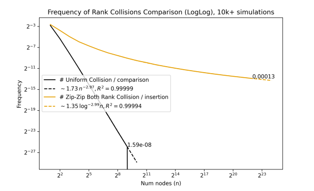
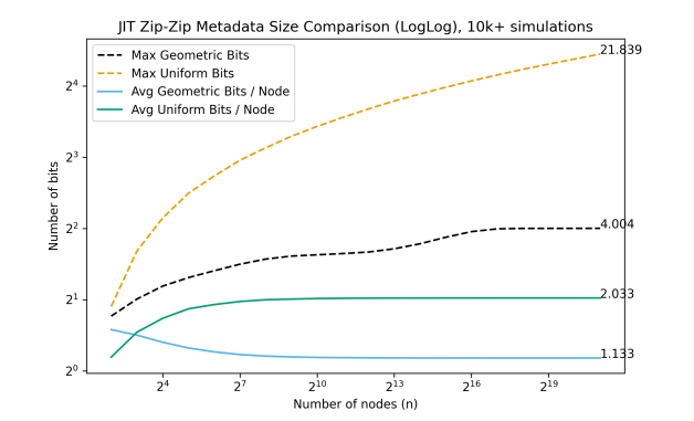
Figure 6: (Left) The frequency of encountered rank ties per rank comparison for the uniform variant and per element insertion for the zip-zip variant. (Right) The metadata size for the just-in-time implementation of the zip-zip tree.

4.4 Just-in-Time Zip-zip Trees

Finally, we show how the just-in-time zip-zip tree variant uses an expected constant number of bits per node. See Figure 6 (right). We observe a results of only $1.133$ bits per node for storing the geometric ($r_{1}$) rank differences, and only $2.033$ bits per node for storing the uniform ($r_{2}$) ranks, leading to a remarkable total of $3.166$ expected bits per node of rank metadata to achieve ideal treap properties.

5 Biased Zip-zip Trees

In this section, we describe how to make zip-zip trees biased for weighted keys. In this case, we assume each key, $k$, has an associated weight, $w_{k}$, such as an access frequency. Without loss of generality, we assume that weights don’t change, since we can simulate a weight change by deleting and reinserting a key with its new weight.

Our method for modifying zip-zip trees to accommodate weighted keys is simple—when we insert a key, $k$, with weight, $w_{k}$, we now assign $k$ a rank pair, $r=(r_{1},r_{2})$, such that $r_{1}$ is $\lfloor\log w_{k}\rfloor+X_{k}$, where $X_{k}$ is drawn independently from a geometric distribution with success probability $1/2$, and $r_{2}$ is an integer independently chosen uniformly in the range from $1$ to $\lceil\log^{c}n\rceil$, where $c\geq 3$. Thus, the only modification to our zip-zip tree construction to define a biased zip-zip tree is that the $r_{1}$ component is now a sum of a logarithmic rank and a value drawn from a geometric distribution. As with our zip-zip tree definition for unweighted keys, all the update and search operations for biased zip-zip trees are the same as for the original zip trees, except for this modification to the rank, $r$, for each key (and performing rank comparisons lexicographically). Therefore, assuming polynomial weights, we still can represent each such rank, $r$, using $O(\log\log n)$ bits w.h.p.

We also have the following theorem, which implies the expected search performance bounds for weighted keys.

Theorem 5.1

The expected depth of a key, $k$, with weight, $w_{k}$, in a biased zip-zip tree storing a set, $\mathcal{K}$, of $n$ keys is $O(\log(W/w_{k}))$, where $W=\sum_{k\in\mathcal{K}}w_{k}$.

Proof

By construction, a biased zip-zip tree, $T$, is dual to a biased skip list, $L$, defined on $\mathcal{K}$ with the same $r_{1}$ ranks as for the keys in $\mathcal{K}$ as assigned during their insertions into $T$. Bagchi, Buchsbaum, and Goodrich [4] show that the expected depth of a key, $k$, in $L$ is $O(\log(W/w_{k}))$. Therefore, by Theorem 2.1, and the linearity of expectation, the expected depth of $k$ in $T$ is $O(\log(W/w_{k}))$, where, as mentioned above, $W$ is the sum of the weights of the keys in $T$ and $w_{k}$ is the weight of the key, $k$. ∎

Thus, a biased zip-zip tree has similar expected search and update performance as a biased skip list, but with reduced space, since a biased zip-zip tree has exactly $n$ nodes, whereas, assuming a standard skip-list representation where we use a linked-list node for each instance of a key, $k$, on a level in the skip list (from level-0 to the highest level where $k$ appears) a biased skip list has an expected number of nodes equal to $2n+2\sum_{k\in\mathcal{K}}\log w_{k}$. For example, if there are $n^{\varepsilon}$ keys with weight $n^{\varepsilon}$, then such a biased skip list would require $\Omega(n\log n)$ nodes, whereas a dual biased zip-zip tree would have just $n$ nodes.

Further, due to their simplicity and weight biasing, we can utilize biased zip-zip trees as the biased auxiliary data structures in the link-cut dynamic tree data structure of Sleator and Tarjan [26], thereby providing a simple implementation of link-cut trees.

Appendix 0.A Insertion and Deletion in Zip Trees and Zip-zip Trees

The insertion and deletion algorithms for zip-zip trees are the same as those for zip trees, except that in a zip-zip tree tree a node’s rank is a pair $(r_{1},r_{2})$, as we explain above, and rank comparisons are done lexicographically on these pairs.

To insert a new node $x$ into a zip tree, we search for $x$ in the tree until reaching the node $y$ that $x$ will replace, namely the node $y$ such that $y.rank\leq x.rank$, with strict inequality if $y.key<x.key$. From $y$, we follow the rest of the search path for $x$, unzipping it by splitting it into a path, $P$, containing each node with key less than $x.key$ and a path, $Q$, containing each node with key greater than $x.key$ (recall that we assume keys are distinct) [27]. To delete a node $x$, we perform the inverse operation, where we do a search to find $x$ and let $P$ and $Q$ be the right spine of the left subtree of $x$ and the left spine of the right subtree of $x$, respectively. Then we zip $P$ and $Q$ to form a single path $R$ by merging them from top to bottom in non-increasing rank order, breaking a tie in favor of the smaller key [27]. See Figure 7.

Figure 7: How insertion in a zip tree is done via unzipping and deletion is done via zipping.

For completeness, we give the pseudo-code for the insert and delete operations, from Tarjan, Levy, and Timmel [27], in Figures 8 and 9.

Insert$x$

$rank\leftarrow x.rank\leftarrow$ RandomRank

$key\leftarrow x.key$

$cur\leftarrow root$ $cur\neq\text{null}$ and $(rank<cur.rank$ or $(rank=cur.rank$ and $key>cur.key))$

$prev\leftarrow cur$

$cur\leftarrow\textbf{if}~{}key<cur.key~{}\textbf{then}~{}cur.left~{}\textbf{else}~{}cur.right$

$\textbf{if}~{}cur=root~{}\textbf{then}~{}root\leftarrow x$

$\textbf{else if}~{}key<prev.key~{}\textbf{then}~{}prev.left\leftarrow x$

$\textbf{else}~{}prev.right\leftarrow x$

$\textbf{if}~{}cur=\text{null}~{}\textbf{then}~{}\{~{}x.left\leftarrow x.right\leftarrow\text{null};~{}\Return~{}\}$

$\textbf{if}~{}key<cur.key~{}\textbf{then}~{}x.right\leftarrow cur~{}\textbf{else}~{}x.left\leftarrow cur$

$prev\leftarrow x$

$cur\neq\text{null}$

$fix\leftarrow prev$

$cur.key<key$ $~{}\{~{}prev\leftarrow cur;~{}cur\leftarrow cur.right~{}\}$ $cur=\text{null}$ or $cur.key<key$ $~{}\{~{}prev\leftarrow cur;~{}cur\leftarrow cur.left~{}\}$ $cur=\text{null}$ or $cur.key>key$ $fix.key>key$ or $(fix=x$ and $prev.key>key)$

$fix.left\leftarrow cur$

$fix.right\leftarrow cur$

Figure 8: Insertion in a zip tree (or zip-zip tree), from [27].

Delete$x$

$key\leftarrow x.key$

$cur\leftarrow root$ $key\neq cur.key$

$prev\leftarrow cur$

$cur\leftarrow\textbf{if}~{}key<cur.key~{}\textbf{then}~{}cur.left~{}\textbf{else}~{}cur.right$

$left\leftarrow cur.left;~{}right\leftarrow cur.right$

$\textbf{if}~{}left=\text{null}~{}\textbf{then}~{}cur\leftarrow right$

$\textbf{else if}~{}right=\text{null}~{}\textbf{then}~{}cur\leftarrow left$

$\textbf{else if}~{}left.rank\geq right.rank~{}\textbf{then}~{}cur\leftarrow left$

$\textbf{else}~{}cur\leftarrow right$

$\textbf{if}~{}root=x~{}\textbf{then}~{}root\leftarrow cur$

$\textbf{else if}~{}key<prev.key~{}\textbf{then}~{}prev.left\leftarrow cur$

$\textbf{else}~{}prev.right\leftarrow cur$

$left\neq\text{null}$ and $right\neq\text{null}$ $left.rank\geq right.rank$ $~{}\{~{}prev\leftarrow left;~{}left\leftarrow left.right~{}\}$ $left=\text{null}$ or $left.rank<right.rank$

$prev.right\leftarrow right$ $~{}\{~{}prev\leftarrow right;~{}right\leftarrow right.left~{}\}$ $right=\text{null}$ or $left.rank\geq right.rank$

$prev.left\leftarrow left$

Figure 9: Deletion in a zip tree (or zip-zip tree), from [27].

Appendix 0.B Omitted Proofs

In this appendix, we provide proofs that were omitted in the body of this paper. We start with a simple lemma that our omitted proofs use.

Lemma 3

Let $X$ be the sum of $n$ independent geometric random variables with success probability $1/2$. Then, for $t\geq 2$,

$$\Pr(X>(2+t)n)\leq e^{-tn/10}.$$

Proof

The proof follows immediately by a Chernoff bound for a sum of $n$ independent geometric random variables (see, e.g., Goodrich and Tamassia [13, pp. 555–556]). ∎

0.B.1 Compacting a JIT Zip-zip Tree

We prove the following theorem in this appendix.

Theorem 0.B.1 (Same as Theorem 3.1)

Let $T$ be a JIT zip-zip tree resulting from $n$ update operations starting from an initially-empty tree. The expected number of bits for rank metadata in any non-root node in $T$ is $O(1)$ and the number of bits required for all the rank metadata in $T$ is $O(n)$ w.h.p.

Proof

By the duality between zip trees and skip lists, the set of nodes in an $r_{1}$-rank group in $T$ is dual to a sequence, $L$, of consecutive nodes in a level-$r_{1}$ list in the skip list but not in the level-$(r_{1}+1)$ list. Thus, since $v$ is not the root, there is a node, $u$, that is the immediate predecessor of the first node in $L$ in the level-$r_{1}$ list in the skip list, and there is a node, $w$, that is the immediate successor of the last node in $L$ in the level-$r_{1}$ list in the skip list. Moreover, both $u$ and $v$ are in the level-$(r_{1}+1)$ list in the skip list, and (since $v$ is not the root) it cannot be the case that $u$ stores the key $-\infty$ and $w$ stores the key $+\infty$. As an over-estimate and to avoid dealing with dependencies, we will consider the $r_{1}$-rank differences determined by predecessor nodes (like $u$) separate from the $r_{1}$-rank differences determined by successor nodes (like $w$). Let us focus on predecessors, $u$, and suppose $u$ does not store $-\infty$. Let $r_{1}^{\prime}>r_{1}$ be the highest level in the skip list where $u$ appears. Then the difference between the $r_{1}$-rank of $v$ and its parent is at most $r_{1}^{\prime}-r_{1}$. That is, this rank difference is at most a random variable that is drawn from a geometric distribution with success probability $1/2$ (starting at level $r_{1}+1$); hence, its expected value is at most $2$. Further, for similar reasons, the sum of all the $r_{1}$-rank differences for all nodes in $T$ that are determined because of a predecessor node (like $u$) can be bounded by the sum, $X$, of $n$ independent geometric random variables with success probability $1/2$. (Indeed, this is also an over-estimate, since a $r_{1}$-rank difference for a parent in the same $r_{1}$-rank group is 0, and some $r_{1}$-rank differences may be determined by a successor node that has a lower highest level in the dual skip list that a predecessor node.) By Lemma 3, $X$ is $O(n)$ with (very) high probability, and a similar argument applies to the sum of $r_{1}$-rank differences determined by successor nodes. Thus, with (very) high probability, the sum of all $r_{1}$-rank differences between children and parents in $T$ is $O(n)$.

Let us next consider all the $r_{2}$-ranks in a JIT zip-zip tree. Recall that each time there is a rank tie when using existing $(r_{1},r_{2})$ ranks, during a given update, we augment the two $r_{2}$ ranks bit by bit until they are different. That is, the length of each such augmentation is a geometric random variable with success probability $1/2$. Further, by the way that the zip and unzip operations work, the number of such encounters that could possibly have a rank tie is upper bounded by the sum of the $r_{1}$-ranks of the keys involved, i.e., by the sum of $n$ geometric random variables with success probability $1/2$. Thus, by Lemma 3, the number of such encounters is at most $N=12n$ and the number of added bits that occur during these encounters is at most $12N$, with (very) high probability. ∎

0.B.2 Partially-Persistent Zip-zip Trees

We show in this appendix that one can efficiently make a zip-zip tree partially persistent.

Theorem 0.B.2 (Same as Theorem 3.3)

One can transform an initially-empty zip-zip tree, $T$, to be partially persistent, over the course of $n$ insert and delete operations, so as to support, w.h.p., $O(\log n)$ amortized-time updates in the current version and $O(\log n)$-time queries in the current or past versions, using $O(n)$ space.

Proof

By the way that the zip and unzip operations work, the total number of data or pointer changes in $T$ over the course of $n$ insert and delete operations can be upper bounded by the sum of $r_{1}$-ranks for all the keys involved, i.e., by the sum of $n$ geometric random variables with success probability $1/2$. Thus, by Lemma 3, the number of data or pointer changes in $T$ is at most $N=12n$ with (very) high probability. Driscoll, Sarnak, Sleator, and Tarjan [10] show how to make any bounded-degree linked structure, like a binary search tree, $T$, into a partially persistent data structure by utilizing techniques employing “fat nodes” and “node splitting,” so that if a sequence of $n$ updates on $T$ only modifies $O(n)$ data fields and pointers, then $T$ can be made partially persistent with only an constant-factor increase in time and space for processing the sequence of updates, and this allows for queries in any past instance of $T$ in the same asymptotic time as in the ephemeral version of $T$ plus the time to locate the appropriate prior version. Alternatively, Sarnak and Tarjan [23] provide a simpler set of techniques that apply to binary search trees without parent parent pointers. Combining these facts establishes the theorem. ∎

For example, we can apply this theorem with respect to a sequence of $n$ updates of a zip-zip tree that can be performed in $O(n\log n)$ time and $O(n)$ space w.h.p., e.g., to provide a simple construction of an $O(n)$-space planar point-location data structure that supports $O(\log n)$-time queries. A similar construction was provided by Sarnak and Tarjan [23], based on the more-complicated red-black tree data structure; hence, our construction can be viewed as simplifying their construction.

Theorem 0.B.3

The height of a zip-zip tree, $T$, holding a set, $S$, of $n$ keys is at most $3.82\log n$ with probability $1-o(1)$.

Proof

As in the proof of Theorem 3.2, we note that the depth, $X$, in $T$ of the $i$-th smallest key, $x_{i}$, can be characterized as follows. Let

$$L_{i}=\sum_{1\leq j<i}X_{j},\mbox{~{}~{}~{}~{}and~{}~{}~{}~{}}R_{i}=\sum_{i<j\leq n}X_{j},$$

where $X_{j}$ is a 0-1 random variable that is 1 if and only if $x_{j}$ is an ancestor of $x_{i}$, where $x_{i}$ is the $i$-th smallest key in $S$ and $x_{j}$ is the $j$-th smallest key. Then $X=1+L_{i}+R_{i}$. Further, note that the random variables that are summed in $L_{i}$ (or, respectively, $R_{i}$) are independent, and, focusing on $E[X|C]$, as in the proof of Theorem 3.2, $E[L_{i}]=H_{i}-1$ and $E[R_{i}]=H_{n-i+1}-1$, where $H_{m}=\sum_{k=1}^{m}1/k$ is the $m$-th Harmonic number; hence, $E[X|C]=H_{i}+H_{n-i+1}-1<2\ln n-1$. Thus, we can apply a Chernoff bound to characterize $X$ by bounding $L_{i}$ and $R_{i}$ separately (w.l.o.g., we focus on $L_{i}$), conditioned on $C$ holding. For example, for the high-probability bound for the proof, it is sufficient that, for some small constant, $\varepsilon>0$, there is a reasonably small $\delta>0$ such that

$$P(L_{i}>(1+\delta)\ln n)<2^{-((1+\varepsilon)/\ln 2)(\ln 2)\log n}=2^{-(1+\varepsilon)\log n}=1/n^{1+\varepsilon},$$

which would establish the theorem by a union bound. In particular, we choose $\delta=1.75$ and let $\mu=E[L_{i}]$. Then by a Chernoff bound, e.g., see [3, 15, 18, 19, 25], for $\mu=\ln n$, we have the following:

$$\Pr(L_{i}>2.75\ln n) = \Pr(L_{i}>(1+\delta)\mu)$$

$$< \left({\frac{e^{\delta}}{(1+\delta)^{1+\delta}}}\right)^{\mu}$$

$$= \left({\frac{e^{1.75}}{2.75^{2.75}}}\right)^{\ln n}$$

$$\leq 2.8^{-(\ln 2)\log n}$$

$$\leq 2.04^{-\log n}$$

$$= \frac{1}{n^{\log 2.04}},$$

which establishes the above bound for $\varepsilon=\log_{2}2.04-1>0$. Combining this with a similar bound for $R_{i}$, and the derived from Markov’s inequality with respect to $E[X|A]$ and $E[X|B]$, given in the proof of Theorem 3.2 for the conditional events $A$ and $B$, we get that the height of of a zip-zip tree is at most

$$2(2.75)(\ln 2)\log n\leq 3.82\log n,$$

with probability $1-o(1)$. ∎

References

- [1] Acar, U.A.: Self-Adjusting Computation. Ph.D. thesis, Carnegie Mellon Univ. (2005)
- [2] Afek, Y., Kaplan, H., Korenfeld, B., Morrison, A., Tarjan, R.E.: The CB tree: a practical concurrent self-adjusting search tree 27(6), 393–417. https://doi.org/10.1007/s00446-014-0229-0, https://doi.org/10.1007/s00446-014-0229-0
- [3] Alon, N., Spencer, J.H.: The Probabilistic Method. John Wiley & Sons, 4th edn. (2016)
- [4] Bagchi, A., Buchsbaum, A.L., Goodrich, M.T.: Biased skip lists. Algorithmica 42, 31–48 (2005)
- [5] Bender, M.A., Conway, A., Farach-Colton, M., Kuszmaul, W., Tagliavini, G.: Tiny pointers. In: ACM-SIAM Symposium on Discrete Algorithms (SODA). pp. 477–508 (2023). https://doi.org/10.1137/1.9781611977554.ch21, https://epubs.siam.org/doi/abs/10.1137/1.9781611977554.ch21
- [6] Bent, S.W., Sleator, D.D., Tarjan, R.E.: Biased search trees. SIAM Journal on Computing 14(3), 545–568 (1985)
- [7] Dean, B.C., Jones, Z.H.: Exploring the duality between skip lists and binary search trees. In: Proc. of the 45th Annual Southeast Regional Conference (ACM-SE). pp. 395–399 (2007). https://doi.org/10.1145/1233341.1233413, https://doi.org/10.1145/1233341.1233413
- [8] Devroye, L.: A note on the height of binary search trees. J. ACM 33(3), 489–498 (1986)
- [9] Devroye, L.: Branching processes in the analysis of the heights of trees. Acta Informatica 24(3), 277–298 (1987)
- [10] Driscoll, J.R., Sarnak, N., Sleator, D.D., Tarjan, R.E.: Making data structures persistent. Journal of Computer and System Sciences 38(1), 86–124 (1989). https://doi.org/https://doi.org/10.1016/0022-0000(89)90034-2, https://www.sciencedirect.com/science/article/pii/0022000089900342
- [11] Eberl, M., Haslbeck, M.W., Nipkow, T.: Verified analysis of random binary tree structures. In: 9th Int. Conf. on Interactive Theorem Proving (ITP). pp. 196–214. Springer (2018)
- [12] Flajolet, P., Odlyzko, A.: The average height of binary trees and other simple trees. Journal of Computer and System Sciences 25(2), 171–213 (1982)
- [13] Goodrich, M.T., Tamassia, R.: Algorithm Design and Applications. Wiley (2015)
- [14] Guo, B.N., Qi, F.: Sharp bounds for harmonic numbers. Applied Mathematics and Computation 218(3), 991–995 (2011). https://doi.org/https://doi.org/10.1016/j.amc.2011.01.089, https://www.sciencedirect.com/science/article/pii/S009630031100124X
- [15] Hagerup, T., Rüb, C.: A guided tour of Chernoff bounds. Information Processing Letters 33(6), 305–308 (1990)
- [16] Hartline, J.D., Hong, E.S., Mohr, A.E., Pentney, W.R., Rocke, E.C.: Characterizing history independent data structures. Algorithmica 42, 57–74 (2005)
- [17] Martínez, C., Roura, S.: Randomized binary search trees. J. ACM 45(2), 288–323 (1998). https://doi.org/10.1145/274787.274812, https://doi.org/10.1145/274787.274812
- [18] Mitzenmacher, M., Upfal, E.: Probability and Computing: Randomization and Probabilistic Techniques in Algorithms and Data Analysis. Cambridge University Press, 2nd edn. (2017)
- [19] Motwani, R., Raghavan, P.: Randomized Algorithms. Cambridge University Press (1995)
- [20] Papadakis, T., Ian Munro, J., Poblete, P.V.: Average search and update costs in skip lists. BIT Numerical Mathematics 32(2), 316–332 (1992)
- [21] Pugh, W.: Skip lists: A probabilistic alternative to balanced trees. Commun. ACM 33(6), 668–676 (jun 1990). https://doi.org/10.1145/78973.78977, https://doi.org/10.1145/78973.78977
- [22] Reed, B.: The height of a random binary search tree. J. ACM 50(3), 306–332 (2003)
- [23] Sarnak, N., Tarjan, R.E.: Planar point location using persistent search trees. Communications of the ACM 29(7), 669–679 (1986)
- [24] Seidel, R., Aragon, C.R.: Randomized search trees. Algorithmica 16(4-5), 464–497 (1996)
- [25] Shiu, D.: Efficient computation of tight approximations to Chernoff bounds. Computational Statistics pp. 1–15 (2022)
- [26] Sleator, D.D., Tarjan, R.E.: A data structure for dynamic trees. In: 13th ACM Symposium on Theory of Computing (STOC). pp. 114–122 (1981)
- [27] Tarjan, R.E., Levy, C., Timmel, S.: Zip trees. ACM Trans. Algorithms 17(4), 34:1–34:12 (2021). https://doi.org/10.1145/3476830, https://doi.org/10.1145/3476830