Machine learning for option pricing:∑an empirical investigation of network architectures

Abstract.

We consider the supervised learning problem of learning the price of an option or the implied volatility given appropriate input data (model parameters) and corresponding output data (option prices or implied volatilities). The majority of articles in this literature considers a (plain) feed forward neural network architecture in order to connect the neurons used for learning the function mapping inputs to outputs. In this article, motivated by methods in image classification and recent advances in machine learning methods for PDEs, we investigate empirically whether and how the choice of network architecture affects the accuracy and training time of a machine learning algorithm. We find that for option pricing problems, where we focus on the Black–Scholes and the Heston model, the generalized highway network architecture outperforms all other variants, when considering the mean squared error and the training time as criteria. Moreover, for the computation of the implied volatility, after a necessary transformation, a variant of the DGM architecture outperforms all other variants, when considering again the mean squared error and the training time as criteria.

1. Introduction

Machine learning has taken the field of mathematical finance by a storm, and there are numerous applications of machine learning in finance by now. Concrete applications include, for example, the computation of option prices and implied volatilities as well as the calibration of financial models, see e.g. Liu et al. [30], Horvath et al. [28], Cuchiero et al. [12], approaches to hedging, see e.g. Buehler et al. [10], portfolio selection and optimization, see e.g. Pinelis and Ruppert [34], Zhang et al. [41], risk management, see e.g. Boudabsa and Filipović [9], Fernandez-Arjona and Filipović [19], Eckstein et al. [16], optimal stopping problems, see e.g. Bayer et al. [5, 4], Becker et al. [7, 6], model-free and robust finance, see e.g. Eckstein and Kupper [15], Neufeld and Sester [32], Eckstein et al. [17], stochastic games and optimal control problems, see e.g. Huré et al. [29], Bachouch et al. [3], as well as the solution of high-dimensional PDEs, see e.g. Sirignano and Spiliopoulos [37], Han et al. [24], Georgoulis et al. [22]. A comprehensive overview of applications of machine learning in mathematical finance appears in the recent volume of Capponi and Lehalle [11], while an exhaustive overview focusing on pricing and hedging appears in Ruf and Wang [35].

We are interested in the computation of option prices and implied volatilities using machine learning methods, and thus, implicitly, in model calibration as well. More specifically, we consider the supervised learning problem of learning the price of an option or the implied volatility given appropriate input data (model parameters) and corresponding output data (option prices or implied volatilities). The majority of articles in this literature, see e.g. Horvath et al. [28], Cuchiero et al. [12], Liu et al. [30], consider a (plain) feed forward neural network architecture in order to connect the neurons used for learning the function mapping inputs to outputs. In this article, motivated by methods in image classification, see e.g. He et al. [25], Srivastava et al. [39], He et al. [26], and recent advances in machine learning methods for PDEs, see e.g. Sirignano and Spiliopoulos [37], we investigate empirically whether and how the choice of network architecture affects the speed of a machine learning algorithm, and we are interested in the “optimal” network architecture for these problems.

More specifically, next to the classical feed forward neural network or multilayer perceptron (MLP) architecture, we consider residual neural networks, highway networks and generalized highway networks. These network architectures have been successfully applied in image classification problems, see e.g. He et al. [26]. Moreover, motivated by the recent work of Sirignano and Spiliopoulos [38] on the deep Galerkin method (DGM) for solving high-dimensional PDEs, we also consider the DGM network architecture, and, in addition, we construct and test two variants of this architecture.

The empirical results show that the more advanced network architectures consistently outperform the MLP architecture, and should thus be preferred for the computation of option prices and implied volatilities. More specifically, we find that for option pricing problems, where we focus on the Black–Scholes and the Heston model, the generalized highway network architecture outperforms all other variants, when considering the mean squared error and the computational time as criteria. Moreover, we find that for the computation of the implied volatility, after a necessary transformation, a variant of the DGM architecture outperforms all other variants, when considering again the mean squared error and the computational time as criteria.

The remainder of this paper is organized as follows: in Section 2 we briefly introduce the models used in this article, and in Section 3 we outline the basics of neural networks. In Section 4 we describe the different network architectures that will be used throughout, namely residual networks, highway and generalized highway networks, as well as the DGM network and its two variants. In Section 5 we revisit the main problems and describe the method used for generating sample data. In Section 6 we present the results of the empirical analysis performed, where the different network architectures are compared, with main criteria being accuracy and computational time. Finally, Section 7 contains a synopsis and some concluding remarks from the empirical analysis.

2. Models

In this brief section, we are going to review the models we will use for option pricing and recall the definition of implied volatility, in order to fix the notation for the remainder of this work.

Let $(\Omega,\mathcal{F},\mathbb{F},\mathbb{Q})$ denote a complete stochastic basis, where $\mathbb{F}=(\mathcal{F}_{t})_{t\in[0,T]}$ is the filtration, $T>0$ is a fixed and finite time horizon, while $\mathbb{Q}$ denotes an equivalent martingale measure for an asset $S$ with price process $S=(S_{t})_{t\in[0,T]}$, adapted to the filtration $\mathbb{F}$.

We will first consider the Black and Scholes [8] model for the evolution of the asset price $S$, i.e.

$$\mathrm{d}S_{t}=rS_{t}\mathrm{d}t+\sigma S_{t}\mathrm{d}W_{t},\quad S_{0}>0,$$ (2.1)

where $r$ denotes the risk-free interest rate, $\sigma$ the volatility and $W$ denotes a $\mathbb{Q}$-Brownian motion. The price of a European call option with payoff $C=(S_{T}-K)^{+}$ in this model is provided by the celebrated Black–Scholes formula, i.e.

$$\begin{split}\pi_{t}(C;K,T,\sigma)&=S_{t}\Phi(d_{1})-\mathrm{e}^{-r(T-t)}K\Phi(d_{2}),\\ d_{1}&=\frac{\log\big{(}\frac{S_{t}}{K}\big{)}+(r+\frac{1}{2}\sigma^{2})(T-t)}{\sigma\sqrt{T-t}}=d_{2}+\sigma\sqrt{T-t},\end{split}$$ (2.2)

where $\Phi(\cdot)$ denotes the cumulative distribution function (cdf) of the standard normal distribution.

Assume that we can observe in a financial market the traded prices $\pi_{t}^{\mathrm{M}}(C;K,T)$ for a call option $C$, for various strikes $K$ and maturities $T$. The implied volatility $\sigma_{\mathrm{iv}}(K,T)$ is the volatility that should be inserted into the Black–Scholes equation (2.2) such that the model price $\pi_{t}(C;K,T,\sigma)$ matches the traded market price $\pi_{t}^{\mathrm{M}}(C;K,T)$, i.e.

$$\pi_{t}(C;K,T,\sigma_{\mathrm{iv}}(K,T))=\pi_{t}^{\mathrm{M}}(C;K,T),$$ (2.3)

see e.g. Gatheral [21, Ch. 1]. The inverse problem in (2.3) does not admit a closed form solution and needs to be solved numerically, using methods such as the Newton–Raphson or Brent; see e.g. Liu et al. [30] for more details. The Black–Scholes model assumes that the volatility is constant, however the implied volatility computed from real market option prices exhibits a so-called smile or skew shape; see e.g. Figure 2.1 for a visualization.

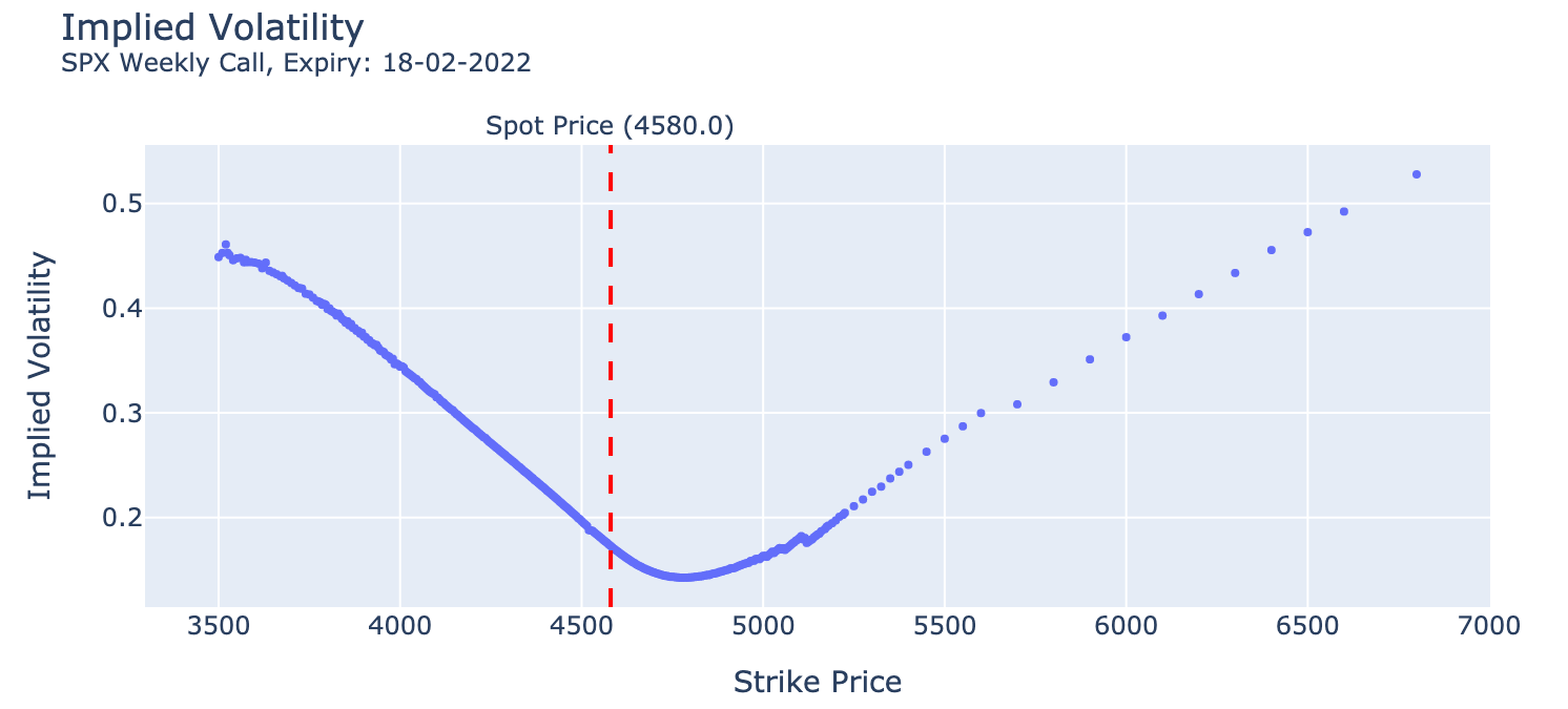
Figure 2.1. The market implied volatility for CBOE’s SPX options.

A popular model that captures the behavior of market data is the Heston stochastic volatility model, cf. Heston [27]. The dynamics of the asset price in this model are provided by the following SDEs

$$\begin{cases}\mathrm{d}S_{t}=rS_{t}\mathrm{d}t+\sqrt{v_{t}}S_{t}\mathrm{d}W_{t},&S_{0}>0\\ \mathrm{d}v_{t}=\kappa(\theta-v_{t})\mathrm{d}t+\eta\sqrt{v_{t}}\mathrm{d}\widetilde{W}_{t},&v_{0}>0,\end{cases}$$ (2.4)

where $\kappa,\theta,\eta$ denote positive constants and $[W,\widetilde{W}]=\rho$ denotes the correlation between the two $\mathbb{Q}$-Brownian motions. The tuple of the log-asset price process and the volatility process $(\log S,v)$ is an affine process, see e.g. Filipović [20, Ch. 10], and the characteristic function of the log-asset price can be computed explicitly. Therefore, option prices in the Heston model can be computed efficiently using Fourier transform methods, see e.g. Eberlein et al. [14], or the COS method of Fang and Oosterlee [18].

3. Fundamentals of neural networks

In this section, we will briefly discuss the components that embody a neural network in order to fix the relevant notation, and also present the simplest network architecture, the multilayer perceptron.

A perceptron is a function that takes an input $\mathbf{x}\in\mathbb{R}^{d}$, performs an operation on it, and outputs $\mathbf{y}\in\mathbb{R}^{e}$ ($d\neq e$ in general). The operation is typically the multiplication of $\mathbf{x}$ with a weight vector $\mathbf{w}$, the addition of a bias factor $b$ and the application of an activation function $H$, i.e.

$$\mathbf{y}=H\left(\sum_{i=1}^{d}w_{i}x_{i}+b\right)=H\left(\mathbf{w}\cdot\mathbf{x}+b\right).$$ (3.1)

Here $\cdot$ denotes the usual inner product between two vectors, or the multiplication of a vector and a matrix.

The activation function $H$ is typically a non-linear function, such that the output cannot be reproduced from a linear combination of inputs, and also differentiable, such that the stochastic gradient descent algorithm can be applied for computing the weights and bias parameters. Typical examples of activation functions are the following:

• The sigmoid function, where $H_{\rm sig}(x)=\frac{1}{1+\mathrm{e}^{-x}}$.

• The hyperbolic tangent function, where $H_{\rm tanh}(x)=\frac{\mathrm{e}^{x}-\mathrm{e}^{-x}}{\mathrm{e}^{x}+\mathrm{e}^{-x}}$.

• The Rectified Linear Unit (ReLU), where $H_{\rm ReLU}(x)=\max\{0,x\}$.

• The Gaussian Error Linear Unit (GELU), where $H_{\rm GELU}(x)=x\Phi(x)$, with $\Phi$ the normal cdf.

• The softmax function, where $H_{\rm sm}(\mathbf{x})_{i}=\frac{\mathrm{e}^{x_{i}}}{\sum_{j=1}^{K}\mathrm{e}^{x_{j}}}$.

A layer is a stack of perceptrons which generally all depend on the same previous input. This input could be either the input data or the output from a previous layer. Then, we can have many perceptrons in one layer being connected to many perceptrons in the subsequent layer. Assume that the first layer has $m$ perceptrons, and the second layer has $n$. We denote the connection between perceptron $i$ and $j$ as $W_{ij}$, where $W$ is an $m\times n$ matrix. If such a connection exists, the value $W_{ij}$ is the weight that perceptron $i$ contributes to the input of perceptron $j$. If there is no connection between $i$ and $j$, then $W_{ij}=0$. Using the weight matrix $W$ and the bias vector $\mathbf{b}$, we can update (3.1) as follows

$$y_{i}=H_{i}\left(\sum_{j=1}^{n}W_{ij}x_{j}+b_{j}\right),$$ (3.2)

where $H_{i}$ is the activation function and $y_{i}$ the output of perceptron $i$. We generally use the same activation function for each perceptron in a layer, in which case $H_{j}=H_{i}$ for all $i,j\in\{1,\dots,n\}$.

The simplest example of a neural network is illustrated in Figure 3.1, where the layers are densely connected, i.e. the outputs of one layer are the inputs for all perceptrons in the next layer. This network is called a multilayer perceptron (MLP).

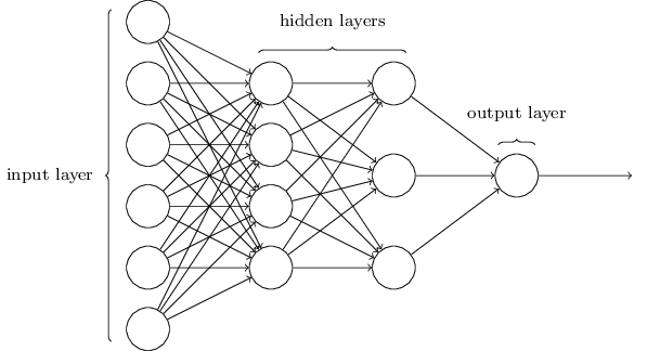
Figure 3.1. A visual representation of a multilayer perceptron.

In order to compute a desired quantity using a neural network, we need to estimate the appropriate parameters for the layers (perceptrons) of the network. Using the distance between the network output and the target output as an error measure, we can update the weights and biases in order to minimize this error. We refer to this distance as the loss, and call the function we minimize the loss function $J$, hence

$$J(\theta):=\|H(\mathbf{x};\theta)-\mathbf{y}\|,$$ (3.3)

where $\mathbf{y}$ is the target output and $H(\mathbf{x};\theta)$ is the actual output of the network given the input $\mathbf{x}$ and the parameters $\theta$. We will apply the stochastic gradient descent (SGD) algorithm in order to estimate the parameters of the network. The SGD is based on the following iterative updating formula for the computation of the next step

$$\theta_{k+1}:=\theta_{k}-\alpha\nabla_{\theta}J(\theta_{k}),$$ (3.4)

where the parameter $\alpha$ is called the learning rate. In this algorithm, the entire data set is randomly partitioned into subsets of (nearly) equal size, called batches. The network parameters are updated via (3.4) after calculating the gradient on each batch. Once the algorithm has passed through all batches, i.e. the entire training data set, the procedure repeats. This is called an epoch, and the algorithm is terminated after a predetermined number of epochs or following some stopping criterion. The neural networks will be initialized using either the Glorot [23] or the He [25] initialization techniques.

4. Network variations

In this section, we describe several alternatives to the classical multilayer perceptron network architecture discussed in the previous section. The aim is to find a network architecture that is well suited for approximating option prices and for computing implied volatilities.

A typical MLP consists of $L$ layers, where in each layer $l\in L$ a weight matrix is multiplied with the input, a bias vector is added and a non-linear function $H$ is applied to the result; compare with (3.2). In order to be consistent with the notation in Srivastava et al. [39], we write in the remainder of this section

$$\mathbf{y}=H(W_{H}\cdot\mathbf{x}+\mathbf{b}_{H})=:H(\mathbf{x},W_{H}),$$ (4.1)

omitting the bias vector for the sake of readability. We also introduce a subscript in the weight matrix, i.e. $W_{H}$, in order to denote that these weights correspond to the activation function $H$. A visual representation of this network appears in Figure 4.1. The $\sigma$ in this and subsequent figures denotes a general nonlinear operation determined by the letter on its right.

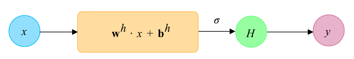
Figure 4.1. Schematic representation of the operations within a single MLP layer as presented in (4.1).

4.1. Residual network

The first variation in the network architecture we consider, originating from He et al. [26], is the residual network (ResNet), which is a slight modification of the classical MLP. This network architecture consists of layers with the following transformation

$$\mathbf{y}=H(\mathbf{x},W_{H})+\mathbf{x},$$ (4.2)

i.e. the input is added to the layer together with the non-linearity. A visual representation of this layer is provided in Figure 4.2.

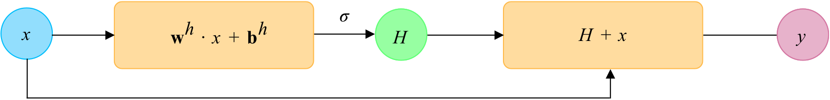
Figure 4.2. Schematic representation of the operations within a single residual layer as presented in (4.2).

This architecture provides an additional ‘channel’ which leaves the input vector $\mathbf{x}$ unaffected, allowing for the input vector $\mathbf{x}$ to flow through the layer, by adding it to the non-linear computation in the layer. The addition of this operation is minor, but can have large influence on the mean square error (MSE), as we will see in Section 5. He et al. [26] claim that this network has been particularly successful with complex images, when composed with convolutional neural networks.

4.2. Highway network

Highway networks are a generalization of the residual network architecture from the previous subsection, by introducing an additional non-linearity $T(\mathbf{x},W_{T})$, called the transform gate. This non-linearity will determine the amount of information flowing from the non-linearity $H$ inside the layer and the amount of information ‘carried’ over from the input vector $\mathbf{x}$. The outcome is thus the following transformation

$$\mathbf{y}=H(\mathbf{x},W_{H})\odot T(\mathbf{x},W_{T})+\mathbf{x}\odot\big{[}1-T(\mathbf{x},W_{T})\big{]},$$ (4.3)

where $\odot$ denotes the Hadamard product between vectors or matrices. Hence, $T$ creates a convex combination between the input $\mathbf{x}$ and the transformed input $H(\mathbf{x},W_{H})$ before the output. A visual representation of this layer is given in Figure 4.3.

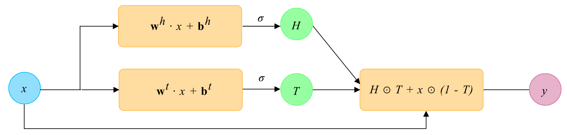
Figure 4.3. Schematic representation of the operations within a single highway layer as presented in (4.3).

In the approximation of complex functions using neural networks, the depth of the network is proven to be a significant factor in its success, see e.g. Telgarsky [40]. However, training deeper networks presents additional bottlenecks, such as the vanishing gradients problem. The intuition behind highway networks is to allow for unimpeded information flow across the layers; see Srivastava et al. [39]. Indeed, from equation (4.3) we can see that for the boundary values of $T$ we have

$$\mathbf{y}=\begin{cases}\mathbf{x},&T(\mathbf{x},W_{T})=\mathbf{0}\\ H(\mathbf{x},W_{H}),&T(\mathbf{x},W_{T})=\mathbf{1},\end{cases}$$ (4.4)

therefore

$$\frac{\mathrm{d}\mathbf{y}}{\mathrm{d}\mathbf{x}}=\begin{cases}I,&T(\mathbf{x},W_{T})=\mathbf{0}\\ H^{\prime}(\mathbf{x},W_{H}),&T(\mathbf{x},W_{T})=\mathbf{1},\end{cases}$$ (4.5)

where $I$ denotes the identity matrix. Thus, the transform gate $T$ allows the highway layer to vary its behavior between a standard MLP layer and an identity mapping, leaving $\mathbf{x}$ unaffected.

4.3. Generalized highway network

One can further generalize highway networks by removing the convexity requirement in the outcome. Let us define an additional non-linear transformation alongside $T(\mathbf{x},W_{T})$, which we call $C(\mathbf{x},W_{C})$, such that the outcome takes the form

$$\mathbf{y}=H(\mathbf{x},W_{H})\odot T(\mathbf{x},W_{T})+\mathbf{x}\odot C(\mathbf{x},W_{C}).$$ (4.6)

We call $T$ and $C$ the transform and carry gate, respectively, as they regulate the amount of information passed into the next layer from the transformed and original input. This gating mechanism allows for information to flow along the layers of the network without attenuation. Highway networks are obviously a special case of generalized highway networks, once we set $C=1-T$. A visual representation of this layer is given in Figure 4.4.

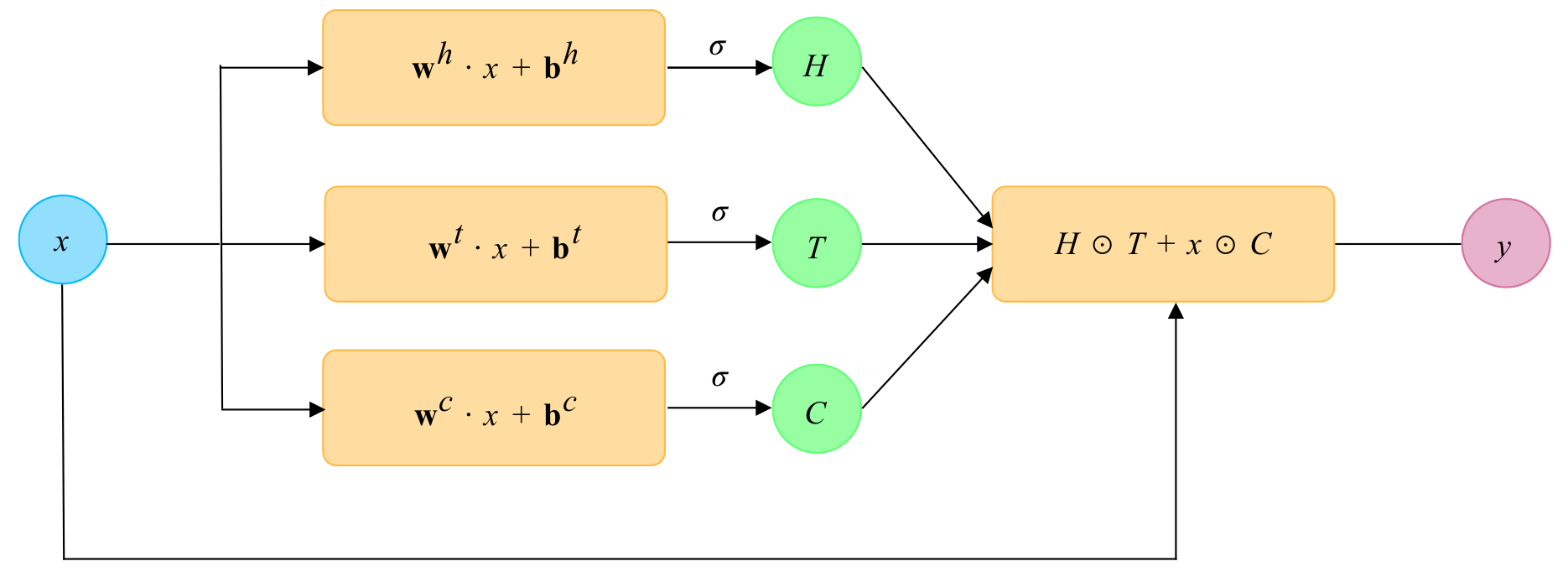
Figure 4.4. Schematic representation of the operations within a single generalized highway layer as presented in (4.6).

4.4. DGM network

The next network architecture we are interested in is the DGM network that was recently developed by Sirignano and Spiliopoulos [38] in the context of the Deep Galerkin Method for the solution of high-dimensional PDEs; see also Al-Aradi et al. [2]. The authors of [38] argue that this network architecture allows for ‘sharp turns’ in the target function, which can occur near the boundary and terminal condition of a PDE. In the following sections, we develop variations of this network architecture in order to understand the flexibility of this architecture, and attempt to find potential improvements.

The architecture of a DGM network is similar to that of highway networks, see Section 4.2, in that there exist transform and carry gates determining how much information from the previous layer should be carried over to the next layer. The DGM network consists of an arbitrary amount of layers, which we call DGM layers.

4.4.1. DGM layer

Let us start by describing a DGM layer, within which several operations are executed. A schematic view of this layer is provided in Figure 4.5.

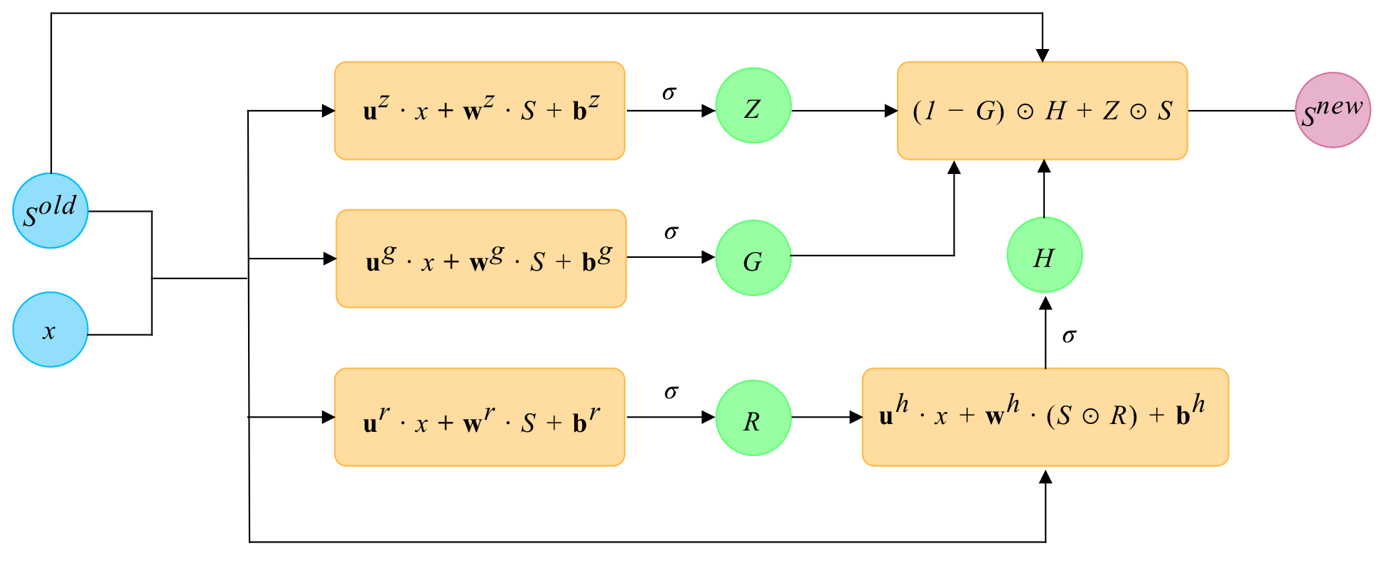
Figure 4.5. Schematic representation of the operations within a single DGM layer. Adopted from [2].

In contrast to a highway layer, the DGM layer has two inputs, $S^{old}$ and $\mathbf{x}$, denoted by blue in Figure 4.5. $S^{old}$ denotes the output from the previous layer. This can be either the first non-linear transformation $S^{1}$ or the output from another DGM layer; see Figure 4.6. Moreover, $\mathbf{x}$ denotes the original input vector, i.e. the ‘untouched’ feature data. We use both layer inputs to create $4$ vectors: $Z,G,R$ and $H$. Using these vectors, we compute $S^{new}$, the output of the DGM layer. The final operation in the layer equals

$$S^{new}=(1-G)\odot H+Z\odot S.$$ (4.7)

Let us set $T=1-G$, $C=Z$ and denote by $S$ the input to a highway layer, then we have a similar computation as in a generalized highway layer, i.e.

$$S^{new}=T\odot H+C\odot S,$$ (4.8)

where $H$ denotes the transformed input inside the layer and $S$ the output from the previous layer; compare with Section 4.2. A DGM layer features additional complexity compared to a highway layer in two ways:

• Instead of computing $H$ through one non-linear transformation as in a highway layer, we compute $H$ using two non-linear transformations, where the output of the first one is the input to the second one. This can be viewed as a ‘subnetwork’ inside the DGM layer. In Section 4.5 we exploit this property, by adding more non-linear transformations as a subnetwork to measure the relevance of this double transformation.

• In each non-linear transformation for the four vectors $Z,G,R,H$, the original feature vector $\mathbf{x}$ is incorporated. This leads to a recurrent architecture similar to recurrent neural networks; compare e.g. with Sherstinsky [36]. In Section 4.6, we create a DGM architecture without this feature, and train it alongside DGM to measure the impact of this recurrent architecture inside the layers.

Additionally, note the following about the DGM network architecture:

• As argued in [38], the incorporation of repeated element-wise multiplications of the nonlinear functions is useful in capturing sharp turns which can be present in complex functions. Because of the similarity of the DGM layer and the highway layer, we have that the input $\mathbf{x}$ enters into the calculations of each intermediate step, reducing the probability of vanishing gradients inside the back propagation phase of the training cycle.

• Due to the addition of more weight matrices and operations, a DGM layer contains roughly eight times as many parameters as an MLP layer. Additionally, four times as many activation functions are present in the network.

4.4.2. Overall DGM architecture

The DGM layer that we examined in Subsection 4.4.1 requires both $\mathbf{x}$ and some transformation $S$ as input, hence we must compute the transformation $S$ from the input before the layer. Additionally, we incorporate a final linear transformation to obtain the output $\mathbf{y}$. Therefore, the overall architecture of the DGM network is provided in Figure 4.6.

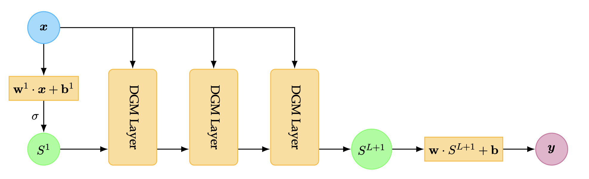
Figure 4.6. High level overview of the DGM network. Each DGM layer refers to the operations visualized in Figure 4.5. Adopted from [2].

This is again similar to a generalized highway network. Equation (4.6) requires the dimensionality of $\mathbf{x},\mathbf{y},H(\mathbf{x},W_{H})$ and $T(\mathbf{x},W_{T})$ to be equal. The result of this equality is that we cannot change the amount of nodes over chained highway layers. We must therefore use a dense layer to transform the input dimension to the dimension of the highway layers we want to use. A similar computation happens in the DGM architecture where we first compute

$$S^{1}=\textbf{w}^{1}\cdot\mathbf{x}+\textbf{b}^{1},$$ (4.9)

to regulate the dimension of $S^{1}$.

4.5. Deep DGM network

In this section, we consider a variant of the DGM network with multiple non-linear operations to compute $H$. A visualization of this network is presented in Figure 4.7.

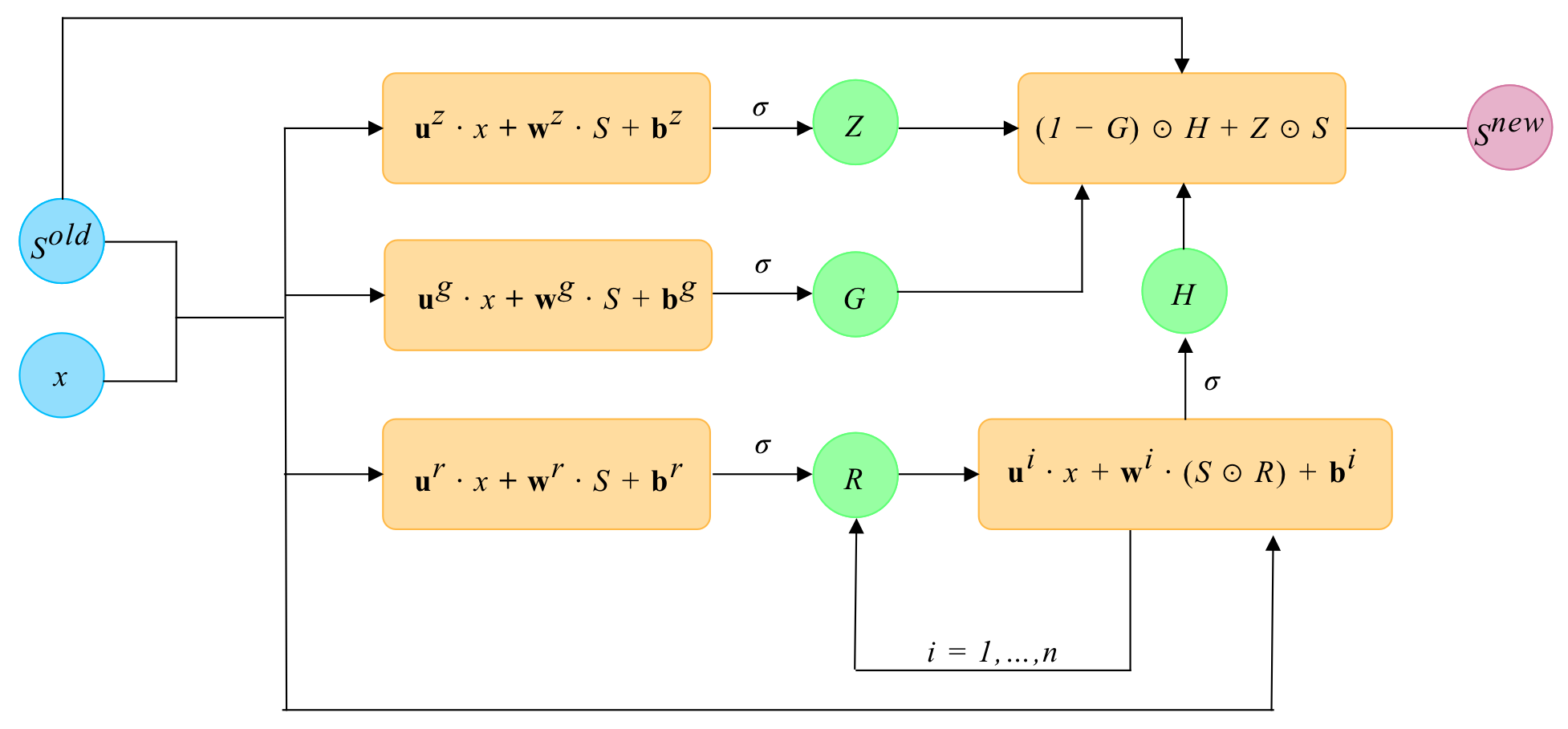
Figure 4.7. Schematic representation of the operations within a single deep DGM layer. In each layer, we have $n$ transformations.

In this network, we can vary the number of nonlinear operations performed on $R$ in order to obtain $H$ as a hyper-parameter. If we choose, for example, $n=5$, this means that $5$ additional weight matrices for both w, u and $\mathbf{b}$ are required, for a total of $10$ additional weight matrices and $5$ bias vectors and non-linear functions. A deep DGM layer is therefore considerably more complex than the ‘standard’ DGM layer. The goal of this network is to quantify the influence of deeper non-linearities within a DGM layer.

4.6. No-Recurrence DGM network

The network in which we omit the dependence on $\mathbf{x}$ in all the layers apart from the input layer is a simplified version of the DGM network. A visualization of this network architecture is available in Figure 4.8. Note that none of the operations depends on $\mathbf{x}$, greatly reducing the amount of parameters each layer contains as we do not require weight matrices w for all the layer dependencies on $\mathbf{x}$.

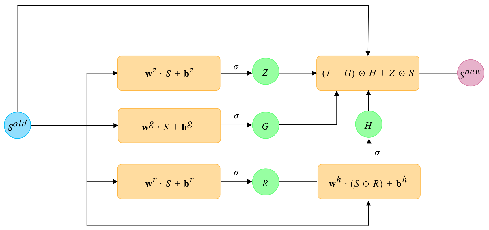
Figure 4.8. Schematic representation of the operations within a single no-recurrence DGM layer.

The structure of this layer closely resembles a highway layer; compare with Section 4.2. Indeed, the only notable difference is the way we compute $H$:

$$H=\sigma\Big{(}\textbf{w}^{h}\cdot\Big{[}S\cdot\sigma\left(\textbf{w}^{r}\cdot S+\textbf{b}^{r}\right)\Big{]}+\textbf{b}^{h}\Big{)},$$ (4.10)

whereas we have the following operation for $H$ in the highway layer

$$H=\sigma\left(\textbf{w}^{r}\cdot S+\textbf{b}^{r}\right).$$ (4.11)

5. Problems revisited and data sampling

In this section, we take another look at the problems considered in this work and present the form that will be used in the empirical analysis. We also discus the methods for generating data and the parameter sets used for the training of the neural networks.

5.1. Black–Scholes and Heston models

The first problem we consider is the pricing of European call options in the Black–Scholes model. Let us define the following variables, from which we will sample later:

• $m=\frac{S}{K}$: the moneyness value;

• $\sigma$: the volatility of the underlying asset;

• $r$: the risk-free rate;

• $\tau=T-t$: a time transformation to obtain the time to maturity, in years.

Using these variables, we can calculate the price of a European call option using a transformed version of (2.2):

$$\begin{split}\pi_{t}(C;m,\tau,\sigma)&=\frac{\pi_{t}(C;K,T,\sigma)}{K}=m\Phi(d_{1})-\mathrm{e}^{-r\tau}\Phi(d_{2}),\\ d_{1}&=\frac{\log(m)+(r+\frac{1}{2}\sigma^{2})\tau}{\sigma\sqrt{\tau}}=d_{2}+\sigma\tau.\end{split}$$ (5.1)

When we train neural networks to compute call option prices in the Black–Scholes model, we will use the solution presented in (5.1).

In addition to the Black–Scholes pricing problem, we also train neural networks to compute the price of European call options in the Heston stochastic volatility model (2.4). The prices of call options in the Heston model are computed using the COS method and utilizing the affine structure of the characteristic function. We use this problem in order to investigate whether the various networks show consistent performance across different option pricing problems or not.

5.2. Implied volatility

The next problem we consider is the training and evaluation of neural networks for the computation of the implied volatility, thus continuing the analysis of Liu et al. [30], in which only MLPs are trained and evaluated. In addition to the standard dataset for the computation of the implied volatility, in which we use the parameters directly from the inverted Black–Scholes pricing problem (Table 5.3), we also apply a transformation on the dataset from the scaled call price $(\pi/K)$ to the scaled time value of the option, already introduced in Liu et al. [30]. The reasoning behind this transformation is the following: We train the networks to find the solution to equation (2.3). However, we know that the option’s vega, i.e. its derivative with respect to the volatility, can become arbitrarily small for deep in-the-money (ITM) or deep out-of-the-money (OTM) options. In the context of neural networks, where we take the derivatives to compute the gradient of the network, the instability of vega may lead to large gradients, possibly causing significant estimation errors.

Let us briefly elaborate further on this issue. We denote $\pi=:f(\sigma)$ for convenience, where $f$ is the analytical function representing the price of European call option in the Black–Scholes model, depending on $\sigma$. The implied volatility problem concentrates on approximating the inverse of this problem, i.e. $\sigma=f^{-1}(\pi)$. During the back propagation phase, we must compute the gradient of $f^{-1}(\pi)$ with respect to $\pi$. That is, $\frac{d\sigma}{d\pi}=\frac{1}{d\pi/d\sigma}$, which is the reciprocal of the vega. Hence, for arbitrarily small values of vega, this gradient will explode, leading to convergence problems.

In order to address this issue, we will follow the gradient-squash approach of Liu et al. [30]. An option value can be divided into its intrinsic value (i.e. the no-arbitrage bound) and its time value. In order to obtain the time value, we subtract the intrinsic value from the option value, yielding

$$\hat{\pi}_{t}=\pi_{t}-(S_{t}-K\mathrm{e}^{-r\tau})^{+},$$ (5.2)

where $\hat{\pi}$ denotes the time value. Finally, we will also apply a $\log$-transform to further reduce the possible steepness of the gradient, resulting in the dataset shown in Table 5.4.

5.3. Data sampling

We treat each problem discussed above as a supervised learning problem. In other words, we require inputs and outputs which we can feed to the network and calculate the loss function. We will follow the configuration outlined in Liu et al. [30] for all three problems. We will generate a total of $1$ million samples for each problem, which we split into an $80/20$ training and validation set. We will generate an additional $100$ thousand samples used for evaluation. When sampling from the space of input parameters, we can either define a joint distribution over the entire domain, or sample each variable separately. Both Liu et al. [30] and Papazoglou-Hennig [33] opt for Latin hypercube sampling (LHS), in which values are sampled from a joint distribution, resulting in a better representation of the parameter space; cf. McKay et al. [31]. Thus, in order to remain consistent with previous research, we use LHS in this work to generate the data as well.

Starting from the Black–Scholes pricing problem, we sample points using the parameters shown in Table 5.1, and use the analytical solution in equation (5.1) to obtain the output labels. We use the same sampling parameters as in [30, 33], allowing us to compare the network performances to results in both works at a later stage.

	Parameters	Range
Input	Moneyness: $S_{0}/K$	$[0.4,1.6]$
	Time to Maturity ($\tau=T-t$)	$[0.2,1.1]$
	Risk-free rate ($r$)	$[0.02,0.1]$
	Volatility ($\sigma$)	$[0.01,1.0]$
Output	Scaled call price ($\pi/K$)	$(0.0,0.9)$

Table 5.1. Black–Scholes data generating parameters, adopted from [30].

The Heston pricing problem obviously requires additional parameters, whose range is listed in Table 5.2. The range for these parameters is selected again in accordance with Liu et al. [30].

	Parameters	Range
Input	Moneyness: $S_{0}/K$	$[0.4,1.6]$
	Time to Maturity ($\tau=T-t$)	$[0.2,1.1]$
	Risk-free rate ($r$)	$[0.02,0.1]$
	Correlation ($\rho$)	$[-0.95,0.0]$
	Reversion speed ($\kappa$)	$[0,2.0]$
	Long term variance ($\bar{v}$)	$[0,0.5]$
	Volatility of volatility ($\gamma$)	$[0,0.5]$
	Initial variance ($v_{0}$)	$[0.05,0.5]$
Output	Call price ($\pi$)	$(0.0,0.67)$

Table 5.2. Heston data generating parameters, adopted from [30].

In the ‘default’ implied volatility problem, we reuse the Black–Scholes pricing data and switch the role of the volatility $(\sigma)$ and the scaled call price $(\pi/K)$ as input and output, obtaining the parameters listed in Table 5.3.

	Parameters	Range
Input	Moneyness: $S_{0}/K$	$[0.4,1.6]$
	Time to Maturity ($\tau=T-t$)	$[0.2,1.1]$
	Risk-free rate ($r$)	$[0.02,0.1]$
	Scaled call price ($\pi/K$)	$[0,0.71]$
Output	Volatility ($\sigma$)	$(0.05,1.0)$

Table 5.3. Implied volatility data generating parameters, adopted from [30].

Finally, we transform the implied volatility dataset by applying the transformation described in equation (5.2), along with a $\log$-transform. The domain of the transformed implied volatility dataset, where we used the scaled time value, is provided in Table 5.4.

	Parameters	Range
Input	Moneyness: $S_{0}/K$	$[0.4,1.6]$
	Time to Maturity ($\tau=T-t$)	$[0.2,1.1]$
	Risk-free rate ($r$)	$[0.02,0.1]$
	Scaled time value ($\log(\hat{\pi}/K)$)	$[-18.42,-0.95]$
Output	Volatility ($\sigma$)	$(0.01,1.0)$

Table 5.4. Transformed implied volatility data generating parameters, adopted from [30].

6. Empirical results

In this section, we train neural networks using the architectures discussed in Sections 3 and 4, and apply them to the three different problems outlined in Sections 2 and 5. We then compare the empirical performance of these networks against each other, with the aim of identifying an optimal network architecture for the solution of these and related problems. The implementation for every network was done using Google’s TensorFlow library for Python [1] and the empirical analysis was carried out utilizing the Delft High Performance Computing Center [13] facilities.

6.1. Multilayer perceptrons

We start by training a set of MLPs ranging from a very small network to a large network, with similar configurations. The goal is to evaluate the performance of this network architecture, as well as to determine whether the size of the network influences the performance over a fixed range of epochs. To this end, we define a set of twelve networks with configurations listed in Table 6.1. We fix the learning rate according to the optimal value found from the study conducted in Liu et al. [30]. The batch size is chosen as large as possible while keeping calculations on a CPU fast. We found that a batch size of $64$ works well for the supervised learning problems discussed in this work. Furthermore, each network in this work is trained for $200$ epochs on the entire training dataset. We found out that, in most cases, increasing the amount of training epochs is beneficial. However, due to the large amount of network architectures that must be trained, we decided to terminate training after $200$ epochs.

	Multilayer Perceptron (MLP)
Layers	$2,3$
Nodes per layer	$50,100,150,200,250,500$
Activation function	ReLU
Loss function	MSE
Learning rate	$10^{-5}$
Batch size	64

Table 6.1. Overview of MLP configurations.

We allocate exactly one CPU core from the DHPC [13] (Intel Xeon 3.0GHz) cluster to each model. Doing so allows us to measure the training time for each model and to compare the performance trade-off to the off-line training time. Since we are training relatively small networks, GPU training does not speed up the process in most cases, as the overhead of distributing across the cores is too large. All networks are trained on the Black–Scholes and Heston pricing problems as well as on the two implied volatility problems. The empirical results for each problem are discussed below.

6.1.1. Black–Scholes model

Figure 6.1 visualizes the training time alongside the MSE for each network on the test set. We can see a clear relationship between the size of the network, which is increasing on the horizontal axis, the reduction in MSE and the increase in training time. Indeed, increasing the network size decreases the MSE (red) and hence improves the accuracy of the estimation, while the cost associated with this improvement is visible through the increase in training time (blue).

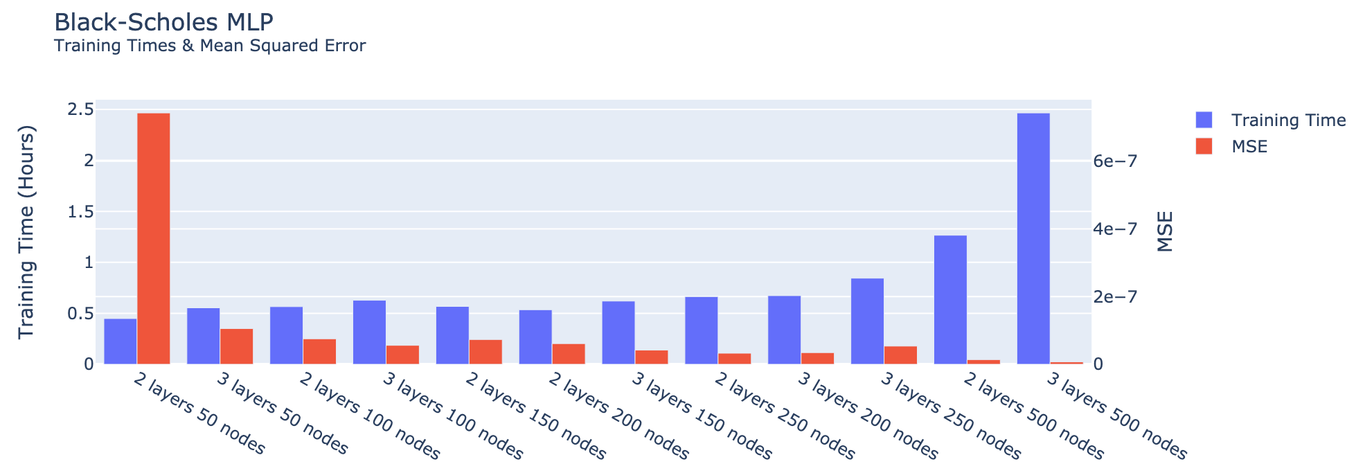
Figure 6.1. A comparison of the twelve networks from Table 6.1 including MSE on the test set (red) and training time (blue) for the Black–Scholes problem.

Interestingly, the performance increase of a larger network is not immediately visible during training. Figure 6.2 visualizes the training and validation losses over the $200$ training epochs for the $2$ layer networks with $50$ nodes (small), $250$ nodes (medium) and $500$ nodes (large). Notice that even though the largest network is almost $5$ times larger than the medium network and performs roughly $3.5$ times as well as the medium network, the training loss is almost identical for both networks. This is an indication that losses during training do not represent actual performance on unseen data. Additionally, the validation loss for the medium and large networks is lower than the training loss. This indicates a possible performance improvement for both networks if training time is extended for more epochs, which aligns with the results in Liu et al. [30]. Since the Black–Scholes problem has an analytical solution, we expect to be able to approximate the solution using neural networks to any degree of precision, when choosing an appropriately sized network along with many training cycles. The results from this section support this hypothesis. We select the $3$ layer $50$ node network to compare against the highway and DGM networks discussed later, as a good trade-off between accuracy and training time. Moreover, for the sake of completeness, we list the configuration of each network in Table 6.2, including training time and MSE; here, training time is measured in fractions of an hour.

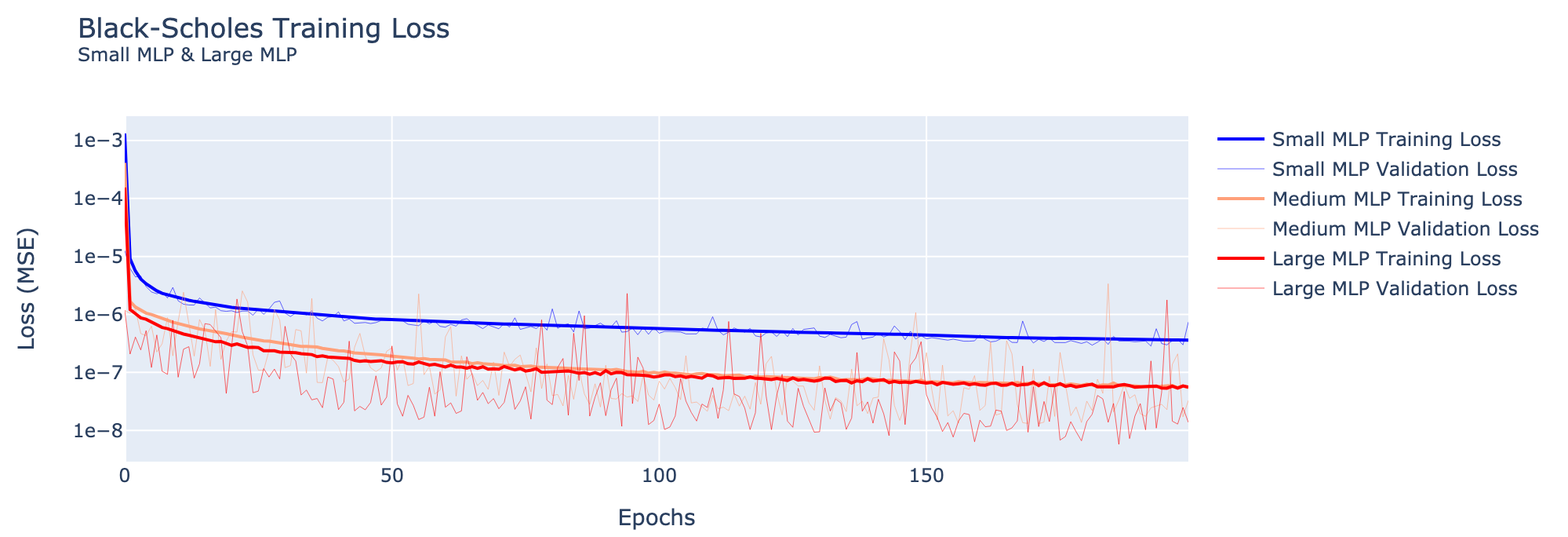
Figure 6.2. The training and validation losses for the three MLP networks. The small, medium and large networks contain $2,\!851$, $64,\!251$ and $504,\!001$ parameters respectively.

Model	Layers	Nodes	Parameters	Training Time (H)	MSE
1	$2$	$50$	$2,\!851$	$0.52$	$2.3\cdot 10^{-7}$
2	$2$	$100$	$10,\!701$	$0.57$	$7.5\cdot 10^{-8}$
3	$2$	$150$	$23,\!551$	$0.57$	$7.3\cdot 10^{-8}$
4	$2$	$200$	$41,\!401$	$0.54$	$6.1\cdot 10^{-8}$
5	$2$	$250$	$64,\!251$	$0.66$	$3.3\cdot 10^{-8}$
6	$2$	$500$	$253,\!501$	$1.27$	$1.4\cdot 10^{-8}$
7	$3$	$50$	$5,\!401$	$0.55$	$1.1\cdot 10^{-7}$
8	$3$	$100$	$20,\!801$	$0.63$	$5.6\cdot 10^{-8}$
9	$3$	$150$	$46,\!201$	$0.62$	$4.2\cdot 10^{-8}$
10	$3$	$200$	$81,\!601$	$0.67$	$3.4\cdot 10^{-8}$
11	$3$	$250$	$127,\!001$	$0.84$	$5.4\cdot 10^{-8}$
12	$3$	$500$	$504,\!001$	$2.47$	$7.0\cdot 10^{-9}$
MLP [33]	$6$	$200$	$202,\!201$	-	$1.3\cdot 10^{-7}$

Table 6.2. An overview of the MLP configurations alongside training time and MSE for the Black–Scholes problem. The best performing network (in MSE) is highlighted.

6.1.2. Heston model

The results of the various MLPs trained and evaluated on the Heston pricing problem are presented in Figure 6.3. Therein we observe that the results for the Heston pricing problem using the MLP network architectures align qualitatively with those for the Black–Scholes problem. Since both problems are very similar in nature and attempt to approximate the same quantity, the similarity in results is rather expected.

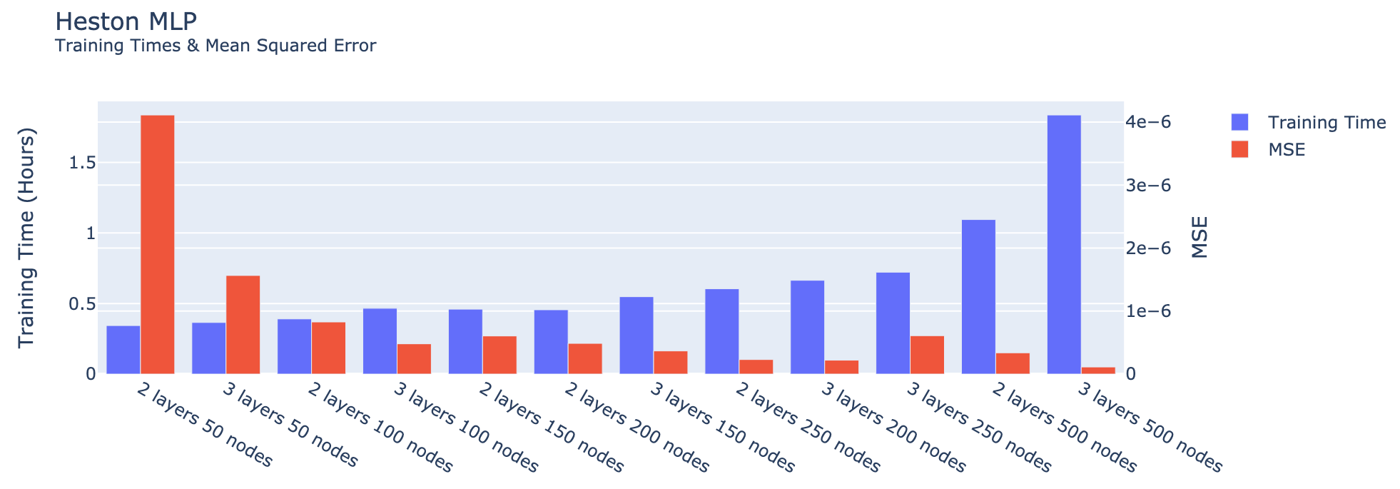
Figure 6.3. A comparison of the twelve networks from Table 6.1 including MSE on the test set (red) and training time (blue) for the Heston problem.

Indeed, the results from both the Black–Scholes as well as the Heston pricing problem exhibit, aside from the magnitude of the MSEs, many similarities; compare Figures 6.1 and 6.3. The MSEs and training times for the Heston model can be found in Table 6.3. The difference in MSEs is not surprising, as the Heston pricing problem has 8 parameters compared to the 4 parameters in the Black–Scholes problem.

Model	Layers	Nodes	Parameters	Training Time (H)	MSE
1	$2$	$50$	$3,\!051$	$0.34$	$4.1\cdot 10^{-6}$
2	$2$	$100$	$11,\!101$	$0.39$	$8.3\cdot 10^{-7}$
3	$2$	$150$	$24,\!151$	$0.46$	$6.0\cdot 10^{-7}$
4	$2$	$200$	$42,\!201$	$0.46$	$4.9\cdot 10^{-7}$
5	$2$	$250$	$65,\!251$	$0.60$	$2.3\cdot 10^{-7}$
6	$2$	$500$	$255,\!501$	$1.09$	$3.4\cdot 10^{-7}$
7	$3$	$50$	$5,\!601$	$0.37$	$1.6\cdot 10^{-6}$
8	$3$	$100$	$21,\!201$	$0.47$	$4.8\cdot 10^{-7}$
9	$3$	$150$	$46,\!801$	$0.55$	$3.7\cdot 10^{-7}$
10	$3$	$200$	$82,\!401$	$0.66$	$2.2\cdot 10^{-7}$
11	$3$	$250$	$128,\!001$	$0.72$	$6.1\cdot 10^{-7}$
12	$3$	$500$	$506,\!001$	$1.84$	$1.1\cdot 10^{-7}$
MLP [30]	$4$	$400$	$646,\!006$	-	$1.7\cdot 10^{-8}$

Table 6.3. An overview of the MLP configurations alongside training time and MSE for the Heston pricing problem. The best performing network (in MSE) is highlighted.

In Table 6.3, we observe that the MLP from [30] performs $10$ times better than the best performing MLP that we trained. We trained each network for $200$ epochs, whereas the authors of [30] train for $3000$ epochs. Since the architecture of the networks is identical, this indicates once again that longer training on this problem improves performance, similar to what we observed for the Black–Scholes pricing problem.

6.1.3. Implied volatility

The main observation for the implied volatility problem is that, contrary to the Black–Scholes and Heston problems, we cannot find evidence of larger networks performing better for this (inverse) problem. Indeed, the smallest network we train consists of $2$ layers and $50$ nodes per layer, containing a total of $2,\!851$ parameters, and performs just as well after $200$ epochs with identical configuration as the largest network with $3$ layers and $500$ nodes, containing $504,\!001$ parameters. Both networks have an MSE on the test set of $7.7\cdot 10^{-4}$, while the small network took only $0.4$ hours to train compared to the $2.17$ hours for the largest network. All networks show comparable performance, as can be seen in Figure 6.4.

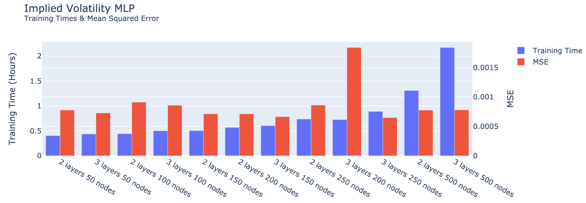
Figure 6.4. A comparison of the twelve networks from Table 6.1 including MSE on the test set (red) and training time (blue) for the implied volatility problem.

The identical performance of the networks during training is visualized in Figure 6.5. The results we find align with the errors found in [33], in which the best performing MLP network containing $202,\!201$ parameters performed worse on the test data than the considerably smaller networks from Figure 6.4. Table 6.4 lists all the networks along with the training times, amount of parameters and MSE for the implied volatility problem. The results indicate that the networks are dealing with convergence issues, preventing them to optimize further, regardless of their size and architecture.

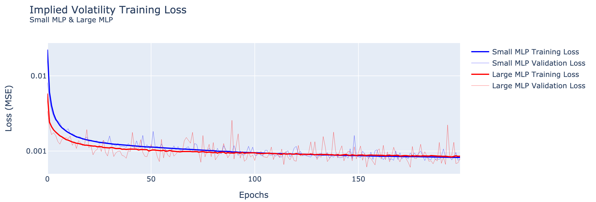
Figure 6.5. The training and validation loss of the smallest network compared to the largest network on the implied volatility data set.

Next, we consider the transformed implied volatility dataset, where we aim to solve the steep gradient problems possibly causing the convergence issues by introducing a transformation from the scaled call price to the scaled time value of the option, explained in Subsection 5.2.

Model	Layers	Nodes	Parameters	Training Time (H)	MSE
1	$2$	$50$	$2,\!851$	$0.40$	$7.7\cdot 10^{-4}$
2	$2$	$100$	$10,\!701$	$0.44$	$9.1\cdot 10^{-4}$
3	$2$	$150$	$23,\!551$	$0.50$	$7.1\cdot 10^{-4}$
4	$2$	$200$	$41,\!401$	$0.57$	$7.1\cdot 10^{-4}$
5	$2$	$250$	$64,\!251$	$0.74$	$8.6\cdot 10^{-4}$
6	$2$	$500$	$253,\!501$	$1.31$	$7.8\cdot 10^{-4}$
7	$3$	$50$	$5,\!401$	$0.44$	$7.3\cdot 10^{-4}$
8	$3$	$100$	$20,\!801$	$0.50$	$8.5\cdot 10^{-4}$
9	$3$	$150$	$46,\!201$	$0.60$	$6.6\cdot 10^{-4}$
10	$3$	$200$	$81,\!601$	$0.73$	$1.8\cdot 10^{-3}$
11	$3$	$250$	$127,\!001$	$0.94$	$7.6\cdot 10^{-4}$
12	$3$	$500$	$504,\!001$	$2.17$	$7.7\cdot 10^{-4}$

Table 6.4. An overview of the MLP configurations alongside training time and MSE for the implied volatility problem. The best performing network (in MSE) is highlighted.

Figure 6.6 visualizes the performances of the MLPs on the transformed implied volatility problem. We notice that on the transformed problem, the MSE is decreasing as a function of the network size, similarly to what we found for the option pricing problems before. The reduction in MSE is not as consistent as in the previous problems, indicating difficult convergence during training, possibly still due to a steep gradient not being entirely removed by the transformation. The results are considerably better than for the ‘default’ implied volatility problem, using only a simple transformation. Table 6.5 shows the results of all MLPs alongside their parameters and training times.

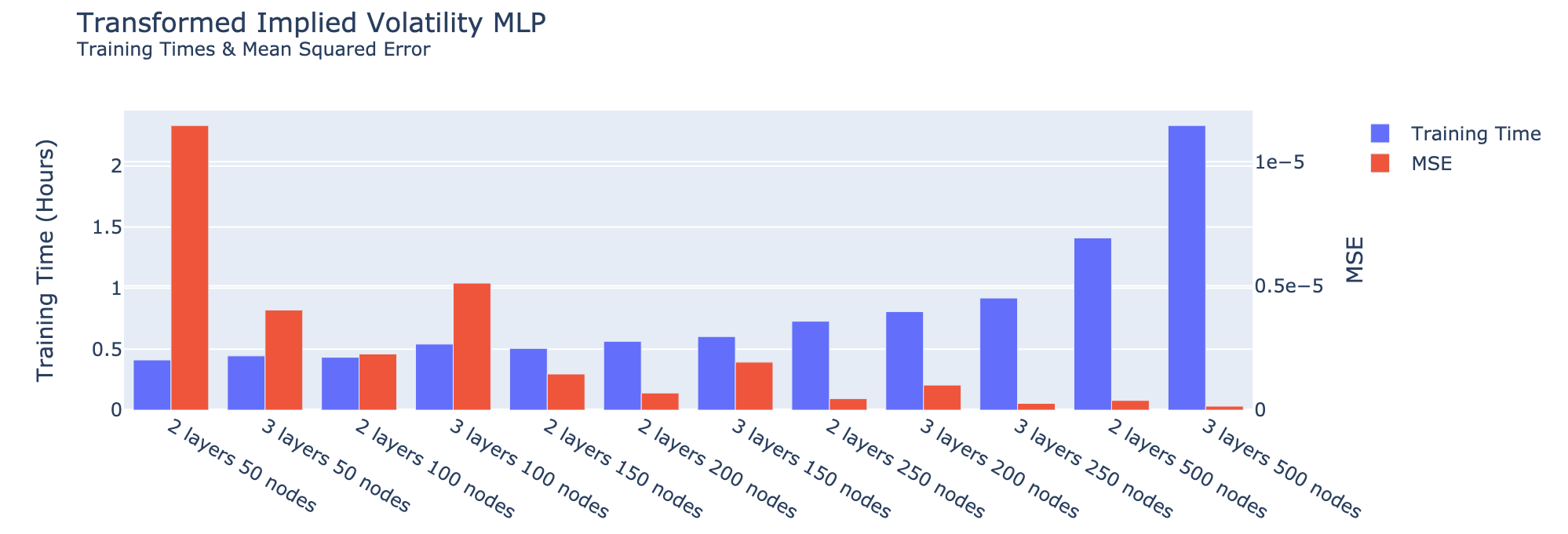
Figure 6.6. A comparison of the twelve networks from Table 6.1 including MSE on the test set (red) and training time (blue) for the transformed implied volatility problem.

Model	Layers	Nodes	Parameters	Training Time (H)	MSE
1	$2$	$50$	$2,\!851$	$0.41$	$1.1\cdot 10^{-5}$
2	$2$	$100$	$10,\!701$	$0.43$	$2.3\cdot 10^{-6}$
3	$2$	$150$	$23,\!551$	$0.51$	$1.5\cdot 10^{-6}$
4	$2$	$200$	$41,\!401$	$0.56$	$1.9\cdot 10^{-6}$
5	$2$	$250$	$64,\!251$	$0.73$	$6.9\cdot 10^{-6}$
6	$2$	$500$	$253,\!501$	$1.41$	$3.9\cdot 10^{-7}$
7	$3$	$50$	$5,\!401$	$0.44$	$4.0\cdot 10^{-6}$
8	$3$	$100$	$20,\!801$	$0.54$	$5.1\cdot 10^{-6}$
9	$3$	$150$	$46,\!201$	$0.60$	$1.9\cdot 10^{-6}$
10	$3$	$200$	$81,\!601$	$0.81$	$1.0\cdot 10^{-6}$
11	$3$	$250$	$127,\!001$	$0.92$	$2.7\cdot 10^{-7}$
12	$3$	$500$	$504,001$	$2.33$	$1.6\cdot 10^{-7}$

Table 6.5. An overview of the MLP configurations alongside training time and MSE for the transformed implied volatility problem. The best performing network (in MSE) is highlighted.

6.2. Highway networks

In this section, we train variants of the highway networks discussed in Section 4.2 with approximately equal configurations. More specifically, each network contains $3$ layers each with $50$ nodes. We train relatively small networks to compare across various architectures, in order to keep computational times feasible. Table 6.6 lists each highway network configuration.

	Generalized Highway	Highway	Residual
Layers	$3$	$3$	$3$
Nodes per layer	$50$	$50$	$50$
Total parameters	$23,\!251$	$15,\!601$	$7,\!951$
Initializer	Glorot Normal	Glorot Normal	Glorot Normal
Carry/Transform activation function	$\tanh$	$\tanh$	-
Activation function	$\tanh$	$\tanh$	$\tanh$
Loss function	MSE	MSE	MSE
Learning rate	$10^{-5}$	$10^{-5}$	$10^{-5}$
Batch size	$64$	$64$	$64$

Table 6.6. Overview of highway network configurations.

6.2.1. Black–Scholes model

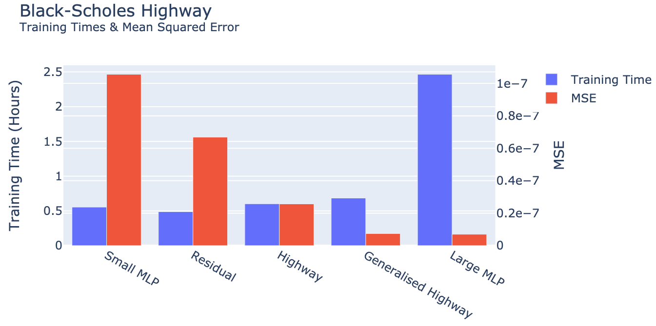
Figure 6.7. A comparison of highway networks from Table 6.6 including the smallest and largest MLP with the MSE on the test set (red) and training time (blue) for the Black–Scholes problem. The small MLP contains $3$ layers with $50$ nodes, and the large MLP $3$ layers with $500$ nodes. The results are ordered by the total number of parameters.

Figure 6.7 visualizes the training times (blue) and MSE on the test set (red) for each highway network. Both the highway and generalized highway networks perform better than their MLP counterpart with an equal amount of nodes. More impressive, however, is the fact that both networks required barely more training time than the small MLP, but scored comparably to the large MLP on the test set. This means that the highway architecture improves convergence on the Black–Scholes problem significantly. The difference in convergence speed can also be seen during training, as shown in Figure 6.8. In this case, training losses are a good indicator for performance on the test set, likely because the performance difference for both networks is so large. The loss during training is roughly one order of magnitude smaller for the generalized highway model compared to the MLP, whereas the training time is only $23\%$ longer; cf. Table 6.7.

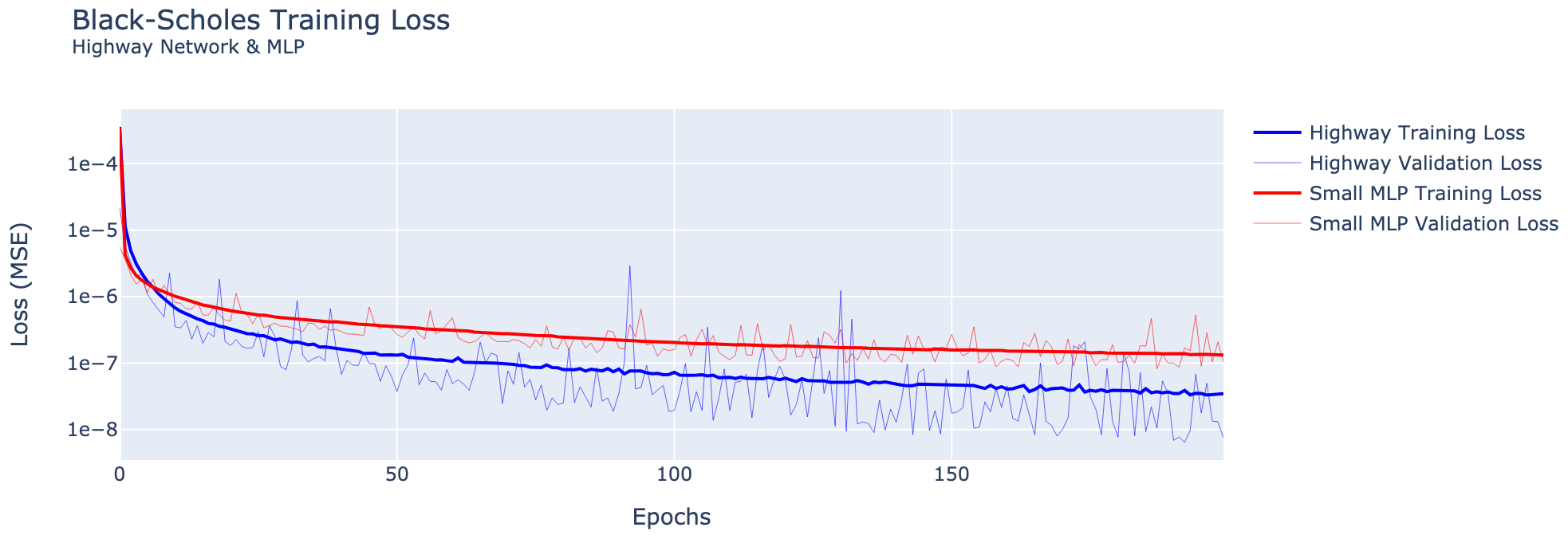
Figure 6.8. The training and validation loss over $200$ epochs. The small MLP consisting of $3$ layers and $50$ nodes ($2,851$ parameters) in red, compared to the $3$ layer $50$ node generalized highway network ($23,251$ parameters) in blue.

The residual layer is closest to the classical dense layer. The only difference is the carry of the input $\mathbf{x}$ to the next layer, cf. (4.2). Surprisingly, only carrying the input vector to the next layer decreases the MSE on the test set by $33\%$ from $1.1\cdot 10^{-7}$ to $6.7\cdot 10^{-8}$. Since only one additional operation is added in each layer, the training time is almost identical. Sirignano and Spiliopoulos [38], in the context of solutions for PDEs, argue that including the input vector in many operations allows the network to make ‘sharper turns’, resulting in a more flexible network. We see that this feature becomes particularly useful also when approximating the Black–Scholes price.

The difference in performance between the highway network and the residual network is also significant. The incorporation of one extra weight matrix and one additional non-linear function multiplied with the input vector $\mathbf{x}$ in each layer, cf. (4.3), results in an MSE reduction of $61\%$ from the residual network’s $6.7\cdot 10^{-8}$ to the highway network’s $2.6\cdot 10^{-8}$. Adding one additional weight matrix $W_{C}$ and non-linearity $C$, yielding the generalized highway layer, improves MSE performance by another $61\%$ compared to the highway layer. An overview of the error reductions, training times and operations in each layer are given in Table 6.7.

	Time (H)	MSE	Reduction ($\%$)	Layer operation
MLP	$0.55$	$1.1\cdot 10^{-7}$	-	$H$
Residual	$0.55$	$6.7\cdot 10^{-8}$	$33\%$	$H+\mathbf{x}$
Highway	$0.60$	$2.8\cdot 10^{-8}$	$61\%$	$H\cdot T+\mathbf{x}\cdot(1-T)$
Generalized Highway	$0.68$	$7.4\cdot 10^{-9}$	$73\%$	$H\cdot T+\mathbf{x}\cdot C$

Table 6.7. An overview of the highway network performance and error reductions for the MLP and highway network architectures on the Black–Scholes pricing problem. The reductions in the fourth column are relative to the previous row.

Finally, we notice that a $23\%$ increase in training time from the small MLP to the generalized highway network leads to a reduction of the MSE by $99\%$. When comparing the results obtained for the highway networks to the results in Liu et al. [30, Table 6], in which a large MLP is trained and evaluated on identical data, we see that our small generalized highway network already outperforms the MLP. In fact, as shown in Table 6.10, the generalized highway network improves the MSE by $9.8\%$ while reducing the amount of parameters by more than $96\%$ compared to the MLP from [30].

6.2.2. Heston model

Figure 6.9 visualizes the performance of the highway networks for the Heston pricing problem. We observe again a similar behavior as in the Black–Scholes pricing problem; compare with Figure 6.7. Indeed, the highway and generalized highway networks perform comparably to the large MLP in terms of MSE, while requiring the training time of the small MLP. A major difference is the performance of the residual network, which reduced the MSE by $33\%$ compared to the MLP on the Black–Scholes problem; cf. Table 6.7. On the Heston pricing problem, we see no increases in performance. A possible explanation for this could be that the Heston pricing problem might be too involved for the residual architecture to make an improvement.

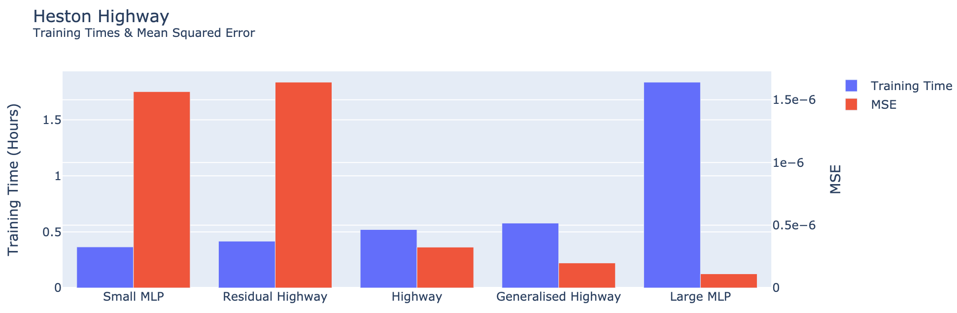
Figure 6.9. A comparison of highway networks from Table 6.6 including the smallest and largest MLP with the MSE on the test set (red) and training time (blue) on the Heston pricing problem. The small MLP contains $3$ layers with $50$ nodes, and the large MLP contains $3$ layers with $500$ nodes.

	Time (H)	MSE	Reduction ($\%$)	Layer Operation
MLP	$0.37$	$1.6\cdot 10^{-6}$	-	$H$
Residual	$0.42$	$1.7\cdot 10^{-6}$	$-5\%$	$H+\mathbf{x}$
Highway	$0.58$	$3.3\cdot 10^{-7}$	$80\%$	$H\cdot T+\mathbf{x}\cdot(1-T)$
Generalized Highway	$0.68$	$2.0\cdot 10^{-7}$	$39\%$	$H\cdot T+\mathbf{x}\cdot C$

Table 6.8. An overview of the highway network performance and error reductions for the MLP and highway network architectures on the Heston pricing problem. The reductions in the fourth column are relative to the previous row.

The highway and generalized highway networks do, in fact, improve the performance significantly compared to the MLP networks, with the generalized highway network performing almost as well as the largest MLP, while requiring only $31\%$ of the computational time. Table 6.8 lists the reductions that each highway variation contributes to the MSE. We notice that the improvement of the generalized highway network on the Heston problem is less significant than on the Black–Scholes problem, where the generalized highway network was the best performing network. In Section 6.3 we compare the highway networks to their DGM counterpart on the Heston pricing problem, and consider equally sized networks in terms of parameters.

6.2.3. Implied volatility

In the previous subsections, we found significant reductions in MSE on the test set when comparing the highway networks to the MLPs for the Black–Scholes and the Heston pricing problems. In this subsection, we perform the same comparison for the implied volatility problems. The results are visualized in Figure 6.10. In contrast to the Black–Scholes problem, in which the highway networks outperformed the MLPs, this is not the case for the implied volatility problem. None of the highway networks outperforms the MLPs on the test set. As in the MLP scenario, this indicates again that the steep gradient also poses a problem when optimizing the highway networks. In order to mitigate this issue, we consider the performance of the networks on the transformed implied volatility problem.

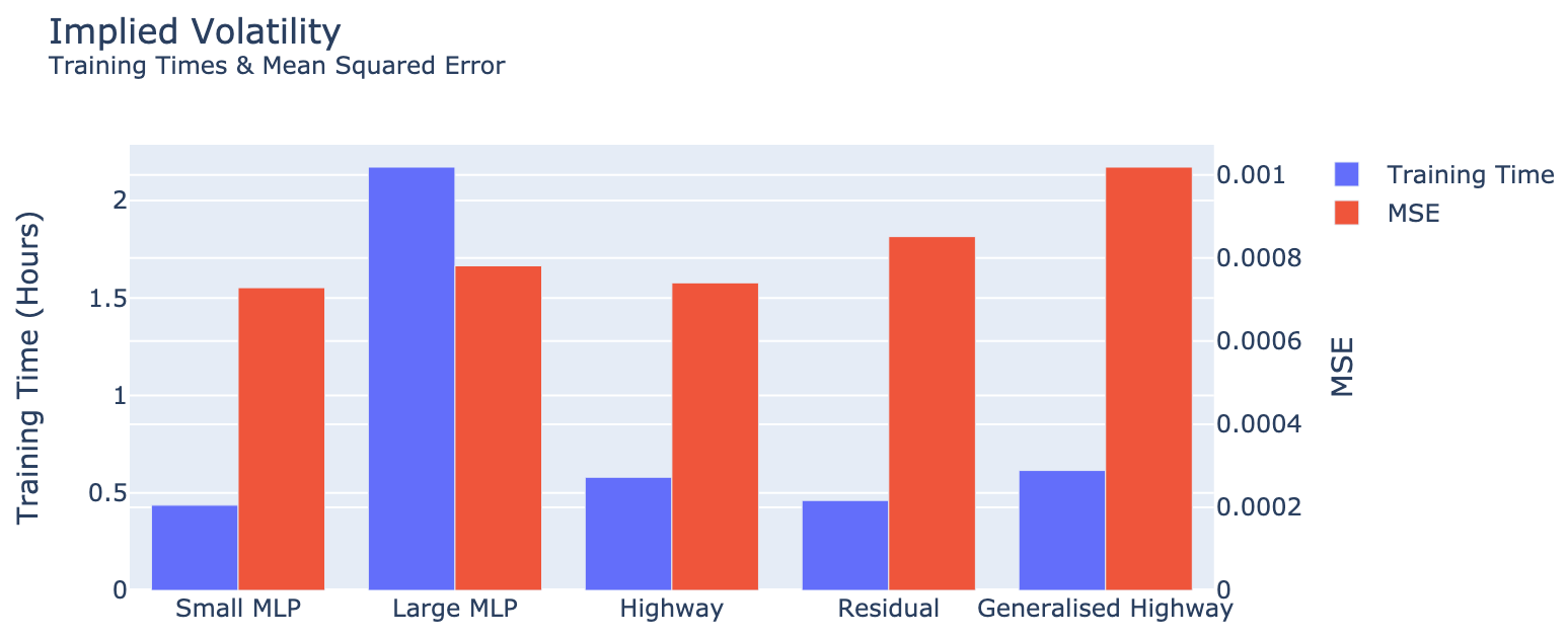
Figure 6.10. A comparison of the highway networks from Table 6.6 including the smallest and largest MLP with the MSE on the test set (red) and training time (blue) on the implied volatility problem. The small MLP contains $3$ layers with $50$ nodes and the large MLP contains $3$ layers with $500$ nodes.

In Figure 6.11 the performance of the highway networks on the transformed implied volatility dataset is shown. On this dataset, we find similar relative MSEs and computational times as for the Black–Scholes and Heston pricing problems. In fact, the generalized highway network is again the superior network relative to the training time. However, just like in the Heston pricing problem scenario, the large MLP scores lower in absolute MSE. This indicates that the network performance on the implied volatility problem is also prone to larger network sizes. We expect to see performance improvements when training highway networks with more nodes and layers.

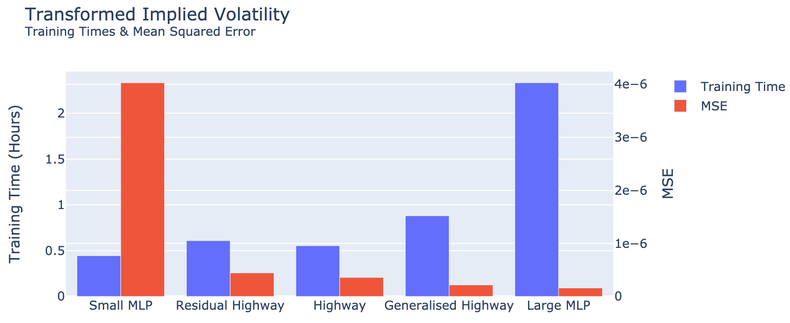
Figure 6.11. A comparison of the highway networks from Table 6.6 including the smallest and largest MLP with the MSE on the test set (red) and training time (blue) on the transformed implied volatility dataset. The small MLP contains $3$ layers with $50$ nodes and the large MLP contains $3$ layers with $500$ nodes.

These results clarify how much influence the network architecture has on the performance; consider, for example, the difference between the small MLP and the residual highway network. Recall that the operation of a residual network is simply the addition of the input vector to the layer; cf. (4.2). This operation reduces the MSE by roughly $89\%$, while adding only $38\%$ to the training time. We also notice that the training times for an identical network architecture can differ per dataset. In order to see this, consider the $14\%$ increase in training time from the small MLP to the residual network on the Heston problem (Table 6.8) and the $0\%$ increase on the Black–Scholes problem (Table 6.7).

6.3. DGM networks

In this section, we train the DGM network and its variations presented in subsections 4.4–4.6 and compare their performance to the highway and MLP networks. We train the DGM network with the configuration listed in Table 6.9.

	DGM Network
Layers	$3$
Nodes per layer	$50$
Total parameters	$33,\!459$
Activation function	$\tanh$
Initialiser	Glorot Normal
Loss function	MSE
Learning rate	$10^{-5}$
Batch size	64

Table 6.9. Overview of DGM network configurations.

6.3.1. Black–Scholes model

The results of the DGM network performance on the Black–Scholes problem are visualized in Figure 6.12. We note that more operations must be computed inside a DGM network than in a highway network, resulting in slightly more parameters and hence in longer training time. This aligns with the numerical results.

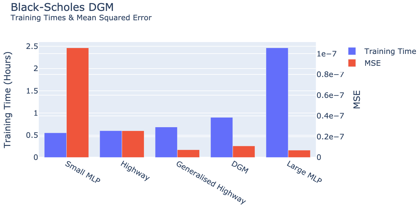
Figure 6.12. The MLP, highway and DGM networks compared in terms of MSE on the test set (red) and training time (blue) for the Black–Scholes pricing problem. The small MLP contains $3$ layers with $50$ nodes and the large MLP contains $3$ layers with $500$ nodes.

The main difference between the highway layer and the DGM layer is that the original input $\mathbf{x}$ is used in each DGM layer, whereas the highway layer only depends on the output of the previous layer. The dependence on $\mathbf{x}$ introduces $4$ additional weight matrices per layer; see Figure 4.5. In Figure 6.12 no significant improvements due to this dependence compared to the generalized highway network can be observed. Indeed, the generalized highway network has a smaller MSE and requires less computational time for training. Possibly, the Black–Scholes problem is not complex enough for the additional non-linearity and recurrence in the DGM layers to cause improvements. When comparing the DGM network to the MLP and highway network in the training phase, cf. Figure 6.13, we notice that the DGM network consistently outperforms the highway and MLP networks on the training and validation sets. This observation may suggest that the DGM network is more flexible and can fit the training data better, possibly leading to overfitting, resulting in underperformance on the test set compared to the generalized highway network.

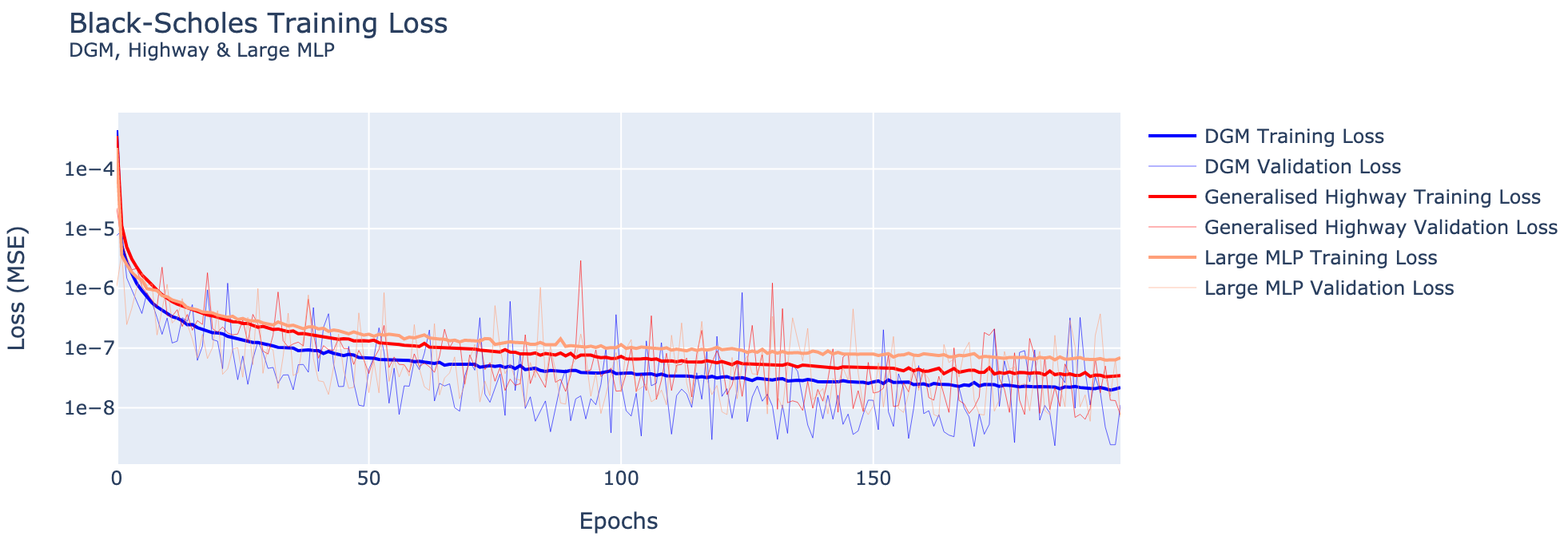
Figure 6.13. The MLP, highway and DGM networks compared during the training cycles.

In order to gain more insights into the impact of the operations inside the DGM network on the performance, we also train the deep DGM network and the no-recurrence DGM network with the same configuration as in Table 6.9, with the deep DGM layer containing $3$ sublayers. In Figure 6.14 the MSEs of the DGM variations are compared against the DGM and highway networks. As expected from the previous observations, the addition of sublayers inside the DGM layer, resulting in the deep DGM network (cf. subsection 4.5), does not bring significant performance improvements, while increasing training time by almost $50\%$ compared to the “plain” DGM network. Removing the dependence on the input vector $\mathbf{x}$ in all layers, resulting in the no-recurrence DGM network (cf. subsection 4.6), more than tripled the network error. This suggests that for the Black–Scholes pricing problem, the DGM network admits its performance benefits from the recurrence in the network.

The operations inside the no-recurrence network are very similar to those in a highway network. However, the MSEs on the test set are nowhere close. In order to verify that this was not a numerical issue, the no-recurrence network was trained multiple times, yielding similar results. The layer operations for the no-recurrence network and the generalized highway network after renaming weight matrices and activation functions are

$$\mathbf{y}=\Big{[}1-G(\mathbf{x},W_{G})\Big{]}\odot H\left(R(\mathbf{x},W_{R})\cdot\mathbf{x}\right)+Z(\mathbf{x},W_{Z})\odot\mathbf{x}$$ (6.1)

and

$$\mathbf{y}=\Big{[}1-Z(\mathbf{x},W_{Z})\Big{]}\odot H(\mathbf{x},W_{H})+Z(\mathbf{x},W_{Z})\odot\mathbf{x},$$ (6.2)

respectively. Hence, the difference in performance likely originates from the additional non-linearity $R$ or $G$. The fact that the introduction of two additional operations have such a negative influence in accuracy suggests that choosing an optimal network architecture can be a process subject to high sensitivity.

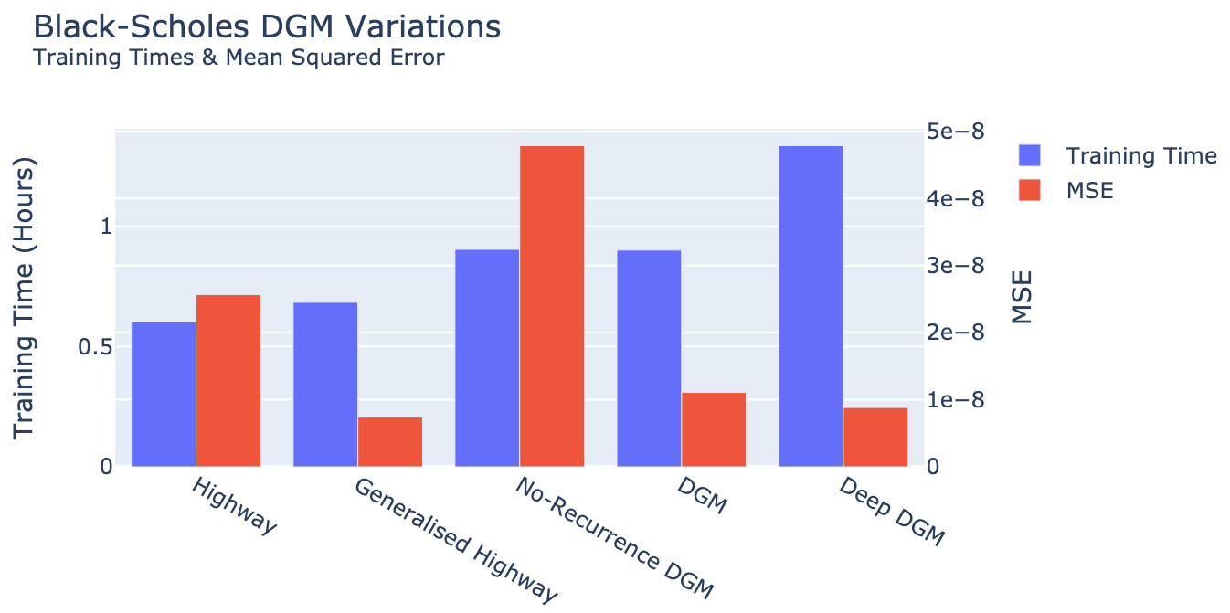
Figure 6.14. The highway and DGM networks, including DGM variations (deep DGM and no-recurrence DGM) compared in terms of MSE on the test set (red) and training time (blue) for the Black–Scholes pricing problem.

In addition, for the sake of completeness, Table 6.10 lists the Black–Scholes pricing MSE results for the most important networks, alongside the performance of the networks from [33, 30]. We notice that the generalized highway networks outperforms all other networks in terms of performance compared to total parameters and training time, and can be considered as the superior network.

Model	Layers	Nodes	Parameters	Training Time (H)	MSE
Small MLP	$3$	$50$	$5,401$	$0.55$	$1.1\cdot 10^{-7}$
Highway	$3$	$50$	$15,601$	$0.60$	$2.6\cdot 10^{-8}$
Generalized Highway	$3$	$50$	$23,251$	$0.68$	$7.4\cdot 10^{-9}$
No-Recurrence DGM	$3$	$50$	$31,059$	$0.90$	$4.8\cdot 10^{-8}$
DGM	$3$	$50$	$33,459$	$0.90$	$1.1\cdot 10^{-8}$
Deep DGM	$3$	$50$	$49,959$	$1.33$	$8.8\cdot 10^{-9}$
Large MLP	$3$	$500$	$504,001$	$2.47$	$7.0\cdot 10^{-9}$
MLP [33]	$6$	$200$	$202,201$	-	$1.3\cdot 10^{-7}$
DGM [33]	$5$	$100$	$210,601$	-	$1.6\cdot 10^{-7}$
MLP* [30]	$4$	$400$	$644,401$	-	$8.2\cdot 10^{-9}$
*Trained for $3000$ epochs, whereas the other networks are trained for $200$.

Table 6.10. An overview of MLP, highway and DGM network configurations alongside their training time and MSE for the Black–Scholes pricing problem. The best performing networks are highlighted. We also consider the networks from [33] and [30].

6.3.2. Heston model

In Figure 6.15 the performance of the DGM network alongside the smallest and largest $3$-layer MLPs and highway networks on the Heston pricing problem is shown. We notice that, unlike the Black–Scholes problem, the DGM network achieves a lower MSE than both the large MLP and the generalized highway network. The reason could be that the DGM has slightly more parameters which can lead to performance improvements.

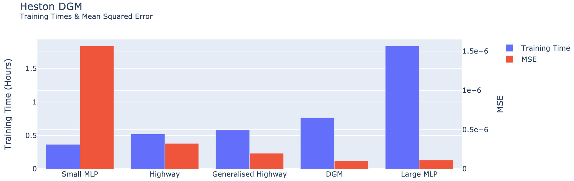
Figure 6.15. The highway and DGM networks compared in terms of MSE on the test set (red) and training time (blue) for the Heston pricing problem.

In order to validate this assumption, we train a highway network and a DGM network with approximately equal amount of parameters to the generalized highway network by varying the amount of layers. The configuration of these networks is shown in Table 6.11. The results are visualized in Figure 6.16. We can see that when the amount of parameters are comparable, the generalized highway network outperforms the highway and DGM network in both training time as well as in MSE. Hence, the reason the DGM network is performing better in Figure 6.15 is likely due to the increased number of parameters. We can conclude that the generalized highway network also performs well for the Heston price problem, when the amount of parameters is increased. The improvement in MSE with respect to the DGM network is marginal, but the computational time required for training a generalized highway network is considerably smaller.

	Highway	Generalized Highway	DGM
Layers	$4$	$3$	$2$
Nodes per layer	$50$	$50$	$50$
Total arameters	$20,901$	$23,451$	$24,467$

Table 6.11. Layer configurations for the highway and DGM network, in order to have comparable amount of parameters.

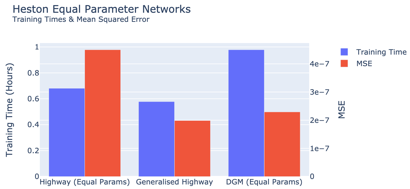
Figure 6.16. The highway, generalized highway and DGM networks where we compare the networks with comparable amounts of parameters on the Heston pricing problem. The generalized highway network performs best in both MSE and training time.

Finally, in Figure 6.17 the results of the deep DGM and the no-recurrence DGM networks are shown. We notice that neither the no-recurrence network nor the deep DGM network significantly improve performance or training time. Interestingly, the no-recurrence DGM also requires slightly longer training time, despite a fewer amount of parameters in the network, compared to the DGM network. We can conclude that the DGM network outperforms both variations. In addition, we find that while the recurrence in the DGM network has decreased the MSE, the additional complexity it brings along does not make it preferable for option pricing problems in the tested setup.

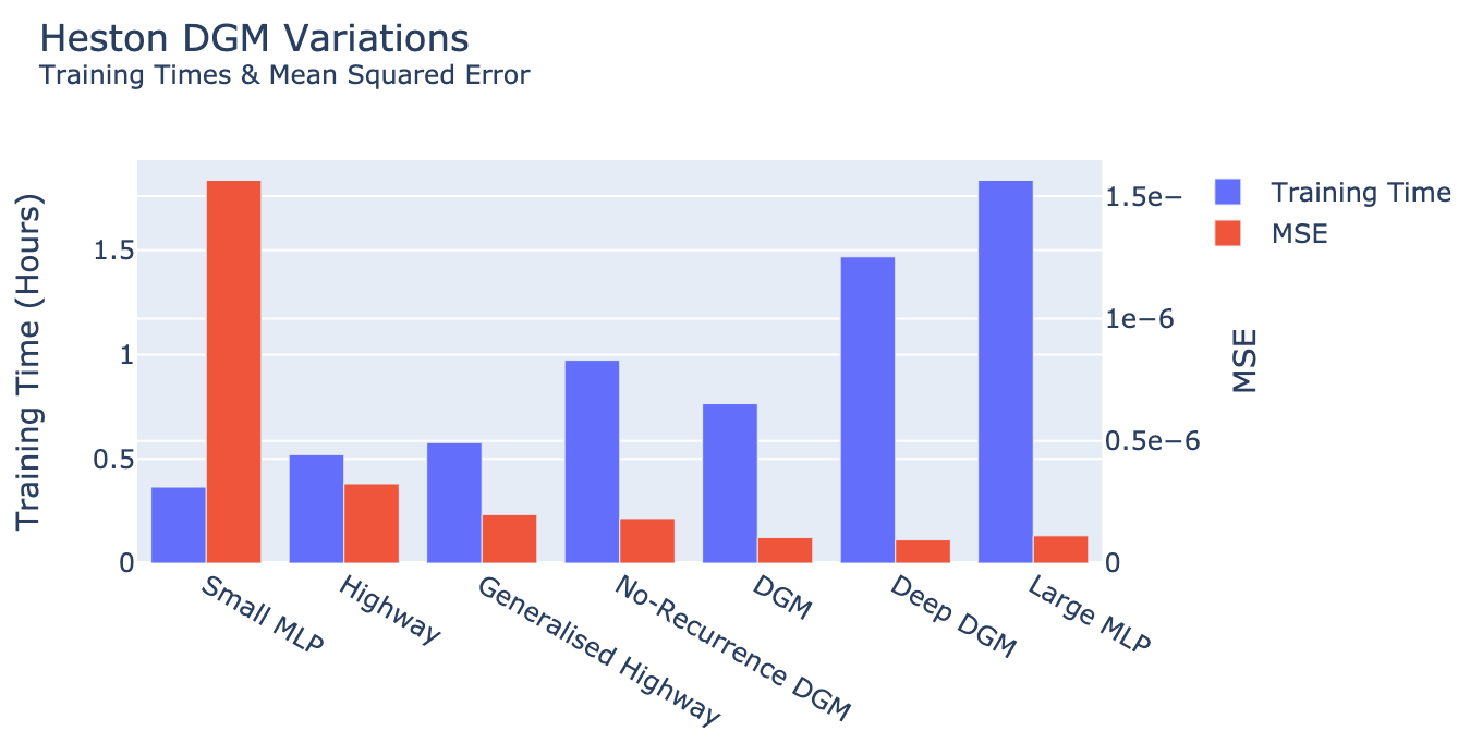
Figure 6.17. The highway and DGM networks, including DGM variations (deep DGM and no-recurrence DGM) compared in terms of MSE on the test set (red) and training time (blue) for the Heston pricing problem.

Concluding, we find that the generalized highway network outperforms all other networks in terms of performance compared to total parameters and training time, and can be considered as the superior network for the Heston pricing problem, similarly to the Black–Scholes problem.

6.3.3. Implied volatility

Finally, we examine the performance of the DGM networks on the implied volatility problem. We have seen in the previous subsections that the implied volatility problem has not been susceptible to performance increases with different architectures, which is likely due to the steep gradient problem present in the ‘default’ implied volatility formulation. We again find this result when considering the DGM networks. Table 6.12 lists the training times and MSE on the implied volatility problem for the networks considered in Figure 6.18. We notice that the $3$ layer $150$ node MLP performs best in terms of MSE and training time. We find comparable performance from the networks trained in [33, 30].

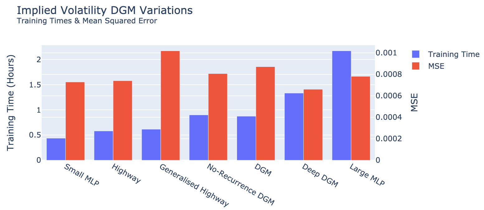
Figure 6.18. The highway, MLP and DGM network including DGM variations (deep DGM and no-recurrence DGM) compared in terms of MSE on the test set (red) and training time (blue) for the implied volatility problem.

Model	Layers	Nodes	Parameters	Training Time (H)	MSE
Small MLP	$3$	$50$	$5,401$	$0.44$	$7.3\cdot 10^{-4}$
Highway	$3$	$50$	$15,601$	$0.51$	$7.4\cdot 10^{-4}$
Generalized Highway	$3$	$50$	$23,251$	$0.62$	$1.0\cdot 10^{-3}$
No-Recurrence DGM	$3$	$50$	$31,059$	$0.90$	$8.1\cdot 10^{-4}$
DGM	$3$	$50$	$33,459$	$0.87$	$8.7\cdot 10^{-4}$
Best MLP	$3$	$150$	$46,201$	$0.60$	$6.6\cdot 10^{-4}$
Deep DGM	$3$	$50$	$49,959$	$1.33$	$6.6\cdot 10^{-4}$
Large MLP	$3$	$500$	$504,001$	$2.17$	$7.8\cdot 10^{-4}$
MLP [33]	$6$	$200$	$202,201$	-	$8.1\cdot 10^{-4}$
DGM [33]	$5$	$100$	$210,601$	-	$6.5\cdot 10^{-4}$
MLP* [30]	$4$	$400$	$644,401$	-	$6.4\cdot 10^{-4}$
*Trained for $3000$ epochs, whereas the other networks are trained for $200$.

Table 6.12. An overview of MLP, highway and DGM network configurations along with training time and MSE for the implied volatility problem. The best performing networks are highlighted. We also consider the networks from [33] and [30].

Since the results we find on the implied volatility dataset is probably a result of convergence problems originating from the formulation, we consider the DGM performance on the transformed implied volatility problem in the remainder of this section. We observed in subsection 6.2 that the highway architectures showed strong signs of decreased MSE with little increase in training time. Figure 6.19 shows the results of the DGM alongside the highway and MLP reference networks.

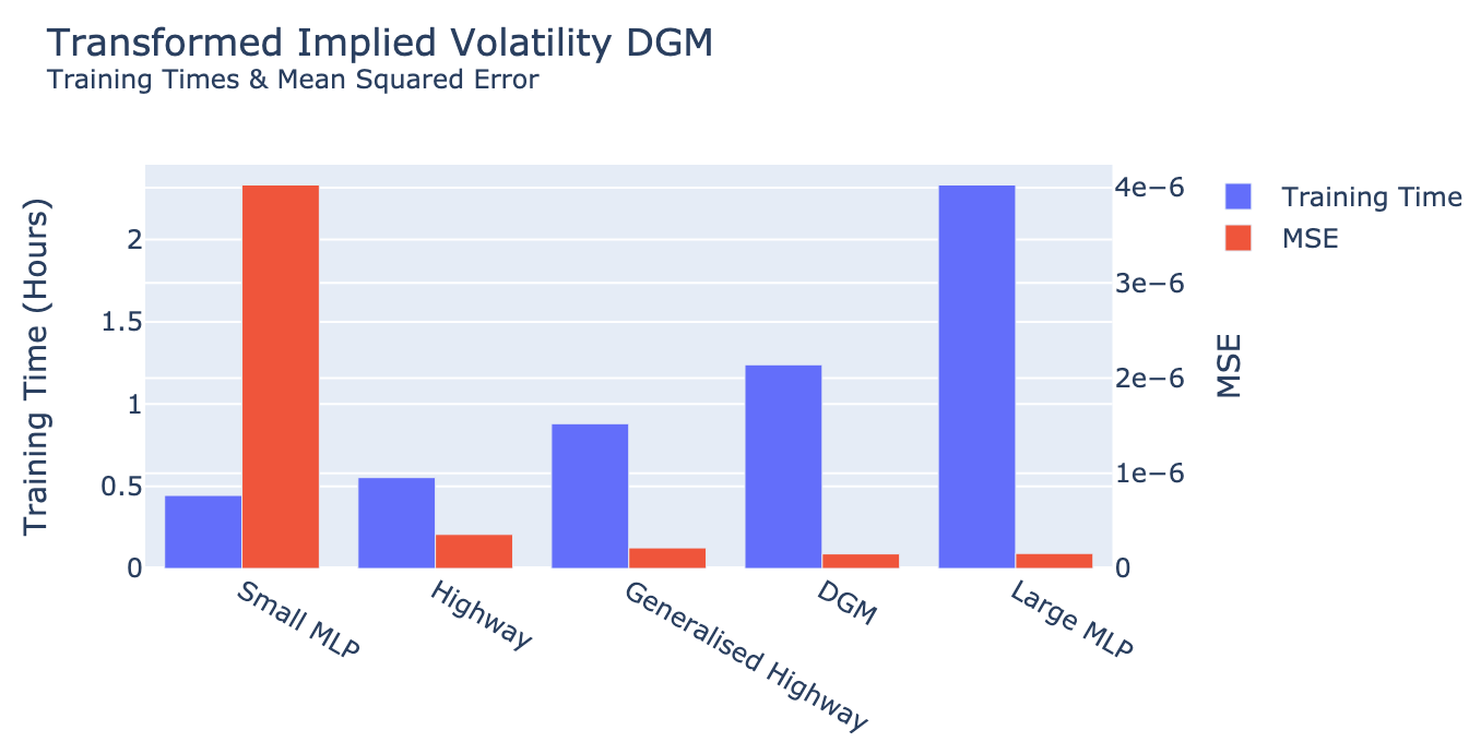
Figure 6.19. The highway, MLP and DGM networks compared in terms of MSE on the test set (red) and training time (blue) for the transformed implied volatility problem.

We notice that, similar to the Heston pricing problem, the DGM network outperforms the other networks in terms of absolute MSE. However, the generalized highway network performs better when the training time is taken into account. Contrary to the Heston pricing problem, where we observed that when equating the amount of parameters in each network the generalized highway network was the superior network, we find that the DGM remains the better network architecture for the transformed implied volatility problem. Indeed, Figure 6.20 visualizes the MSE reduction of $35\%$ from the generalized highway network to the DGM network, only requiring a $25\%$ increase of computational time.

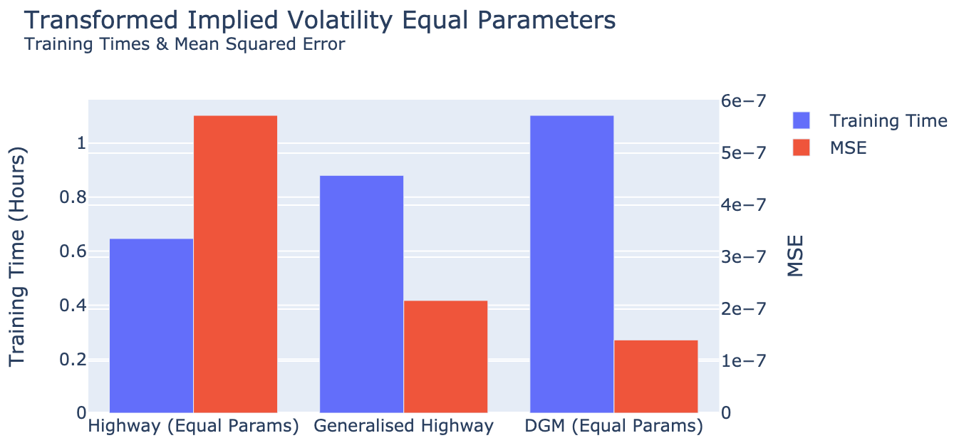
Figure 6.20. The highway, generalized highway and DGM networks where we compare the networks with comparable amounts of parameters on the transformed implied volatility problem.

When we also include the results of the DGM variations, see Figure 6.21, we find that the no-recurrence DGM shows even better performance than the DGM network. This network architecture is similar to the generalized highway architecture, but contains one additional non-linear operation. In all the previous problems, the additional non-linear operation caused reductions in performance compared to the simpler generalized highway architecture. However, for the transformed implied volatility problem, we observe that the no-recurrence architecture shows a $51\%$ reduction in MSE compared to the DGM network, and a $66\%$ reduction compared to the generalized highway. Table 6.13 shows the MSEs, training times and parameters for all the networks of interest. Taking the training times into account, we can concude that the no-recurrence DGM network is the superior network architecture for the implied volatility problem.

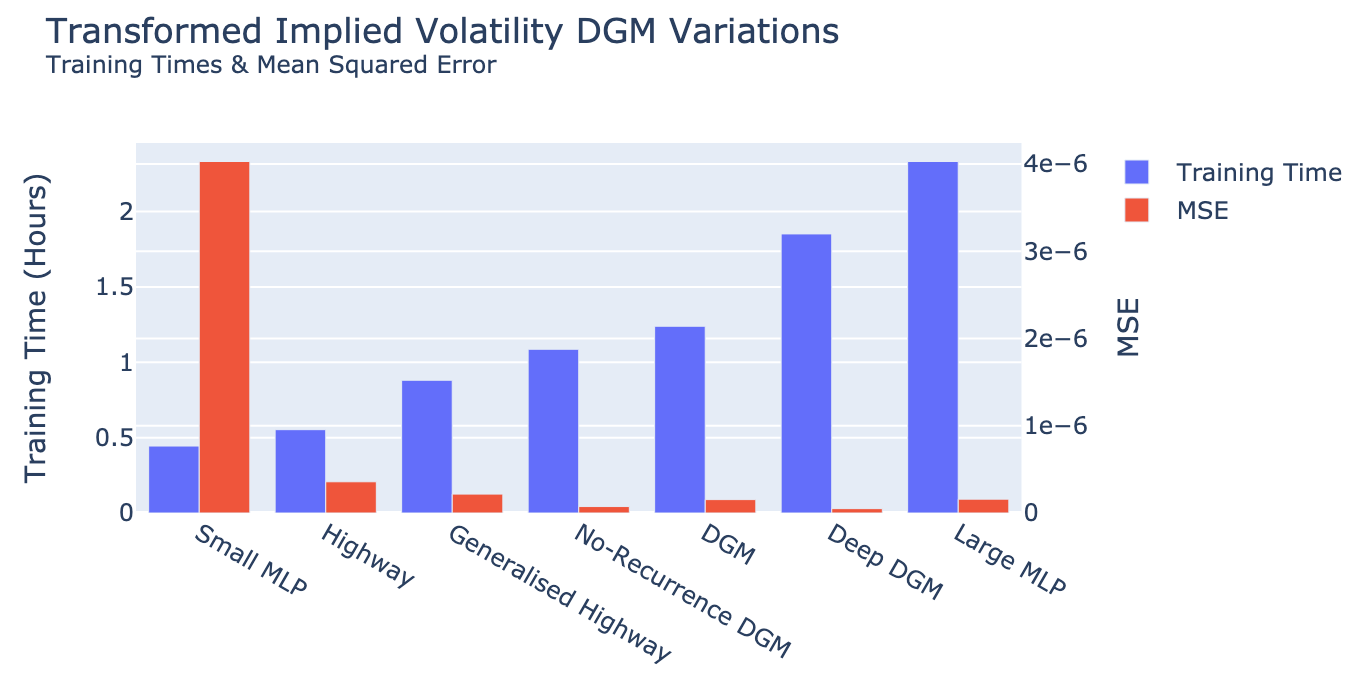
Figure 6.21. The highway, MLP and DGM networks including DGM variations (deep DGM and no-recurrence DGM) compared in terms of MSE on the test set (red) and training time (blue) for the transformed implied volatility problem.

Model	Layers	Nodes	Parameters	Training Time (H)	MSE
Small MLP	$3$	$50$	$5,401$	$0.44$	$4.0\cdot 10^{-6}$
Highway	$3$	$50$	$15,601$	$0.55$	$3.6\cdot 10^{-7}$
Generalized Highway	$3$	$50$	$23,251$	$0.88$	$2.2\cdot 10^{-7}$
No-Recurrence DGM	$3$	$50$	$31,059$	$1.09$	$7.4\cdot 10^{-8}$
DGM	$3$	$50$	$33,459$	$1.24$	$1.5\cdot 10^{-7}$
Deep DGM	$3$	$50$	$49,959$	$1.33$	$5.0\cdot 10^{-8}$
Large MLP	$3$	$500$	$504,001$	$2.33$	$1.6\cdot 10^{-7}$
MLP* [30]	$4$	$400$	$644,401$	-	$1.6\cdot 10^{-8}$
*Trained for $3000$ epochs, whereas the other networks are trained for $200$.

Table 6.13. An overview of MLP, highway and DGM network configurations along with training time and MSE for the implied volatility problem. The best performing networks are highlighted. We also consider the network from [30].

7. Conclusion

The empirical results from the numerical experiments conducted for this work, allow us to draw some practical conclusions that can assist us when choosing a neural network architecture for these and related problems in option pricing:

• The first observation is that increasing the number of parameters in the considered networks influenced the performance in the Black–Scholes, Heston and transformed implied volatility problems. We find that in many scenarios, increasing the amount of parameters in combination with a suitable architecture does in fact decrease the MSE and therefore increase the performance.

• We did not find evidence that losses during training were a good indicator for the performance of the network during evaluation. Instead, we found that networks performing well on the training data set did in no case outperform the other networks on the testing data (see e.g. the DGM network on the Black–Scholes pricing problem; Figures 6.12 and 6.13). We would have liked to see such a relationship, as it allows us to terminate the training cycle early when no improvement is made on the training set compared to other networks, saving valuable computational time.

• During training, the validation loss was often lower than the training loss. This indicates that we could possibly improve the accuracy of the networks by training them for more epochs. In Liu et al. [30], the results on the Heston pricing problem were more accurate, training for $3000$ cycles compared to $200$ in this work, while using an identical configuration for the MLPs.

• We observe that the generalized highway network architecture consistently outperformed the other networks for the Black–Scholes and Heston problems, when we compared the MSE relative to the computational time.

• In the case of the transformed implied volatility problem, we also found good performance results for the generalized highway network, which was however outperformed by the no-recurrence DGM architecture. This architecture is similar to the generalized highway network, but did not yield good results on the pricing problems.

• When training networks on the implied volatility dataset, we found poor performance for all networks, and no improvements when using more complex architectures. When transforming the dataset slightly, as explained in Section 5.2, the prediction accuracy increased significantly, and we found similar results in network architecture performance compared to the Black–Scholes and Heston pricing problems. This observation suggests that the training of networks is highly dependent on the formulation and the dataset. When training neural networks, we should try to ensure that gradients are bounded. A possible way to do this is to transform the input variables so that the gradient with respect to the input variables does not approach zero or infinity.

• Finally, we found that for the considered problems, the recurrent behavior of the DGM networks did not yield benefits when compared to the generalized highway networks. Instead, the computational complexity caused by the increase of operations inside the DGM layers made it less attractive in terms of relative performance to off-line required computational power than the generalized highway network.

References

- Abadi et al. [2015] M. Abadi, A. Agarwal, P. Barham, E. Brevdo, Z. Chen, C. Citro, G. S. Corrado, A. Davis, J. Dean, M. Devin, S. Ghemawat, I. Goodfellow, A. Harp, G. Irving, M. Isard, Y. Jia, R. Jozefowicz, L. Kaiser, M. Kudlur, J. Levenberg, D. Mané, R. Monga, S. Moore, D. Murray, C. Olah, M. Schuster, J. Shlens, B. Steiner, I. Sutskever, K. Talwar, P. Tucker, V. Vanhoucke, V. Vasudevan, F. Viégas, O. Vinyals, P. Warden, M. Wattenberg, M. Wicke, Y. Yu, and X. Zheng. TensorFlow: Large-scale machine learning on heterogeneous systems, 2015. URL https://www.tensorflow.org/.
- Al-Aradi et al. [2018] A. Al-Aradi, A. Correia, D. Naiff, G. Jardim, and Y. Saporito. Solving nonlinear and high-dimensional partial differential equations via deep learning. Preprint, arXiv:1811.08782, 2018.
- Bachouch et al. [2022] A. Bachouch, C. Huré, N. Langrené, and H. Pham. Deep neural networks algorithms for stochastic control problems on finite horizon: numerical applications. Methodol. Comput. Appl. Probab., 24(1):143–178, 2022.
- Bayer et al. [2021] C. Bayer, D. Belomestny, P. Hager, P. Pigato, and J. Schoenmakers. Randomized optimal stopping algorithms and their convergence analysis. SIAM J. Financial Math., 12(3):1201–1225, 2021.
- Bayer et al. [2023] C. Bayer, P. P. Hager, S. Riedel, and J. Schoenmakers. Optimal stopping with signatures. Ann. Appl. Probab., 33(1):238–273, 2023.
- Becker et al. [2019] S. Becker, P. Cheridito, and A. Jentzen. Deep optimal stopping. J. Mach. Learn. Res., 20:Paper No. 74, 25, 2019.
- Becker et al. [2021] S. Becker, P. Cheridito, A. Jentzen, and T. Welti. Solving high-dimensional optimal stopping problems using deep learning. European J. Appl. Math., 32(3):470–514, 2021.
- Black and Scholes [1973] F. Black and M. Scholes. The pricing of options and corporate liabilities. Journal of Political Economy, 81:637–654, 1973.
- Boudabsa and Filipović [2022] L. Boudabsa and D. Filipović. Machine learning with kernels for portfolio valuation and risk management. Finance Stoch., 26(2):131–172, 2022.
- Buehler et al. [2019] H. Buehler, L. Gonon, J. Teichmann, and B. Wood. Deep hedging. Quant. Finance, 19:1271–1291, 2019.
- Capponi and Lehalle [2023] A. Capponi and C. Lehalle, editors. Machine Learning and Data Sciences for Financial Markets: A Guide to Contemporary Practices. Cambridge University Press, 2023. doi: 10.1017/9781009028943.
- Cuchiero et al. [2020] C. Cuchiero, W. Khosrawi, and J. Teichmann. A generative adversarial network approach to calibration of local stochastic volatility models. Risks, 8(4), 2020.
- Delft High Performance Computing Centre [DHPC] Delft High Performance Computing Centre (DHPC). DelftBlue Supercomputer (Phase 1). https://www.tudelft.nl/dhpc/ark:/44463/DelftBluePhase1, 2022.
- Eberlein et al. [2010] E. Eberlein, K. Glau, and A. Papapantoleon. Analysis of fourier transform valuation formulas and applications. Applied Mathematical Finance, 17:211–240, 2010.
- Eckstein and Kupper [2021] S. Eckstein and M. Kupper. Computation of optimal transport and related hedging problems via penalization and neural networks. Appl. Math. Optim., 83(2):639–667, 2021.
- Eckstein et al. [2020] S. Eckstein, M. Kupper, and M. Pohl. Robust risk aggregation with neural networks. Math. Finance, 30(4):1229–1272, 2020.
- Eckstein et al. [2021] S. Eckstein, G. Guo, T. Lim, and J. Obłój. Robust pricing and hedging of options on multiple assets and its numerics. SIAM J. Financial Math., 12(1):158–188, 2021.
- Fang and Oosterlee [2008] F. Fang and C. W. Oosterlee. A novel pricing method for European options based on Fourier-cosine series expansions. SIAM Journal on Scientific Computing, 31:826–848, 2008.
- Fernandez-Arjona and Filipović [2022] L. Fernandez-Arjona and D. Filipović. A machine learning approach to portfolio pricing and risk management for high-dimensional problems. Math. Finance, 32(4):982–1019, 2022.
- Filipović [2009] D. Filipović. Term-Structure Models: A Graduate Course. Springer, 2009.
- Gatheral [2006] J. Gatheral. The Volatility Surface: A Practitioner’s Guide. Wiley, 2006.
- Georgoulis et al. [2023] E. H. Georgoulis, M. Loulakis, and A. Tsiourvas. Discrete gradient flow approximations of high dimensional evolution partial differential equations via deep neural networks. Commun. Nonlinear Sci. Numer. Simul., 117:Paper No. 106893, 11, 2023. ISSN 1007-5704. doi: 10.1016/j.cnsns.2022.106893. URL https://doi.org/10.1016/j.cnsns.2022.106893.
- Glorot and Bengio [2010] X. Glorot and Y. Bengio. Understanding the difficulty of training deep feedforward neural networks. In Y. W. Teh and M. Titterington, editors, Proceedings of the Thirteenth International Conference on Artificial Intelligence and Statistics, pages 249–256. PMLR, 2010.
- Han et al. [2018] J. Han, A. Jentzen, and W. E. Solving high-dimensional partial differential equations using deep learning. Proc. Natl. Acad. Sci. USA, 115(34):8505–8510, 2018.
- He et al. [2015] K. He, X. Zhang, S. Ren, and J. Sun. Delving deep into rectifiers: Surpassing human-level performance on imagenet classification. In 2015 IEEE International Conference on Computer Vision (ICCV), pages 1026–1034. IEEE Computer Society, 2015.
- He et al. [2016] K. He, X. Zhang, S. Ren, and J. Sun. Deep residual learning for image recognition. In 2016 IEEE Conference on Computer Vision and Pattern Recognition (CVPR), pages 770–778. IEEE Computer Society, 2016.
- Heston [1993] S. L. Heston. A closed-form solution for options with stochastic volatility with applications to bond and currency options. Review of Financial Studies, 6:327–343, 1993.
- Horvath et al. [2021] B. Horvath, A. Muguruza, and M. Tomas. Deep learning volatility: a deep neural network perspective on pricing and calibration in (rough) volatility models. Quant. Finance, 21:11–27, 2021.
- Huré et al. [2021] C. Huré, H. Pham, A. Bachouch, and N. Langrené. Deep neural networks algorithms for stochastic control problems on finite horizon: convergence analysis. SIAM J. Numer. Anal., 59(1):525–557, 2021.
- Liu et al. [2019] S. Liu, C. Oosterlee, and S. Bohte. Pricing options and computing implied volatilities using neural networks. Risks, 7:16, 1–22, 2019.
- McKay et al. [1979] M. D. McKay, R. J. Beckman, and W. J. Conover. A comparison of three methods for selecting values of input variables in the analysis of output from a computer code. Technometrics, 21:239–245, 1979.
- Neufeld and Sester [2023] A. Neufeld and J. Sester. A deep learning approach to data-driven model-free pricing and to martingale optimal transport. IEEE Trans. Inform. Theory, 69(5):3172–3189, 2023. ISSN 0018-9448.
- Papazoglou-Hennig [2020] J. Papazoglou-Hennig. Elementary stochastic calculus, application to financial mathematics, and neural network methods for financial models, 2020. Internship notes, NTUA-TUM.
- Pinelis and Ruppert [2022] M. Pinelis and D. Ruppert. Machine learning portfolio allocation. The Journal of Finance and Data Science, 8:35–54, 2022.
- Ruf and Wang [2020] J. Ruf and W. Wang. Neural networks for option pricing and hedging: a literature review. Journal of Computational Finance, 24(1):1–46, 2020.
- Sherstinsky [2020] A. Sherstinsky. Fundamentals of recurrent neural network (RNN) and long short-term memory (LSTM) network. Physica D: Nonlinear Phenomena, 404:132306, 28, 2020.
- Sirignano and Spiliopoulos [2018a] J. Sirignano and K. Spiliopoulos. DGM: a deep learning algorithm for solving partial differential equations. J. Comput. Phys., 375:1339–1364, 2018a. ISSN 0021-9991. doi: 10.1016/j.jcp.2018.08.029. URL https://doi.org/10.1016/j.jcp.2018.08.029.
- Sirignano and Spiliopoulos [2018b] J. Sirignano and K. Spiliopoulos. DGM: A deep learning algorithm for solving partial differential equations. Journal of Computational Physics, 375:1339–1364, 2018b.
- Srivastava et al. [2015] R. K. Srivastava, K. Greff, and J. Schmidhuber. Highway Networks. Preprint, arXiv:1505.00387, 2015.
- Telgarsky [2016] M. Telgarsky. Benefits of depth in neural networks. In V. Feldman, A. Rakhlin, and O. Shamir, editors, 29th Annual Conference on Learning Theory, pages 1517–1539. PMLR, 2016.
- Zhang et al. [2022] Z. Zhang, S. Zohren, and S. Roberts. Deep learning for portfolio optimization. The Journal of Financial Data Science, 2:8–20, 2022.