Toy model illustrating the effect of measurement dependence on a Bell inequality

Abstract

Bell’s inequalities rely on the assumption of measurement independence, namely that the probabilities of adopting configurations of hidden variables describing a system prior to measurement are independent of the choice of physical property that will be measured. Weakening this assumption can change the inequalities to accommodate experimental data. We illustrate this by considering quantum measurement to be the dynamical evolution of hidden variables to attractors in their phase space that correspond to eigenstates of system observables. The probabilities of adopting configurations of these variables prior to measurement then depend on the choice of physical property measured by virtue of the boundary conditions acting on the dynamics. Allowing for such measurement dependence raises the upper limit of the CHSH parameter in Bell’s analysis of an entangled pair of spin half particles subjected to measurement of spin components along various axes, whilst maintaining local interactions. We demonstrate how this can emerge and illustrate the relaxed upper limit using a simple toy model of dynamical quantum measurement. The conditioning of the hidden variable probability distribution on the chosen measurement settings can persist far back in time in certain situations, a memory that could explain the correlations exhibited in an entangled quantum system.

Bell inequalities arise from analysis of the statistics of purported ‘hidden variables’ that evolve according to local interactions and represent ‘elements of reality’ with definite values prior to measurement. It has been demonstrated that the inequalities can be violated, with recent experiments removing areas of uncertainty in the analysis such as the fair-sampling and locality loopholes [1, 2, 3, 4, 5, 6, 7]. Perhaps the most striking aspect of quantum mechanics is that its predictions are consistent with these violations. The implication is either that physical effects operate non-locally between space-like separated points, or that we have to abandon the concept of a reality independent of observation at microscopic scales [8, 9].

Should we wish to avoid these (arguably) unpalatable conclusions it is necessary to examine the assumptions made in Bell’s analysis, one of which is ‘measurement independence’, or ‘statistical independence’ [10], according to which the system prior to measurement is assumed to adopt states with probabilities that are independent of the measurement settings. A stronger version is that the prior state of a system should be capable of providing a measurement outcome for any system property.

We examine the effect of relaxing this assumption in the standard situation where two spin half particles in an entangled state have spin components separately measured along arbitrarily chosen axes. We demonstrate, by introducing measurement dependence, that the upper bound of the Clauser-Horne-Shimony-Holt (CHSH) parameter, $S(\hat{a},\hat{b},\hat{a}^{\prime},\hat{b}^{\prime})$, defined as [11]

$$S=|C(\hat{a},\hat{b})-C(\hat{a},\hat{b}^{\prime})|+|C(\hat{a}^{\prime},\hat{b})+C(\hat{a}^{\prime},\hat{b}^{\prime})|,$$ (1)

can be increased. $C(\hat{a},\hat{b})$ is the correlation function of spin component measurement outcomes $A$ and $B$ (each taking values $\pm$1) for particle 1 undergoing a spin measurement along axis $\hat{a}$ and particle 2 along axis $\hat{b}$, respectively, namely $C(\hat{a},\hat{b})=\overline{AB}=P_{++}^{\hat{a},\hat{b}}-P_{+-}^{\hat{a},\hat{b}}-P_{-+}^{\hat{a},\hat{b}}+P_{--}^{\hat{a},\hat{b}}$ where $P_{\pm\pm}^{\hat{a},\hat{b}}$ are the probabilities of measurement outcomes $A=\pm 1,B=\pm 1$ along the respective axes. Each correlation function takes a value between $\pm 1$ and $S$ could therefore lie between 0 and 4. However, assuming that the outcome of measurement of particle 2 is influenced neither by the choice of axis setting nor the outcome of measurement of particle 1, and vice versa, and also assuming that the system prior to measurement is specified by a set of hidden variables $\lambda$ adopted according to a probability density function (pdf) $\rho(\lambda)$, then $P_{\pm\pm}^{\hat{a},\hat{b}}=\int p_{1\pm}^{\hat{a}}(\lambda)p_{2\pm}^{\hat{b}}(\lambda)\rho(\lambda)d\lambda$ where $p_{1\pm}^{\hat{a}}(\lambda)$ are the probabilities of outcomes $\pm 1$ for the spin component of particle 1 along axis $\hat{a}$, for a given specification of hidden variables, with a similar meaning for $p_{2\pm}^{\hat{b}}(\lambda)$. Bell’s analysis requires $S$ to have an upper bound of 2. The crucial observation is that

$$|\bar{B}(\hat{b},\lambda)\!-\!\bar{B}(\hat{b}^{\prime},\lambda)|+|\bar{B}(\hat{b},\lambda)\!+\!\bar{B}(\hat{b}^{\prime},\lambda)|\leq 2,$$ (2)

where $\bar{B}(\hat{b},\lambda)=p_{2+}^{\hat{b}}(\lambda)-p_{2-}^{\hat{b}}(\lambda)$ is the mean outcome of measurement of the spin component of particle 2 along axis $\hat{b}$ for a given set of hidden variables $\lambda$. Note also that $|\bar{B}(\hat{b},\lambda)|\leq 1$. It has been shown that this upper bound can be violated experimentally.

Measurement independence is the use in the analysis of a pdf $\rho(\lambda)$ that depends neither on the measurement axes nor the outcome of the measurement. This can seem reasonable unless we entertain the view that measurement is a dynamical process. The usual alternatives to this are the classical acquisition of information without changing the system state, or the quantum mechanical instantaneous projection of the system to one of the eigenstates of the measured property. Instead, it could conceivably involve the evolution of hidden variables, that specify the states of the system and a coupled measuring device, towards attractors in their phase space that correspond to system eigenstates and device readings correlated with those eigenstates. This would create a relationship between initial state probabilities and the final measurement outcomes that act as boundary conditions. We could also imagine that deterministic rules could govern the evolution of the complete set of hidden variables while those describing the system alone could evolve stochastically, reflecting uncertainty in the initial state of the measuring device.

This point of view suggests that probabilities of hidden variable configurations might reasonably be conditioned on events taking place in the future, also known as ‘future input dependence’ [10, 12]. This is as natural as deducing the statistics of the position and velocity of a tennis ball, at the moment when it is struck by a racket, using information on where and how it later strikes the ground, assuming deterministic Newtonian dynamics, perhaps supplemented by stochastic environmental effects such as air currents. If measurement is dynamical, then the choice of the axes in a spin measurement experiment, and indeed the outcome of the measurement, could similarly convey information about the initial states adopted by the system and device.

The amount of measurement dependence required to reproduce the observed violations of the CHSH upper limit has been quantified through a number of parameters, such as the amount of mutual information shared between the detectors and the hidden variables describing the entangled particle pair; a distance measure quantifying the overlap or degree of distinguishability of different choices of settings; or by requiring the probability of choosing certain settings to be within a particular range [13, 14, 15, 16]. It has been shown that the upper bound of the Bell inequalities may be relaxed by removing all freedom of choice of settings [17]. It has subsequently been demonstrated that only 0.046-0.080 bits of shared information is required to reproduce quantum correlations for retrocausal or causal models [14, 16, 15, 13]. More elaborate scenarios have also been studied [14, 18] and investigations have been carried out into how measurement dependence and Bell inequality violation are affected by imperfect measuring devices, and the role measurement dependence has in randomness amplification and quantum causality [19, 20, 21, 22, 23, 24, 25, 26, 27, 28, 29, 30].

Experimental advances have also been made in an attempt to close the ‘measurement-dependence loophole’ by allowing measurement settings to be chosen by random number generators, the wavelength of light from distant quasars or stars, or participants in a video game [31, 32, 33, 34, 35]. Such arrangements can indeed establish correlations between the settings and distant or highly complex dynamical influences. We nonetheless take the view that the settings, however they are determined, can still provide information about the system variables prior to measurement, when the process of measurement is dynamical. The question is then not how the measurement settings are determined but how much such settings condition the system variables prior to measurement. Such an effect is not retrocausality, but instead a process of inference regarding the uncertain initial state of the system.

Violation of measurement independence has the potential to render vulnerable to attack any entanglement-based technologies that rely on true quantum randomness. This particularly concerns quantum cybersecurity and encryption, where it is possible that an adversary could exploit measurement dependence to gain access [36, 37, 38, 39, 40, 41, 42, 43, 44, 45].

The effect of measurement dependence on the upper limit placed on the CHSH parameter has been examined before [46, 47, 13, 18, 48, 49, 14] but our analysis is novel since it rests on the dynamical evolution of the hidden variables during measurement. We use a toy model, to explore conditions for which the effect could be significant.

To be specific, let us imagine that quantum measurement drives hidden system variables $\lambda$ towards measurement axis-dependent regions in their phase space that correspond to spin component outcomes for those axis orientations. The chosen measurement axes and the evolution model allow us, in principle, to deduce the probability density over configurations of $\lambda$ prior to measurement. The pdf $\rho$ is therefore conditioned on the choice of axes, such that the correlation function should be written

$$C(\hat{a},\hat{b})=\int\bar{A}(\hat{a},\lambda)\bar{B}(\hat{b},\lambda)\rho(\lambda|\hat{a},\hat{b})d\lambda,$$ (3)

using previous notation extended to indicate the conditioning of $\rho$. We still assume that the mean outcome of spin component measurement for particle 1 along axis $\hat{a}$ does not depend on the orientation of axis $\hat{b}$ specifying the spin component measurement of particle 2, and vice versa, so the average of $AB$ given $\hat{a}$, $\hat{b}$ and $\lambda$ factorises, namely $\overline{AB}(\hat{a},\hat{b},\lambda)=\bar{A}(\hat{a},\lambda)\bar{B}(\hat{b},\lambda)$.

The CHSH parameter is built from correlation functions involving four pairs of measurement axes, and hence four conditioned pdfs over $\lambda$, which we denote $\rho(\lambda|\hat{a},\hat{b})$, $\rho(\lambda|\hat{a},\hat{b}^{\prime})$, $\rho(\lambda|\hat{a}^{\prime},\hat{b})$ and $\rho(\lambda|\hat{a}^{\prime},\hat{b}^{\prime})$. We can use these to define a normalised average pdf $\bar{\rho}(\lambda,\hat{a},\hat{b},\hat{a}^{\prime},\hat{b}^{\prime})=\frac{1}{4}\left(\rho(\lambda|\hat{a},\hat{b})+\rho(\lambda|\hat{a},\hat{b}^{\prime})+\rho(\lambda|\hat{a}^{\prime},\hat{b})+\rho(\lambda|\hat{a}^{\prime},\hat{b}^{\prime})\right)$ together with combinations that describe the differences between them:

$$\bar{\rho}\epsilon =\frac{1}{4}\!\left(\rho(\lambda|\hat{a},\hat{b})-\rho(\lambda|\hat{a},\hat{b}^{\prime})+\rho(\lambda|\hat{a}^{\prime},\hat{b})-\rho(\lambda|\hat{a}^{\prime},\hat{b}^{\prime})\right)$$

$$\bar{\rho}\sigma =\frac{1}{4}\!\left(\rho(\lambda|\hat{a},\hat{b})+\rho(\lambda|\hat{a},\hat{b}^{\prime})-\rho(\lambda|\hat{a}^{\prime},\hat{b})-\rho(\lambda|\hat{a}^{\prime},\hat{b}^{\prime})\right)$$

$$\bar{\rho}\eta =\frac{1}{4}\!\left(\rho(\lambda|\hat{a},\hat{b})-\rho(\lambda|\hat{a},\hat{b}^{\prime})-\rho(\lambda|\hat{a}^{\prime},\hat{b})+\rho(\lambda|\hat{a}^{\prime},\hat{b}^{\prime})\right),$$ (4)

such that $\rho(\lambda|\hat{a},\hat{b})=\bar{\rho}\left(1+\epsilon+\sigma+\eta\right)$, $\rho(\lambda|\hat{a},\hat{b}^{\prime})=\bar{\rho}\left(1-\epsilon+\sigma-\eta\right)$, $\rho(\lambda|\hat{a}^{\prime},\hat{b})=\bar{\rho}\left(1+\epsilon-\sigma-\eta\right)$, and $\rho(\lambda|\hat{a}^{\prime},\hat{b}^{\prime})=\bar{\rho}\left(1-\epsilon-\sigma+\eta\right)$. The $\epsilon$, $\sigma$ and $\eta$ functions depend on all four axis orientations as well as $\lambda$.

Now consider the first combination of correlation functions in the CHSH parameter, $C(\hat{a},\hat{b})-C(\hat{a},\hat{b}^{\prime})$. By introducing conditioning of the probability densities according to the chosen measurement axes this can written as

$$\int\bar{A}(\hat{a},\lambda)\left(\bar{B}(\hat{b},\lambda)\rho(\lambda|\hat{a},\hat{b})-\bar{B}(\hat{b}^{\prime},\lambda)\rho(\lambda|\hat{a},\hat{b}^{\prime})\right)d\lambda$$

$$=\int\bar{A}(\hat{a},\lambda)\left(\bar{B}(\hat{b},\lambda)-\bar{B}(\hat{b}^{\prime},\lambda)\right)\bar{\rho}(\lambda)d\lambda$$

$$+\int\bar{A}(\hat{a},\lambda)\left(\bar{B}(\hat{b},\lambda)+\bar{B}(\hat{b}^{\prime},\lambda)\right)\bar{\rho}(\lambda)\epsilon(\lambda)d\lambda$$

$$+\int\bar{A}(\hat{a},\lambda)\left(\bar{B}(\hat{b},\lambda)-\bar{B}(\hat{b}^{\prime},\lambda)\right)\bar{\rho}(\lambda)\sigma(\lambda)d\lambda$$

$$+\int\bar{A}(\hat{a},\lambda)\left(\bar{B}(\hat{b},\lambda)+\bar{B}(\hat{b}^{\prime},\lambda)\right)\bar{\rho}(\lambda)\eta(\lambda)d\lambda,$$ (5)

which, since $|\bar{A}(\hat{a},\lambda)|\leq 1$, implies that

$$|C(\hat{a},\hat{b})-C(\hat{a},\hat{b}^{\prime})|\leq\int\left|\bar{B}(\hat{b},\lambda)-\bar{B}(\hat{b}^{\prime},\lambda)\right|\bar{\rho}(\lambda)d\lambda$$

$$+\int\left|\bar{B}(\hat{b},\lambda)+\bar{B}(\hat{b}^{\prime},\lambda)\right|\bar{\rho}(\lambda)|\epsilon(\lambda)|d\lambda$$

$$+\int\left|\bar{B}(\hat{b},\lambda)-\bar{B}(\hat{b}^{\prime},\lambda)\right|\bar{\rho}(\lambda)|\sigma(\lambda)|d\lambda$$

$$+\int\left|\bar{B}(\hat{b},\lambda)+\bar{B}(\hat{b}^{\prime},\lambda)\right|\bar{\rho}(\lambda)|\eta(\lambda)|d\lambda.$$ (6)

Similarly the combination $C(\hat{a}^{\prime},\hat{b})+C(\hat{a}^{\prime},\hat{b}^{\prime})$ may be written

$$\int\bar{A}(\hat{a}^{\prime},\lambda)\left(\bar{B}(\hat{b},\lambda)\rho(\lambda|\hat{a}^{\prime},\hat{b})+\bar{B}(\hat{b}^{\prime},\lambda)\rho(\lambda|\hat{a}^{\prime},\hat{b}^{\prime})\right)d\lambda$$

$$=\int\bar{A}(\hat{a}^{\prime},\lambda)\left(\bar{B}(\hat{b},\lambda)+\bar{B}(\hat{b}^{\prime},\lambda)\right)\bar{\rho}(\lambda)d\lambda$$

$$+\int\bar{A}(\hat{a}^{\prime},\lambda)\left(\bar{B}(\hat{b},\lambda)-\bar{B}(\hat{b}^{\prime},\lambda)\right)\bar{\rho}(\lambda)\epsilon(\lambda)d\lambda$$

$$+\int\bar{A}(\hat{a}^{\prime},\lambda)\left(-\bar{B}(\hat{b},\lambda)-\bar{B}(\hat{b}^{\prime},\lambda)\right)\bar{\rho}(\lambda)\sigma(\lambda)d\lambda$$

$$+\int\bar{A}(\hat{a}^{\prime},\lambda)\left(-\bar{B}(\hat{b},\lambda)+\bar{B}(\hat{b}^{\prime},\lambda)\right)\bar{\rho}(\lambda)\eta(\lambda)d\lambda,$$ (7)

which, since $|\bar{A}(\hat{a},\lambda)|\leq 1$, leads to

$$|C(\hat{a}^{\prime},\hat{b})+C(\hat{a}^{\prime},\hat{b}^{\prime})|\leq\int\left|\bar{B}(\hat{b},\lambda)+\bar{B}(\hat{b}^{\prime},\lambda)\right|\bar{\rho}(\lambda)d\lambda$$

$$+\int\left|\bar{B}(\hat{b},\lambda)-\bar{B}(\hat{b}^{\prime},\lambda)\right|\bar{\rho}(\lambda)|\epsilon(\lambda)|d\lambda$$

$$+\int\left|\bar{B}(\hat{b},\lambda)+\bar{B}(\hat{b}^{\prime},\lambda)\right|\bar{\rho}(\lambda)|\sigma(\lambda)|d\lambda$$

$$+\int\left|\bar{B}(\hat{b},\lambda)-\bar{B}(\hat{b}^{\prime},\lambda)\right|\bar{\rho}(\lambda)|\eta(\lambda)|d\lambda.$$ (8)

Combining Eqs. (6), (8) and (2), the CHSH parameter satisfies

$$S \leq 2+\mu,$$ (9)

where $\mu=2\left(\int\bar{\rho}|\epsilon|d\lambda+\int\bar{\rho}|\sigma|d\lambda+\int\bar{\rho}|\eta|d\lambda\right)\geq 0$ represents an elevation of the usual upper limit. Note that $\epsilon=\sigma=\eta=0$ and hence $\mu=0$ in the absence of measurement dependence. Also, if only one of the four probability densities is non-zero for a given $\lambda$, an extreme case of measurement dependence, then $\bar{\rho}|\epsilon|$, $\bar{\rho}|\sigma|$ and $\bar{\rho}|\eta|$ are all normalised to unity, in which case $\mu=6$. Values of $\mu$ above 2 are redundant since $S$ cannot exceed 4.

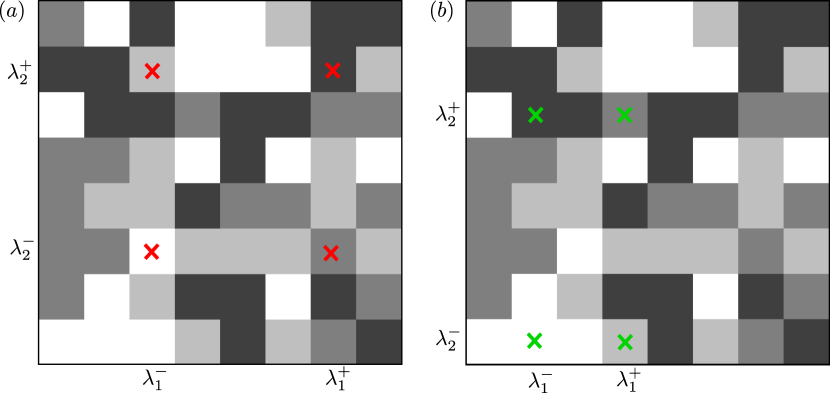
Figure 1: A discrete representation of the basins of attraction, over a phase space of configurations of hidden variables, associated with four measurement outcomes shown as crosses. All the configurations denoted by one of the four shades of grey evolve under measurement towards the appropriately shaded attractor coordinate pair $\left(\lambda_{1}^{\pm},\lambda_{2}^{\pm}\right)$ indicated by a cross $\times$. Situations (a) and (b) correspond to measurement of different system properties with distinct sets (colours) of attractors and associated basins.

The rather abstract discussion given so far can be illustrated using a toy model. Consider a system described by two discrete hidden variables $\lambda_{1,2}$ and a phase space in the form of a grid of squares labelled with integer values. The measurement of properties $A$ and $B$ is represented by attraction of each of $\lambda_{1}$ and $\lambda_{2}$ towards one of two points, yielding four ‘targets’ at coordinates $\left(\lambda_{1}^{\pm},\lambda_{2}^{\pm}\right)$. The idea is that interactions between the system and measuring device bring about a dynamical evolution of the $\lambda_{1,2}$ to attractors (here fixed points) located at the targets. The outcome of the measurement of each property is $\pm$1, as designated by the superscripts on the target coordinates.

We consider a particular situation where passage to each target arises from separate basins of attraction, shown as four different shades of grey. For example, in Figure 1(a) the measurement dynamics generate trajectories starting from any of the black squares and all terminating at $(\lambda_{1}^{+},\lambda_{2}^{+})$.

If there were information on the probabilities of adopting each black square prior to measurement, then we would reasonably deduce from the dynamics that these would accumulate to provide a probability $P_{++}$ of an outcome $A=B=+1$ associated with system arrival at the $(\lambda_{1}^{+},\lambda_{2}^{+})$ target. The suffixes in this probability correspond to the superscripts on the target coordinates. However, we instead wish to deduce the probabilities of having started out on a black square conditioned on information about the type of measurement performed and its outcome. Given that the probability of arrival at $(\lambda_{1}^{+},\lambda_{2}^{+})$ after measurement is $P_{++}$, we need to distribute this probability appropriately over the basin of attraction of that target at earlier times, in accordance with the measurement dynamics. The probability distribution in the past is conditioned on future information: this is the measurement dependence under consideration.

We can now see how such conditioned probabilities would change if the measurement concerned a different property, represented in the toy model as attraction towards a different set of targets. Consider the shifted targets represented by the green crosses in Figure 1(b). The basins of attraction under the measurement dynamics would, in general, form a different pattern for these targets. There are therefore revised probabilities of adoption of configurations prior to measurement when conditioned on a measurement process defined by the green crosses. This is compounded if we consider sets of probabilities of arrival $P_{\pm\pm}$ (outcome probabilities) at the green and red targets that differ from one another.

It is crucial for the emergence of measurement dependence in this toy model that the phase space should separate into a set of basins of attraction to each outcome target for each measurement situation. In real systems where the evolution is deterministic, outcomes are encoded in the coordinates describing the initial state and such a situation would be natural. For systems governed by effective stochastic dynamics arising from coupling to an uncertain environment, such encoding could persist to some degree depending on the situation.

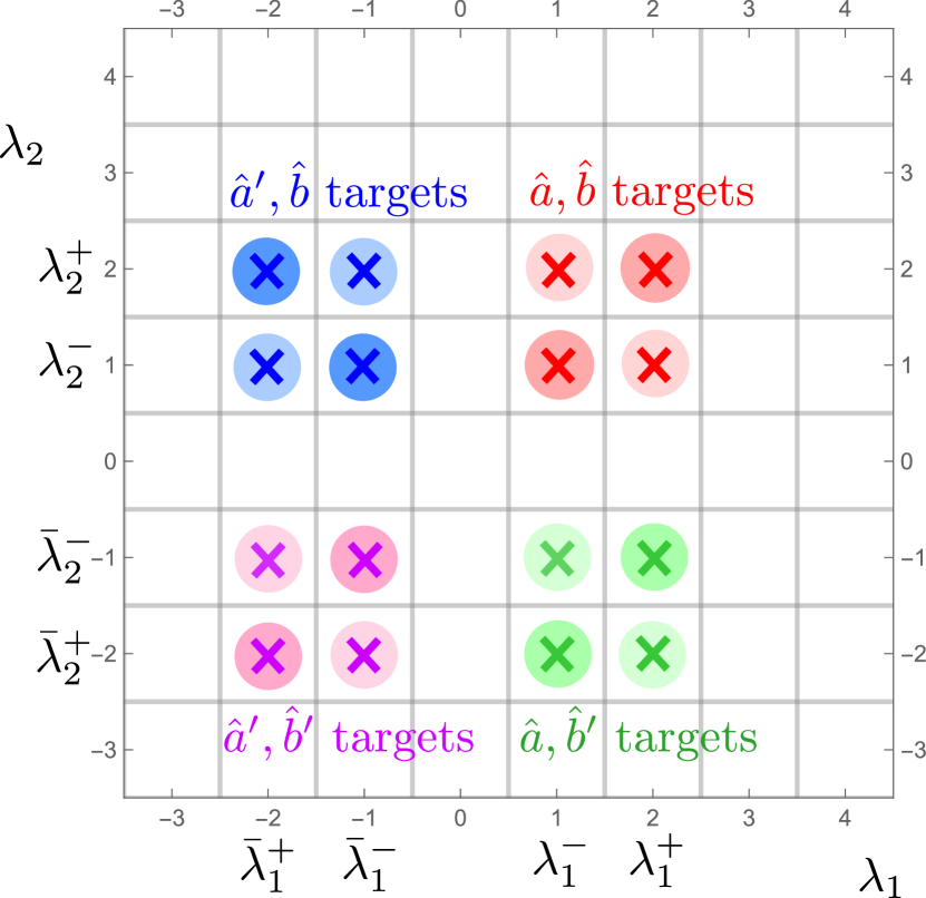
Figure 2: Configurations of the toy model are represented by grid squares in a two dimensional discrete phase space with integer coordinates $\lambda_{1}$ and $\lambda_{2}$. Measurement dynamics draws the configuration towards one of four targets, shown as crosses in a specific colour, representing the four outcomes of measurement of properties $A$ and $B$. Four different experimental circumstances are designated by labels $\hat{a},\hat{b}$, etc, and distinguished by different colours. Arrival at one of the targets yields an outcome $A=\pm 1$ and $B=\pm 1$ according to the superscripts of the $\lambda_{1}$ and $\lambda_{2}$ target coordinates, and the probability of such an outcome is indicated by coloured circles at the targets. The darker the shade, the higher the probability $P_{\pm\pm}^{\hat{x},\hat{y}}$ of arrival at that target.

We now illustrate how a CHSH parameter greater than 2 can be accommodated through this measurement dependence. In Figure 2 we define four sets of targets based on the pairs of positions towards which the measurement dynamics drive the variables $\lambda_{1,2}$. The target pairs $\lambda_{1}^{\pm}$ and $\bar{\lambda}_{1}^{\pm}$ will be labelled ‘axis choices’ $\hat{a}$ and $\hat{a}^{\prime}$, respectively, and $\lambda_{2}^{\pm}$ and $\bar{\lambda}_{2}^{\pm}$ are to be associated with ‘axes’ $\hat{b}$ and $\hat{b}^{\prime}$.The terminology is chosen to establish an analogy with spin component measurement and the superscripts indicate the outcome values for properties $A$and $B$. Four measurement situations can then be considered, specified by the choice of blue, red, purple or green targets. The possible measurement outcomes of $A$ and $B$ can be correlated $(\pm 1,\pm 1)$ or anti-correlated ($\pm 1,\mp 1)$. In Figure 2 we associate +1 outcomes with targets situated at even label positions on the grid and $-1$ outcomes with odd labels.

We can then consider a set of probabilities $P_{\pm\pm}^{\hat{x},\hat{y}}$ for arrival of the system after measurement at the four targets in each group, for $\hat{x}=\hat{a}$ or $\hat{a}^{\prime}$ and $\hat{y}=\hat{b}$ or $\hat{b}^{\prime}$. These are shown in Figure 2 as circular symbols with different shades of colour to indicate magnitude. To simplify the situation, we impose conditions $P_{++}^{\hat{x},\hat{y}}=P_{--}^{\hat{x},\hat{y}}$ and $P_{+-}^{\hat{x},\hat{y}}=P_{-+}^{\hat{x},\hat{y}}$. Furthermore, we consider identical outcome probabilities for the red, blue and purple measurement situations, namely $P_{\pm\pm}^{\hat{a},\hat{b}}=P_{\pm\pm}^{\hat{a}^{\prime},\hat{b}}=P_{\pm\pm}^{\hat{a}^{\prime},\hat{b}^{\prime}}$. However, we design the green measurement situation to be different by setting $P_{\pm\mp}^{\hat{a},\hat{b}^{\prime}}=P_{\pm\pm}^{\hat{a},\hat{b}}$, namely that dark and light shades of green characterise measurement outcomes coloured in light and dark shades, respectively, for the other three cases.We can then combine this information with a chosen pattern of basins of attraction associated with each target to derive the conditioned probabilities over the phase space prior to measurement for each pair of chosen ‘axes’. Our aim is to produce a probability distribution $P(\lambda_{1,2}|\hat{a},\hat{b}^{\prime})$ over the phase space conditioned on outcomes at the green targets that differs from those conditioned on the blue, red and purple targets, which for simplicity we shall choose to be the same, namely $P(\lambda_{1,2}|\hat{a},\hat{b})=P(\lambda_{1,2}|\hat{a}^{\prime},\hat{b})=P(\lambda_{1,2}|\hat{a}^{\prime},\hat{b}^{\prime})\neq P(\lambda_{1,2}|\hat{a},\hat{b}^{\prime})$.The prior distribution over the hidden variables $\lambda_{1,2}$ then clearly depends on the measurement situation. For the green measurement situation, there would be a higher probability associated with the anti-correlated measurement outcomes, whereas correlated outcomes would be more probable if any of the other three measurement situations were considered.

Notice that our approach is to start with the correlation functions for each measurement situation and then to deduce the conditioned probability distributions on the phase space prior to measurement. In this way we can construct a CHSH parameter of any magnitude between zero and 4 but we then need to establish that such a parameter is compatible with an extended upper limit by virtue of the additional term $\mu$ in Eq. (9) arising from differences in the conditioned prior probabilities.

We consider measurement dynamics that generate independent random walks in two dimensions with $|\Delta\lambda_{1}|=|\Delta\lambda_{2}|=2$ per timestep, terminating at a target. We imagine that such a stochastic scheme can emerge from the deterministic dynamics of the system together with a measuring device whose initial state is uncertain. The scheme means that the basin of attraction leading to a target where both $\lambda_{1}$ and $\lambda_{2}$ are even is comprised of all locations in the phase space with similarly even-even coordinates. The basin of attraction leading to a target where $\lambda_{1}$ is even and $\lambda_{2}$ is odd consists of all locations with even-odd coordinates, and so on. Separate basins of attraction to each outcome are maintained. We also assume a phase space with an even number of locations in each dimension ($N$ locations in all) and periodic boundary conditions. This means that the probability $P(\lambda_{1,2}|\hat{a},\hat{b})$ at any even-even location in the phase space, at a sufficiently large interval of time prior to measurement with settings $\hat{a},\hat{b}$, is a constant $P_{ee}^{\hat{a},\hat{b}}$ given by the probability of arrival $P_{++}^{\hat{a},\hat{b}}$ at red target $(\lambda_{1}^{+},\lambda_{2}^{+})$ divided by the number of such locations, $N/4$, which is $P_{ee}^{\hat{a},\hat{b}}=4P_{++}^{\hat{a},\hat{b}}/N$. Similarly, the conditioned probability $P_{eo}^{\hat{a},\hat{b}}$ at an even-odd location on the grid at such a time prior to measurement is the arrival probability $P_{+-}^{\hat{a},\hat{b}}$ at red target $(\lambda_{1}^{+},\lambda_{2}^{-})$ divided equally between all even-odd locations in the grid, or $P_{eo}^{\hat{a},\hat{b}}=4P_{+-}^{\hat{a},\hat{b}}/N$. The conditioned probability at an odd-even location is $P_{oe}^{\hat{a},\hat{b}}=4P_{-+}^{\hat{a},\hat{b}}/N$ and for odd-odd locations it is $P_{oo}^{\hat{a},\hat{b}}=4P_{--}^{\hat{a},\hat{b}}/N$. The same arguments apply to measurement situation $\hat{a},\hat{b}^{\prime}$ with arrival probabilities $P_{\pm\pm}^{\hat{a},\hat{b}^{\prime}}$ at green targets, measurement situation $\hat{a}^{\prime},\hat{b}$ with arrival probabilities $P_{\pm\pm}^{\hat{a}^{\prime},\hat{b}}$ at blue targets, and measurement situation $\hat{a}^{\prime},\hat{b}^{\prime}$ with arrival probabilities $P_{\pm\pm}^{\hat{a}^{\prime},\hat{b}^{\prime}}$ at purple targets.

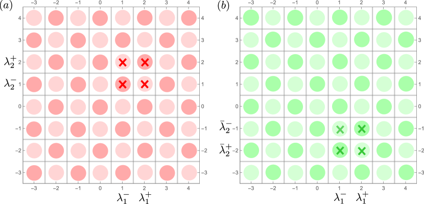
Figure 3: Probability distributions characterising the adoption of toy model configurations prior to measurement of property $AB$ in experimental circumstances (a) $\hat{a},\hat{b}$ and (b) $\hat{a},\hat{b}^{\prime}$, shown on the left and right in pink and green, respectively, with the shades representing magnitude. These are conditioned on (i) the locations of the targets in the grid, to which the configurations are attracted by measurement dynamics consisting of independent symmetric random walks in $\lambda_{1}$ and $\lambda_{2}$ with a step length of 2, and (ii) on the overall probabilities of reaching each of the targets. Notice that the two conditioned probability distributions differ, which is measurement dependence.

What this means is that the conditioned probabilities on the phase space are repeated versions of the patterns of probabilities of arrival at the targets after measurement. This is illustrated in Figure 3(a) for the $\hat{a},\hat{b}$ measurement situation. The dark and light shades of pink represent the two probabilities $P_{ee}^{\hat{a},\hat{b}}$ and $P_{eo}^{\hat{a},\hat{b}}$, respectively, recalling that we have imposed $P_{ee}^{\hat{a},\hat{b}}=P_{oo}^{\hat{a},\hat{b}}$ and $P_{eo}^{\hat{a},\hat{b}}=P_{oe}^{\hat{a},\hat{b}}$. The distribution $P(\lambda_{1,2}|\hat{a},\hat{b})$ illustrated is the discrete analogue of the pdf $\rho(\lambda|\hat{a},\hat{b})$ considered for the spin measurement situation. With the assumptions we have made, the conditioned probability distributions for measurement situations $\hat{a}^{\prime},\hat{b}$ and $\hat{a}^{\prime},\hat{b}^{\prime}$ are identical to the distribution shown for $\hat{a},\hat{b}$ (but would be illustrated in blue and purple, respectively). However, the conditioned probability distribution for the situation $\hat{a},\hat{b}^{\prime}$ shown in Figure 3(b) is different, with a light shade of green, representing $P_{ee}^{\hat{a},\hat{b}^{\prime}}=P_{eo}^{\hat{a},\hat{b}}$, at a location where a dark shade of pink, representing $P_{ee}^{\hat{a},\hat{b}}$, lies in Figure 3(a), and vice versa.

The analogue of the additional term in Eq. (9) for the toy model is a sum of magnitudes of differences between the probability distribution shown in pink in Figure 3(a) and its blue, purple and green counterparts, analogous to $\rho(\lambda|\hat{a},\hat{b})$, $\rho(\lambda|\hat{a}^{\prime},\hat{b})$, $\rho(\lambda|\hat{a}^{\prime},\hat{b}^{\prime})$ and $\rho(\lambda|\hat{a},\hat{b}^{\prime})$, respectively. For the simplified case under consideration, the first three distributions are identical and the fourth is different. This implies, in the notation of a continuum phase space, that $\bar{\rho}\epsilon=-\bar{\rho}\sigma=\bar{\rho}\eta=\frac{1}{4}\left(\rho(\lambda|\hat{a},\hat{b})-\rho(\lambda|\hat{a},\hat{b}^{\prime})\right)$ and hence the additional term in the Bell inequality for $S$ in these circumstances is $\mu=\frac{3}{2}\int|\rho(\lambda|\hat{a},\hat{b})-\rho(\lambda|\hat{a},\hat{b}^{\prime})|d\lambda$.

For the discrete phase space the integral is replaced by a sum of moduli of the differences in probability at each position of the grid conditioned on the red and green measurement outcomes. For the situation we have constructed, these differences are $P_{ee}^{\hat{a},\hat{b}}-P_{ee}^{\hat{a},\hat{b}^{\prime}}$ at even-even and odd-odd points on the grid, and $P_{eo}^{\hat{a},\hat{b}}-P_{eo}^{\hat{a},\hat{b}^{\prime}}$ at even-odd and odd-even points, and these quantities are given by $\pm\left(P_{ee}^{\hat{a},\hat{b}}-P_{eo}^{\hat{a},\hat{b}}\right)$, respectively. The sum of moduli of probability differences over the grid is therefore $N\left|P_{ee}^{\hat{a},\hat{b}}-P_{eo}^{\hat{a},\hat{b}}\right|=4\left|P_{++}^{\hat{a},\hat{b}}-P_{+-}^{\hat{a},\hat{b}}\right|$ and the additional term for the toy model is $\mu=6\left|P_{++}^{\hat{a},\hat{b}}-P_{+-}^{\hat{a},\hat{b}}\right|$.

Similarly, all four correlation functions can be specified in terms of $P_{++}^{\hat{a},\hat{b}}$ and $P_{+-}^{\hat{a},\hat{b}}$, specifically $C(\hat{a},\hat{b})=C(\hat{a}^{\prime},\hat{b})=C(\hat{a}^{\prime},\hat{b}^{\prime})=-C(\hat{a},\hat{b}^{\prime})=2\left(P_{++}^{\hat{a},\hat{b}}-P_{+-}^{\hat{a},\hat{b}}\right)$. Thus the CHSH parameter is $S=4|C(\hat{a},\hat{b})|$ and the additional term is $\mu=3|C(\hat{a},\hat{b})|$. Bell’s analysis therefore requires that

$$S=4|C(\hat{a},\hat{b})|\leq 2+\mu=2+3|C(\hat{a},\hat{b})|,$$ (10)

which is clearly satisfied for the relevant range $0\leq|C(\hat{a},\hat{b})|\leq 1$. We conclude that measurement dependence has elevated the upper limit to accommodate an imposed value of the CHSH parameter.

A toy model can merely illustrate a possibility of behaviour in more realistic systems. It can focus attention on the elements required to be present in those systems to produce an effect. Thus, for example, we see the need for a dynamics of measurement that does not draw configurations towards measurement outcome targets indiscriminately, but instead selects them from basins of attraction in the phase space of hidden variables. We also speculate that a measurement outcome should be associated with system adoption, post-measurement, of a narrowly defined set of hidden variable configurations. The measurement dependence effect might therefore be delicate, and could perhaps emerge only in situations involving few degrees of freedom. The lack of Bell-violating correlations in more complex experimental circumstances might be explained in this way.

The freedom of choice of measurement settings often arises in discussions of measurement dependence. Rather than deny this freedom, a view can be taken that the settings are indeed under experimental control, or can be made effectively random by coupling them to complex external systems. We reiterate that our interest lies in the extent to which the given measurement settings and outcomes can provide information about the subjectively uncertain configuration of system hidden variables prior to measurement. The claim of measurement independence is that no such information is conveyed. But if quantum measurement involves the evolution of hidden variables with measurement settings and outcomes acting as boundary conditions on the dynamics, then conditioning of the probabilities of adopting pre-measurement configurations will follow. This conditioning, or dynamically imposed memory, could extend far back in time, challenging the premise normally employed in the Bell analysis. Perhaps this is the principal implication of the experimental violation of Bell inequalities.

SMW is supported by a PhD studentship funded by EPSRC under grant codes EP/R513143/1 and EP/T517793/1.

References

- Bell [1964] J. S. Bell, On the Einstein-Podolsky-Rosen paradox, Physics 1, 195 (1964).
- Aspect et al. [1982] A. Aspect, J. Dalibard, and G. Roger, Experimental Test of Bell’s Inequalities Using Time-Varying Analyzers, Physical Review Letters 49, 1804 (1982).
- Giustina et al. [2015] M. Giustina, M. A. M. Versteegh, S. Wengerowsky, J. Handsteiner, A. Hochrainer, K. Phelan, F. Steinlechner, J. Kofler, J.-Å. Larsson, C. Abellán, W. Amaya, V. Pruneri, M. W. Mitchell, J. Beyer, T. Gerrits, A. E. Lita, L. K. Shalm, S. W. Nam, T. Scheidl, R. Ursin, B. Wittmann, and A. Zeilinger, Significant-Loophole-Free Test of Bell’s Theorem with Entangled Photons, Physical Review Letters 115, 250401 (2015).
- Christensen et al. [2013] B. G. Christensen, K. T. McCusker, J. B. Altepeter, B. Calkins, T. Gerrits, A. E. Lita, A. Miller, L. K. Shalm, Y. Zhang, S. W. Nam, N. Brunner, C. C. W. Lim, N. Gisin, and P. G. Kwiat, Detection-Loophole-Free Test of Quantum Nonlocality, and Applications, Physical Review Letters 111, 130406 (2013).
- Hensen et al. [2015] B. Hensen, H. Bernien, A. E. Dréau, A. Reiserer, N. Kalb, M. S. Blok, J. Ruitenberg, R. F. L. Vermeulen, R. N. Schouten, C. Abellán, W. Amaya, V. Pruneri, M. W. Mitchell, M. Markham, D. J. Twitchen, D. Elkouss, S. Wehner, T. H. Taminiau, and R. Hanson, Loophole-free Bell inequality violation using electron spins separated by 1.3 kilometres, Nature 526, 682 (2015).
- Shalm et al. [2015] L. K. Shalm, E. Meyer-Scott, B. G. Christensen, P. Bierhorst, M. A. Wayne, M. J. Stevens, T. Gerrits, S. Glancy, D. R. Hamel, M. S. Allman, K. J. Coakley, S. D. Dyer, C. Hodge, A. E. Lita, V. B. Verma, C. Lambrocco, E. Tortorici, A. L. Migdall, Y. Zhang, D. R. Kumor, W. H. Farr, F. Marsili, M. D. Shaw, J. A. Stern, C. Abellán, W. Amaya, V. Pruneri, T. Jennewein, M. W. Mitchell, P. G. Kwiat, J. C. Bienfang, R. P. Mirin, E. Knill, and S. W. Nam, Strong Loophole-Free Test of Local Realism, Physical Review Letters 115, 250402 (2015).
- Rowe et al. [2001] M. A. Rowe, D. Kielpinski, V. Meyer, C. A. Sackett, W. M. Itano, C. Monroe, and D. J. Wineland, Experimental violation of a Bell’s inequality with efficient detection, Nature 409, 791 (2001).
- Bell [2004] J. S. Bell, Speakable and Unspeakable in Quantum Mechanics: Collected Papers on Quantum Philosophy, 2nd ed. (Cambridge University Press, Cambridge, 2004).
- Norsen [2017] T. Norsen, Foundations of Quantum Mechanics: An Exploration of the Physical Meaning of Quantum Theory (Springer, Cham, Switzerland, 2017).
- Hossenfelder and Palmer [2020] S. Hossenfelder and T. Palmer, Rethinking superdeterminism, Frontiers in Physics 8, 139 (2020).
- Clauser et al. [1969] J. F. Clauser, M. A. Horne, A. Shimony, and R. A. Holt, Proposed experiment to test local hidden-variable theories, Physical Review Letters 23, 880 (1969).
- Wharton and Argaman [2020] K. B. Wharton and N. Argaman, Colloquium: Bell’s theorem and locally mediated reformulations of quantum mechanics, Reviews of Modern Physics 92, 021002 (2020).
- Pütz and Gisin [2016] G. Pütz and N. Gisin, Measurement dependent locality, New Journal of Physics 18, 055006 (2016).
- Friedman et al. [2019] A. S. Friedman, A. H. Guth, M. J. W. Hall, D. I. Kaiser, and J. Gallicchio, Relaxed Bell inequalities with arbitrary measurement dependence for each observer, Physical Review A 99, 012121 (2019).
- Toner and Bacon [2003] B. F. Toner and D. Bacon, Communication Cost of Simulating Bell Correlations, Physical Review Letters 91, 187904 (2003).
- Hall and Branciard [2020] M. J. W. Hall and C. Branciard, Measurement-dependence cost for Bell nonlocality: Causal versus retrocausal models, Physical Review A 102, 052228 (2020).
- Brans [1988] C. H. Brans, Bell’s theorem does not eliminate fully causal hidden variables, International Journal of Theoretical Physics 27, 219 (1988).
- Banik et al. [2012] M. Banik, M. R. Gazi, S. Das, A. Rai, and S. Kunkri, Optimal free will on one side in reproducing the singlet correlation, Journal of Physics A: Mathematical and Theoretical 45, 205301 (2012).
- Sadhu and Das [2023] A. Sadhu and S. Das, Testing of quantum nonlocal correlations under constrained free will and imperfect detectors, Physical Review A 107, 012212 (2023).
- Chaves et al. [2021] R. Chaves, G. Moreno, E. Polino, D. Poderini, I. Agresti, A. Suprano, M. R. Barros, G. Carvacho, E. Wolfe, A. Canabarro, R. W. Spekkens, and F. Sciarrino, Causal Networks and Freedom of Choice in Bell’s Theorem, PRX Quantum 2, 040323 (2021).
- Acín and Masanes [2016] A. Acín and L. Masanes, Certified randomness in quantum physics, Nature 540, 213 (2016).
- Bierhorst et al. [2018] P. Bierhorst, E. Knill, S. Glancy, Y. Zhang, A. Mink, S. Jordan, A. Rommal, Y.-K. Liu, B. Christensen, S. W. Nam, M. J. Stevens, and L. K. Shalm, Experimentally generated randomness certified by the impossibility of superluminal signals, Nature 556, 223 (2018).
- Colbeck and Renner [2012] R. Colbeck and R. Renner, Free randomness can be amplified, Nature Physics 8, 450 (2012).
- Kessler and Arnon-Friedman [2020] M. Kessler and R. Arnon-Friedman, Device-Independent Randomness Amplification and Privatization, IEEE Journal on Selected Areas in Information Theory 1, 568 (2020).
- Koh et al. [2012] D. E. Koh, M. J. W. Hall, Setiawan, J. E. Pope, C. Marletto, A. Kay, V. Scarani, and A. Ekert, Effects of Reduced Measurement Independence on Bell-Based Randomness Expansion, Physical Review Letters 109, 160404 (2012).
- Liu et al. [2018a] Y. Liu, Q. Zhao, M.-H. Li, J.-Y. Guan, Y. Zhang, B. Bai, W. Zhang, W.-Z. Liu, C. Wu, X. Yuan, H. Li, W. J. Munro, Z. Wang, L. You, J. Zhang, X. Ma, J. Fan, Q. Zhang, and J.-W. Pan, Device-independent quantum random-number generation, Nature 562, 548 (2018a).
- Liu et al. [2018b] Y. Liu, X. Yuan, M.-H. Li, W. Zhang, Q. Zhao, J. Zhong, Y. Cao, Y.-H. Li, L.-K. Chen, H. Li, T. Peng, Y.-A. Chen, C.-Z. Peng, S.-C. Shi, Z. Wang, L. You, X. Ma, J. Fan, Q. Zhang, and J.-W. Pan, High-Speed Device-Independent Quantum Random Number Generation without a Detection Loophole, Physical Review Letters 120, 010503 (2018b).
- Pironio et al. [2010] S. Pironio, A. Acín, S. Massar, A. B. de la Giroday, D. N. Matsukevich, P. Maunz, S. Olmschenk, D. Hayes, L. Luo, T. A. Manning, and C. Monroe, Random numbers certified by Bell’s theorem, Nature 464, 1021 (2010).
- Wooltorton et al. [2022] L. Wooltorton, P. Brown, and R. Colbeck, Tight Analytic Bound on the Trade-Off between Device-Independent Randomness and Nonlocality, Physical Review Letters 129, 150403 (2022).
- Yuan et al. [2015] X. Yuan, Z. Cao, and X. Ma, Randomness requirement on the Clauser-Horne-Shimony-Holt Bell test in the multiple-run scenario, Physical Review A 91, 032111 (2015).
- Gallicchio et al. [2014] J. Gallicchio, A. S. Friedman, and D. I. Kaiser, Testing Bell’s Inequality with Cosmic Photons: Closing the Setting-Independence Loophole, Physical Review Letters 112, 110405 (2014).
- Handsteiner et al. [2017] J. Handsteiner, A. S. Friedman, D. Rauch, J. Gallicchio, B. Liu, H. Hosp, J. Kofler, D. Bricher, M. Fink, C. Leung, A. Mark, H. T. Nguyen, I. Sanders, F. Steinlechner, R. Ursin, S. Wengerowsky, A. H. Guth, D. I. Kaiser, T. Scheidl, and A. Zeilinger, Cosmic Bell Test: Measurement Settings from Milky Way Stars, Physical Review Letters 118, 060401 (2017).
- Rauch et al. [2018] D. Rauch, J. Handsteiner, A. Hochrainer, J. Gallicchio, A. S. Friedman, C. Leung, B. Liu, L. Bulla, S. Ecker, F. Steinlechner, R. Ursin, B. Hu, D. Leon, C. Benn, A. Ghedina, M. Cecconi, A. H. Guth, D. I. Kaiser, T. Scheidl, and A. Zeilinger, Cosmic Bell Test Using Random Measurement Settings from High-Redshift Quasars, Physical Review Letters 121, 080403 (2018).
- Wu et al. [2017] C. Wu, B. Bai, Y. Liu, X. Zhang, M. Yang, Y. Cao, J. Wang, S. Zhang, H. Zhou, X. Shi, X. Ma, J.-G. Ren, J. Zhang, C.-Z. Peng, J. Fan, Q. Zhang, and J.-W. Pan, Random Number Generation with Cosmic Photons, Physical Review Letters 118, 140402 (2017).
- Li et al. [2018] M.-H. Li, C. Wu, Y. Zhang, W.-Z. Liu, B. Bai, Y. Liu, W. Zhang, Q. Zhao, H. Li, Z. Wang, L. You, W. J. Munro, J. Yin, J. Zhang, C.-Z. Peng, X. Ma, Q. Zhang, J. Fan, and J.-W. Pan, Test of Local Realism into the Past without Detection and Locality Loopholes, Physical Review Letters 121, 080404 (2018).
- Das et al. [2021] S. Das, S. Bäuml, M. Winczewski, and K. Horodecki, Universal Limitations on Quantum Key Distribution over a Network, Physical Review X 11, 041016 (2021).
- Ekert [1991] A. K. Ekert, Quantum cryptography based on Bell’s theorem, Physical Review Letters 67, 661 (1991).
- Holz et al. [2020] T. Holz, H. Kampermann, and D. Bruß, Genuine multipartite Bell inequality for device-independent conference key agreement, Physical Review Research 2, 023251 (2020).
- Horodecki et al. [2022] K. Horodecki, M. Winczewski, and S. Das, Fundamental limitations on the device-independent quantum conference key agreement, Physical Review A 105, 022604 (2022).
- Kaur et al. [2022] E. Kaur, K. Horodecki, and S. Das, Upper Bounds on Device-Independent Quantum Key Distribution Rates in Static and Dynamic Scenarios, Physical Review Applied 18, 054033 (2022).
- Li et al. [2022] X. Li, Y. Wang, Y. Han, and S.-N. Zhu, Effects of reduced measurements independence on self-testing, Journal of Physics A: Mathematical and Theoretical 55, 495302 (2022).
- Moroder et al. [2013] T. Moroder, J.-D. Bancal, Y.-C. Liang, M. Hofmann, and O. Gühne, Device-Independent Entanglement Quantification and Related Applications, Physical Review Letters 111, 030501 (2013).
- Primaatmaja et al. [2023] I. W. Primaatmaja, K. T. Goh, E. Y.-Z. Tan, J. T.-F. Khoo, S. Ghorai, and C. C.-W. Lim, Security of device-independent quantum key distribution protocols: A review, Quantum 7, 932 (2023).
- Vazirani and Vidick [2014] U. Vazirani and T. Vidick, Fully Device-Independent Quantum Key Distribution, Physical Review Letters 113, 140501 (2014).
- Zapatero et al. [2023] V. Zapatero, T. van Leent, R. Arnon-Friedman, W.-Z. Liu, Q. Zhang, H. Weinfurter, and M. Curty, Advances in device-independent quantum key distribution, npj Quantum Information 9, 1 (2023).
- Hall [2010] M. J. W. Hall, Local deterministic model of singlet state correlations based on relaxing measurement independence, Physical Review Letters 105, 250404 (2010).
- Pütz et al. [2014] G. Pütz, D. Rosset, T. J. Barnea, Y.-C. Liang, and N. Gisin, Arbitrarily Small Amount of Measurement Independence Is Sufficient to Manifest Quantum Nonlocality, Physical Review Letters 113, 190402 (2014).
- Šupić et al. [2022] I. Šupić, J.-D. Bancal, and N. Brunner, Quantum nonlocality in presence of strong measurement dependence (2022), arxiv:2209.02337 [quant-ph] .
- Kim et al. [2019] M. Kim, J. Lee, H.-J. Kim, and S. W. Kim, Tightest conditions for violating the Bell inequality when measurement independence is relaxed, Physical Review A 100, 022128 (2019).