The Haldane Model in a Magneto-optical Honeycomb Lattice

Abstract

A two-dimensional honeycomb lattice composed of gyrotropic rods is studied. Beginning with Maxwell’s equations, a perturbed Wannier method is introduced which yields a tight-binding model with nearest and next-nearest neighbors. The resulting discrete model leads to a Haldane model and as such, topologically protected modes, associated with nonzero Chern numbers are supported. Changing the radii of the rods allows for the breaking of inversion symmetry which can change the topology of the system. This model explains experimental results associated with topological waves in magneto-optical honeycomb lattices. This method can also be applied to more general Chern insulator lattices. When on-site Kerr type nonlinear effects are considered, coherent soliton-like modes are found to propagate robustly through boundary defects.

I Introduction

The study of topological insulators is an area of research currently receiving significant interest. These types of systems can be experimentally realized in numerous fields including ultracold fermionic systems Jotzu2014 , semiconductors vonKlitzing1980 ; Bernevig2006 , magnetic media Chang2013 , equatorial waves Delplace2017 , and electromagnetic systems Rechtsman2013 ; Ozawa2019 ; Lu2014 . Underlying these works are topologically protected states that are robust to defects.

This work focuses on topological insulators that are distinguished by bulk eigenmodes with a nontrivial Chern number. In this case, the bulk-edge correspondence implies the existence of topologically protected modes. Indeed, these systems can support edge states that propagate unidirectionally around the boundary with and without material defects.

A standard approach for describing topological insulator lattice systems is the use of a tight-binding model. Typically, tight-binding models consist of a set of discrete equations that reduce the complexity of the governing equations, yet still capture the essential behavior. Moreover, it is common in experiments for the dielectric contrast in photonic waveguides to naturally reside in the deep lattice regime which is central in the tight-binding approximation Ablowitz2022a ; Fefferman2018 .

One of the most well-known and heavily studied topological insulator systems is the Haldane model Haldane1988 , associated with honeycomb lattices. This relatively simple model, which includes nearest and next-nearest neighbor interactions, is able to capture the essence of Chern insulator systems. The model illustrates that breaking of time-reversal symmetry is necessary, but not sufficient, for realizing bulk modes with nontrivial Chern topological invariants. Moreover, when inversion symmetry is broken in an appropriate manner exceeding that of time-reversal symmetry, a topological transition to a trivial Chern system can take place.

While Haldane1988 offers no derivation for the model, it effectively describes the behavior of the quantum Hall effect in honeycomb lattices. Indeed, many authors have applied the Haldane model to describe systems with nonzero Chern numbers. However, it is not clear whether this is the true tight-binding reduction of electromagnetic systems or just a convenient model.

This work provides a direct derivation of the Haldane model from Maxwell’s equations in a magneto-optical (MO) system. The physical system considered here is that of transverse magnetic (TM) waves in a ferrimagnetic photonic crystal with an applied external magnetic field. Systems of this type have been realized in both square Wang2008 ; Wang2009 ; Sun2019 ; Yang2013 and honeycomb Ao2009 ; Poo2011 ; Zhao2020 lattices and found to support topologically protected edge modes. Topologically protected modes in EM systems were originally proposed by Haldane and Raghu Haldane2008 ; Raghu2008 and their existence studied in LeeThorp2019 . Our work directly connects Haldane’s model Haldane1988 to electro-magneto-optical systems. Additionally, it turns out that periodically driven photonic honeycomb lattices can also yield the Haldane model in a high-frequency limit Jotzu2014 ; Ablowitz2022 .

The key to our approach is to use a suitable Wannier basis in which to expand the EM field Ablowitz2020 . Unfortunately, a direct Wannier expansion is ineffective due to nontrivial topology which is the result of a discontinuity in the spectral phase of the associated Bloch function Brouder2007 ; Ablowitz2022 . As a result, the corresponding Wannier-Fourier coefficients do not decay rapidly. Seeking a tight-binding model in a basis of these slowly decaying Wannier modes would require many interactions, well beyond nearest neighbor, to accurately describe the problem. Consequently, this would cease to be an effective reduction of the original problem.

By considering nearest and next-nearest neighbor interactions, a Haldane model is derived from the original MO honeycomb lattice. With physically relevant parameters, an analytical study of the system topology is conducted. The topological transition points are identified and found to agree well with numerical approximations. Nontrivial Chern numbers are found to correspond to unidirectional chiral modes, and vice versa for trivial Chern cases.

The Wannier basis method we use was applied to a square MO lattice in Ablowitz2020 . The results in this paper show that the method is effective, again. This approach can be applied to other systems, e.g. different lattices, governed by the TM equation with gyrotropic lattices. We expect this method to model other Chern insulator systems, e.g. TE systems with gyrotropic permittivity, as well.

We also examine the effect of nonlinearity on edge mode propagation. Edge solitons, unidirectional nonlinear envelopes that balance nonlinearity and dispersion have been explored in Floquet Chern insulator systems Ablowitz2014 ; Ablowitz2017 . The work Mukherjee2021 showed that significant amounts of radiation are emitted from the solitary wave for highly localized (nonlinear) envelopes.

The nonlinear system we consider is a Haldane model that includes on-site Kerr nonlinearity. A similar system has also been derived from nonlinear a Floquet system in a high-frequency driving limit Ablowitz2022 . Different nonlinear Haldane models with saturable nonlinearity Harari2018 and mass terms Zhou2017 have previously been explored. Using balanced envelopes such as those described above as a guide, we observe that slowly-varying envelopes can propagate coherently and robustly around lattice boundaries. Due to their ability to balance nonlinear and dispersive effects, while localized along the boundary, we call these edge solitons.

II Magneto-optical System

The setup we consider is a planar array ${\bf r}=(x,y)^{T}$ of ferrimagnetic rods, e.g. YIG rods, arranged in a honeycomb lattice pattern (see Fig. 1). Similar designs were implemented in Wang2008 ; Wang2009 and Ao2009 ; Poo2011 . The parallelogram unit cell contains an “a-site” and “b-site” with radii of $R_{a}$ and $R_{b}$, respectively. All other cells are integer translations of the lattice vectors

$${\bf v}_{1}=\ell\begin{pmatrix}\frac{3}{2}\\ \frac{\sqrt{3}}{2}\end{pmatrix},~{}~{}~{}{\bf v}_{2}=\ell\begin{pmatrix}\frac{3}{2}\\ -\frac{\sqrt{3}}{2}\end{pmatrix}$$

from the unit cell, where $\ell$ is the distance between nearest neighbor rods. The notation $(m,n)$ indicates a rod that is displaced $m{\bf v}_{1}+n{\bf v}_{2}$ away from the unit cell, where $m,n\in\mathbb{Z}.$

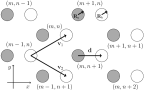
Figure 1: Planar honeycomb array of ferrite rods. The lattice a-sites (b-sites) are grey (white) discs with radius $R_{a}$ ($R_{b}$). A constant magnetic field $H_{0}\widehat{{\bf z}}$ is applied. The indices $(m,n)$ denote integer shifts in the ${\bf v}_{1}$ and ${\bf v}_{2}$ directions, respectively. The displacement between two rods in the same cell is ${\bf d}$ with $||{\bf d}||_{2}=\ell$.

A constant external magnetic field is applied in the perpendicular (out of the page) direction: $H_{0}\widehat{\bf z}$, and saturated magnetization. For time-harmonic fields with angular frequency $\omega$, the ferrite rods induce the gyrotropic permeability tensor Pozar

$$[\mu]=\begin{pmatrix}\mu&i\kappa&0\\ -i\kappa&\mu&0\\ 0&0&\mu_{0}\end{pmatrix},$$

where $\mu=\mu_{0}\left(1+\frac{\omega_{0}\omega_{m}}{\omega_{0}^{2}-\omega^{2}}\right)$ and $\kappa=\mu_{0}\frac{\omega\omega_{m}}{\omega_{0}^{2}-\omega^{2}}$. The coefficients are defined in terms of $\omega_{0}=\mu_{0}\gamma H_{0}$ and $\omega_{m}=\mu_{0}\gamma M_{s}$, where $\mu_{0}$ is the vacuum permeability, $\gamma$ is the gyromagnetic ratio, and $M_{s}$ is the magnetization saturation of the material.

For rods with permittivity $\varepsilon({\bf r})$, the governing TM wave equation for a time-harmonic field is

$$-\nabla^{2}E+\mathcal{M}\cdot\nabla E=\omega^{2}\varepsilon\tilde{\mu}E,$$

$$\mathcal{M}({\bf r})=\nabla\ln\tilde{\mu}-i\tilde{\mu}(\widehat{{\bf z}}\times\nabla\eta),$$

where $E$, plus its complex conjugate, is the $z$-component of the electric field, $\tilde{\mu}=\frac{\mu^{2}-\kappa^{2}}{\mu}$ and $\eta=-\frac{\kappa}{\mu^{2}-\kappa^{2}}$. Here we take a non-dispersive approximation and fix the values of $\mu$ and $\kappa$: $\omega$ is fixed to eventual band gap frequencies. For a typical YIG rod at frequency $f=7.7$GHz ($f=\omega/2\pi$) with saturation magnetization $4\pi M_{s}=1750$ G and magnetizing field $H_{0}=500$ Oe, the constitutive relations are approximately $\mu=0.88\mu_{0},\kappa=-0.66\mu_{0}$ and $\varepsilon=15\varepsilon_{0}$. The equation is nondimensionalized via: ${\bf r}\rightarrow\ell{\bf r},\mu\rightarrow\mu_{0}\mu,\kappa\rightarrow\mu_{0}\kappa,\varepsilon\rightarrow\varepsilon_{0}\varepsilon,\omega\rightarrow c\omega/\ell$, where $c$ is the speed of light and $\varepsilon_{0}=(c^{2}\mu_{0})^{-1}$ is the vacuum permittivity.

The coefficients in (II) share the translation symmetry of the honeycomb lattice: $\varepsilon({\bf r}+m{\bf v}_{1}+n{\bf v}_{2})=\varepsilon({\bf r}),\tilde{\mu}({\bf r}+m{\bf v}_{1}+n{\bf v}_{2})=\tilde{\mu}({\bf r}),$ and $\eta({\bf r}+m{\bf v}_{1}+n{\bf v}_{2})=\eta({\bf r})$ where $m,n\in\mathbb{Z}$. Bloch theory motivates bulk wave solutions of the form $E({\bf r};{\bf k})=e^{i{\bf k}\cdot{\bf r}}u({\bf r};{\bf k})$, where $u({\bf r}+m{\bf v}_{1}+n{\bf v}_{2};{\bf k})=u({\bf r};{\bf k})$ for quasimomentum ${\bf k}$ where these reciprocal lattice vectors are given by

$${\bf k}_{1}=\frac{2\pi}{\ell}\begin{pmatrix}\frac{1}{3}\\ \ \frac{1}{\sqrt{3}}\end{pmatrix},~{}~{}~{}{\bf k}_{2}=\frac{2\pi}{\ell}\begin{pmatrix}~{}\frac{1}{3}\\ \ -\frac{1}{\sqrt{3}}\end{pmatrix}.$$

Solving the resulting equation for $(u({\bf r};{\bf k}),\omega({\bf k}))$, via spectral methods along the $\Gamma MK\Gamma$ path in ${\bf k}-$space (see Appendix A), we obtain the two lowest spectral bands shown in Fig. 2.

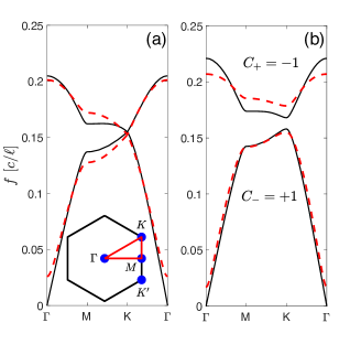
Figure 2: Normalized frequency bands obtained by solving (II) for $u({\bf r};{\bf k})=e^{-i{\bf k}\cdot{\bf r}}E({\bf r};{\bf k})$ along the path $\Gamma MK\Gamma$ with $R_{a}=R_{b}=0.3\ell$. Shown are the first two bands (ascending order) for (a) non-magnetized ($\mathcal{M}={\bf 0},\tilde{\mu}=\mu_{0}$) and (b) magnetized ($\mathcal{M}\not={\bf 0},\tilde{\mu}\not=\mu_{0}$) systems. Solid lines indicate numerically computed curves. Dashed lines denote the tight-binding approximation discussed below.

The location of Dirac points are

$$K^{\prime}=\begin{pmatrix}0\\ \frac{4\pi}{3\sqrt{3}\ell}\end{pmatrix},~{}~{}K=\begin{pmatrix}0\\ -\frac{4\pi}{3\sqrt{3}\ell}\end{pmatrix}.$$

In Fig. 2(a), no external magnetic field is applied and a conical Dirac point is observed at the $K$ point. When a magnetic field is applied, then $\mathcal{M}$ is nonzero, time-reversal symmetry is broken and a band gap opens [see Fig. 2(b)]. Moreover, there is an associated set of nonzero Chern numbers. Note that the first (lowest) band is denoted by ‘–’ subscript, while the second band is denoted by ‘+’ subscript. In Fig. 2 we also compare with the discrete–tight binding approximation discussed below.

III A Perturbed Wannier Approach

A strong dielectric contrast between the rods and background motivates a tight-binding approximation, whereby a variable coefficient PDE with a periodic lattice potential, i.e. (II), can be reduced to a constant coefficient system of ODEs Ablowitz2022a . Bloch wave solutions of (II) are periodic with respect to the quasimomentum ${\bf k}$: $E({\bf r};{\bf k}+m{\bf k}_{1}+n{\bf k}_{2})=E({\bf r};{\bf k})$, where the reciprocal lattice vectors ${\bf k}_{1,2}$ and satisfy ${\bf v}_{i}\cdot{\bf k}_{j}=2\pi\delta_{ij}$. As such, the Bloch wave can be expanded in a Fourier in ${\bf k}$ series

$$E({\bf r};{\bf k})=\sum_{p}\sum_{m,n}W_{mn}^{p}({\bf r})e^{i{\bf k}\cdot(m{\bf v}_{1}+n{\bf v}_{2})},$$ (2)

where $W_{mn}^{p}$ denotes the Wannier function corresponding to the $(m,n)$ spatial cell and $p^{\rm th}$ spectral band.

Due to the properties of Fourier coefficients, the decay of $W_{mn}^{p}({\bf r})$ depends on the smoothness of $E({\bf r};{\bf k})$ in ${\bf k}$. Chern insulators possess an essential phase discontinuity that can not be removed via gauge transformation Brouder2007 . As a result, a direct Wannier expansion is not useful. But, a closely related set of exponentially localized Wannier functions, which come from a problem with time-reversal symmetry Ablowitz2020 can be used perturbatively.

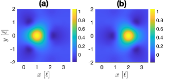
Figure 3: Maximally localized Wannier functions (a) $\widetilde{W}^{a}_{00}({\bf r})$ and (b)$\widetilde{W}^{b}_{00}({\bf r})$, obtained from (II) when $\mathcal{M}={\bf 0}$ and $R_{a}=R_{b}=0.3\ell$.

Consider (II) with $\mathcal{M}={\bf 0}$, but $\tilde{\mu}\not=\mu_{0}$; the so-called “perturbed problem”. The maximally localized Wannier (MLWF) functions, found using well-known methods Marzari1997 , corresponding to the first two Wannier functions, called $\widetilde{W}^{a}_{mn}({\bf r})$ and $\widetilde{W}^{b}_{mn}({\bf r})$, are shown in Fig. 3 and centered at the a-sites (${\bf d}+m{\bf v}_{1}+n{\bf v}_{2}$) and b-sites ($2{\bf d}+m{\bf v}_{1}+n{\bf v}_{2}$), respectively. These Wannier functions are related to those in (2) by a unitary transformation chosen to minimize the variance (see Appendix C). Note that these functions are real, exponentially localized, and approximately possess mirror symmetry about the $x=3\ell/2$ axis; i.e. $\widetilde{W}^{a}_{00}(-({\bf r}-3\ell\widehat{{\bf x}}/2))=\widetilde{W}^{b}_{00}({\bf r}-3\ell\widehat{{\bf x}}/2)$.

The Bloch wave is expanded in terms of this new basis as

$${E}({\bf r};{\bf k}) =\sum_{m,n}(a_{mn}\widetilde{W}^{a}_{mn}({\bf r})+b_{mn}\widetilde{W}^{b}_{mn}({\bf r})),$$ (3)

where the phases have been absorbed into the coefficients. Properly normalized Wannier modes exhibit the orthogonality property $\langle W_{mn}^{p},W_{m^{\prime}n^{\prime}}^{p^{\prime}}\rangle_{\mathbb{R}^{2}}=\delta_{mm^{\prime}}\delta_{nn^{\prime}}\delta_{pp^{\prime}}$ for the weighted complex inner product $\langle f,g\rangle_{\mathbb{R}^{2}}=\iint_{\mathbb{R}^{2}}f({\bf r})^{*}g({\bf r})\varepsilon({\bf r})\tilde{\mu}({\bf r})d{\bf r}$.

Substituting (3) into (II) with $\mathcal{M}\not=0$, multiplying by $\widetilde{W}^{j}_{mn}({\bf r}),j=a,b,$ and integrating over $\mathbb{R}^{2}$ yields a system of algebraic equations whose coefficients depend on integrals over perturbed Wannier functions. Once the MLWFs are obtained, these integrals are numerically approximated. Due to the deep lattice, in the simplest tight-binding approximation only nearby interactions are kept since the others are small. Below we keep terms up to the next-nearest neighboring sites.

IV A Haldane-type Model

Inspection of the numerically computed tight-binding coefficients (see Appendix A) reveals an effective discrete approximation that is essentially the well-known Haldane model Haldane1988 . Namely, replacing $\omega$ by $id/dt$ we obtain

$$\frac{d^{2}a_{mn}}{dt^{2}} +Pa_{mn}+t_{1}(\delta_{-}b_{mn})$$ (4)

$$+t_{2}e^{i\phi}(\Delta_{1}a_{mn})+t_{2}e^{-i\phi}(\Delta_{2}a_{mn})=0$$

$$\frac{d^{2}b_{mn}}{dt^{2}} +\widetilde{P}b_{mn}+t_{1}(\delta_{+}a_{mn})$$ (5)

$$+\tilde{t}_{2}e^{-i{\phi}}(\Delta_{1}b_{mn})+\tilde{t}_{2}e^{i{\phi}}(\Delta_{2}b_{mn})=0$$

where $(\delta_{\pm}c_{mn})\equiv c_{mn}+c_{m\pm 1,n}+c_{m,n\pm 1}$ are the nearest neighbor interactions and $(\Delta_{1}c_{mn})\equiv c_{m,n+1}+c_{m-1,n}+c_{m+1,n-1}$ and $(\Delta_{2}c_{mn})\equiv c_{m+1,n}+c_{m,n-1}+c_{m-1,n+1}$ are next-nearest neighbor contributions; parameters $P,\widetilde{P},t_{1},t_{2},\tilde{t}_{2},\phi$ are real numbers; these values depend on the values of $\mu,\kappa,\varepsilon$ and sizes of the radii of the rods. Notice that this system reduces to the ‘classical’ Haldane model given in Haldane1988 when $\tilde{t}_{2}=t_{2}$ and $\phi\rightarrow-\phi$. The equations can be put in a more standard form by looking for solutions of the form $a_{mn}\rightarrow a_{mn}e^{i\omega t},$ similarly for $b_{mn},$ and then shifting the spectrum $\omega^{2}\rightarrow\omega^{2}+(P+\widetilde{P})/2$. This yields an on-site inversion parameter

$$M\equiv\frac{P-\widetilde{P}}{2}$$ (6)

which is important in Haldane1988 and below. The result of this latter spectral shift is to effectively replace $P$ in (4) by $M$ and $\widetilde{P}$ in (5) by $-M$.

We find the ‘classical’ Haldane model when inversion symmetry is not broken ($P=\widetilde{P},t_{2}=\tilde{t}_{2})$ and a modified version when inversion symmetry is broken ($P\neq\widetilde{P},t_{2}\not=\tilde{t}_{2})$. When the a-site and b-site rods differ, the inversion symmetry of the lattice ${\bf r}\rightarrow-{\bf r}$ is broken and this leads to different interactions among the Wannier modes (see Sec. IV.2 and Appendix C).

The physical derivation that leads to the model (4)-(5) should be pointed out. The external magnetic field induces the complex next-nearest coefficients in the system. Furthermore, this method appears applicable for the derivation of other tight-binding models in Chern insulator systems.

We compare the bulk bands of the discrete model to those numerically computed from (II); see Fig. 2. (All tight-binding parameters used can be found in Appendix B) Indeed, the discrete approximation shows good agreement with the numerical bands; the relative error throughout the Brillouin zone is 6.5% or less. Moreover, for $\ell=5.8$ mm spacing, the gap frequencies in Fig. 2(b) lie in the vicinity of the 8 GHz microwave regime found in Poo2011 .

IV.1 Analytical Calculation of Bulk Modes

Consider bulk plane wave solutions of system (4)-(5) of the form

$$a_{mn}(t) =\alpha({\bf k})e^{i\left[{\bf k}\cdot(m{\bf v}_{1}+n{\bf v}_{2})-\omega({\bf k})t\right]},$$

$$b_{mn}(t) =\beta({\bf k})e^{i\left[{\bf k}\cdot(m{\bf v}_{1}+n{\bf v}_{2})-\omega({\bf k})t\right]},$$

where ${\bf k}\in\mathbb{R}$. Next, define the nearest neighbor and next-nearest neighbor vectors ${\bf a}_{1}={\bf 0},{\bf a}_{2}={\bf v}_{1},{\bf a}_{3}={\bf v}_{2}$, and ${\bf b}_{1}={\bf v}_{1},{\bf b}_{2}=-{\bf v}_{2},{\bf b}_{3}={\bf v}_{2}-{\bf v}_{1},$ respectively. Then the bulk Haldane system can be expressed as the following eigenvalue system

$$\begin{pmatrix}M+H_{0}+H_{3}&H_{1}-iH_{2}\\ H_{1}+iH_{2}&-M+\tau(H_{0}-H_{3})\end{pmatrix}\begin{pmatrix}\alpha\\ \beta\end{pmatrix}=\widetilde{\omega}^{2}\begin{pmatrix}\alpha\\ \beta\end{pmatrix}$$ (7)

where $\tau=\tilde{t}_{2}/t_{2}>0$ and $M=(P-\widetilde{P})/2$ with the terms

$$H_{0}({\bf k}) =2t_{2}\sum_{j=1}^{3}\cos\phi\cos({\bf k}\cdot{\bf b}_{j})$$

$$H_{1}({\bf k}) =t_{1}\sum_{j=1}^{3}\cos({\bf k}\cdot{\bf a}_{j})$$

$$H_{2}({\bf k}) =t_{1}\sum_{j=1}^{3}\sin({\bf k}\cdot{\bf a}_{j})$$

$$H_{3}({\bf k}) =2t_{2}\sum_{j=1}^{3}\sin\phi\sin({\bf k}\cdot{\bf b}_{j}).$$

Note that we have utilized the frequency shift $\omega^{2}=\widetilde{\omega}^{2}+(P+\widetilde{P})/2$ to follow the convention used in Haldane1988 . When $\tau=1$ this is precisely Haldane’s model Haldane1988 when $\phi\rightarrow-\phi$ and $\widetilde{\omega}^{2}\rightarrow\overline{\omega}^{2}+H_{0}$. The dispersion surfaces of (7) are given by

$$\widetilde{\omega}^{2}_{\pm}({\bf k})=\frac{H_{0}({\bf k})(1+\tau)+H_{3}({\bf k})(1-\tau)}{2}\pm\sqrt{H_{1}({\bf k})^{2}+H_{2}({\bf k})^{2}+\frac{1}{4}\left[2M+H_{0}({\bf k})(1-\tau)+H_{3}({\bf k})(1+\tau)\right]^{2}}.$$ (8)

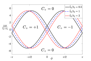
Figure 4: Phase diagram separating nontrivial Chern insulator (interior) and trivial system (exterior) for different ratios of $\tilde{t}_{2}/t_{2}.$ Shown is the Chern number $C_{+}$ for the second spectral band; the signs are reversed for $C_{-}$ corresponding to the first band. Note: $\tau=\tilde{t}_{2}/t_{2}$ is a function of $R_{a}/R_{b}$.

Below, we begin by studying the behavior of the spectrum near the Dirac points. In the absence of magnetization ($t_{2}=\tilde{t}_{2}=0$), the spectral gap closes and the bands $\widetilde{\omega}_{\pm}$ touch at these points. Moreover, as will be explained below, the contributions that result in nonzero Chern numbers are acquired at these points.

Consider the behavior of the spectral bands in (8) at the Dirac point $K^{\prime}=(0,\frac{4\pi}{3\sqrt{3}\ell})^{T}$, where the functions $H_{j},j=1,...,4$ reduce to

$$H_{0}(K^{\prime})=-3t_{2}\cos\phi,~{}~{}H_{1}(K^{\prime})=0,$$

$$H_{2}(K^{\prime})=0,~{}~{}H_{3}(K^{\prime})=3\sqrt{3}t_{2}\sin\phi.$$

Hence, at this Dirac point, the spectral bands in (8) are given by

$$\widetilde{\omega}^{2}_{\pm}= \frac{-3t_{2}\cos\phi(1+\tau)+3\sqrt{3}t_{2}\sin\phi(1-\tau)}{2}$$

$$\pm\frac{1}{2}\left|2M-3t_{2}\cos\phi(1-\tau)+3\sqrt{3}t_{2}\sin\phi(1+\tau)\right|.$$

A gap closure (i.e. $\widetilde{\omega}_{+}=\widetilde{\omega}_{-}$) occurs when the equation

$$2M-3(t_{2}-\tilde{t}_{2})\cos\phi+3\sqrt{3}(t_{2}+\tilde{t}_{2})\sin\phi=0$$ (9)

is satisfied.

If on the other hand, the Dirac point $K=-K^{\prime}$ is considered, then

$$H_{0}(K)=-3t_{2}\cos\phi,~{}~{}H_{1}(K)=0,$$

$$H_{2}(K)=0,~{}~{}H_{3}(K)=-3\sqrt{3}t_{2}\sin\phi,$$

where the only difference is the sign of $H_{3}$. Here, the corresponding gap closure occurs when the equation

$$2M-3(t_{2}-\tilde{t}_{2})\cos\phi-3\sqrt{3}(t_{2}+\tilde{t}_{2})\sin\phi=0$$ (10)

is satisfied. When $\tau=1$ (inversion symmetry present), the gap closure condition reduces to that of the classical Haldane model: $M\pm 3\sqrt{3}\sin\phi=0.$ The curves in (9) and (10) are shown in Fig. 4 for different values of $\tau$ and correspond to topological transition points.

The eigenmodes associated with the $\widetilde{\omega}_{\pm}^{2}$ eigenvalues in (8) are

$${\bf c}_{\pm}({\bf k})=\frac{1}{D({\bf k})}\begin{pmatrix}H_{1}({\bf k})-iH_{2}({\bf k})\\ \widetilde{\omega}_{\pm}^{2}({\bf k})-M-H_{0}({\bf k})-H_{3}({\bf k})\end{pmatrix}.$$ (11)

The term $D({\bf k})$ is a normalization factor chosen to ensure $||{\bf c}_{\pm}||_{2}=1.$ Notice that these functions are periodic in k: ${\bf c}_{\pm}({\bf k}+{\bf k}_{j})={\bf c}_{\pm}({\bf k}),$ for the reciprocal lattice vectors, $j=1,2$.

The Chern number for the first two bands is given by

$$C_{\pm}=\frac{1}{2\pi i}\iint_{\Omega}\left(\bigg{<}\frac{\partial{\bf c}_{\pm}}{\partial k_{x}},\frac{\partial{\bf c}_{\pm}}{\partial k_{y}}\bigg{>}-\bigg{<}\frac{\partial{\bf c}_{\pm}}{\partial k_{y}},\frac{\partial{\bf c}_{\pm}}{\partial k_{x}}\bigg{>}\right)d{\bf k},$$ (12)

where $\langle{\bf f},{\bf g}\rangle={\bf f}^{\dagger}{\bf g}$ and ${\dagger}$ indicates the complex conjugate transpose. The region $\Omega$ is a reciprocal unit cell, given by the parallelogram region formed by the reciprocal lattice vectors ${\bf k}_{1},{\bf k}_{2}$.

To compute (12), Stokes’ Theorem is applied over $\Omega$. This equates the double integral over $\Omega$ to a closed line integral along the boundary $\partial\Omega$. However, since the eigenfunctions (11) are not differentiable at the Dirac points, a contour integral which excludes these points must be implemented (see Ablowitz2022 ). Due to the periodic boundary conditions in the eigenmodes, the boundary $\partial\Omega$ makes no contribution to the Chern number. The only nontrivial contributions come from the two Dirac points:

$$C_{\pm}=-\frac{1}{2\pi i}\oint_{\partial K}{\bf A}_{\pm}({\bf k})\cdot d{\bf k}-\frac{1}{2\pi i}\oint_{\partial K^{\prime}}{\bf A}_{\pm}({\bf k})\cdot d{\bf k}$$ (13)

where ${\bf A}_{\pm}({\bf k})=\langle{\bf c}_{\pm},\nabla_{\bf k}{\bf c}_{\pm}\rangle=\langle{\bf c}_{\pm},\partial_{k_{x}}{\bf c}_{\pm}\rangle\widehat{k}_{x}+\langle{\bf c}_{\pm},\partial_{k_{y}}{\bf c}_{\pm}\rangle\widehat{k}_{y}$ is the Berry connection. The contours of integration in (13) are taken to be small counter-clockwise oriented circles centered around the Dirac points, $K$ and $K^{\prime}$, respectively.

Next, the eigenmodes are linearized about the Dirac point ${\bf k}=K^{\prime}$. A similar calculation follows for the other Dirac point. Doing so, we get

$${\bf c}_{\pm}({\bf k})\approx{\bf c}_{\pm}(K^{\prime})+({\bf k}-K^{\prime})\cdot\nabla_{\bf k}{\bf c}_{\pm}(K^{\prime}),$$

where $\nabla_{\bf k}\equiv\partial_{k_{x}}\widehat{k}_{x}+\partial_{k_{y}}\widehat{k}_{y}$. After renormalizing the linear approximation via ${\bf\psi}={\bf c}_{\pm}/||{\bf c}_{\pm}||_{2}$, the Berry connection and Chern number (12) are computed in the neighborhood of the $K^{\prime}$ Dirac point.

The following are the results. The contribution to the total Chern number at the $K^{\prime}$ Dirac point is $-1$ for

$$2M-3(t_{2}-\tilde{t}_{2})\cos\phi+3\sqrt{3}(t_{2}+\tilde{t}_{2})\sin\phi>0$$ (14)

and $0$ otherwise. Meanwhile, the contribution at the $K$ Dirac point is $+1$ for

$$2M-3(t_{2}-\tilde{t}_{2})\cos\phi-3\sqrt{3}(t_{2}+\tilde{t}_{2})\sin\phi>0$$ (15)

and $0$ otherwise. These different region of topology are summarized in Fig. 4. This figure represents a generalization of the phase diagram in Haldane1988 .

The Chern number is found by combining the contributions in (14) and (15). Suppose we focus on the interval $0<\phi<\pi$. Then for parameters that satisfy neither (14) nor (15), that is $2M<3(t_{2}-\tilde{t}_{2})\cos\phi-3\sqrt{3}(t_{2}+\tilde{t}_{2})\sin\phi,$ both Dirac points have zero contribution and $C_{+}=0+0=0.$ Next, for values that satisfy (14), but not (15), the $K^{\prime}$ Dirac point contributes $-1$, and the $K$ point has a null contribution, so $C_{+}=-1+0=-1$. Lastly, when both (14) and (15) are satisfied, that is $2M>3(t_{2}-\tilde{t}_{2})\cos\phi+3\sqrt{3}(t_{2}+\tilde{t}_{2})\sin\phi,$ both Dirac points contribute and cancel each other out, so $C_{+}=-1+1=0.$ For all cases considered in this paper, the analytically computed Chern numbers agree with numerics fukui .

Lastly, it is observed that, similar to the classic Haldane model, bands only open for $\phi\not=n\pi,n\in\mathbb{Z}$. Physically, values of $\phi=n\pi$ corresponds to completely real next-nearest neighbor coefficients. Opening a spectral gap that supports topologically protected edge modes requires complex next-nearest neighbor coefficients. In this model, the complex nature of the next-nearest neighbor coefficients comes from the external magnetic field.

IV.2 Broken Inversion Symmetry

A notable feature of the Haldane model is a change in topology when the degree to which the inversion symmetry is broken is sufficiently large. The generalized model (4)-(5) also exhibits this property. Physically, inversion symmetry of the system can be broken by choosing different radii for the $a$ and $b$ lattice sites, that is $R_{a}\not=R_{b}$. Doing so leads to $P\not=\widetilde{P}$, $t_{2}\not=\tilde{t}_{2}$ and $M\not=0$ (as defined in (6)).

Spectral band diagrams resulting from such a change are shown in Figs. 5 and 6. As the radii differential changes, the system undergoes a topological transition that is captured by the model. We observe that when $R_{a}$ is sufficiently smaller (or larger) than $R_{b}$, the system is a trivial Chern insulator. Only when $R_{a}\approx R_{b}$ do we observe a nontrivial Chern insulator state.

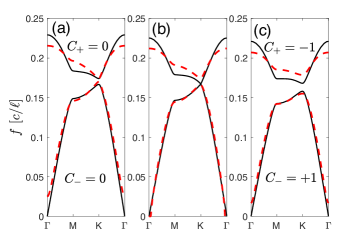
Figure 5: Topological transition of frequency Bloch bands as inversion symmetry is broken by decreasing the radius $R_{a}$ while keeping $R_{b}=0.3$. Numerical (solid curves) and tight-binding (dashed curves) approximations are shown for (a) $R_{a}=0.25\ell,(b)R_{a}=0.27\ell,\text{~{}and~{}}(c)R_{a}=0.3\ell$.

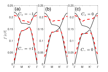
Figure 6: Spectral bands and topological transition when inversion symmetry is broken by increasing the radius $R_{a}$ while fixing $R_{b}=0.3\ell$. Numerical (solid curves) and tight-binding (dashed curves) approximations are shown for (a) $R_{a}=0.3\ell,$ (b) $R_{a}=0.35\ell,$ and (c) $R_{a}=0.4\ell.$

Specifically, for fixed radius $R_{b}=0.3\ell$, the (numerical) transition points between a trivial and nontrivial Chern insulator occurs at approximately $R_{a}=0.27\ell$ (at $k=K$; see Fig. 5(b)) and $R_{a}=0.35\ell$ (at $k=K^{\prime}$; see 6(b)). The discrete model (4)-(5) is also found to exhibit these topological transitions when the inversion symmetry is broken, i.e. $M\not=0$ in (6). The different regions of topology were analytically studied in Sec. IV.1; this information is summarized in Fig. 4.

We note that for values of $\tau$ smaller than 1, like Fig. 5, typically the difference $|R_{a}-R_{b}|$ for $R_{a}<R_{b}$ needs to be smaller to see a topological transition (numerical bands touch for $R_{a}=0.27\ell,R_{b}=0.3\ell$, so $|R_{a}-R_{b}|=0.03\ell$). In contrast, when $R_{a}>R_{b}$ and $\tau$ is larger than 1, like Fig. 6, a larger difference $|R_{a}-R_{b}|$ is needed for a topological transition (numerical bands touch for $R_{a}=0.35\ell,R_{b}=0.3\ell$, so $|R_{a}-R_{b}|=0.05\ell$). In examining the locations of the parameters (see Table 1 in Appendix B) relative to the topological regions shown in Fig. 4, it appears this source of the asymmetry is the noticeable change in the value $\phi$ as $R_{a}$ increases. This differs from the behavior when $R_{a}$ decreases, where $\phi$ does not change substantially. This asymmetry in the transition points also occurs if instead $R_{a}$ is fixed and $R_{b}$ is adjusted. The main difference is that the spectral touching points switch from what was observed above: $K\leftrightarrow K^{\prime}$.

V Topologically Protected Edge Modes

The edge problem is now considered. An edge is placed along the zig-zag edge parallel to the ${\bf v}_{1}$ lattice vector. Outside a semi-infinite strip, the electric field is assumed to decay exponentially fast. We find edge states that decay exponentially in the ${\bf v}_{2}$ direction. Two topologically distinct edge band diagrams are shown in Fig. 7. Edges modes along the direction ${\bf v}_{1}$ are found by taking

$$a_{mn}(t)=a_{n}({\bf k})e^{i\left[m{\bf k}\cdot{\bf v}_{1}+\omega t\right]},~{}b_{mn}(t)=b_{n}({\bf k})e^{i\left[m{\bf k}\cdot{\bf v}_{1}+\omega t\right]},$$

which reduces the governing system (4)-(5) to

$$\omega^{2}a_{n}=Pa_{n}+t_{1}\left[(1+e^{-i{\bf k}\cdot{\bf v}_{1}})b_{n}+b_{n-1}\right]$$ (16)

$$+ t_{2}e^{i\phi}\left[a_{n+1}+e^{-i{\bf k}\cdot{\bf v}_{1}}a_{n}+e^{i{\bf k}\cdot{\bf v}_{1}}a_{n-1}\right]$$

$$+ t_{2}e^{-i\phi}\left[a_{n-1}+e^{i{\bf k}\cdot{\bf v}_{1}}a_{n}+e^{-i{\bf k}\cdot{\bf v}_{1}}a_{n+1}\right]=0,$$

$$\omega^{2}b_{n}=\widetilde{P}b_{n}+t_{1}\left[(1+e^{i{\bf k}\cdot{\bf v}_{1}})a_{n}+a_{n+1}\right]$$ (17)

$$+ \tilde{t}_{2}e^{-i\phi}\left[b_{n+1}+e^{-i{\bf k}\cdot{\bf v}_{1}}b_{n}+e^{i{\bf k}\cdot{\bf v}_{1}}b_{n-1}\right]$$

$$+ \tilde{t}_{2}e^{i\phi}\left[b_{n-1}+e^{i{\bf k}\cdot{\bf v}_{1}}b_{n}+e^{-i{\bf k}\cdot{\bf v}_{1}}b_{n+1}\right]=0.$$

Note that ${\bf k}\cdot{\bf v}_{1}=(r{\bf k}_{1}+s{\bf k}_{2})\cdot{\bf v}_{1}=2\pi r$ for $r,s\in\mathbb{R}$ due to the relationship ${\bf k}_{i}\cdot{\bf v}_{j}=2\pi\delta_{ij}$. As a result, the coefficients cover one period over $0\leq r\leq 1$. This system is solved numerically by implementing zero Dirichlet boundary conditions

$$a_{n},b_{n}=0,~{}~{}~{}~{}n<0,n>N$$

where $N$ is taken to be large. We took $N=64$ to generate Fig. 7. The band gap eigenfunctions are found to be exponentially localized and decay rapidly away from the boundary wall, in the ${\bf v}_{2}$ direction.

The band configuration in Fig. 7(a^′) corresponds to bulk eigenmodes with zero Chern number due strong inversion symmetry breaking. As a result, there are no edge modes spanning the entire frequency gap. On the other hand, the system with corresponding nonzero Chern numbers in Fig. 7(c^′) exhibits a nontrivial band structure inside the gap. These topologically protected chiral states propagate unidirectionally.

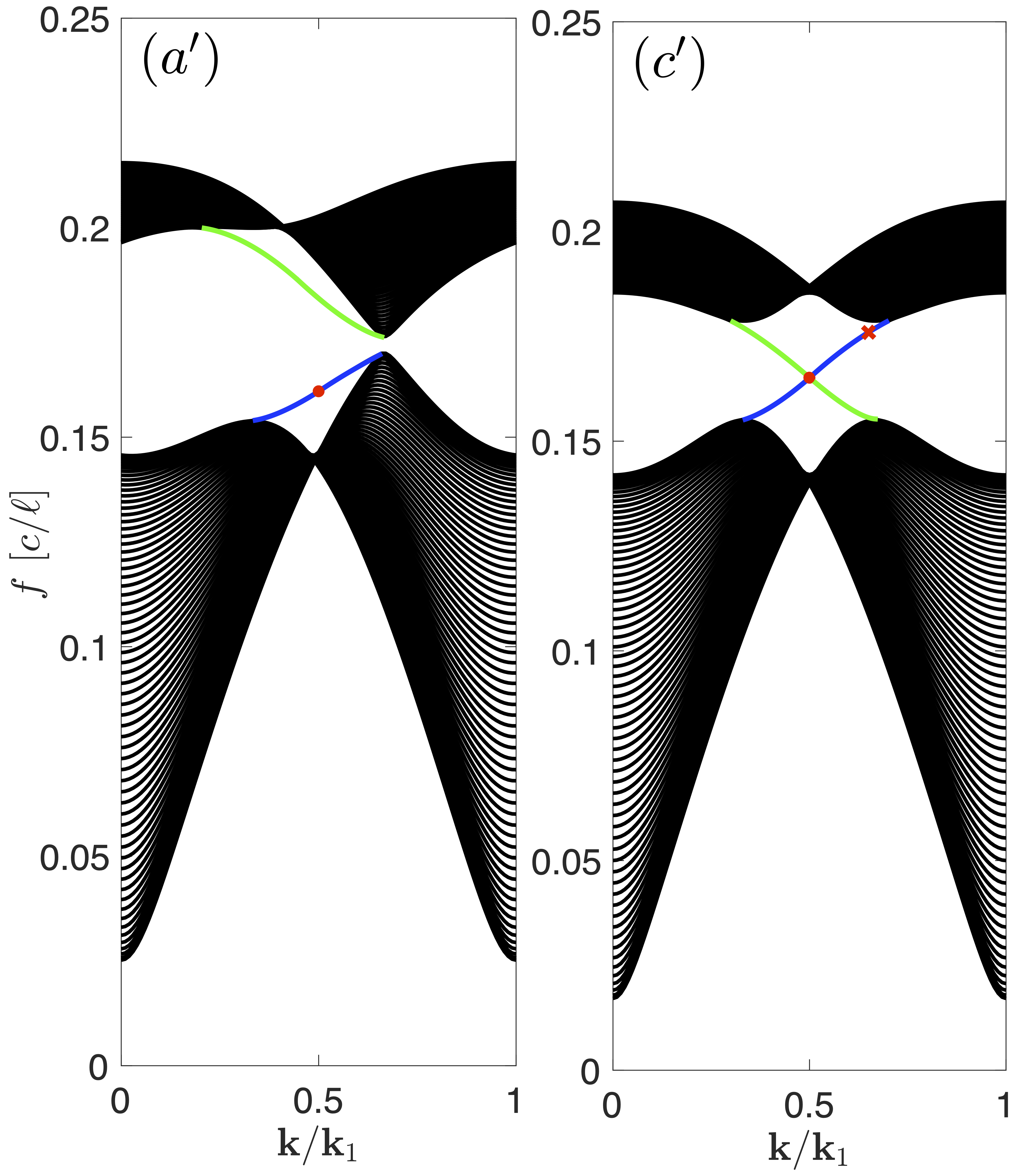
Figure 7: Spectral edge bands parallel to the ${\bf v}_{1}$ zig-zag edge. The model parameters for the (a^′) topologically trivial and (c^′) topologically nontrivial band diagrams are the same as those in Figs. 5(a) and 5(c), respectively. Green (blue) curves correspond to edge modes localized along the top (bottom) boundary, decaying in the $+{\bf v}_{2}$ ($-{\bf v}_{2}$) direction.

Finally, we consider time evolutions of these topologically distinct states. To do so, envelope approximations are evolved by taking the quasi-monochromatic initial data

$$a_{mn}(0)={\rm sech}(\nu m)e^{im\overline{\bf k}\cdot{\bf v}_{1}}a_{n}(\overline{\bf k})$$

$$b_{mn}(0)={\rm sech}(\nu m)e^{im\overline{\bf k}\cdot{\bf v}_{1}}b_{n}(\overline{\bf k}),$$

where $a_{n},b_{n}$ are numerically computed edge states indicated by the red dots at $\overline{\bf k}=0.5{\bf k}_{1}$ in Fig. 7 and $\nu$ is a relatively small parameter; here we took $\nu=0.1$. Edge eigenmodes corresponding to localized along the bottom edge of MO honeycomb lattice are taken. The edge envelopes are then propagated into a defect barrier missing two lattice cells in the $-{\bf v}_{2}$ direction, in which the electric field is negligibly small.

Using the initial condition above, the evolutions obtained by solving (4)-(5) are highlighted in Fig. 8. Edge states with corresponding nontrivial Chern invariants (see Figs. 7(c^′) and 8(c^′′)) propagate chiraly around the defect barrier. There is virtually no loss in amplitude. On the other hand, edge modes associated with zero Chern number (see Figs. 7(a^′) and 8(a^′′)) experience significant losses and scattering upon collision with the barrier. A portion of the original envelope propagates around the barrier, but there is a nearly 67% amplitude loss due to scattering into the bulk.

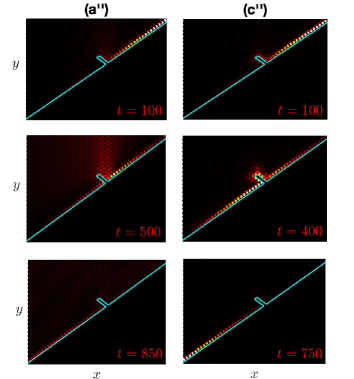
Figure 8: Envelope evolutions along and through a defect barrier. Shown are both magnitudes $|a_{mn}(t)|$ and $|b_{mn}(t)|$ at times in units of $\ell/c$. Shown are (a^′′) trivial and (c^′′) nontrivial Chern insulators with band diagrams given in Figs. 7(a^′) and 7(c^′), respectively. Note: brightness is relative to the $t=100$ magnitude. The boundary is illustrated in teal color.

As a final note, we observe small decay in the maximal amplitude of the these topologically protected modes, a roughly $10\%$ decline over $1500$ time units. This is expected due to dispersion. It is well-known that self-focusing nonlinearity can balance these dispersive effects and form solitons Ablowitz_book . This motivates this next section which investigates a nonlinear Haldane model and edge solitons.

VI A Nonlinear Haldane Model

In this section, we consider the effects of nonlinearity in our Haldane model. Similar versions of this model were mentioned in the Introduction section. The physical motivation here is that of a (relatively) high power electric field with non-negligible third-order polarization effects. The result is an onsite Kerr-type term that is proportional to the field intensity.

We consider the following nonlinear Haldane model

$$\frac{d^{2}a_{mn}}{dt^{2}} +Pa_{mn}+t_{1}(\delta_{-}b_{mn})+\sigma|a_{mn}|^{2}a_{mn}$$ (18)

$$+t_{2}e^{i\phi}(\Delta_{1}a_{mn})+t_{2}e^{-i\phi}(\Delta_{2}a_{mn})=0$$

$$\frac{d^{2}b_{mn}}{dt^{2}} +\widetilde{P}b_{mn}+t_{1}(\delta_{+}a_{mn})+\sigma|b_{mn}|^{2}b_{mn}$$ (19)

$$+\tilde{t}_{2}e^{-i{\phi}}(\Delta_{1}b_{mn})+\tilde{t}_{2}e^{i{\phi}}(\Delta_{2}b_{mn})=0$$

where the linear interaction coefficients, $\delta_{\pm},\Delta_{j},j=1,2$, are defined below (4)-(5). Motivated by previous studies, we take an on-site focusing, Kerr-type nonlinearity, i.e. $\sigma>0$. For the simulations below, we take $\sigma=0.1$.

The initial conditions used to generate solitons below are of the form

$$a_{mn}(0)=A~{}{\rm sech}(\nu m)e^{im\overline{\bf k}\cdot{\bf v}_{1}}a_{n}(\overline{\bf k})$$

$$b_{mn}(0)=A~{}{\rm sech}(\nu m)e^{im\overline{\bf k}\cdot{\bf v}_{1}}b_{n}(\overline{\bf k}),$$

with $\overline{\bf k}=0.65{\bf k}_{1}$. We choose a linear edge mode whose corresponding dispersion (second-derivative) is nonzero, i.e. $\omega^{\prime\prime}\left(\overline{\bf k}\right)\approx-0.287<0$ (see red ‘x’ marker in Fig. 7). Note that these derivatives are defined in the directional derivative sense

$$\omega^{\prime}({\bf k})=\nabla\omega|_{\bf k_{1}}=\lim_{h\rightarrow 0}\frac{\omega({\bf k}+h{\bf k}_{1})-\omega({\bf k})}{h}.$$

For reference, the group velocity is $\omega^{\prime}\left(\overline{\bf k}\right)\approx-0.0584$ in the ${\bf v}_{1}$ direction. Unfortunately, the third order dispersion is relatively large, $\omega^{\prime\prime\prime}\left(\overline{\bf k}\right)\approx-1.401$ which will impact the formation of solitons. For this relatively weak dispersion, we seek a comparable weak nonlinearity to balance it, i.e. $A=0.3$. A corresponding slowly-varying profile ($\nu=0.15$) is chosen to ensure as pure of a single edge mode as possible is excited.

Using the parameters described above, a typical evolution thorough a one lattice cell defect in the $-{\bf v}_{2}$ direction is highlighted in Fig. 9. The resulting nonlinear mode propagates over relatively long time scales ($0\leq t\leq 1200$) with a nearly constant solitary form. We observe a small $3.7\%$ relative change in maximum magnitude between the initial and final states. Hence, we refer to this as an edge soliton. We note that, eventually, on longer time scales higher-order dispersion terms will become non-negligible and the mode will degrade.

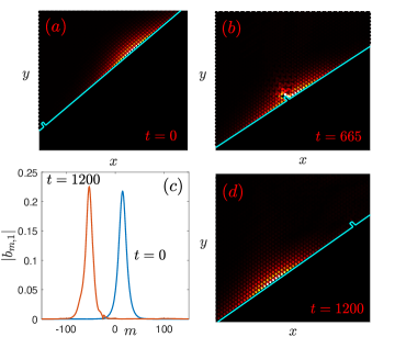
Figure 9: Nonlinear edge soliton evolutions through a defect. Shown in panels (a,b,d) are both magnitudes $|a_{mn}(t)|$ and $|b_{mn}(t)|$ at times in units of $\ell/c$. Note: brightness is relative to the $t=0$ magnitude. The boundary is illustrated in teal color; the defect location is fixed. In panel (c) the edge profile at the initial and final times is shown.

Now, some further remarks about these topologically protected edge solitons. Choosing the appropriate sign of dispersion is imperative for achieving a self-focusing effect and solitons. When $\omega^{\prime\prime}({\bf k})>0$, we observe a gradual self-defocusing dissipation of the envelope. The ideal scenario for soliton formation in this MO lattice is a when $\omega^{\prime\prime}({\bf k})<0$ and $\omega^{\prime\prime\prime}({\bf k})\approx 0$. Choosing a mode centered at the zero-dispersion (inflection) point, i.e. $\omega^{\prime\prime}({\bf k})=0$, results in substantial dispersive break-up of initially localized solitary waves.

In the nonlinear case, when we send a slowly-modulated mode corresponding to topologically trivial (null Chern number) into a defect, we observe significant radiation into the bulk, similar to that observed in Fig. 8(c”) for the linear evolution. In this weakly nonlinear regime, it is important to modulate a topologically nontrivial linear mode to obtain robust, unidirectional propagation. For a fully robust edge soliton, this nontrivial topology must be paired with a balanced soliton envelope.

VII Conclusion

A perturbed Wannier approach for obtaining tight-binding approximations containing nearest and next-nearest neighbors of a magneto-optical honeycomb lattice system is studied. Remarkably, this method leads to the celebrated system studied by Haldane in 1988 4. This model agrees with experiments Poo2011 and indicates topological transitions can occur when inversion symmetry and time-reversal symmetry are broken. This data-driven Wannier approach has been previously employed in rectangular lattice geometries Ablowitz2020 and can be applicable for discovering and extrapolating discrete reductions in other Chern insulator systems in cases where a direct Wannier approach is ineffective.

Acknowledgements This project was partially supported by AFOSR under grants No. FA9550-19-1-0084 and No. FA9550-23-1-0105.

Appendix A Numerical Computation of Spectral Bands and Wannier Functions

The numerical computation of the Bloch modes and maximally localized Wannier functions (MLWFs) is reviewed below. A more comprehensive discussion can be found in Ablowitz2020 . To simplify the necessary calculations, first, a linear transformation is introduced to map the parallelogram unit cell to a square. The change of variables

$$u=\frac{1}{3}x-\frac{1}{\sqrt{3}}y,~{}~{}~{}~{}~{}~{}v=\frac{1}{3}x+\frac{1}{\sqrt{3}}y$$

transforms the parallelogram formed by the lattice vectors ${\bf v}_{1},{\bf v}_{2}$ into a square with side length 1. As a result, the master equation (II) transforms to

$$-\frac{4}{9}\left(\frac{\partial^{2}E}{\partial u^{2}}-\frac{\partial^{2}E}{\partial u\partial v}+\frac{\partial^{2}E}{\partial v^{2}}\right) +g(u,v)\frac{\partial E}{\partial u}+h(u,v)\frac{\partial E}{\partial v}$$

$$=\omega^{2}\varepsilon(u,v)\tilde{\mu}(u,v)E$$ (20)

where

$$g(u,v)=\frac{4}{9\tilde{\mu}}\frac{\partial\tilde{\mu}}{\partial u}-\frac{2}{9\tilde{\mu}}\frac{\partial\tilde{\mu}}{\partial v}+\frac{2i\tilde{\mu}}{3\sqrt{3}}\frac{\partial\eta}{\partial v}$$

$$h(u,v)=-\frac{4}{9\tilde{\mu}}\frac{\partial\tilde{\mu}}{\partial u}+\frac{2}{9\tilde{\mu}}\frac{\partial\tilde{\mu}}{\partial v}-\frac{2i\tilde{\mu}}{3\sqrt{3}}\frac{\partial\eta}{\partial v}.$$

From here, a formulation similar to that used in Ablowitz2020 can be applied. All transformed coefficients now have the periodicity: $f(u+m,v+n)=f(u,v)$ for $m,n\in\mathbb{Z}$. That is, the functions are periodic with respect to the transformed lattice vectors ${\bf e}_{1}=(1,0)^{T}$ and ${\bf e}_{2}=(0,1)^{T}$. Hence, transformed master equation (A) is solved by looking for Bloch wave solutions with the form $E({\bf w},{\bm{\kappa}})=e^{i{\bm{\kappa}}\cdot{\bf w}}u({\bf w};{\bm{\kappa}})$, where $u({\bf w}+m{\bf e}_{1}+n{\bf e}_{2};{\bm{\kappa}})=u({\bf w};{\bm{\kappa}})$ for ${\bf w}=(u,v)^{T},{\bm{\kappa}}=(k_{u},k_{v})^{T}$. Note: this ${\bm{\kappa}}$ is unrelated to $\kappa$ of the permeability tensor.

The numerical spectral bands shown throughout this paper are computed by solving (A) for the eigenfunction/eigenvalue pair $(u,\omega)$ as functions of the transformed quasimomentum. Subsequently, the quasimomentum is transformed back to the original $k_{x},k_{y}$ variables via

$$k_{x}=\frac{k_{u}+k_{v}}{3},~{}~{}~{}~{}~{}~{}~{}k_{y}=\frac{k_{v}-k_{u}}{\sqrt{3}}.$$

The continuous Chern numbers are defined by

$$C_{p}=\frac{1}{2\pi i}\iint_{\rm BZ}(\nabla_{\bf k}\times{\bf A}_{p})\cdot\widehat{{\bf z}}~{}d{\bf k}~{},$$

where ${\bf A}_{p}({\bf k})=\langle u_{p}({\bf r},{\bf k})|\partial_{k_{x}}u_{p}({\bf r},{\bf k})\rangle_{{\rm UC},\epsilon\tilde{\mu}}~{}\widehat{\bf x}+\langle u_{p}({\bf r},{\bf k})|\partial_{k_{y}}u_{p}({\bf r},{\bf k})\rangle_{{\rm UC},\epsilon\tilde{\mu}}~{}\widehat{\bf y}$ are numerically computed using the algorithm fukui with respect to the weighted inner product

$$\langle f,g\rangle_{{\rm UC},\epsilon\tilde{\mu}}=\iint_{\rm UC}f({\bf r})^{*}g({\bf r})\varepsilon({\bf r})\tilde{\mu}({\bf r})d{\bf r},$$

where ${\rm UC}$ denotes the unit cell.

The transformed Bloch wave is periodic with respect to the transformed reciprocal lattice vectors, ${\bm{\kappa}}_{1}=2\pi(1,0)^{T},{\bm{\kappa}}_{2}=2\pi(0,1)^{T}$. Notice: ${\bf e}_{i}\cdot{\bm{\kappa}}_{j}=2\pi\delta_{ij}$. As such, it can be expressed as the Fourier series

$$E({\bf w};{\bm{\kappa}})=\sum_{p}\sum_{m,n}W_{mn}^{p}({\bf w})e^{i{\bm{\kappa}}\cdot(m{\bf e}_{1}+n{\bf e}_{2})},$$

where $W_{mn}^{p}({\bf w})$ is a transformed Wannier function corresponding to the $p^{\rm th}$ band, and centered at the $(m,n)$ unit cell. For the problem studied in this paper, we only consider the lowest two bands $p=1,2$ and truncate the remaining terms.

Next, the MLWF algorithm Marzari1997 is applied to find localized Wannier functions for the $g=h=0$ (corresponding to $\mathcal{M}={\bf 0}$) problem in equation (A). This is done by finding a unitary transformation that minimizes the functional describing the variance of the Wannier function, given by equation (21) below. Let $E_{1}({\bf w},{\bm{\kappa}})=e^{i{\bm{\kappa}}\cdot{\bf w}}u_{1}({\bf w};{\bm{\kappa}})$ and $E_{2}({\bf w},{\bm{\kappa}})=e^{i{\bm{\kappa}}\cdot{\bf w}}u_{2}({\bf w};{\bm{\kappa}})$ correspond to first and second spectral bands, respectively. A spectral unitary transformation of the Bloch functions is taken at fixed values of ${\bf w}$

$$\begin{pmatrix}\widetilde{u}^{c}({\bf w};{\bm{\kappa}})\\ \widetilde{u}^{d}({\bf w};{\bm{\kappa}})\end{pmatrix}=\mathbb{U}({\bm{\kappa}})\begin{pmatrix}{u}_{1}({\bf w};{\bm{\kappa}})\\ {u}_{2}({\bf w};{\bm{\kappa}})\end{pmatrix}$$

where $\mathbb{U}({\bm{\kappa}})$ is a $2\times 2$ matrix. Only after computing these Wannier functions do we realize where they are physically located. Upon inspection, we replace the labels $c,d$ with the labels $a,b$, where $a$ modes are centered at the $a$-sites and $b$ modes centered at the $b$-sites (see Fig. 3).

Upon obtaining these functions, the Bloch modes $\widetilde{E}^{a}({\bf w};{\bm{\kappa}})=e^{i{\bm{\kappa}}\cdot{\bf w}}\widetilde{u}^{a}({\bf w};{\bm{\kappa}})$ and $\widetilde{E}^{b}({\bf w};{\bm{\kappa}})=e^{i{\bm{\kappa}}\cdot{\bf w}}\widetilde{u}^{b}({\bf w};{\bm{\kappa}})$ are computed and then used to construct the Wannier functions

$$\widetilde{W}^{a}_{mn}({\bf w})=\frac{1}{4\pi^{2}}\iint_{\rm BZ}e^{-i{\bm{\kappa}}\cdot(m{\bf e}_{1}+n{\bf e}_{2})}\widetilde{E}^{a}({\bf w};{\bm{\kappa}})d{\bm{\kappa}}$$

$$\widetilde{W}^{b}_{mn}({\bf w})=\frac{1}{4\pi^{2}}\iint_{\rm BZ}e^{-i{\bm{\kappa}}\cdot(m{\bf e}_{1}+n{\bf e}_{2})}\widetilde{E}^{b}({\bf w};{\bm{\kappa}})d{\bm{\kappa}}$$

shown in Fig. 3.

Appendix B Tight-binding Parameters

The parameters used to produce the tight-binding approximations are given in Table 1. All cases correspond to the magnetization by an external field, or $\mathcal{M}({\bf r})\not={\bf 0}$, except (i) which is the unmagnetized case. Also included are the corresponding rod radii. The Chern number corresponding to the upper spectral surface of the tight-binding model is included. The value $C_{+}=-1$ corresponds to phase points located inside the topological region of Fig. 4, while $C_{+}=0$ lies above or below this region. The values in the table were computed analytically as well as numerically using the algorithm in fukui on the discrete eigenvectors. In all cases considered, the values agreed. The topological numbers for the discrete (tight-binding) model also match those for the continuum model, except possibly near the sensitive topological transition points.

	$R_{a}$	$R_{b}$	$P$	$\widetilde{P}$	$t_{1}$	$t_{2}$	$\tilde{t}_{2}$	$\phi$	$C_{+}$
(i)	$0.3\ell$	$0.3\ell$	0.882	0.882	-0.262	0.012	0.012	$\pi$	0
(ii)	$0.3\ell$	$0.3\ell$	1.020	1.020	-0.280	0.041	0.041	2.327	-1
(iii)	$0.27\ell$	$0.3\ell$	1.152	0.991	-0.297	0.049	0.037	2.391
(iv)	$0.25\ell$	$0.3\ell$	1.263	0.973	-0.300	0.055	0.030	2.405	0
(v)	$0.35\ell$	$0.3\ell$	0.876	1.077	-0.265	0.031	0.048	2.178
(vi)	$0.4\ell$	$0.3\ell$	0.790	1.132	-0.263	0.024	0.053	1.941	0

Table 1: Tight-binding parameters in (4)-(5) for (i) non-magnetized bands and magnetized (ii-vi) systems. The rod radii used to generate these parameters are given by $R_{a}$ and $R_{b}$ for a-sites and b-sites, respectively. The value of $C_{+}$ indicates the Chern number corresponding to the second (upper) spectral band.

Appendix C Breaking of Inversion Symmetry

As discussed in Sec. IV.2, breaking inversion symmetry can induce a topological transition from a nontrivial to trivial Chern insulator. This symmetry breaking can be implemented by choosing different radii at a-sites and b-sites, that is $R_{a}\not=R_{b}$ in Fig. 1. The spectral bands induced by this change are shown in Figs. 5 and 6. In particular, decreasing $R_{a}$ relative to $R_{b}$ induces a topological transition and a touching point at the $K$ Dirac point. If, on the other hand, one considers $R_{a}$ larger relative to $R_{b}$, a similar topological transition occurs, but instead the gap closes at the opposite Dirac point, $K^{\prime}=-K$. A depiction of this is shown in Fig. 6.

The computed parameters are summarized in Table 1. Examining the inversion parameter $M=(P-\widetilde{P})/2$, it is observed to be positive when $R_{a}<R_{b}$, and negative when $R_{a}>R_{b}$. For applications which seek to use these chiral edge modes, inversion symmetry should be nearly satisfied, that is, $R_{a}\approx R_{b}$. More precisely, the system supports topologically protected modes when the parameters $\widetilde{M}$ and $\phi$ are chosen to reside in the inner (topological) region of Fig. 4.

Some of the Wannier functions corresponding to broken inversion symmetry are shown in Fig. 10. In each case the rod profiles and their corresponding Wannier modes are shown. These Wannier modes are constructed in a manner similar to that described in Sec. III and Ablowitz2020 , i.e. $\mathcal{M}={\bf 0},\tilde{\mu}\not=\mu_{0}$. Also given is the variance

$$\Omega=\langle|{\bf r}|^{2}\rangle-|\langle{\bf r}\rangle|^{2},$$ (21)

$$\langle x^{n}\rangle\equiv\iint_{\mathbb{R}^{2}}x^{n}|W({\bf r})|^{2}\varepsilon({\bf r})\tilde{\mu}({\bf r})d{\bf r}$$

where $W({\bf r})$ is the corresponding Wannier mode. The lattice sites whose rods have larger relative radius, correlate to a smaller variances; and vice versa for smaller relative rods. This is the source of $\tilde{t}_{2}\not=t_{2}$ and $P\not=\widetilde{P}$. These different widths indicate different decay rates and imply different tight-binding coefficients among sites of the same type.

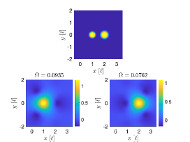
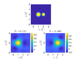
Figure 10: The top row panels highlight the rod radii for the different cases. Bottom rows show the maximally localized Wannier functions (MLWFs) corresponding to those physical parameters. (left) Radii: $R_{a}=0.25\ell,R_{b}=0.3\ell$ and (right) Radii: $R_{a}=0.4\ell,R_{b}=0.3\ell$. Also included for each Wannier function is the corresponding width, defined in (21).

References

- (1) G. Jotzu, M. Messer, Rémi Desbuquois, M. Lebrat, T. Uehlinger, D. Greif, and T. Esslinger, Nature 515 237 (2014).
- (2) K. Von Klitzing, G. Dorda, and M. Pepper, Phys. Rev. Lett. 45 494 (1980).
- (3) B. A. Bernevig and S.-C. Zhang, Phys. Rev. Lett. 96 106802 (2006).
- (4) C.-Z. Chang, et al., Science 340 167 (2013).
- (5) P. Delplace, J. B. Marston, and A. Venaille, Science 358 1075 (2017).
- (6) M. C. Rechtsman, et al., Nature 496 196 (2013).
- (7) T. Ozawa, H. M. Price, A. Amo, N. Goldman, M. Hafezi, L. Lu, M. C. Rechtsman, D. Schuster, J. Simon, O. Zilberberg, and I. Carusotto, Rev. Mod. Phys. 91 015006 (2019).
- (8) L. Lu, J. D. Joannopoulos, and M. Soljac̆ić, Nat. Photon. 8 821 (2014).
- (9) M. J. Ablowitz and J. T. Cole, Physica D 440 133440 (2022).
- (10) C. L. Fefferman, J. P. Lee‐Thorp, M. I. Weinstein, Comm. Pure Appl. Math. 71 1178 (2018).
- (11) F. D. M. Haldane, Phys. Rev. Lett. 61 2015 (1988).
- (12) Z. Wang, Y. D. Chong, J. D. Joannopoulos, and M. Soljac̆ić, Phys. Rev. Lett. 100 013905 (2008).
- (13) Z. Wang, Y. D. Chong, J. D. Joannopoulos, and M. Soljac̆ić, Nature 461 772 (2009).
- (14) X.-C. Sun, C. He, X.-P. Liu, Y. Zou, M.-H. Lu, X. Hu, and Y.-F. Chen, Crystals 9 137 (2019).
- (15) Y. Yang, Y. Poo, R.-X. Wu, Y. Gu, and P. Chen, Appl. Phys. Lett. 102 231113 (2013).
- (16) X. Ao, Z. Lin, and C. T. Chan, Phys. Rev. B 80 033105 (2009).
- (17) Y. Poo, R.-X. Wu, Z. Lin, Y. Yang, and C. T. Chan, Phys. Rev. Lett. 106 093903 (2011).
- (18) R. Zhao, G.-D. Xie, M. L. N. Chen, Z. Lan, Z. Huang, and W. E. I. Sha, Opt. Express 28 4638 (2020).
- (19) F. D. M. Haldane and S. Raghu, Phys. Rev. Lett. 100 013904 (2008).
- (20) S. Raghu and F. D. M. Haldane, Phys. Rev. A 78 033834 (2008).
- (21) J. P. Lee-Thorp, M. I. Weinstein, Y. Zhu, Arch. Ration. Mech. Anal. 232 1 (2019).
- (22) M. J. Ablowitz, J. T. Cole, and S. D. Nixon, SIAM J. Appl. Math., In press, (2023)
- (23) M. J. Ablowitz and J. T. Cole, Phys. Rev. A 101 023811 (2020).
- (24) M. J. Ablowitz, C. W. Curtis, and Y.-P. Ma, Phys. Rev. A 90 023813 (2014).
- (25) M. J. Ablowitz and J. T. Cole, Phys. Rev. A 96 043868 (2017).
- (26) S. Mukherjee and M. C. Rechtsman, Phys. Rev. X 11 041057 (2021).
- (27) M. J. Ablowitz, J. T. Cole, P. Hu, and P. Rosenthal, Phys. Rev. E 103 042214 (2021).
- (28) G. Harari, et al., Science 359 eaar4003 (2018).
- (29) X. Zhou, Y. Wang, D. Leykam, and Y. D. Chong, New J. Phys. 19 095002 (2017).
- (30) C. Brouder, G. Panati, M. Calandra, C. Mourougane, and N. Marzari, Phys. Rev. Lett. 98 046402 (2007).
- (31) N. Marzari and D. Vanderbilt, Phys. Rev. B 56 12847 (1997).
- (32) D. M. Pozar, Microwave Engineering 4th ed. (John Wiley & Sons, 2012).
- (33) T. Fukui, Y. Hatsugai, and H. Suzuki, Phys. Soc. of Japan, 74 1674 (2005).
- (34) M. J. Ablowitz, Nonlinear Dispersive Waves (Cambridge Press, 2011).