Phases and Exotic Phase Transitions
of a Two-Dimensional Su-Schrieffer-Heeger Model

Abstract

We study a Su-Schrieffer-Heeger electron-phonon model on a square lattice by means of auxiliary-field quantum Monte Carlo simulations. The addition of a symmetry-allowed interaction permits analytical integration over the phonons at the expense of discrete Hubbard-Stratonovich fields with imaginary-time correlations. Using single-spin-flip updates, we investigate the phase diagram at the O(4)-symmetric point as a function of hopping $t$ and phonon frequency $\omega_{0}$. For $t=0$, where electron hopping is boson-assisted, the model maps onto an unconstrained $\mathbb{Z}_{2}$ gauge theory. A key quantity is the emergent effective flux per plaquette, which equals $\pi$ in the assisted-hopping regime and vanishes for large $t$. Phases in the former regime can be understood in terms of instabilities of emergent Dirac fermions. Our results support a direct and continuous transition between a $(\pi,0)$ valence bond solid (VBS) and an antiferromagnetic (AFM) phase with increasing $\omega_{0}$. For large $t$ and small $\omega_{0}$, we find finite-temperature signatures of a previously reported $(\pi,\pi)$ VBS ground state related to a nesting instability. With increasing $\omega_{0}$, AFM order again emerges.

I Introduction

One of the most fundamental interaction channels in the solid state is the coupling between lattice vibrations (phonons) and conduction electrons. In a Fermi liquid with a coherence temperature orders of magnitude greater than the Debye frequency, electron-phonon coupling leads to a retarded and net attractive interaction. The Cooper instability of Fermi surfaces promotes superconductivity [1, 2]. However, electron-phonon coupling does not always lead to superconductivity. Notably, in one-dimension (1D), where $2k_{\text{F}}$ nesting is generic, it triggers a Peierls charge-density-wave (CDW) instability. In 2D systems, nested Fermi surfaces lead to, e.g., $(\pi,\pi)$ valence bond solid (VBS) or antiferromagnetic (AFM) order [3, 4].

Here, we investigate if a symmetry-allowed generalization of the Su-Schrieffer-Heeger (SSH) model [5] on a square lattice can host exotic phases and quantum phase transitions. This question has previously been answered affirmatively for a spinless 1D SSH model, which exhibits instances of 1D deconfined quantum criticality [6, 7, 8, 9].

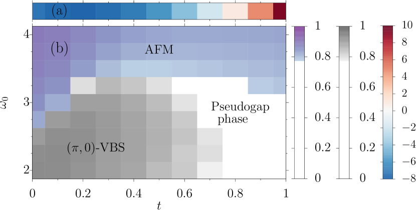
Figure 1: Phase diagram of Hamiltonian (3) as a function of electronic hopping $t$ and phonon frequency $\omega_{0}$, based on QMC simulations. It features antiferromagnetic (AFM), valence-bond solid (VBS), and pseudogap phases. At small $t$, we observe the spontaneous generation of a $\pi$-flux in each plaquette. (a) Average flux $\langle\hat{\Phi}_{\bm{i}}\rangle$ as a function of $t$ at $\omega_{0}=2.0$, (b) correlation ratio of the spin susceptibility $R_{\chi,S}$ at $(\pi,\pi)$ (lilac scale) and the VBS susceptibility $R_{\chi,D(\pi,0)}$ at $(\pi,0)$ (gray scale). Results in panels (a) and (b) are for $L=\beta=8$. Here, $\tilde{g}=\sqrt{2/k}g=2$ and $\lambda=0.5$.

From the original perspective of electron-phonon coupling, the phonon-mediated modulation of the direct hopping $t$ in the SSH model has to be small [5]. However, we can take a more general view by also considering the regime of small (vanishing) $t$, where electronic hopping is partially (exclusively) phonon-assisted. Related fermion-boson models have been put forward to describe the motion of holes in an antiferromagnetic background [10] . Similar to Ref. [12], our model includes an additional electronic interaction term (the square of the hopping) to facilitate integration over the phonons without generating a sign problem in quantum Monte Carlo (QMC) simulations. We used an implementation of the finite-temperature auxiliary-field QMC algorithm [13, 14, 15, 16] from the Alogrithms for Lattice Fermions (ALF) package [17].

The main results are summarized by the very rich phase diagram in Fig. 1. At $t=0$, our model maps onto an unconstrained $\mathbb{Z}_{2}$ lattice gauge theory [18, 19, 20]. In this limit, a $\pi$-flux per plaquette and associated Dirac fermions emerge. Importantly, the $t=0$ physics is adiabatically connected to a $t>0$ region where the flux remains negative, in which we observe dynamically generated mass terms corresponding to $(\pi,0)$ VBS and AFM phases. The latter are separated by an apparently direct and continuous phase transition interpreted as a deconfined quantum critical point (DQCP) [6, 21]. At large $t$, the $\pi$-flux vanishes and previous studies [22, 3, 4, 23, 24] suggest the ground state at small $\omega_{0}$ to be a $(\pi,\pi)$ VBS state. At the temperatures considered here, we instead observe a pseudogap phase of fluctuating dimers.

The paper is organized as follows. In Sec. II, we define the model and discuss its symmetries and limiting cases, as well as previous work. In Sec. III, we describe our numerical method. In Sec. IV, we present our numerical results, followed by a discussion and conclusions in Sec. V. We provide four appendices with further details about the method and additional data, respectively.

II Model and Symmetries

II.1 Model

A generic SSH-type Hamiltonian [5, 25] with Einstein phonons takes the form

$$\hat{H}=\sum_{b}\left(-t+g\hat{X}_{b}\right)\hat{K}_{b}+\sum_{b}\left(\frac{1}{2m}\hat{P}_{b}^{2}+\frac{k}{2}\hat{X}_{b}^{2}\right)\,.$$ (1)

The first term describes fermion hopping and fermion-phonon coupling on bonds $b=\langle\bm{i},\bm{j}\rangle$ connecting nearest-neighbor sites $\bm{i}$ and $\bm{j}$, with the hopping operator

$$\hat{K}_{b}=\sum_{\sigma}\hat{c}_{\bm{i},\sigma}^{\dagger}\hat{c}_{\bm{j},\sigma}^{\phantom{\dagger}}+\mathrm{H.c.}=\sum_{\bm{i},\bm{j},\sigma}\hat{c}^{\dagger}_{\bm{i},\sigma}\left(K_{b}\right)_{\bm{i},\bm{j}}\hat{c}^{\phantom{\dagger}}_{\bm{j},\sigma}\,.$$ (2)

Here, $\left(K_{b}\right)_{\bm{i},\bm{j}}=1$ if $\bm{i}$ and $\bm{j}$ are nearest neighbors and $0$ otherwise. The operator $\hat{c}_{\bm{i},\sigma}^{\dagger}$ creates a fermion in a Wannier state centered at site $\bm{i}$ and with $z$-component of spin equal to $\sigma$. We will keep the notation general enough to allow for the case of $N$ fermion flavors. However, all numerical results will be for $N=2$, corresponding to electrons with spin $1/2$. The strength of the bare electron hopping is set by the hopping integral $t$, whereas $g$ determines the electron-phonon coupling, which modulates the electronic hopping. The second term in Eq. (1) describes bond phonons modeled as harmonic oscillators with position operators $\hat{X}_{b}$, momentum operators $\hat{P}_{b}$, and frequency $\omega_{0}^{2}=k/m$.

Here, we study the slightly different Hamiltonian

$$\hat{H}=\sum_{b}(-t+g\hat{X}_{b})\hat{K}_{b}-\lambda\sum_{b}\hat{K}_{b}^{2}+\sum_{b}\left(\frac{1}{2m}\hat{P}_{b}^{2}+\frac{k}{2}\hat{X}_{b}^{2}\right)$$ (3)

on a square lattice with $N_{s}=L\times L$ sites. Compared to Eq. (1), we include an additional electronic interaction $-\lambda\hat{K}_{b}^{2}$ to complete the square and facilitate integration over the phonons, similar to recent work on the Hubbard-Holstein model [12]. The additional term does not alter the symmetries of the model and will therefore also be dynamically generated.

II.2 Symmetries

For half-filling and a bipartite lattice, the Hamiltonian in Eq. (3) is invariant under the partial particle-hole transformation [here, $\bm{M}=(\pi,\pi)$]

$$\hat{P}^{-1}_{\sigma}\hat{c}_{\bm{i},\sigma^{\prime}}^{\dagger}\hat{P}_{\sigma}=\delta_{\sigma,\sigma^{\prime}}e^{i\bm{M}\cdot\bm{i}}\hat{c}_{\bm{i},\sigma^{\prime}}^{\phantom{\dagger}}+\left(1-\delta_{\sigma,\sigma^{\prime}}\right)\hat{c}_{\bm{i},\sigma}^{\dagger}\,.$$ (4)

The fermion parity on site $\bm{i}$ is given by

$$\hat{p}_{\bm{i}}=\prod_{\sigma=1}^{N}\left(1-2\hat{n}_{\bm{i},\sigma}\right)\,,$$ (5)

where $\hat{n}_{\bm{i},\sigma}=\hat{c}_{\bm{i},\sigma}^{\dagger}\hat{c}_{\bm{i},\sigma}^{\phantom{\dagger}}$ is the fermion number operator. The parity changes sign under transformation (4) and can be used to detect a spontaneous breaking of particle-hole symmetry. Because the parity is an Ising-like order parameter, $\hat{p}_{\bm{i}}^{2}=1$, it supports order at finite temperatures in the 2D case considered.

Our model further exhibits an $\mathrm{O}(2N)$ symmetry on bipartite lattices [3, 4]. To prove this, we use the Majorana representation for the fermions [18, 26],

$$\hat{c}_{\bm{i},\sigma}^{\dagger}=\frac{1}{2}\left(\hat{\gamma}_{\bm{i},\sigma,1}-i\hat{\gamma}_{\bm{i},\sigma,2}\right)\,.$$ (6)

With a canonical transformation $\hat{c}_{\bm{i}}^{\dagger}\rightarrow i\hat{c}_{\bm{i}}^{\dagger}$ on one sublattice, the hopping operator can be written as

$$\hat{K}_{b}=\sum_{\sigma=1}^{N}\left(\hat{c}^{\dagger}_{\bm{i},\sigma}\hat{c}^{\phantom{\dagger}}_{\bm{j},\sigma}+\text{h.c.}\right)=\frac{i}{2}\sum_{\sigma}\sum_{\alpha=1}^{2}\hat{\gamma}_{\bm{i},\sigma,\alpha}\hat{\gamma}_{\bm{j},\sigma,\alpha}\,,$$ (7)

thereby revealing the $\mathrm{O}(2N)$ symmetry. For the case $N=2$ considered here, the infinitesimal generators of the $\mathrm{O}(4)$ symmetry are the spin operators $\hat{\bm{S}}_{\bm{i}}=(\hat{S}^{x}_{\bm{i}},\hat{S}^{y}_{\bm{i}},\hat{S}^{z}_{\bm{i}})$ and the Anderson pseudospin operators $\hat{\bm{\eta}}_{\bm{i}}$ [27], given by

$$\hat{S}_{\bm{i}}^{\alpha}=\frac{1}{2}\sum_{\sigma,\sigma^{\prime}}\hat{c}_{\bm{i},\sigma}^{\dagger}(\tau^{\alpha})_{\sigma,\sigma^{\prime}}\hat{c}_{\bm{i},\sigma^{\prime}},\quad\hat{\bm{\eta}}_{\bm{i}}=\hat{P}_{\uparrow}^{-1}\hat{\bm{S}}_{\bm{i}}\hat{P}_{\uparrow}\,.$$ (8)

Here, $\tau^{\alpha}$ is a Pauli matrix with $\alpha=x,y,z$. The components of $\hat{\bm{S}}_{\bm{i}}$ and $\hat{\bm{\eta}}_{\bm{i}}$ fulfill the Lie algebra of the $\mathrm{SU}(2)$ group, $[\hat{S}_{\bm{i}}^{\alpha},\hat{S}_{\bm{j}}^{\beta}]=i\delta_{\bm{i},\bm{j}}\sum_{n}\varepsilon_{\alpha\beta\gamma}\hat{S}_{\bm{i}}^{\gamma}$ ($\varepsilon_{\alpha\beta\gamma}$ is the Levi-Civita symbol), and commute among each other, $[\hat{S}_{\bm{i}}^{\alpha},\hat{\eta}_{\bm{j}}^{\beta}]=0$. The Lie algebra of the global $\mathrm{O}(4)$ symmetry can be interpreted as $\mathrm{O}(4)=\mathrm{SU}(2)\times\mathrm{SU}(2)\times\mathbb{Z}_{2}$, where the additional $\mathbb{Z}_{2}$ symmetry corresponds to the partial particle-hole symmetry [18]. This implies that a potential AFM phase is degenerate with a CDW and an s-wave superconductor (SC). If the parity operator acquires a nonzero expectation value due to spontaneous breaking of the particle-hole symmetry, either the spin or the charge sector is explicitly chosen.

II.3 Limiting cases

II.3.1 Adiabatic limit $\omega_{0}=0$

In the adiabatic limit $\omega_{0}=0$, the phonons can be treated classically since quantum fluctuations are frozen out. The problem reduces to finding the phonon field configuration that minimizes the free energy of the mean-field Hamiltonian

$$\hat{H}=\sum_{b}(-t+gX_{b})\hat{K}_{b}+\frac{k}{2}\sum_{b}X_{b}^{2}-\lambda\sum_{b}\hat{K}_{b}^{2}\,.$$ (9)

The fields $X_{b}$ are defined as the eigenvalues of the position operator, $\hat{X}_{b}|x\rangle=X_{b}|x\rangle$. For $\lambda=0$, this model has been extensively studied, see Sec. II.4.

II.3.2 Anti-adiabatic limit $\omega_{0}\rightarrow\infty$

For $\omega_{0}>0$, we can integrate out the phonons. In the anti-adiabatic limit $\omega_{0}\rightarrow\infty$, the electron-phonon couplings reduces to an electronic interaction proportional to the square of the hopping operator [18, 4],

$$\hat{H}=-t\sum_{b}\hat{K}_{b}-\left(\lambda+\frac{g^{2}}{2k}\right)\sum_{b}\hat{K}_{b}^{2}\,.$$ (10)

For $N=2$ (i.e., spin $1/2$), it can be rewritten in terms of the generators of the $\mathrm{O}(4)$ symmetry,

$$-\frac{1}{4}\hat{K}_{b}^{2}=\hat{\bm{S}}_{\bm{i}}\cdot\hat{\bm{S}}_{\bm{j}}+\hat{\bm{\eta}}_{\bm{i}}\cdot\hat{\bm{\eta}}_{\bm{j}}\,.$$ (11)

For $\omega_{0}\rightarrow\infty$, the SSH electron-phonon interaction hence favors an AFM/CDW/SC ground state [18], as has been verified for $\lambda=0$ [3, 4].

II.3.3 Vanishing direct hopping ($t=0$)

In the limit $t=0$, electronic hopping is phonon-mediated and Hamiltonian (3) simplifies to

$$\hat{H}=\frac{g}{\sqrt{2m\omega_{0}}}\sum_{b}\left(\hat{a}_{b}^{\dagger}+\hat{a}_{b}^{\phantom{\dagger}}\right)\hat{K}_{b}+\omega_{0}\sum_{b}\hat{a}_{b}^{\dagger}\hat{a}_{b}^{\phantom{\dagger}}-\lambda\sum_{b}\hat{K}_{b}^{2}\,.$$ (12)

Here, we expressed the phonons in second quantization. Equation (12) has an additional local $\mathbb{Z}_{2}$ symmetry—explicitly broken at any nonzero $t$—represented by the local star operators

$$\hat{Q}_{\bm{i}}=\hat{p}_{\bm{i}}(-1)^{\sum_{\bm{\delta}}\hat{a}_{\langle\bm{i},\bm{i}+\bm{\delta}\rangle}^{\dagger}\hat{a}_{\langle\bm{i},\bm{i}+\bm{\delta}\rangle}^{\phantom{\dagger}}}$$ (13)

obeying

$${[\hat{H},\hat{Q}_{\bm{i}}]}=0,\quad[\hat{Q}_{\bm{i}},\hat{Q}_{\bm{j}}]=0,\quad\hat{Q}_{\bm{i}}^{2}=\mathds{1}\,.$$ (14)

$\hat{Q}_{\bm{i}}$ captures the fermion parity at site $\bm{i}$ and the parity of the phonon excitations on the bonds $\langle\bm{i},\bm{i}+\bm{\delta}\rangle$ connected to site $\bm{i}$. Here, $\bm{\delta}\in\{\pm\bm{a}_{x},\pm\bm{a}_{y}\}$. Because we do not impose the Gauss law on the states of the Hilbert space $\hat{Q}_{\bm{i}}|\cdot\rangle=|\cdot\rangle$, Eq. (12) corresponds to an unconstrained $\mathbb{Z}_{2}$ gauge theory coupled to fermions.

Bosons and fermions acquire $\mathbb{Z}_{2}$ charge,

$$\left\{\hat{Q}_{\bm{i}},\hat{c}_{\bm{i},\sigma}^{\dagger}\right\}=\left\{\hat{Q}_{\bm{i}},\hat{a}_{b}^{\dagger}\right\}=0.$$ (15)

At $t=0$, $\hat{Q}_{\bm{i}}$ is a constant of motion, so that these particles cannot propagate in space:

$$\langle\hat{c}^{\dagger}_{\bm{i},\sigma}(\tau)\hat{c}^{\phantom{\dagger}}_{\bm{j},\sigma}(0)\rangle=\delta_{\bm{i},\bm{j}}\langle\hat{c}^{\dagger}_{\bm{i},\sigma}(\tau)\hat{c}^{\phantom{\dagger}}_{\bm{i},\sigma}(0)\rangle\,,$$ (16)

$$\langle\hat{a}^{\dagger}_{b}(\tau)\hat{a}^{\phantom{\dagger}}_{b^{\prime}}(0)\rangle=\delta_{b,b^{\prime}}\langle\hat{a}^{\dagger}_{b}(\tau)\hat{a}^{\phantom{\dagger}}_{b}(0)\rangle\,.$$ (17)

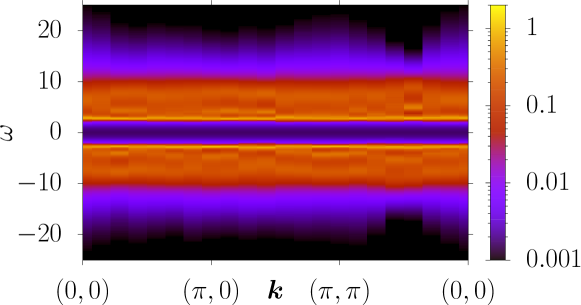
Figure 2: Single-particle spectral function $A(\bm{k},\omega)$ of the $c$-fermions at $t=0$. Here, $\beta=L=14$, $\omega_{0}=2.0$, $\tilde{g}=\sqrt{2/k}g=2$, $\lambda=0.5$.

In Fig. 2, we show the single-particle spectral function of the $c$ fermions at $t=0$, revealing a gap and the absence of dispersion. The single-particle gap corresponds to the energy difference between the low-lying $\hat{Q}_{i}$ sectors.

To capture the physics in this limit, we fractionalize the $c$ fermion into a $\mathbb{Z}_{2}$ matter field and an $f$ fermion[28],

$$\hat{c}^{\dagger}_{\bm{i},\sigma}=\hat{\tau}^{z}_{\bm{i}}\hat{f}^{\dagger}_{\bm{i},\sigma}$$ (18)

with the constraint

$$\hat{\tau}^{x}_{\bm{i}}\hat{p}_{\bm{i}}=1$$ (19)

and Pauli matrices $\hat{\tau}^{x}_{\bm{i}}$ and $\hat{\tau}^{z}_{\bm{i}}$. The constraint implies that the $\mathbb{Z}_{2}$ matter field, $\hat{\tau}^{z}_{\bm{i}}$, carries the $\mathbb{Z}_{2}$ charge and $\hat{f}^{\dagger}_{\bm{i},\sigma}$ the quantum numbers of the electron, namely, its global U(1) charge and spin. This is in contrast to Refs. [29, 30], where a gauge invariant (i.e., no $\mathbb{Z}_{2}$ charge) $c$ fermion is replaced by the product of a $\mathbb{Z}_{2}$-charged $f$ fermion and a slave spin.

In this representation, the Hamiltonian takes the form

$$\hat{H} = \frac{g}{\sqrt{2m\omega_{0}}}\sum_{b}\left(\hat{b}_{b}^{\dagger}+\hat{b}_{b}^{\phantom{\dagger}}\right)\hat{K}^{f}_{b}+\omega_{0}\sum_{b}\hat{b}_{b}^{\dagger}\hat{b}_{b}^{\phantom{\dagger}}$$ (20)

$$\quad-\lambda\sum_{b}\left(\hat{K}_{b}^{f}\right)^{2},$$

with

$$\hat{K}^{f}_{b}=\sum_{\sigma}\left(\hat{f}^{\dagger}_{\bm{i},\sigma}\hat{f}^{\phantom{\dagger}}_{\bm{j},\sigma}+\text{h.c.}\right),\,\,\hat{b}_{b}^{\dagger}=\hat{\tau}^{z}_{\bm{i}}\hat{a}_{b}^{\dagger}\hat{\tau}^{z}_{\bm{j}}$$ (21)

for $b=\left\langle\bm{i},\bm{j}\right\rangle$. The constraints can be written as

$$\hat{Q}_{\bm{i}}=\hat{\tau}^{x}_{\bm{i}}(-1)^{\sum_{\bm{\delta}}\hat{b}_{\langle\bm{i},\bm{i}+\bm{\delta}\rangle}^{\dagger}\hat{b}_{\langle\bm{i},\bm{i}+\bm{\delta}\rangle}^{\phantom{\dagger}}}\,.$$ (22)

Because $\hat{b}_{b}^{\dagger}$ and $\hat{f}^{\dagger}_{\bm{i},\sigma}$ carry no $\mathbb{Z}_{2}$ charge, they can propagate. In particular, $\hat{b}^{\dagger}$ can condense. The orthogonal fermion representation is a good starting point for mean-field theories.

II.3.4 Adiabatic limit $\omega_{0}\rightarrow 0$ at $t=0$

To discuss this limit, it is convenient to return to first quantization,

$$\hat{q}_{b}=\frac{1}{\sqrt{2m\omega_{0}}}\left(\hat{b}_{b}^{\dagger}+\hat{b}_{b}^{\phantom{\dagger}}\right)\,.$$ (23)

For $\omega_{0}\rightarrow 0$, Hamiltonian (20) becomes

$$\hat{H}=g\sum_{b}\hat{q}_{b}\hat{K}^{f}_{b}+\frac{k}{2}\sum_{b}\hat{q}_{b}^{2}-\lambda\sum_{b}\left(\hat{K}_{b}^{f}\right)^{2}\,.$$ (24)

Equation (24) has reflection positivity (see Ref. [31]) for any line P parallel to the lattice vectors and cutting through the center of the bonds. Thereby, the flux through a circuit with lattice sites corresponding to the corners of a plaquette will take the value $\pi$ [31]. A circuit is a set of lattice sites $i_{1},i_{2},\dots,i_{n},i_{1}$ with $q_{i_{m},i_{m+1}}\neq 0\,\,\forall m$. Hence, if all plaquettes turn out to define circuits, Lieb’s theorem [31] implies that the $f$ fermions acquire a Dirac spectrum.

II.3.5 Anti-adiabatic limit $\omega_{0}\rightarrow\infty$ at $t=0$

For $\omega_{0}\rightarrow\infty$ and $t=0$, Eq. (3) becomes equivalent to the model studied in Ref. [18], describing fermions coupled to quantum Ising spins. This can be seen by approximating the phonons as hard-core bosons with the constraint $(\hat{a}_{b}^{\dagger})^{2}=0$ and defining Ising variables

$$\hat{s}^{x}_{b}=2\hat{a}_{b}^{\dagger}\hat{a}_{b}^{\phantom{\dagger}}-1,\quad\hat{s}^{z}_{b}=\hat{a}_{b}^{\dagger}+\hat{a}_{b}^{\phantom{\dagger}}\,.$$ (25)

II.4 Previous work

Until recently, most investigations of the 2D SSH model (1) were based on mean-field treatments or the assumption of classical phonons ($\omega_{0}=0$). The focus was on the true VBS pattern in the ground state [32, 33, 34, 35], the possible existence of a multi-mode Peierls state with no well-defined ordering wavevector [36, 37, 38], and the emergence of AFM order from additional electron-electron repulsion [33, 39, 40, 41, 42]. These works were followed by unbiased QMC investigations on the honeycomb lattice [43], the Lieb lattice [44], and the square lattice considered here [22, 3, 4, 23, 24]. On the latter, a unique VBS ground state with ordering wavevector $(\pi,\pi)$—suggested by mean-field theory—is well established. Surprisingly, the SSH model also supports AFM order from electron-phonon coupling at sufficiently high phonon frequencies [3, 4].

III Method

We simulated the modified SSH model (3) using an auxiliary-field QMC approach. To decouple the electron-phonon interaction, we first rewrite the Hamiltonian to make the interaction term a perfect square,

$$\hat{H} = \hat{H}_{t}+\hat{H}_{\lambda}+\hat{H}_{\mathrm{ph}}$$ (26)

$$\hat{H}_{t} = -t\sum_{b}\hat{K}_{b}\,,\quad\hat{H}_{\lambda}=-\lambda\sum_{b}\left(\hat{K}_{b}-\frac{g}{2\lambda}\hat{X}_{b}\right)^{2}\,,$$

$$\hat{H}_{\omega_{0}} = \sum_{b}\frac{1}{2m}\hat{P}_{b}^{2}+\left(\frac{k}{2}+\frac{g^{2}}{4\lambda}\right)\hat{X}_{b}^{2}\,.$$

Using a Trotter decomposition with step size $\Delta\tau=\beta/L_{\tau}$, the partition function reads

$$Z = \mathop{\mathrm{Tr}}{e^{-\beta\hat{H}}}=\mathop{\mathrm{Tr}}{\left[\left(e^{-\Delta\tau\hat{H}}\right)^{L_{\tau}}\right]}$$

$$e^{-\Delta\tau\hat{H}} = e^{-\frac{\Delta\tau}{2}\hat{H}_{t}}\left(\prod_{b=1}^{N_{\text{b}}}e^{-\frac{\Delta\tau}{2}\hat{H}_{\lambda,b}}\right)e^{-\Delta\tau\hat{H}_{\omega_{0}}}$$

$$\times\left(\prod_{b=N_{\text{b}}}^{1}e^{-\frac{\Delta\tau}{2}\hat{H}_{\lambda,b}}\right)e^{-\frac{\Delta\tau}{2}\hat{H}_{t}}+\mathcal{O}(\Delta\tau^{3})\,$$

with $N_{\text{b}}=2N_{\text{s}}$ the total number of bonds and $\beta=1/T$ the inverse temperature. To preserve the hermiticity of the Hamiltonian, we used a symmetric Trotter decomposition [14, 45]. In Appendix A, we compare this decomposition with an asymmetric one that breaks the hermiticity. Electrons and phonons can now be decoupled with a discrete Hubbard-Stratonovich transformation [46, 47, 48, 17],

$$e^{\frac{\lambda\Delta\tau}{2}\left(\hat{K}_{b}-\frac{g}{2\lambda}\hat{X}_{b}\right)^{2}}=$$ (28)

$$\frac{1}{4}\sum_{l=\pm 1,\pm 2}\gamma(l)e^{\sqrt{\frac{\Delta\tau\lambda}{2}}\eta(l)\left(\hat{K}_{b}-\frac{g}{2\lambda}\hat{X}_{b}\right)}+\mathcal{O}((\Delta\tau\lambda)^{4})\,,$$

where

$$\gamma(\pm 1)=1+\sqrt{6}/3\,,\quad\eta(\pm 1)=\pm\sqrt{2\left(3-\sqrt{6}\right)}\,,$$ (29)

$$\gamma(\pm 2)=1-\sqrt{6}/3\,,\quad\eta(\pm 2)=\pm\sqrt{2\left(3+\sqrt{6}\right)}\,.$$

Since the Trotter decomposition introduces a systematic error of order $\Delta\tau^{3}$ [49], we can assume the Hubbard-Stratonovich transformation to be exact. To evaluate the trace over the phonons in the partition function we use a path integral in real-space representation with the eigenstates $|x_{b}\rangle$ and eigenvalues $X_{b}$ of the position operator,

$$Z = \sum_{\left\{l_{b,\tau,\alpha}\right\}}\left(\prod_{b,\tau,\alpha}\frac{\gamma(l_{b,\tau,\alpha})}{4}\right)\det\left[1+B(\beta,0)\right]$$

$$\quad\times\int\prod_{b,\tau}dX_{b,\tau}e^{-\sum_{b}\bm{X}_{b}^{\mathrm{T}}A\bm{X}_{b}-\sum_{b}\bm{v}_{b}^{\mathrm{T}}\bm{X}_{b}}\,,$$

where we used

$$\bm{X}_{b}^{\mathrm{T}} = \left(X_{b,1},X_{b,2},\dots,X_{b,N_{\tau}}\right)\,,$$ (31)

$$v_{b,\tau} = g\sqrt{\frac{\Delta\tau}{8\lambda}}\left(\eta(l_{b,\tau,2})+\eta(l_{b,\tau-1,1})\right)\,,$$

$$A_{k,l} = \Delta\tau\left(\alpha\delta_{k,l}-\gamma\left(\delta_{k,l+1}+\delta_{k,l-1}\right)\right)\,,$$

$$\alpha = \frac{k}{2}+\frac{g^{2}}{4\lambda}+\frac{m}{\Delta\tau^{2}}\,,\quad\gamma=\frac{m}{2\Delta\tau^{2}}\,.$$

The index $\alpha=1,2$ is needed as the symmetric Trotter decomposition produces two Hubbard-Stratonovich decompositions per time slice and bond. For the electronic part, we rewrite the trace as a determinant [13],

$$B(\tau_{1},\tau_{2}) = \prod_{\tau=\tau_{2}+\Delta\tau}^{\tau_{1}}e^{\frac{\Delta\tau}{2}t\sum_{b}K_{b}}\left(\prod_{b=1}^{N_{\text{b}}}e^{\sqrt{\frac{\Delta\tau\lambda}{2}}\eta(l_{b,\tau,1})K_{b}}\right)$$ (32)

$$\times\left(\prod_{b=N_{\text{b}}}^{1}e^{\sqrt{\frac{\Delta\tau\lambda}{2}}\eta(l_{b,\tau,2})K_{b}}\right)e^{\frac{\Delta\tau}{2}t\sum_{b}K_{b}}\,.$$

We can interpret the matrix $A$ as a tight-binding Hamiltonian on a periodic chain with $L_{\tau}$ sites, hopping $\alpha$, and on-site potential $\gamma$. The eigenvalues of $A$ are

$$a_{n}=\Delta\tau\left(\alpha-2\gamma\cos\nu_{n}\right)=\frac{k}{2}+\frac{g^{2}}{4\lambda}+\frac{m}{\Delta\tau^{2}}(1-\cos\nu_{n})\,,$$ (33)

with $\nu_{n}=\frac{2\pi}{L_{\tau}}n$ and $1\leq n\leq L_{\tau}$. The matrix $A$ is positive definite for the whole parameter range and we can integrate out the phonons to obtain

$$Z \propto \sum_{\left\{l_{b,\tau,\alpha}\right\}}\left(\prod_{b,\tau,\alpha}\gamma(l_{b,\tau,\alpha})\right)$$

$$\quad\times\exp{\left\{\frac{1}{4}\sum_{b}\bm{v}_{b}^{\mathrm{T}}A^{-1}\bm{v}_{b}\right\}}\det\left[1+B(\beta,0)\right]\,.$$

The summation over the auxiliary fields $\{l_{b,\tau,\alpha}\}$ is done stochastically with QMC methods employing single-spin-flip and global updates, which are accepted according to the Metropolis-Hastings algorithm [50, 51]. For the global updates, we randomly choose a rectangular section of auxiliary fields in the (2+1)D configuration space and swap it with a rectangle of the same size but displaced by $L_{\tau}/2$ in the imaginary-time direction.

Additionally, we used a $\beta$-doubling method to reduce warm-up times. We started by running a simulation with a given parameter set for some time with an inverse temperature $\beta_{1}$ smaller than the final value $\beta$. Then, we used the last configuration of this run as a starting configuration for a simulation with a higher inverse temperature $\beta_{2}$, $\beta_{1}<\beta_{2}\leq 2\beta_{1}$, identifying $\eta(l_{b,\tau+\beta_{1},\alpha})=\eta(l_{b,\tau,\alpha})$ at the beginning. After two or three such steps, we reached the final inverse temperature $\beta$.

Appendix B contains a comparison of the method described here and used for the results with two other methods that do not involve integrating out the phonons. For the parameters considered, the present approach provides a substantial speedup.

IV Results

For the simulations, we absorbed $k$ into a renormalization of the phonon fields, $\tilde{x}_{b,\tau}=\sqrt{{k}/{2}}x_{b,\tau}$, and set $\tilde{g}=\sqrt{2/k}g=2$, $\lambda=0.5$, as well as $\Delta\tau=0.05$.

To detect the various phases, we measured imaginary-time-displaced correlation functions

$$\left[S_{O}(\bm{q},\tau)\right]_{\mu,\nu}=\left\langle\hat{O}_{\mu}(\bm{q},\tau)\hat{O}_{\nu}(-\bm{q})\right\rangle-\left\langle\hat{O}_{\mu}(\bm{q})\right\rangle\left\langle\hat{O}_{\nu}(-\bm{q})\right\rangle$$ (35)

and corresponding susceptibilities,

$$\chi_{O}(\bm{q})=\int_{0}^{\beta}d\tau \mathop{\mathrm{Tr}}S_{O}(\bm{q},\tau)\,,$$ (36)

for several observables $\hat{O}$. The notation is general enough for correlators with a matrix structure; the scalar case is obtained by dropping the indices $\mu,\nu$. Here, $\bm{q}$ is a wave vector inside the first Brillouin zone.

Because of the O(4) symmetry of Hamiltonian (3), the spin correlator is degenerate with charge and s-wave superconducting correlation functions, see Sec. II.2. Therefore, we focus on the $z$-component of spin,

$$\hat{S}^{z}(\bm{q})=\frac{1}{\sqrt{N_{\text{s}}}}\sum_{\bm{i}}e^{i\bm{q}\cdot\bm{i}}\left(\hat{n}_{\bm{i},\uparrow}-\hat{n}_{\bm{i},\downarrow}\right)\,.$$ (37)

To detect the breaking of particle-hole symmetry, we measured correlation functions of the parity $\hat{p}_{\bm{i}}$ [Eq. (5)]. Additionally, we calculated dimer correlations to detect VBS order that breaks the discrete $C_{4}$ symmetry of the square lattice,

$$\hat{\Delta}_{\mu}(\bm{q}) = \frac{1}{\sqrt{N_{\text{s}}}}\sum_{\bm{i}}e^{i\bm{q}\cdot\bm{i}}\hat{\Delta}_{\bm{i},\mu}\,,$$ (38)

$$\hat{\Delta}_{\bm{i},\mu} = \hat{S}_{\sigma,\rho}(\bm{i})\hat{S}_{\rho,\sigma}(\bm{i}+\bm{a}_{\mu})\,,$$

where

$$\hat{S}_{\sigma,\rho}(\bm{i})=\hat{c}^{\dagger}_{\bm{i},\sigma}\hat{c}^{\phantom{\dagger}}_{\bm{i},\rho}-\frac{1}{2}\delta_{\sigma,\rho}\,.$$ (39)

The vectors $\bm{a}_{x}^{\mathrm{T}}=(1,0)$ and $\bm{a}_{y}^{\mathrm{T}}=(0,1)$ connect site $\bm{i}$ to its nearest neighbors and $\mu\in\{x,y\}$.

We further present results for the correlation ratios

$$R_{S,O}=1-\frac{\mathop{\mathrm{Tr}}S_{O}(\bm{q}_{O}+\Delta\bm{q})}{\mathop{\mathrm{Tr}}S_{O}(\bm{q}_{O})}\,,$$ (40)

where $|\Delta\bm{q}|=2\pi/L$ is the shortest wave vector on an $L\times L$ lattice and $\bm{q}_{O}$ the ordering wave vector of observable $O$. The correlation ratio is a renormalization group invariant quantity and takes on values close to zero/one in the disordered/ordered phase. For the susceptibilities, correlation ratios can be defined analogously.

The single-particle spectral function $A(\bm{k},\omega)$, accessible in angular-resolved photoemission, was calculated from the imaginary-time Greens function with the stochastic maximum entropy method [52, 53] via

$$\langle\hat{c}^{\phantom{\dagger}}_{\bm{k},\sigma}(\tau)\hat{c}^{\dagger}_{\bm{k},\sigma}(0)\rangle=\frac{1}{\pi}\int\text{d}\omega\,\frac{e^{-\tau\omega}}{1+e^{-\beta\omega}}A(\bm{k},\omega)\,.$$ (41)

The dynamical structure factors for spins and dimers were computed from

$$\mathop{\mathrm{Tr}}S_{O}(\bm{q},\omega)=\frac{\mathop{\mathrm{Tr}}\chi^{\prime\prime}_{O}(\bm{q},\omega)}{1-e^{-\beta\omega}}\,,$$ (42)

where the imaginary part of the dynamical susceptibility was obtained by inverting

$$\mathop{\mathrm{Tr}}S_{O}(\bm{q},\tau)=\frac{1}{\pi}\int d\omega\frac{e^{-\tau\omega}}{1-e^{-\beta\omega}}\mathop{\mathrm{Tr}}\chi^{\prime\prime}_{O}(\bm{q},\omega)$$ (43)

with the maximum entropy method [17].

Finally, we also measured observables that depend on phonon variables, such as the flux operator $\hat{\Phi}_{\bm{i}}$. The latter is defined as the product over the effective hoppings on the bonds $b$ of an elementary plaquette $\Box_{\bm{i}}$,

$$\hat{\Phi}_{\bm{i}}=\prod_{b\in\Box_{\bm{i}}}\left(-t+g\hat{X}_{b}\right)\,,$$ (44)

where $\bm{i}$ is one of the four corner sites of a plaquette. Because the phonons were integrated out, such observables are not directly accessible but require a source term in the action, as discussed in Appendix C.

IV.1 Dynamically generated $\pi$-flux

We first consider the flux per elementary plaquette [Eq. (44)] in the $t$-$\omega_{0}$ plane, shown in Fig. 3. In an electron-phonon context, $g\hat{X}_{b}$ in Eq. (3) should be a small perturbation to the bare hopping $t$. Hence, in this regime, the flux per plaquette is positive. The $\hat{c}^{\dagger}_{\bm{i},\sigma}$ operators create electrons and the hopping matrix element leads to a $(\pi,\pi)$-nested Fermi surface. The latter gives rise to instabilities at $\bm{q}=\bm{M}$. Possible orderings include an AFM phase or a $(\pi,\pi)$ VBS phase, as observed for $\lambda=0$ [22, 3, 4, 23, 24].

In the opposite, phonon-assisted hopping limit (i.e., at $t=0$), our model reduces to an unconstrained $\mathbb{Z}_{2}$ gauge theory, see Sec. II.3.3. The $c$ fermions acquire a locally conserved $\mathbb{Z}_{2}$ charge and cannot propagate in space, as demonstrated in Fig. 2. However, gauge invariant quantities such as the local spin or local charge can propagate. Hence, the $c$ fermion corresponds to a so-called orthogonal fermion [54]. To understand the single-particle physics, we have to adopt the $f$ fermions [Eq. 18)]. The latter carry no locally conserved $\mathbb{Z}_{2}$ charge, can hop from site to site, and acquire a phase of $0$ or $\pi$ when circulating around a plaquette. A phase of $\pi$ is favored by Lieb’s theorem [31] and confirmed by the numerical results in Fig. 3.

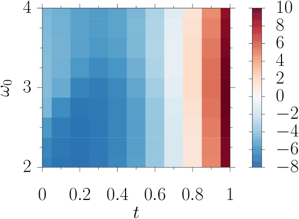
Figure 3: Average flux per plaquette $\frac{1}{N_{\text{s}}}\sum_{\bm{i}}\langle\hat{\Phi}_{\bm{i}}\rangle$ for $\beta=L=8$.

The generated $\pi$-fluxes cause the $f$ fermions to acquire a Dirac dispersion relation , which has important consequences for the understanding of the phase diagram. In particular, we can classify the interaction-generated ordered states in terms of mass terms that generate a single-particle gap and break discrete or continuous symmetries [56]. Of particular importance are the two $(\pi,0)$ VBS masses and the three AFM mass terms, which break the $\mathrm{C}_{4}$ lattice symmetry and the $\mathrm{SU}(2)$ spin symmetry, respectively. The Dirac vacuum allows for topological terms in the action, which play a key role in the understanding of DQCPs [57, 58, 21].

Our symmetry arguments are valid only at $t=0$. Beyond this limit, $\hat{Q}_{\bm{i}}$ is not a good quantum number and the $\mathbb{Z}_{2}$ charge is not locally conserved. As a consequence, the $c$ fermions acquire a dispersion, albeit small for small $t$. This is visible from the single-particle spectral functions in Figs. 6(Ia)-(Ie). The lack of dispersion of the $c$ fermions for small values of $t$ suggests that it is still appropriate to work in the $f$ basis. The hopping of the $f$ fermions reads

$$\sum_{b=\langle\bm{i},\bm{j}\rangle}\hat{\tau}^{z}_{i}\left(-t+g\hat{X}_{b}\right)\hat{\tau}^{z}_{j}\hat{K}^{f}_{b}.$$ (45)

Since $\left(\hat{\tau}^{z}_{i}\right)^{2}=1$, the flux $\hat{\Phi}_{\bm{i}}$, [Eq. (44)] shown in Fig. 3 indeed corresponds to the flux acting on the $f$ fermions. In Sec. IV.3, we will further argue that the free energy is an analytical function of $t$ at $t=0$, so that the $t=0$ physics is adiabatically connected to a region around $t=0$ set by the convergence radius of the series.

As a function of $t$, Fig. 3 reveals a crossover where the flux changes sign. To a first approximation, this sign change does not depend on $\omega_{0}$. As we will see below, it marks the crossover between a regime that can be understood in terms of the $f$ fermions with a Dirac dispersion and a regime of $c$ fermions with a nested Fermi surface.

IV.2 Deconfined quantum critical point

Next, we study a cut along the frequency axis at a small but finite $t=0.1$ that explicitly breaks the local $\mathbb{Z}_{2}$ symmetry. Figure 4(a) shows the average flux per plaquette as a function of system size and phonon frequency. The flux stays negative irrespective of $\omega_{0}$, corresponding to a dynamically generated $\pi$-flux in each plaquette. The choice $\beta=L$ in the finite-size scaling is motivated by the Dirac band structure of the $f$ fermions, as discussed below. The pronounced change of the flux around $\omega_{0}\approx 2.7$ suggests the possibility of a phase transition.

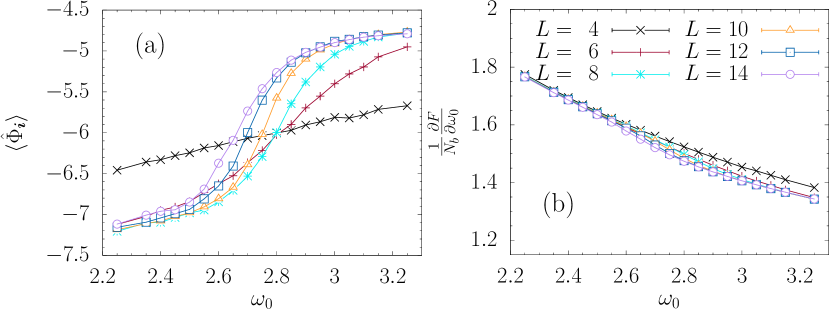
Figure 4: Flux and normalized free-energy derivative with respect to $\omega_{0}$. Here, $t=0.1$, $\beta=L$.

Another observable that carries information about a possible phase transition is the free energy $F$. At a fixed electronic hopping $t$, its first derivative with respect to $\omega_{0}$ is given by

$$\frac{\partial F}{\partial\omega_{0}}=m\omega_{0}\sum_{b}\langle\hat{X}_{b}^{2}\rangle-\frac{g}{2\omega_{0}}\sum_{b}\langle\hat{K}_{b}\hat{X}_{b}\rangle\,.$$ (46)

Figure 4(b) reports results for this quantity as a function of $\omega_{0}$ and for different $L$. The data reveal no jumps or kinks on the scale considered, essentially ruling out a strongly first-order transition.

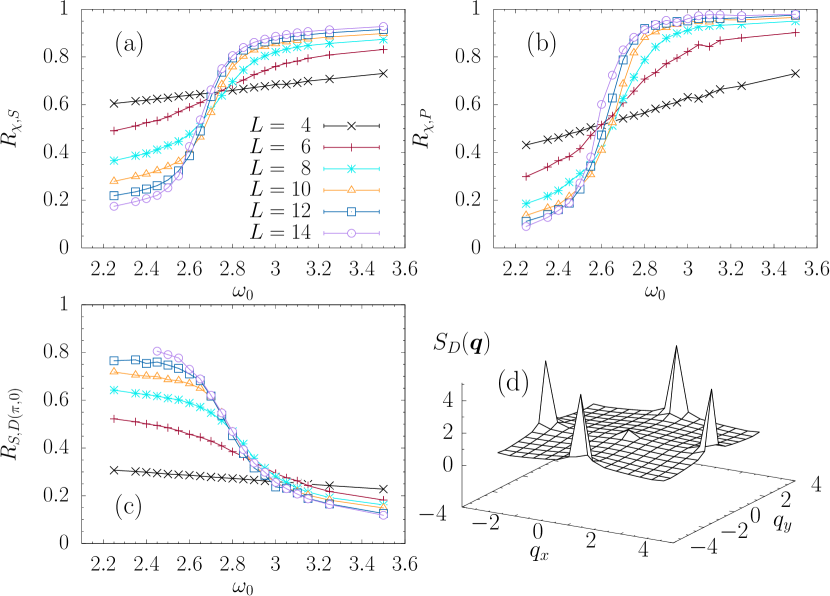
Figure 5: Susceptibility correlation ratios for (a) spin at $\bm{M}$, (b) parity at $\bm{\Gamma}$, and (c) dimers at $\bm{X}$ as a function of $\omega_{0}$ for $\beta=L$. (d) Equal-time dimer correlation function in the first Brillouin zone for $\beta=L=14$, $\omega_{0}=2.25$. Here, $t=0.1$.

In Figs. 5(a)-(c), we present the correlation ratios of the spin and parity susceptibilities as well as the equal-time dimer correlation function. The correlation ratio scales as

$$R_{\chi,O}=f\left(L^{z}/\beta,[\omega_{0}-\omega_{0}^{c}]L^{1/\nu}\right)\,,$$ (47)

with the dynamical exponent $z$ and the correlation length exponent $\nu$. Here, we neglect corrections to scaling that will cause a meandering of the crossing points with increasing $L$. Unless indicated otherwise, we used $\beta=L$ when measuring correlation ratios. This choice appears to be justified by the dynamical dimer structure factor [Fig. 6(IId)] and the dynamical spin structure factor [Fig. 6(IIId)] close to the presumed critical point. Both quantities are consistent with a linear dispersion relation around the ordering wave vector and hence with an exponent $z=1$. Furthermore, we note that mass terms in the Dirac equation do not break Lorentz symmetry so that this scaling remains justified even in the ordered phases.

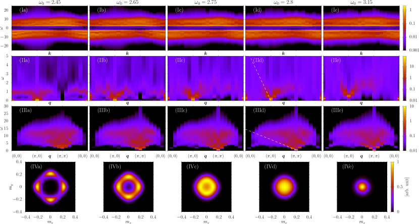
Figure 6: (Ia)-(Ie) Single-particle spectral function $A(\bm{k},\omega)$, (IIa)-(IIe) dynamical VBS structure factor $S_{D}(\bm{q},\omega)$, (IIIa)-(IIIe) dynamical spin structure factor $S_{S}(\bm{q},\omega)$, and (IVa)-(IVe) histogram of the VBS order parameter $m_{x}$ and $m_{y}$ for different $\omega_{0}$ and $t=0.1$, $\beta=L=14$. White dashed lines in panels (IId) and (IIId) are guides to the eye.

The spin correlation ratio $R_{\chi,S}$ at wave vector $\bm{M}$ [Fig. 5(a)] reveals long-range AFM order at high phonon frequencies. Simultaneously, the parity correlation ratio shows ordering at $\bm{\Gamma}=(0,0)$. By lowering $\omega_{0}$, AFM order disappears but dimer correlations exhibit a marked increase. The equal-time dimer correlation function is dominated by four peaks at $\bm{q}=(\pi,0)$ and equivalent wave vectors [Fig. 5(d)]. The corresponding correlation ratio at $\bm{X}$ increases with decreasing $\omega_{0}$ [Fig. 5(c)].

The correlation ratios are consistent with a phase transition from an AFM state at high phonon frequencies to a $(\pi,0)$ VBS state at $\omega_{0}^{c}\approx 2.7$, even though finite-size effects make a more quantitative analysis difficult. Regarding the nature of this phase transition, several possible explanations exist. We cannot exclude a weakly first-order transition. The data are also consistent with an intermediate coexistence region, especially since the quality of the results for the dimer correlation ratio is limited by long autocorrelation times. A third possibility is a direct second-order transition. Because the AFM and VBS phases break different symmetries, such a transition falls outside the Ginzburg-Landau paradigm and is instead a candidate for a deconfined quantum critical point [59, 6]. We will favor the latter possibility in the remainder of this article.

Let us now turn to the spin, VBS, and $c$-fermion spectral functions, starting with theoretical expectations in the limit $t=0$. Because the VBS and spin order parameters carry no $\mathbb{Z}_{2}$ charge, they will exhibit dispersive features even for $t=0$. In contrast, the $c$ fermion has a $\mathbb{Z}_{2}$ charge and the corresponding spectral function $A(\bm{k},\omega)=A(\omega)$, as shown in Fig. 2. At $t=0$, the Hamiltonian is block diagonal in $\hat{Q}_{\bm{i}}$, which is a good quantum number. Since $\hat{c}^{\dagger}_{\bm{i},\sigma}$ generates a $\mathbb{Z}_{2}$ charge, it causes changes between different $\hat{Q}_{\bm{i}}$ sectors. Hence, the single-particle gap can be understood in terms of the energy difference between different $\hat{Q}_{\bm{i}}$ sectors. States such as a Dirac spin liquids, or orthogonal semi-metals [54, 18, 60] would exhibit gapless excitations in the spin sector, but gapped excitations in the single-particle spectral function. Hence, there is à priori no relation between the gaps observed in the spin and the $c$-fermion sectors.

Signatures of our theoretical expectations for $t=0.0$ are apparent in Fig. 6, obtained for $t=0.1$. As for the case of $t=0$ shown in Fig. 2, the spectral function is essentially independent of $\bm{k}$ in Figs. 6(Ia)-(Ie). Moreover, the dominant features show very little dependence on $\omega_{0}$, with substantial spectral weight at $\Delta_{\text{sp}}\simeq 2.5$. In the VBS phase at $\omega_{0}=2.45$ [Fig. 6(IIIa)], the dynamical spin structure factor is reminiscent of gapped Dirac fermions due to the onset of VBS order. The spin gap can be read off as $\Delta_{\text{s}}\simeq 2.5$. Since $t>0$ violates the local $\mathbb{Z}_{2}$ symmetry, a spin wave can decay into two $c$ fermions. The fact that $\Delta_{\text{s}}<2\Delta_{\text{sp}}$ reflects vertex corrections accounting for electron-hole binding.

For $\omega_{0}=2.45$, we have VBS order that breaks the $C_{4}$ lattice symmetry. The VBS spectral function in Fig. 6(IIa) shows a sharp mode at $\omega=0$ and at the ordering wave vector $\bm{q}=(\pi,0)$ that accounts for the Bragg peak associated with this order. In Fig. 6(IVa), we show the histogram of the VBS order parameter with $m_{\mu}=\hat{\Delta}_{\mu}(\bm{q}_{\mu})/\sqrt{N_{s}}$, $\mu=x,y$, $\bm{q}_{x}=(\pi,0)$, and $\bm{q}_{y}=(0,\pi)$. . We find four peaks along the $x$ and $y$ axes, reflecting the four-fold degeneracy of the $(\pi,0)$ VBS order parameter.

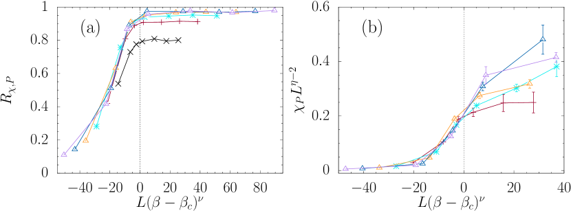
Figure 7: Data collapse of (a) the parity susceptibility correlation ratio and (b) the parity susceptibility using 2D Ising exponents ($\nu=1$, $\eta=1/4$). Here, $\bm{q}=\bm{\Gamma}$, $t=0.1$, $\omega_{0}=3.5$.

It is beyond the scope of this work to study the critical exponents of the purported DQCP. However, DQCPs have a number of hallmark signatures that can be detected in the dynamical responses. First, at criticality, the $\mathrm{C}_{4}$ lattice symmetry is enlarged to U(1). This symmetry enhancement is captured by $S_{D}(\bm{q},\omega)$ in the form of a spectrum with a linear mode. Comparing Fig. 6(IIa) (deep in the VBS phase) to Fig. 6(IId) (close to the DQCP), we recognize that the Bragg peak evolves towards a spectrum with a linear dispersion relation. The dashed line in Fig. 6(IId) is a guide to the eye that indicates the velocity of this mode. Equivalently, the histograms of Fig. 6(IVa)-(IVd) reveal that the four-peak structure evolves to a circle upon approaching the critical point. Similar phenomena have been observed in Ref. [62].

Another DQCP hallmark is a single, continuous and direct transition with emergent Lorentz symmetry. The corresponding theory has a single velocity. Our data are consistent with this expectation: at criticality, the U(1) velocity in Fig. 6(IId) compares favorably with the spin velocity in Fig. 6(IIId). Hence, several of the defining properties of the DQCP are borne out by our results.

In the AFM phase, Figs. 6(IIe) and (IVe), we observe a gap in the dimer correlations, a Goldstone mode in the spin correlations, and a single central peak in the histogram.

In contrast to models of DQCPs with $\mathrm{SU}(2)\times\mathrm{C}_{4}$ [62] or $\mathrm{SU}(2)\times\mathrm{U}(1)$ symmetry [63], our model has an $\mathrm{O}(4)\times\mathrm{C}_{4}$ symmetry. In the AFM phase, the symmetry is broken down to $\mathrm{U}(1)\times\mathrm{C}_{4}$. As we will argue below, this symmetry reduction occurs in two steps. The parity being a $\mathbb{Z}_{2}$ order parameter, we expect a finite temperature 2D Ising phase transition with exponents $\nu=1$ and $\eta=1/4$. These exponents yield a satisfactory data collapse of the parity correlation ratio and susceptibility in Fig. 7. The collapse of the correlation ratio yields a critical inverse temperature of $\beta_{c}\simeq 5.6$, whereas the susceptibility data gives $\beta_{c}\simeq 5.4$. Below the finite temperature Ising transition, the symmetry is reduced to $\mathrm{SU}(2)\times\mathrm{SU}(2)$ and either the odd or even parity sector is spontaneously selected. Only at $T=0$ is the continuous SU(2) symmetry broken down to U(1).

IV.3 From assisted hopping to phonon-modulated direct hopping

So far, we have focused on the small-$t$ regime of the phase diagram, where the physics can be understood in terms of the $f$ fermions with an underlying Dirac dispersion stemming from dynamically generated $\pi$-fluxes. We now vary $t$, and thereby the ratio of direct to phonon-assisted hopping, at a fixed phonon frequency $\omega_{0}=2.0$.

Figure 8: Flux and normalized free-energy derivative with respect to $t$. Here, $\omega_{0}=2.0$, $\beta=L$.

As previously revealed by Figs. 1 and 3, the flux changes its sign as a function of $t$. In Fig. 8(a), we present results for the flux for different lattice sizes. It varies smoothly, with the sign changing at $t\approx 0.75$. Starting from large values of $t$, the flux decreases until it reaches a minimum at $t\approx 0.2$ followed by a slight increase.

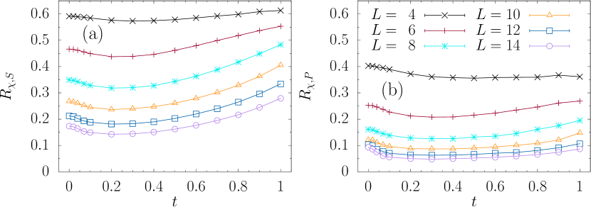
Figure 9: Susceptibility correlation ratios for (a) spin at $\bm{M}$ and (b) parity at $\bm{\Gamma}$. Here, $\omega_{0}=2.0$, $\beta=L$.

The derivative of the free energy with respect to $t$ is given by the average kinetic energy

$$\frac{\partial F}{\partial t}=-\sum_{b}\langle\hat{K}_{b}\rangle\,.$$ (48)

Results are shown in Fig. 8(b). At $t=0$, where the model has the local $\mathbb{Z}_{2}$ symmetry, the kinetic energy vanishes by symmetry and only phonon-mediated hopping takes place. We can expand the free energy around $t=0$,

$$F(t)=F_{0}-t^{2}\int_{0}^{\beta}d\tau\sum_{b}\langle\hat{K}_{b}(\tau)\hat{K}_{b}(0)\rangle_{0}+{\cal O}(t^{4})$$ (49)

with $F_{0}$ the free energy at $t=0$ and $\langle\hat{O}\rangle_{0}$ the expectation value of an observable $\hat{O}$ with respect to the Hamiltonian with $t=0$. Here, only even powers occur since $F(t)=F(-t)$. Hence, ${\partial F}/{\partial t}=-2t\int_{0}^{\beta}d\tau\sum_{b}\langle\hat{K}_{b}(\tau)\hat{K}_{b}(0)\rangle_{0}+{\cal O}(t^{3})$. Since the time-displaced correlation function is positive, ${\partial F}/{\partial t}$ decreases linearly with $t$ for small $t$. This is consistent with the QMC data. Within the numerical resolution and for our choice of $\beta=L$, ${\partial F}/{\partial t}$ is smooth as a function of $t$. As mentioned above, the analytical behavior of the free energy around $t=0$ implies that the physics at small $t>0$ is adiabatically connected to that at $t=0$.

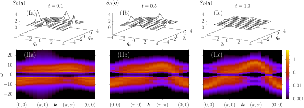
Figure 10: (Ia)-(Ic) Equal-time dimer correlation function in the first Brillouin zone for $\beta=L=10$. (IIa)-(IIc) Single-particle spectral function $A(\bm{k},\omega)$ for $\beta=L=14$. Here, $\omega_{0}=2.0$.

The results for the correlation ratios based on the spin and parity susceptibilities in Fig. 9 indicate the absence of spin order for all values of $t$ considered. In Figs. 10(Ia)-(Ic), we present the dimer correlation function for $t=0.1$, 0.5, and 1.0. For small $t$, where $\pi$-fluxes are dynamically generated, the system is in the $(\pi,0)$ VBS phase. When the hopping is increased, the dominant peaks at $(\pi,0)$ and equivalent wave vectors start to decrease and the VBS order melts. At $t=1.0$, the correlation function is almost flat.

Although VBS order is suppressed with increasing $t$, the single-particle gap remains open, as visible from the single-particle spectral function in Figs. 10(IIa)-(IIc). The latter evolves toward a cosine band structure. The band width is determined by an effective hopping $t_{\mathrm{eff}}=t-({g}/{N_{\text{b}}})\sum_{b}\langle\hat{X}_{b}\rangle$ due to the coupling to the phonons. At $t=1.0$ and $\omega_{0}=2.0$, we obtain $t_{\mathrm{eff}}=2.25$.

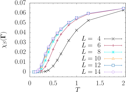
Figure 11: Spin susceptibility $\chi_{S}(\bm{\Gamma})$ as a function of temperature. Here, $t=1.0$, $\omega_{0}=2.0$.

The pseudogap phase at $t=1$ corresponds to an O(4) symmetric finite-temperature phase. Furthermore, the uniform spin susceptibility in Fig. 11 supports the existence of a finite spin gap. We understand this phase in terms of preformed pairs that will order at lower temperature. At $t=1$, a $\pi$-flux is absent and the $f$ fermion picture introduced above is no longer valid. Instead, we interpret the results in terms of an instability of an underlying $(\pi,\pi)$-nested Fermi surface. In this case, and at the mean-field level that becomes exact in the adiabatic limit, the transition temperature will follow an essential singularity. Hence, for our choice $\beta=L$, we expect to be above the expected transition temperature, limiting our ability to draw conclusions about the ground state. Strictly speaking, a $\beta=L$ scaling (i.e., $z=1$) is no longer justified in the absence of dynamically generated $\pi$ fluxes. Using lower temperatures within the present algorithm is challenging in this parameter region due to long autocorrelation times. While it is unclear from the present data which ordering wave vector is picked up for $T\to 0$ at large $t$, previous studies [22, 3, 4, 23, 24] suggest a $(\pi,\pi)$-ordered VBS ground state.

IV.4 Flux crossover within the AFM phase

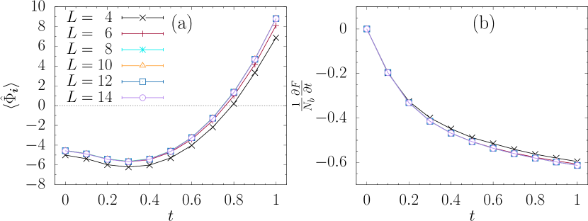
Figure 12: Flux and free-energy derivative with respect to $t$. Here, $\omega_{0}=4$, $\beta=L$.

In this section, we consider a value $\omega_{0}=4.0$, for which the system is in the AFM phase according to Fig. 1. AFM order is revealed by the correlation ratios in Fig. 13 for the entire range of hoppings considered, $0\leq t\leq 1$. Specifically, long-range order is visible at wave vector $\bm{M}$ in the spin sector [Fig. 13(a)] and at $\bm{q}=\bm{\Gamma}$ in the parity sector [Fig. 13(b)]. In contrast, the equal-time dimer correlation ratio excludes the presence of VBS order at $\bm{M}$ and $\bm{X}$ [Figs. 13(c)-(d)]. We note that the AFM phase corresponds to a Lorentz invariant phase, so that irrespective of a plaquette flux, the adopted $\beta=L$ scaling suffices to capture ground-state properties.

Results for the flux as a function of $t$ [Fig. 12(a)] are qualitatively very similar to those for $\omega_{0}=2.0$ [Fig. 8(a)]. The flux and the derivative of the free energy with respect to $t$ are smooth at the considered resolution of $t$, see Fig. 12(b). Comparison of Fig. 8(b) and Fig. 12(b) reveals that the slope of ${\partial F}/{\partial t}$, $\int_{0}^{\beta}d\tau\sum_{b}\langle\hat{K}_{b}(\tau)\hat{K}_{b}(0)\rangle_{0}$, is reduced for $\omega_{0}=4.0$. This is a consequence of the increased gap between different $\hat{Q}_{\bm{i}}$ sectors.

A pure $\mathbb{Z}_{2}$ lattice gauge theory supports deconfined and confined phases separated by an Ising transition at which fluxes (i.e., visons) proliferate [64, 65, 66]. In the AFM phase, the fermions are bound in particle-hole pairs that carry no $\mathbb{Z}_{2}$ charge. Hence, the AFM and gauge fluctuations effectively decouple at low energies, and two AFM phases are possible. The gauge field is deconfined in the AFM* phase but confined in the AFM phase. Such transitions have been discussed in Refs. [60, 20].

Because the hopping $t$ explicitly breaks the $\mathbb{Z}_{2}$ symmetry in our case, the AFM* and AFM phases cannot be strictly distinguished in the sense that they are separated by a critical point. Nevertheless, we understand the sign change in the flux in terms of a proliferation of visons and our data in terms of an AFM* to AFM crossover.

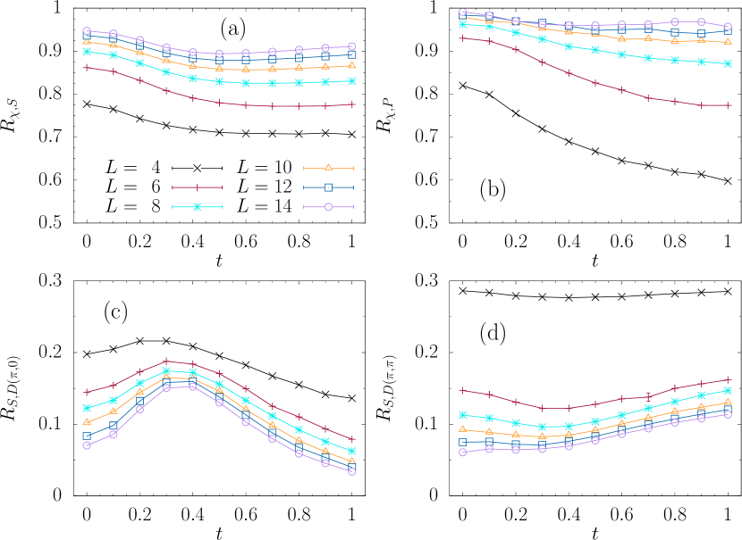
Figure 13: Correlation ratio of (a) the spin susceptibility at $\bm{M}$, (b) the parity susceptibility at $\bm{\Gamma}$, (c) dimer correlations at $\bm{X}$, (d) dimer correlations at $\bm{M}$. Here, $\omega_{0}=4.0$, $\beta=L$.

V Discussion and Conclusions

We studied a modified SSH model on a square lattice using an auxiliary-field QMC approach inspired by Ref. [12]. By adding a symmetry-allowed electronic interaction, we were able to integrate out the phonon degrees of freedom in the whole parameter space. This results in imaginary-time correlations between discrete auxiliary fields, which we sample with a combination of sequential single-spin-flip and global updates. In Appendix B, we argue that this discrete field approach is more efficient than updating the continuous phonon fields. With this method, we were able to study the phase diagram of the model as a function of the phonon frequency and the hopping strength.

In the original electron-phonon context of the SSH model, the ratio of phonon-assisted hopping to direct hopping has to be small [5]. However, allowing more general values of the hopping strength provides a direct route between a model with dominant direct hopping and a model with dominant phonon-assisted hopping. In the limiting case $t=0$, the symmetry of the model is enhanced by a local $\mathbb{Z}_{2}$ symmetry and it maps on an unconstrained lattice gauge theory. For any value of $t$, the model has a global O(4) symmetry. As a result, an AFM phase is degenerate with CDW and SC phases, and a partial particle-hole transformation maps the three AFM order parameters onto one CDW an two SC order parameters. These symmetries are also present in the SSH model without the extra term.

The limit $t=0$ is special due to the local $\mathbb{Z}_{2}$ symmetry. However, since the free energy is not singular, the physics of $t=0$ is representative of larger regions of the phase diagram. At $t=0$, it is convenient to adopt a slave-spin or orthogonal fermion representation [Eq. (18)], in which the original $c$ fermion of the SSH model is fractionalized into an $f$ fermion with electronic quantum numbers and an Ising spin $\tau$ that carries a $\mathbb{Z}_{2}$ charge. Whereas the $c$ fermion is localized, the $f$ fermions are itinerant and subject to $\pi$-fluxes dynamically generated by the phonon degrees of freedom. The fluxes cause the $f$ fermions to acquire a Dirac band structure. Our simulations reveal an O(4) symmetric phase [a $(\pi,0)$-VBS solid] that gives way to states with broken O(4) symmetry (e.g., the AFM phase) at large $\omega_{0}$. The reduction of O(4) to SO(4) corresponds to a finite-temperature Ising transition in which the odd (AFM) or even (CDW/SC) parity sector is spontaneously chosen. At $T=0$, the SU(2) symmetry of the AFM or CDW/SC is further reduced to U(1).

Our results suggest the transition from the $(\pi,0)$ VBS to the AFM/CDW/SC phase, driven by the phonon frequency, is continuous. The dynamical VBS structure factor supports an emergent U(1) symmetry in the sense that it exhibits a linear dispersion at criticality. The VBS and spin velocities match at the critical point, consistent with emergent Lorentz invariance. Finally, the Ising transition temperature vanishes at the critical point. Overall, our data provide evidence for a DQCP, albeit in a model with $\mathrm{O}(4)\times\mathrm{C}_{4}$ symmetry, as opposed to $\mathrm{SU}(2)\times\mathrm{U}(1)$ [63] or $\mathrm{SU}(2)\times\mathrm{C}_{4}$ [62]. However, we also note that other results point toward a weakly first-order transition [67, 68]. This does not impair our results on finite lattices that exhibit signs of pseudo-criticality.

At small but finite values of $t$, the local $\mathbb{Z}_{2}$ symmetry holds only on short time scales. The phases that we observe in this regime are remarkably similar to those in Ref. [18], where the local symmetry is exact. This is an encouraging result for quantum simulations of gauge theories, where it is often hard to impose the constraint on all time scales. Note, however, that in the considered parameter range, a spin liquid phase remains illusive.

The AFM phase with Lorentz invariant critical fluctuations (spin waves) observed at large frequencies is robust to the vanishing of $\pi$-fluxes at large $t$. On the other hand, and for the temperatures considered ($\beta=L$), $(\pi,0)$ VBS order gives way to a pseudogap phase. We understand the latter in terms of thermal fluctuations of the $(\pi,\pi)$ VBS phase observed in this parameter range at lower temperatures [22, 3, 4, 23, 24]. It has a spin gap and, due to the O(4) symmetry, identical charge and spin susceptibilities. A possible interpretation is in terms of disordered singlets, whose dynamics is expected to manifest itself as a non-vanishing specific heat.

The remarkable richness of the phase diagram motivates future investigations. Furthermore, the fact that we have an efficient discrete-field representation of an SSH type model provides the basis for several other directions. For example, one can add a Hubbard term to break down the symmetry from O(4) to SO(4). Aside from differences in critical phenomena (e.g., the absence of a finite-temperature Ising transition), we expect the phase diagram to remain unchanged and hence robust to weak O(4) symmetry breaking. Another interesting direction is doping. In the phases with broken O(4) symmetry, we conjecture a first-order spin-flop like transition to a superconducting state upon doping. The fate of the VBS state requires numerical investigation.

Appendix A Trotter decomposition

In this section, we compare the Trotter decomposition used to obtain the results in the main text with an asymmetric decomposition scheme. By splitting the exponential of the Hamiltonian asymmetrically,

$$e^{-\Delta\tau\hat{H}}=e^{-\Delta\tau\hat{H}_{\omega_{0}}}\prod_{b}e^{-\Delta\tau\hat{H}_{\lambda,b}}e^{-\Delta\tau\hat{H}_{t}}+\mathcal{O}(\Delta\tau^{2})\,,$$ (50)

the hermiticity of the time propagation is lost. The formulation of the partition function in Eq. (III) remains valid if we drop the summation over the index $\alpha$ and instead define

$$v_{b,\tau}=g\sqrt{\frac{\Delta\tau}{4\lambda}}\eta(l_{b,\tau-1})$$ (51)

and

$$B(\tau_{1},\tau_{2})=\prod_{\tau=\tau_{2}+\Delta\tau}^{\tau_{1}}\left(\prod_{b}e^{\sqrt{\Delta\tau\lambda}\eta(l_{b,\tau})K_{b}}\right)e^{\Delta\tau t\sum_{b}K_{b}}\,.$$ (52)

When measuring observables, the results of the decomposition schemes of Eq. (III) and Eq. (50) scale with $\Delta\tau^{2}$. Naively, one would expect a linear scaling for the asymmetric decomposition, but the term linear in $\Delta\tau$ vanishes under the assumption that all operators in the decomposition and the observable are real representable, as shown by Fye [49]. However, Fig. 14 shows that the prefactor for the symmetric decomposition is much smaller than that for the asymmetric decomposition.

In Fig. 14, we present the average energy $\langle\hat{H}\rangle$ and the spin susceptibility $\chi_{S}(\bm{M})$ as a function of the Trotter step size $\Delta\tau$ for both decomposition schemes and for different values of the electronic coupling strength $\lambda$. Surprisingly, for small $\lambda$, the energy does not converge to a finite value as $\Delta\tau$ is decreased [Fig. 14(a)]. We expect that in the limit $\Delta\tau\rightarrow 0$ the systematic error due to the Trotter decomposition scales to zero and the results of both decomposition schemes extrapolate to the same value. However, for $\lambda=0.05$, it is not clear to which value the energy extrapolates. By increasing $\lambda$, the results converge to approximately the same finite value. However, the energy calculated with the symmetric version converges faster. Similar behaviour is observed for the spin susceptibility in Fig. 14(b).

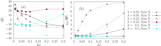
Figure 14: Energy $\langle\hat{H}\rangle$ and spin susceptibility $\chi_{S}(\bm{M})$ as a function of the Trotter step size at different $\lambda$ and for an asymmetric (Sym N) or symmetric (Sym Y) Trotter decomposition. Here, $t=0.1$, $\omega_{0}=2.0$, $\beta=L=6$.

Appendix B Comparison with other QMC approaches

In this section, we provide a short comparison of our method with other approaches. First, we compared it to an algorithm that does not make use of integrating out the phonons and is based on a discrete Hubbard-Stratonovitch decomposition to decouple the $\lambda\hat{K}_{b}^{2}$ term,

$$e^{\Delta\tau\lambda\hat{K}_{b}^{2}}=\frac{1}{4}\sum_{l}\gamma(l)e^{\sqrt{\Delta\tau\lambda}\eta(l)\hat{K}_{b}}\,.$$ (53)

The partition function can be written as

$$Z=\sum_{\left\{l_{b,\tau}\right\}}\left(\prod_{b,\tau}\frac{\gamma(l_{b,\tau})}{4}\right)\int\prod_{b,\tau}dX_{b,\tau}\det\left[1+B(\beta,0)\right]e^{-\Delta\tau\sum_{b,\tau}\left[\frac{m}{2}\left(\frac{X_{b,\tau+1}-X_{b,\tau}}{\Delta \tau}\right)^{2}+\frac{k}{2}X_{b,\tau}^{2}\right]}$$ (54)

with the matrix

$$B(\tau_{1},\tau_{2})=\prod_{\tau=\tau_{2}+\Delta\tau}^{\tau_{1}}\left(\prod_{b}e^{-\Delta\tau gX_{b,\tau}K_{b}}\right)\left(\prod_{b}e^{\sqrt{\Delta\tau\lambda}\eta(l_{b,\tau})K_{b}}\right)e^{\Delta\tau t\sum_{b}K_{b}}\,.$$ (55)

In this case, the stochastic sampling is over the discrete Hubbard-Stratonovitch fields $\{\eta(l_{b,\tau})\}$ and the phonon fields $\{X_{b,\tau}\}$. We used single-spin-flip updates with a Metropolis-Hastings acceptance-rejection step for both kinds of fields.

Motivated by Ref. [4], we also used a Langevin-based algorithm for comparison. In order to employ the Langevin updating scheme, we decoupled the electron interaction with a continuous Hubbard-Stratonovitch transformation,

$$e^{\Delta\tau\lambda\hat{K}_{b}^{2}}=\frac{1}{\sqrt{2\pi}}\int d\phi e^{-\frac{1}{2}\phi^{2}-\sqrt{2\Delta\tau\lambda}\phi\hat{K}_{b}}\,.$$ (56)

In this case, the partition function is given by

$$Z\propto\int\left(\prod_{b,\tau}d\phi_{b,\tau}dX_{b,\tau}\right)\det\left[1+B(\beta,0)\right]e^{-\Delta\tau\sum_{b,\tau}\left[\frac{m}{2}\left(\frac{X_{b,\tau+1}-X_{b,\tau}}{\Delta \tau}\right)^{2}+\frac{k}{2}X_{b,\tau}^{2}\right]}$$ (57)

with

$$B(\tau_{1},\tau_{2})=\prod_{\tau=\tau_{2}+\Delta\tau}^{\tau_{1}}\left(\prod_{b}e^{-\Delta\tau gX_{b,\tau}K_{b}}\right)\left(\prod_{b}e^{-\sqrt{2\Delta\tau\lambda}\phi_{b,\tau}K_{b}}\right)e^{\Delta\tau t\sum_{b}K_{b}}\,.$$ (58)

For an introduction on the Langevin updating scheme, see Refs. [70, 71, 72] and references therein.

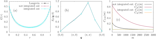
Figure 15: (a) Local imaginary-time Greens function $G(\tau)$ and (b) spin correlation function $S_{S}(\bm{q},0)$ in the first Brillouin zone for $L=4$, $\beta=1.0$, $t=1.0$, $\omega_{0}=3.0$, and $\Delta\tau=0.02$. (c) Correlation functions $C_{S}(m)$ and $C_{K}(m)$ as a function of the number of sweeps $m$ for the same parameters but with simulations performed on a single core. “Integrated out” means we used the algorithm based on the partition function of Eq. (III), “not integrated out” refers to simulations based on Eq. (54), and “Langevin” to the use of Eq. (57).

In Figs. 15(a)-(b), we compare the local imaginary-time Greens function $G(\tau)$ and the spin correlation function $S_{S}(\bm{q},0)$ for all three methods. The results are in good agreement. In general, we noticed a reduction of the autocorrelation time of several observables if the phonons are integrated out. In Fig. 15(c), we compare the autocorrelation time of the equal-time spin correlation function $S_{S}(\bm{M},0)$ and the average kinetic energy $\langle\hat{H}_{t}\rangle=-t\sum_{b}\langle\hat{K}_{b}\rangle$ for the methods based on Eq. (III) and Eq. (54), respectively. The correlation function is defined by

$$C_{\hat{O}}(m)=\frac{\sum_{i=1}^{N_{\mathrm{Bin}}-m}(O_{i}-\langle\hat{O}\rangle)(O_{i+m}-\langle\hat{O}\rangle)}{\sum_{i=1}^{N_{\mathrm{Bin}}-m}(O_{i}-\langle\hat{O}\rangle)^{2}}$$ (59)

with

$$\langle\hat{O}\rangle=\frac{1}{N_{\mathrm{Bin}}}\sum_{i=1}^{N_{\mathrm{Bin}}}O_{i}\,,$$ (60)

where $O_{i}$ is the value of the observable in the $i$th bin and $N_{\mathrm{Bin}}$ is the total number of measurements for a single run. The shorter the autocorrelation time, the faster the correlation function drops to zero, indicating uncorrelated measurements after a certain number of sweeps. A sweep is defined here as visiting every auxiliary field twice and proposing an update with a Metropolis-Hastings acceptance-rejection step. For Fig. 15, we collected around six million sweeps on a single core. The correlation functions for the method with the phonons integrated out need on the order of ten sweeps to drop to zero, whereas for the other method on the order of $10^{3}$ sweeps are required. Comparing the autocorrelation time with the Langevin methods is difficult because the notion of an update is different.

The method used in the main text can be successfully used at higher phonon frequencies compared to the Langevin method because of the negative impact of zeros in the determinant on the latter, see also Ref. [4].

Appendix C Measuring phonon observables

Because we integrated out the phonons in the action, we cannot directly access observables that are functions of phonon variables. To circumvent this issue, we introduced a source term in the phonon action,

$$S_{j}=-\int_{0}^{\beta}d\tau\sum_{b}j_{b}(\tau)X_{b}(\tau)=-\sum_{b,\tau}\Delta\tau j_{b,\tau}X_{b,\tau}\,.$$ (61)

This allows us to formulate the expectation value of a phonon displacement operator as the derivative of the action with respect to the variable $j$ [73, 74],

$$\langle\hat{X}_{b_{1},\tau_{1}}\rangle=\frac{1}{\Delta\tau}\frac{\partial\ln Z}{\partial j_{b_{1},\tau_{1}}}\Big{|}_{\{j_{b,\tau}=0\}}=-\frac{1}{2}\sum_{\tau}(A^{-1})_{\tau_{1},\tau}\langle v_{b_{1},\tau}\rangle\,.$$ (62)

A similar relation holds for the expectation value of the product of two phonon fields,

$$\langle\hat{X}_{b_{1},\tau_{1}}\hat{X}_{b_{2},\tau_{2}}\rangle=\frac{1}{\Delta\tau^{2}}\frac{1}{Z}\frac{\partial^{2}Z}{\partial j_{b_{1},\tau_{1}}\partial j_{b_{2},\tau_{2}}}\Big{|}_{\{j_{b,\tau}=0\}}=\frac{1}{2}\delta_{b_{1},b_{2}}(A^{-1})_{\tau_{1},\tau_{2}}+\frac{1}{4}\sum_{\tau,\tau^{\prime}}(A^{-1})_{\tau_{1},\tau}(A^{-1})_{\tau_{2},\tau^{\prime}}\langle v_{b_{1},\tau}v_{b_{2},\tau^{\prime}}\rangle\,.$$ (63)

Appendix D Additional data

We consider a fixed value $t=1.0$ and vary the phonon frequency $\omega_{0}$. According to the Fig. 1, we expect AFM order at large $\omega_{0}$ and a disordered state (the pseudogap phase) at small $\omega_{0}$.

The average flux remains positive for the parameters considered, with a maximum near $\omega_{0}=2.5$ [Fig. 16(a)]. The derivative of the free energy with respect to the phonon frequency decreases smoothly with increasing $\omega_{0}$ [Fig. 16(b)].

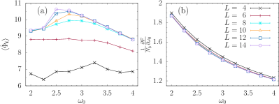
Figure 16: (a) Flux and (b) derivative of the free energy with respect to $\omega_{0}$. Here, $t=1.0$, $\beta=L$.

The correlation ratios of the spin and parity susceptibility at the relevant wave vector ($\bm{M}$ and $\bm{\Gamma}$, respectively) indicate ordering at high phonon frequencies and a phase transition at a critical phonon frequency [Fig. 17].

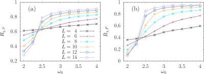
Figure 17: Susceptibility correlation ratio for (a) spin at $\bm{M}$ and (b) parity at $\bm{\Gamma}$. Here, $t=1.0$, $\beta=L$.

Figure 18 shows the equal-time dimer correlation function within the first Brillouin zone at different values of $\omega_{0}$ as well as the single-particle spectral function $A(\bm{k},\omega)$. The dimer correlation function shows no ordering wave vector in the AFM phase and no order develops upon lowering the phonon frequency. However, with decreasing phonon frequency, $(0,\pi)$ VBS fluctuations grow, thereby signaling enhanced proximity to the $(0,\pi)$ ordered VBS phase. This observation is in agreement with the results of Sec. IV.3. At the same time, the gap in the single-particle spectral function remains open upon crossing the critical phonon frequency. Spectral weight accumulates around the edges of the gap with increasing $\omega_{0}$.

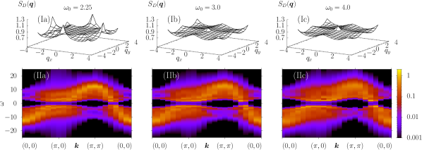
Figure 18: (Ia)-(Ic) Equal-time dimer correlation function in the first Brillouin zone, (IIa)-(IIc) single-particle spectral function $A(\bm{k},\omega)$. Here, $t=1.0$, $\beta=L=14$.