SubT-MRS Dataset: Pushing SLAM Towards All-weather Environments
https://superodometry.com/datasets

Abstract

Simultaneous localization and mapping (SLAM) is a fundamental task for numerous applications such as autonomous navigation and exploration. Despite many SLAM datasets have been released, current SLAM solutions still struggle to have sustained and resilient performance. One major issue is the absence of high-quality datasets including diverse all-weather conditions and a reliable metric for assessing robustness. This limitation significantly restricts the scalability and generalizability of SLAM technologies, impacting their development, validation, and deployment. To address this problem, we present SubT-MRS, an extremely challenging real-world dataset designed to push SLAM towards all-weather environments to pursue the most robust SLAM performance. It contains multi-degraded environments including over 30 diverse scenes such as structureless corridors, varying lighting conditions, and perceptual obscurants like smoke and dust; multimodal sensors such as LiDAR, fisheye camera, IMU, and thermal camera; and multiple locomotions like aerial, legged, and wheeled robots. We develop accuracy and robustness evaluation tracks for SLAM and introduced novel robustness metrics. Comprehensive studies are performed, revealing new observations, challenges, and opportunities for future research.

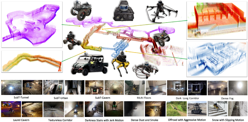
Figure 1: Dense reconstruction from the SubT-MRS dataset, achieved through collaboration with diverse robots equipped with multimodal sensors. Colors represent different challenging environments (tunnels, caves, urban, confined spaces) captured by various robot types (aerial, legged, wheeled). The bottom section showcases a gallery with diverse visual, LiDAR, and mixed degradations.

1 Introduction

Simultaneous Localization and Mapping (SLAM) is essential in robotics since it provides foundational perception and spatial awareness, and enables machines to understand and interact with the physical world in real-time. Therefore, it has a wide range of applications such as autonomous driving and space exploration. Despite significant advancements in both geometric [34, 40, 5] and data-driven SLAM methods [42, 47], existing solutions remain fragile in challenging conditions. One main reason is that existing SLAM algorithms are often developed and evaluated with datasets from controlled environments [3, 11, 17, 20, 35, 33, 38, 54]. For example, KITTI [17, 20] dataset is mostly collected in sunny weather and EuROC-MAV dataset [3] is collected in small well-lit rooms. These datasets, unfortunately, fail to capture the challenges in real-world scenarios, hindering the development of robust SLAM solutions.

To bridge this gap and push SLAM towards all-weather environments, we present an extremely challenging dataset, SubT-MRS, including scenarios featuring various sensor degradation, aggressive locomotions, and extreme-weather conditions. The SubT-MRS dataset comprises 3 years of data from the DARPA Subterranean (SubT) Challenge [1] (2019$-$2021) and extends with an additional 2 years of diverse environments (2022$-$2023), containing mixed indoor and outdoor settings, including long corridors, off-road scenario, tunnels, caves, deserts, forests, and bushlands. Cumulatively, this forms a 5-year dataset encompassing over 2000 hours and 300 kilometers of terrain subjected to multimodal sensors including LiDAR, fisheye cameras, depth cameras, thermal cameras, and IMU; heterogeneous platforms including RC cars, legged robots, aerial robots, and wheeled robots; and extreme obscurant conditions such as dense fog, dust, smoke, and heavy snow.

Additionally, we find there is no well-established metric to evaluate the robustness of a SLAM system. Existing evaluation metrics such as absolute trajectory error (ATE) [3] are not representative of the actual performance in robotic applications. We argue that to ensure the safety control of a robot, SLAM system evaluation should not only focus on poses but also its velocity. Taking robot localization as an example, while a momentary pose error spike may only slightly undermine the overall ATE, however, it can lead to a catastrophic crash in an aerial robotic platform. To effectively gauge the performance of a SLAM algorithm, we introduce a new robustness metric to evaluate the reliability of the SLAM system, particularly examining smoothness and accuracy of velocity estimation.

Lastly, we perform extensive experiments using proposed degradation datasets to benchmark visual and LiDAR SLAM algorithms. These experiments identify the limitations of the existing SLAM systems and evaluate their robustness across the degradation. Our contributions include:

• All-weather Environments  To push SLAM toward all-weather environments, we introduce SubT-MRS, an extremely challenging dataset. Spanning five years, it comprises over 2000 hours and 300 kilometers of accurately measured trajectories. To the best of our knowledge, SubT-MRS is the first real-world dataset that specifically addresses failure scenarios of SLAM by incorporating a variety of degraded conditions, multiple robotic platforms, and diverse sets of multimodal sensors.

• Robustness Metric  To evaluate the actual performance running on robots, we propose a robustness metric, which, to the best of our knowledge, is the first metric evaluating the reliability, safety, and resilience of SLAM.

• SLAM Challenge  We provide a comprehensive benchmark based on the SubT-MRS dataset by conducting ICCV’23 SLAM Challenge. Our evaluation reveals the limitations of state-of-the-art visual and LiDAR SLAM solutions. Furthermore, we conduct extensive experiments to verify robustness metric against various sensor degradation and length of trajectories.

Dataset

Multi-Spectrum

Multi-Degradation

Multi-Robot

Camera

IMU

LiDAR

Thermal

Illumination

Snow

Structureless

SubT

Offroad

Vehicle

Drone

Legged

Handheld

Smoke

EuRoC MAV [3]

✓

✓

✗

✓

✓

✗

✗

✗

✗

✗

✓

✗

✗

PennCOSYVIO [33]

✓

✓

✗

✗

✗

✗

✗

✗

✗

✗

✗

✗

✓

TUM VIO [38]

✓

✓

✗

✗

✗

✗

✗

✗

✗

✗

✗

✗

✓

UZH-FPV [11]

✓

✓

✗

✗

✗

✗

✗

✗

✓

✗

✓

✗

✗

KITTI [18]

✓

✓

✓

✗

✗

✗

✗

✗

✗

✓

✗

✗

✗

Virtual KITTI [15]

✓

✓

✗

✓

✗

✓

✗

✗

✗

✓

✗

✗

✗

College Dataset [51]

✓

✓

✓

✗

✗

✗

✗

✗

✗

✗

✗

✗

✓

RobotCar [28]

✓

✓

✓

✗

✓

✗

✓

✗

✗

✓

✗

✗

✗

UMA VI [54]

✓

✓

✗

✗

✓

✗

✓

✗

✗

✗

✗

✗

✓

UMich [6]

✓

✓

✓

✗

✓

✗

✗

✗

✗

✓

✗

✗

✓

Hilti SLAM [20]

✓

✓

✓

✗

✓

✗

✓

✗

✗

✗

✓

✗

✓

TartanAir [46]

✓

✓

✓

✗

✓

✓

✓

✗

✓

✗

✗

✗

✗

SubT-MRS (Ours)

✓

✓

✓

✓

✓

✓

✓

✓

✓

✓

✓

✓

✓

Table 1: Comparison of SLAM datasets on multi-sensors, multi robots, and multi degradation.

2 Related Work

Multimodal Sensors

Multimodal sensor datasets are crucial for the development of robust SLAM systems, as single sensor modalities are not comprehensive for all scenarios. Existing datasets typically focus on a limited range of modalities, such as monocular or stereo cameras [3, 48], LiDAR [18], event cameras [29], and depth cameras [41]. The KITTI dataset [18], although covering most modalities, is geared towards on-road scenarios and lacks thermal cameras, limiting its applicability to simple, controlled environments. Conversely, the ViViD++ dataset [23] incorporates thermal images in outdoor settings but is deficient in hardware synchronization, posing challenges for SLAM system development. The Weichen dataset [9] offers thermal images in indoor environments with accurate ground truth poses but is confined to motion capture room settings. In contrast, our SubT-MRS dataset delivers a comprehensive suite of time-synchronized multimodal sensors, including LiDAR, monocular and stereo cameras, thermal cameras, depth cameras, and IMU, along with centimeter-level ground truth, catering to a diverse range of research needs.

Heterogeneous Platforms

Developing a robust SLAM system necessitates versatility in handling different motion patterns and various robotic platforms. However, most existing datasets are tailored for single-robot scenarios. While there are a few multi-robot datasets, they typically involve homogeneous platforms [24, 8, 14, 43], posing challenges in evaluating SLAM performance across varied robotic platforms. The AirMuseum dataset [12] includes drones and ground robots but lacks data from legged robots. As a comparison, SubT-MRS dataset features diverse robotic platforms including legged robots, aerial robots, and wheeled robots, operating in varied environments and sensor setups.

Extreme Environmental Conditions

Developing and testing SLAM systems in extreme environmental conditions is crucial for mitigating potential real-world failures. However, most existing SLAM datasets have been primarily limited to single, controlled environments. The TUM-VI [38] and UMA-VI [54] datasets, being indoor-outdoor visual-inertial datasets, pose challenges due to varying illumination and low-texture environments. The EuRoC MAV [3] and UZH-FPV drone racing [11] datasets, popular in the SLAM community, offer data on aggressive drone movements but usually in consistently lit conditions. The KITTI dataset [18], a staple in autonomous driving research for its outdoor LiDAR-Visual-Inertial data. The Hilti SLAM dataset [20] includes both indoor and outdoor LiDAR-visual-inertial datasets with dynamic lighting and confined spaces. However, both of them focus more on accuracy than on a variety of environmental degradations. TartanAir [46] covers most of the challenging environments but it is a simulation dataset that will pose the sim-to-real gap.

In contrast, the SubT-MRS dataset provides 30 varied scenes, encompassing a wide array of environments. These include SubT tunnels, urban areas, caverns, multi-floor structures, dark corridors, and foggy conditions. It also features textureless surfaces, dusty and smoky environments, off-road areas with aggressive motion, and snowy terrains prone to slippage. We include challenging lighting conditions such as extreme darkness and overexposure, along with geometrically complex scenarios like featureless corridors, staircases, and self-similar cave layouts. Additionally, the dataset incorporates perceptual challenges posed by smoke, fog, dust, and various weather conditions.

3 SubT-MRS Dataset

We next present the SubT-MRS dataset from three aspects including its collecting environments and settings, ground truth collection, and the new robustness metric. A detailed comparison with other datasets is listed in Table 1.

Figure 2: An overview of the sensor pack used in SubT-MRS dataset. It is equipped with a Xavier processing unit with hardware time synchronization for multimodal sensors including LiDAR, fisheye cameras, thermal cameras, depth cameras (option), and an IMU.

3.1 All-weather Environments

As mentioned in Sec. 2, the SubT-MRS dataset distinguishes itself through its multimodal sensor setups, heterogeneous robotic platforms, and extreme environmental conditions. This section emphasizes this comprehensive nature pushing SLAM towards all-weather environments.

3.1.1 Multimodal Sensors

Multimodal sensors provide a wealth of information for SLAM systems operating in all-weather environments. This diversity improves scene understanding and strengthens the system’s perception ability. Therefore, We incorporate diverse sensors to ensure system robustness.

Sensor Pack

We embedded 4 Leopard Imaging RGB fisheye cameras, 1 Velodyne puck, 1 Epson M-G365 IMU, 1 FLIR Boson thermal camera, and NVIDIA Jetson AGX Xavier as a sensor pack shown in Figure 2.

Time Synchronization

To ensure the overall consistency of the fused data, we meticulously synchronize the sensors’ time using the ‘pulse per second (PPS)’ technique. As illustrated in Figure 2, the IMU, LiDAR, and thermal camera are directly synchronized with the CPU clock, while the four RGB camera are synchronized using an FPGA board. Consequently, we can effectively manage the time synchronization gap between each pair of sensors not to exceed 3ms.

Fisheye and Thermal Camera Calibration

Camera calibration plays an essential role in the efficiency of a SLAM system. For calibrating the fisheye cameras, we employed the open-source toolkit Kalibr [36], focusing on the intrinsic and extrinsic parameters. Specifically, we use the radial-tangential distortion model to rectify the omnidirectional fisheye camera model. Calibrating thermal cameras, however, poses unique challenges, especially in gathering high-quality thermal data. To tackle this, we set up a 7$\times$9 chessboard, heated by direct sunlight, to generate high-contrast thermal data, ensuring accuracy in the calibration process.

IMU Calibration and Extrinsic Calibration

For Lidar-IMU extrinsic calibration, we utilize the CAD model to obtain the calibration parameters. In the case of Camera-IMU extrinsic calibration, we employ the Kalibr toolbox [36] to estimate the extrinsic matrix. To estimate the sensors’ bias and the random walk noise of the gyroscope and accelerometer, we collected 1-hour static data from the IMU and calibrated it using an Allan variance-based IMU tool [13, 16].

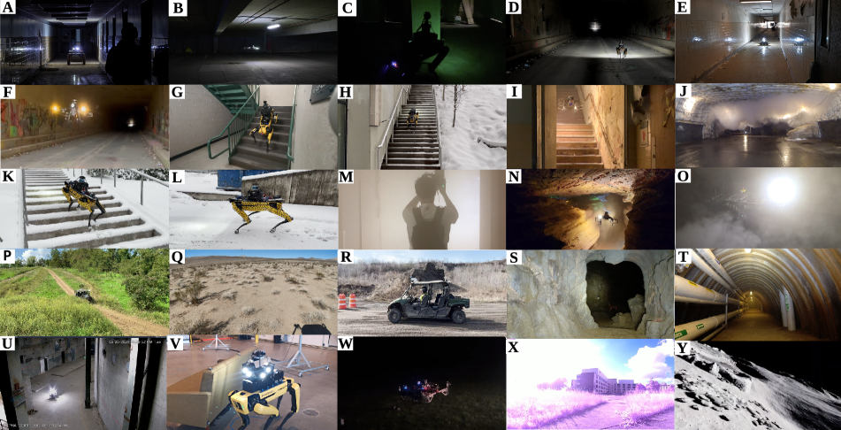
Figure 3: The SubT-MRS datasets were collected across diverse seasons, capturing environments with perceptual challenges such as poor illumination, darkness, and water puddles, where visual sensors falter. They also include geometrically complex areas like long featureless corridors and steep multi-floor structures, challenging LiDAR systems with potential drift. Moreover, these datasets cover conditions with airborne obscurants like dust, fog, snow, and smoke in tough environments, including caves, deserts, long tunnels, and off-road areas.

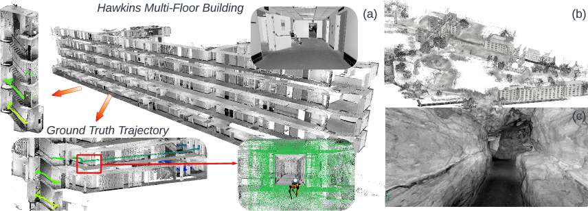
Figure 4: The SubT-MRS dataset facilitates the generation of high-precision ground truth maps and trajectories. Figure (a) shows the ground truth trajectory in multi-floor settings. Figure (b) displays ground truth maps for indoor and outdoor areas, encompassing long corridors, multi-floor structures, and open spaces. Figure (c) features photo-realistic scans based on our ground truth maps in cave environments.

3.1.2 Multi-degraded Environments

SubT-MRS includes multiple challenging environments including visually degraded environments, geometrically degraded environments, and their combination.

Visual Degradation

Poor-quality visual features can significantly hinder the performance of feature extraction processes and disrupt the accuracy of feature matching. Such issues arise in low-light conditions with inconsistent brightness or image noise introduced by air obscurants. SubT-MRS encompasses these challenges and provides a wide range of visual degradation. This includes environments with limited lighting, such as hospital interiors and caves (Figure 3 A-F), as well as smoky or dusty conditions that cause visual obstruction (Figure 3 M-N), and snowy areas with reduced visibility (Figure 3 H, K, and L).

Geometric Degradation

Lack of geometrical features poses significant challenges to LiDAR odometry. The root of this issue often lies in the limited sensing capabilities of LiDAR sensors and the constraints due to their mechanical installation. SubT-MRS captures a variety of environments that exemplify such challenges. It includes long, featureless corridors (Figure 3 E) and staircases (Figure 3 C and G). These scenarios illustrate various forms of geometric degradation, contributing to the improvement of LiDAR odometry systems in challenging conditions.

Mixed Degradation

A mixed visual and geometric degradation can further hinder the performance of SLAM systems. Examples in SubT-MRS include long, dimly lit corridors (Figure 3 A, E, and F), poorly illuminated staircases (Figure 3 C), and environments affected by snowy weather (Figure 3 H, K, and L). In these settings, both LiDAR odometry and visual odometry are prone to failure due to the compounded effects of mixed degradation. The inclusion of such scenarios in SubT-MRS is crucial for evaluating and improving the resilience of multimodal SLAM algorithms.

3.1.3 Heterogeneous Robot Platforms

Most of current datasets focus on single-robot systems, limiting multi-robot SLAM development as shown in Table 1. To address this, we employed diverse robot platforms, including aerial, legged, and wheeled robots, navigating through various environments from urban campuses to medical facilities and natural terrains like caves. This diversity offers a range of scenarios to enhance SLAM algorithms for effective operation in challenging conditions.

Extrinsic Calibration for Multiple Robots

To ensure the multi-robot system shares a common coordinate system, we perform the extrinsic calibration process [37]. It has 2 steps: First, each robot runs Super Odometry [53] to generate its local map using LiDAR data and share it with other robots through a wireless network; Second, the remaining robots identify overlapping regions between their local maps and estimate the extrinsic parameters using GICP [39].

Table 2: SLAM Challenge Results (Blue shadings indicate rankings)

#

Team

Method

Odometry

Device

RealTime (s)

CPU/GPU (%)

RAM (GB)

ATE$\downarrow$

$R_{v}\uparrow$/$R_{w}\uparrow$

Sensors

Type

L

I

C

1

Liu et al

FAST-LIO2 [50], HBA [27]

Filter

Intel i7-9700K

51.310

98.667 / 0

4.052

0.588

0.517/0.770

$\checkmark$

$\checkmark$

2

Yibin et al

LIO-EKF [44]

Filter

Intel i7-10700

0.006

52.167 / 0

0.072

4.313

0.441/0.574

$\checkmark$

$\checkmark$

3

Weitong et al

FAST-LIO[2], Pose Graph[10]

Filter

Intel Xeon(R)E3-1240v5

0.125

22.63 / 0

4.305

0.663

0.473/0.747

$\checkmark$

$\checkmark$

4

Kim et al

FAST-LIO2[49], Point-LIO[19], Quatro[25]

Filter

Intel i5-12500

0.268

101.108 / 0

55.64

3.825

0.479/0.615

$\checkmark$

$\checkmark$

5

Zhong et al

DLO[7], Scan-Context++[21]

SW Opt

AMD Ryzen 9 5900x

0.027

13.289 / 0

1.174

1.209

0.276/0.486

$\checkmark$

$\checkmark$

1

Peng et al

DVI-SLAM [32]

Learning

Intel i9-12900

183.233

- / 149

11 (4)

0.547

0.473/0.788

$\checkmark$

$\checkmark$

2

Jiang et al

LET-NET[26], VINS-Mono[34]

Hybrid

Intel i5-9400

0.064

40.35 / 0

4.337

1.093

0.078/0.322

$\checkmark$

$\checkmark$

3

Thien et al

VR-SLAM[31]

SW Opt

Intel i9-12900

0.142

176.44 / 0

9.111

3.037

0.083/0.372

$\checkmark$

$\checkmark$

4

Li et al

ORB-SLAM3[4]

SW Opt.

Intel i7-10700

0.019

65.028 / 0

0.386

8.975

0.163/0.474

$\checkmark$

$\checkmark$

Table 3: Accuracy Performance on Geometric Degradation. Red numbers represent ATE ranking. * denotes incomplete submissions.

Team	Geometric Degradation (Real World)						Simulation			Mix Degradation			Average
	Urban	Tunnel	Cave	Nuclear_1	Nuclear_2	Laurel_Caverns	Factory	Ocean	Sewerage	Long Corridor	Multi Floor	Block Lidar
Liu et al1	0.307	0.095	0.629	0.122	0.235	0.260	0.889	0.757	0.978	1.454	0.401	0.934	0.588
Weitong et al2	0.26	0.096	0.617	0.120	0.222	0.402	0.998	0.770	1.586	1.254	0.577	1.056	0.663
Kim et al3	0.331	0.092	0.787	0.123	0.270	0.279	10.628	22.425	7.147	2.100	0.650	1.068	3.825
Yibin et al4	1.060	0.220	0.750	0.470	0.620	9.140	4.920	0.280	24.460	2.990	5.500	1.340	4.312
Zhong et al5	1.205	0.695	-	1.175	1.72	2.08	0.889	0.778	1.13	-	-	-	1.209*
Average	0.633	0.240	0.696	0.402	0.6134	2.432	3.665	5.002	7.060	1.950	1.782	1.099

Table 4: Accuracy Performance on Visual Degradation. Red numbers represent ATE ranking. * denotes incomplete submissions.

	Visual Degradation (Real World)						Simulation
Team	Lowlight 1	Lowlight 2	Over Exposure	Flash Light	Smoke Room	Outdoor Night	End of World	Moon	Western Desert	Average
Peng et al1	1.063	1.637	0.503	0.44	0.153	0.827	0.038	0.195	0.070	0.547
Thien et al2	1.081	2.054	1.733	1.054	10.532	7.692	0.753	1.228	1.209	3.037
Jiang et al3	1.019	1.126	1.911	2.341	3.757	11.821	2.154	0.604	4.010	3.193
Li et al4	5.768	7.834	1.757	1.295	5.370	10.766	-	30.07	-	8.98*
Average	2.232	3.163	1.476	1.282	4.953	7.776	0.982	8.024	1.763

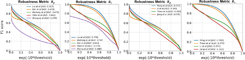
Figure 5: From left to right, it shows robustness metric $R_{p}$ and $R_{r}$ for LiDAR and visual sequences respectively. Note: This is a summary of results for all sequences, with weights based on the trajectory length. The area under the curve (AUC) represents the robustness ($R_{p},R_{r}$). The x-axis shows velocity thresholds for classifying estimated velocities as inliers and the y-axis is F-1 score.

3.2 Ground Truth

Ground Truth Map

As depicted in Figure 4, we utilized the high-precision FARO Focus 3D S120 3D scanner for creating ground-truth maps. This cutting-edge 3D scanner can measure distances up to 120m, with a maximum measurement rate of 976K points per second. The accuracy of the ground truth map is noteworthy, maintaining a range error within $\pm 2$mm. We have developed ground truth models for diverse environments, including subterranean areas like urban areas (350m$\times$350m), caves (150m$\times$200m), and tunnels (100$\times$200m), as well as indoor-outdoor spaces (200m$\times$200m) within the CMU campus. To reduce drift, a loop closure algorithm was applied to correct the poses. Notably, 96% of the scans achieved a position uncertainty of less than 2mm. This ground-truth map is crucial for SLAM development where precision is of utmost importance.

Ground Truth Trajectory

Ground truth trajectories for all sequences are generated based on the ground truth map. In this process, we establish point-to-point, point-to-plane, and point-to-line correspondences[39] between the Ground Truth map and the current LiDAR scan. Our estimated ground truth trajectory is a comprehensive fusion of various constraints derived from the ground truth map, visual odometry, LiDAR odometry, and IMU measurements. This approach ensures the robustness of our solution across diverse environmental conditions. To validate the accuracy of the ground-truth trajectory, we project each LiDAR scan into the world frame and subsequently construct a LiDAR map. It’s worth noting that the trajectories with the highest uncertainty displayed position errors typically falling within the range of $\pm$10cm. See details in our supplementary.

3.3 Robustness Metric

As dicussed in Sec. 1, existing evaluation metrics such as absolute trajectory error (ATE) [3] have limitations in evaluating the SLAM’s robustness in real-world applications. ATE primarily focuses on overall trajectory error and can not effectively capture local errors that have a direct impact on the robot’s safety. For example, a pose spike error might not be immediately noticeable in ATE evaluation, it may result in a crash in an aerial robot control. To address these gaps, we introduce a new robustness metric based on estimated velocity. That is because velocity estimation from SLAM is crucial for the robot’s control system, and significant fluctuations in velocity can directly impact stability, affecting the robot’s safety. The new robustness metric is the area under the curve (AUC) of the F-1 score:

$$F_{1}(e)=\frac{2P(e<{T})R(e<{T})}{P(e<{T})+R(e<{T})},$$ (1)

where the precision $P$ quantifies the precision of the estimated velocity as a percentage: how closely the estimated velocity points lie to the ground truth point and the recall rate $R$ quantifies the estimated velocity’s completeness: to what extent all the ground-truth points are covered. Specifically, an estimated error $e$ is regarded as an inlier, if it is smaller than a threshold ${T}$. To scale the threshold ${T}$ within the range of $[0,1]$, we apply exponential mapping $\exp(-10T)$ when calculating the AUC of F-1 curve.

Position Robustness $R_{p}$ & Rotation Robustness $R_{r}$

The AUC of F-1 score can be defined using both linear velocity and angular velocity, which can reflect the robustness of position and rotation estimation, respectively. Specifically, we define $R_{p}=\rm{AUC}(F_{1}(v_{e}))$ and $R_{r}=\rm{AUC}(F_{1}(\omega_{e}))$, where $v_{e}$ and $\omega_{e}$ are the estimated error of linear velocity and rotation velocity, respectively. Note that not all SLAM solutions can output the velocity at the desired frequency. To address this, we use B-splines [30, 45] to obtain smooth trajectories, compute derivatives for smooth trajectories, and derive estimated linear velocity and angular velocity. For more details, please refer to the supplementary.

4 Experiments

In this section, we will present our works from two perspectives: accuracy evaluation and robustness evaluation.

4.1 Accuracy Evaluation

The results of the open SLAM challenge underscore the necessity for advancements in system robustness. From 29 submissions, we identified 5 winners in the LiDAR category and 4 in the visual category. However, in the sensor fusion track, which addresses both visual and geometric degradation, no submissions met the criteria for success. This result reveals the existing SLAM systems still have lots of space to improve. Sequence characteristics will be detailed in the supplementary material. Table 2 shows the results for both the LiDAR and visual tracks. Unfortunately, there are no current solutions that can balance high accuracy and real-time performance in challenging environments. Since several environments lack geometric features or visual features, the algorithms required more processing times to achieve reasonably high accuracy. Liu et al. at the University of Hong Kong, who achieved the highest accuracy, recorded an Absolute Trajectory Error (ATE) of 0.588m, but each iteration took 51.3 seconds. In the visual track, Peng et al. from the Samsung Research Center attained a leading ATE of 0.547m, but each iteration required 183 seconds.

Table 5: Robustness Performance on Geometric Degradation. Red numbers are robustness ranking. Larger values indicate better robustness.

		Geometric Degradation (Real World)						Simulation			Mix Degradation
Team		Urban	Tunnel	Cave	Nuclear_1	Nuclear_2	Laurel_Caverns	Factory	Ocean	Sewerage	Long Corridor	Multi Floor	Block Lidar	Average
Liu et al1	$R_{p}\uparrow$	0.811	0.865	0.736	0.747	0.504	0.816	0.157	0.135	0.135	0.396	0.529	0.371	0.516
Weitong et al2		0.773	0.838	0.690	0.871	0.739	0.152	0.153	0.149	0.081	0.407	0.456	0.345	0.471
Kim et al4		0.747	0.865	0.737	0.870	0.689	0.777	0.014	0.001	0.010	0.410	0.285	0.345	0.479
Yibin et al3		0.650	0.783	0.557	0.721	0.490	0.481	0.219	0.560	0.019	0.175	0.260	0.370	0.440
Zhong et al5		0.567	0.683	0.204	0.680	0.426	0.447	0.103	0.084	0.122	0	0	0	0.276
Liu et al1	$R_{r}\uparrow$	0.888	0.893	0.816	0.857	0.778	0.861	0.692	0.719	0.652	0.753	0.689	0.643	0.770
Weitong et al2		0.886	0.892	0.811	0.893	0.840	0.598	0.688	0.720	0.514	0.766	0.706	0.644	0.746
Kim et al4		0.680	0.893	0.816	0.893	0.803	0.808	0.198	0.125	0.300	0.802	0.422	0.642	0.615
Yibin et al3		0.624	0.707	0.462	0.733	0.540	0.467	0.862	0.962	0.496	0.477	0.342	0.213	0.573
Zhong et al5		0.731	0.745	0.437	0.757	0.603	0.523	0.688	0.704	0.643	0	0	0	0.485
Average $R_{p}$		0.710	0.807	0.585	0.778	0.570	0.535	0.130	0.186	0.073	0.278	0.306	0.286
Average $R_{r}$		0.762	0.826	0.668	0.827	0.713	0.651	0.626	0.646	0.521	0.560	0.432	0.428

Table 6: Robustness Performance on Visual Degradation. Red numbers are robustness ranking. Larger values indicate better robustness.

		Visual Degradation (Real World)						Simulation
Team		Lowlight 1	Lowlight 2	Over Exposure	Flash Light	Smoke Room	Outdoor Night	End of World	Moon	Western Desert	Average
Peng et al1	$R_{p}\uparrow$	0.357	0.227	0.264	0.203	0.536	0.270	0.699	0.893	0.806	0.472
Thien et al3		0.045	0.070	0.240	0.156	0.131	0.075	0	0.031	0	0.083
Jiang et al 4		0.046	0.039	0.194	0.088	0.242	0.095	0	0	0	0.078
Li et al2		0.342	0.187	0.257	0.208	0.322	0.142	0	0.006	0	0.162
Peng et al1	$R_{r}\uparrow$	0.641	0.581	0.744	0.650	0.878	0.670	0.975	0.975	0.974	0.787
Thien et al3		0.413	0.445	0.610	0.269	0.474	0.487	0.177	0.315	0	0.354
Jiang et al4		0.453	0.452	0.619	0.252	0.542	0.577	0.002	0	0.157	0.339
Li et al2		0.642	0.574	0.657	0.651	0.773	0.660	0.0	0.305	0	0.473
Average $R_{p}$		0.198	0.131	0.239	0.164	0.308	0.146	0.175	0.232	0.202
Average $R_{r}$		0.537	0.513	0.658	0.456	0.667	0.598	0.288	0.399	0.283

LiDAR Track Discussion

To enhance robustness in all-weather environments, a pivotal question arises: what are the limits of current LiDAR SLAM algorithms? Table 3 presents a summary of the ATE/RPE errors observed in real-world geometrically degraded, simulated, and mixed degradation scenarios across the top five teams. In real-world geometrically degraded environments, we observed the first limitation: existing LiDAR solutions struggle in confined spaces such as caves. Almost all algorithms perform worse in Cave (Figure 3S) and Laureal_Cavern environments (Figure 3N) with average ATE 0.696 and 2.432 meters respectively. One reason is that cave environments is the most confined space which may lack sufficient geometric features, compared with other environments like tunnel (Figure 3J) and Urban (Figure 3B) and Nuclear scenes (Figure 3U).

In simulated environments, we encountered the second limitation: existing methods are tailored for fixed motion patterns like vehicles and struggle with unpredictable motion patterns. Since our simulation sequence is derived from TartanAir [46], featuring aggressive and random motion patterns, it might not follow the usual velocity distribution domain and has not been thoroughly tested. As shown in Table 3 (simulation), it resulted in significantly higher ATE errors (5.239m) compared to real-world’s (0.836m).

In mixed degradation environments, the third limitation we found is that existing methods cannot actively select the most informative measurements to adapt to new environments. For example, in the Long Corridor sequence (Figure 3 A) with low lighting and a featureless environment, the scenario is intricately designed for collaborative usage of LiDAR and Visual sensors. Algorithms are expected to utilize visual information in geometrically degraded environments while disregarding it in darkness. Similarly, the Block LiDAR sequences (Figure 3 V) aim to simulate sensor drop scenarios frequently encountered in robotic applications. These sequences involve alternating periods of LiDAR and Visual data loss, challenging algorithms to promptly detect sensor failures and switch to the other modality for SLAM. However, the average ATE error (1.61m) in Table 3 (mixed degradation) is much higher than in geometric degradation scenarios (0.836m), suggesting the above limitations. Details are in the supplementary.

Visual Track Discussion

To improve the robustness, a pivotal question arises: what are the limits of current visual SLAM? To what extent does image quality impact a visual SLAM system? Table 4 shows a summary of ATE errors from real-world and simulation scenarios from the awarded 4 teams. In real-world scenarios, the first limitation is the lack of anti-noise capability in current methods, especially in low-quality image settings. We assessed visual odometry accuracy in visually degraded environments, including low lighting, sunlight overexposure, flashing lights, smoke-filled rooms, and nighttime outdoor settings (Figure 3). Trajectories in conditions like the Smoke Room and Outdoor Night exhibit significantly higher average ATE errors (4.95m, 7.76m respectively). Smoke and night scenes challenge feature extraction and tracking and introduce sensor noise, emphasizing the need for robust anti-noise algorithms. The second limitation is that existing methods struggle to overcome aggressive motion. Even in simulations with relatively good image quality, most methods still show significant average ATE errors (8.024m) on the Moon sequence (Figure 3 Y). See more details in supplementary.

4.2 Robustness Evaluation

The F-1 robustness curve provides a detailed evaluation under different error tolerances, while $R_{p}$ and $R_{r}$ provide an overall measure of robustness that is not dependent on a specific decision threshold. This suggests the flexibility of our new robustness metric. Figure 5 clearly shows the robustness performance of all teams regarding position and rotation, highlighting the differences in robustness between the methods. The values of $R_{p}$ and $R_{r}$, which are the AUC under F-1 curves, are displayed in the brackets of the legends. It reveals that Liu et al. and Peng et al. are the most robust solutions for LiDAR and visual tracks, respectively.

Is the robustness metric robust?

We did extensive experiments on our robustness metric against diverse sensor degradation settings. Table 5 and 6 present a summary of robustness performance in real-world, simulated, and mixed degradation scenarios for both LiDAR and visual sequences. In Table 5, we observe that the average values of $R_{p}$ and $R_{r}$ for the mixed degradation environment (0.290, 0.473) are significantly lower than geometric degradation environments (0.664, 0.754). This observation suggests that the majority of SLAM algorithms exhibit reduced robustness in mixed degradation environments as compared to geometrically degraded ones. This aligns with our expectations and verifies the effectiveness of the robustness metric.

Our robustness ranking, indicated by small red numbers, differs from those on ATE ranking shown in Table 3 and 4. This is because our F-1 score-based metrics $R_{p}$ and $R_{r}$ jointly consider precision and recall rate to provide a balanced evaluation of SLAM performance, considering both metrics across the full spectrum of thresholds. In contrast, the ATE focuses solely on precision, neglecting the trajectory’s completeness (recall). We also evaluate our metric on various synthetic trajectories in the supplementary.

5 Conclusion

We introduce SubT-MRS, a comprehensive SLAM dataset with various sensor data, locomotion patterns, and over 30 degradation types in simulation and real-world settings to push SLAM towards all-weather environments. Additionally, we introduce a new robustness metric to evaluate the reliability of SLAM systems, enhancing robot safety control. 29 teams have tested SubT-MRS in the organized SLAM challenge and we expect that it will serve as a critical benchmark for future SLAM development.

Supplementary Material

Appendix A Overview

We will provide materials from three perspectives: description and analysis of the SubT-MRS dataset, derivation of robustness metric, and more experiment results.

Appendix B SubT-MRS Dataset

In this section, we will provide a more detailed description of our dataset, present key statistics to highlight the challenges inherent in datasets and exhibit a gallery of ground truth 3D models from a range of diverse environments.

B.1 Dataset Description

Table 7: Detailed Dataset Information on LiDAR Track (Blue shadings indicate ATE rankings)

		Degradation Type							Motion Type			Sensor Used
Dataset Seq		Low Light	Textureless	Structureless	Stairs	Smoke/Snow	Aggressive Motion	Repetitive Features	Vehicle Type	Max Speed	Length (m)	Fisheye	LiDAR	Thermal	IMU	Average ATE
Urban	Real World	✓	✓	✗	✗	✓	✗	✗	UGV1	2 m/s	441.86	✗	✓	✗	✓	0.633
Tunnel		✓	✓	✓	✗	✓	✗	✗	UGV2	2 m/s	493.67	✗	✓	✗	✓	0.240
Cave		✓	✓	✓	✗	✗	✗	✓	UGV3	2 m/s	593.79	✗	✓	✗	✓	0.696
Nuclear_1		✓	✓	✗	✗	✓	✗	✗	UGV1	2 m/s	124.92	✗	✓	✗	✓	0.402
Nuclear_2		✓	✓	✗	✗	✓	✗	✗	UGV2	2m/s	1377.37	✗	✓	✗	✓	0.613
Laurel_Cavern		✓	✓	✓	✗	✗	✗	✓	Handheld	2 m/s	490.46	✓	✓	✓	✓	2.432
Factory	Sim	✓	✓	✓	✗	✓	✓	✗	Drone	360 degree/s	160.7	✗	✓	✗	✓	3.665
Ocean		✓	✓	✓	✗	✗	✓	✗	Drone	360 degree/s	127.5	✗	✓	✗	✓	5.002
Sewerage		✓	✓	✓	✗	✗	✓	✗	Drone	360 degree/s	131.0	✗	✓	✗	✓	7.060
Long Corridor	Mix	✓	✓	✓	✗	✗	✓	✗	RC Car	4 m/s	616.45	✓	✓	✗	✓	1.950
Multi Floor		✓	✓	✓	✓	✗	✓	✓	Legged Robot	2 m/s	270	✓	✓	✗	✓	1.782
Block LiDAR		✗	✗	✓	✗	✗	✗	✗	Legged Robot	2 m/s	307.55	✓	✓	✗	✓	1.099

Table 8: Detailed Dataset Information on Visual Track (Blue shadings indicate ATE rankings)

Degradation Type

Motion Type

Sensor Used

Dataset Seq

Low Lighting

Textureless

Over Exposure

Darkness

Smoke

Aggressive Motion

Repetitive Features

Vehicle Type

Max Speed

Length (m)

Fisheye

LiDAR

Thermal

IMU

Average ATE

Low Light1

Real World

✓

✓

✓

✗

✗

✗

✓

Handheld

2 m/s

400.61

✓

✗

✓

✓

2.232

Low Light2

✓

✓

✓

✗

✗

✗

✓

Handheld

2 m/s

583.19

✓

✗

✓

✓

0.633

Over Exposure

✗

✗

✓

✗

✗

✗

✗

Legged Robot

2 m/s

456.26

✓

✗

✓

✓

3.163

Flash Light

✓

✓

✓

✗

✗

✗

✗

Legged Robot

2 m/s

147.75

✓

✗

✓

✓

1.476

Smoke Room

✓

✓

✗

✓

✓

✗

✗

RC car

2m/s

104.84

✓

✗

✓

✓

4.953

Outdoor Night

✓

✓

✗

✓

✗

✗

✗

Legged Robot

2 m/s

254.03

✓

✗

✓

✓

7.776

End of World

Sim

✓

✓

✗

✗

✗

✓

✗

Drone

350 degree/s

280

✓

✗

✗

✓

0.982

Moon

✓

✓

✗

✗

✗

✓

✓

Drone

60 degree/s

850

✓

✗

✗

✓

8.024

Western Desert

✓

✓

✗

✓

✗

✓

✓

Drone

80 degree/s

600

✓

✗

✗

✓

1.763

We presented comprehensive details about our datasets, including specific challenges, types of motion, and the sensors used, as shown in Table 7 and 8. The average ATE (Absolute Trajectory Error) is computed based on results of the top 5 teams and blue-shaded area reflects ranking of ATE.

Overview of LiDAR Track in Real-World

Table 7 provide comprehensive dataset information from the LiDAR track, encompassing geometric degradation in real-world and simulated environments, as well as mixed degradation involving both geometric and visual factors. It’s important to note that place recognition in cave settings presents challenges for backend optimization, owing to the similarity and repetitiveness of geometric features. Consequently, this results in an average ATE of 2.432 m, which is the highest.

Overview of LiDAR Track in Simulation

The dataset was collected using a drone. Its primary challenges arose from the drone’s aggressive motion with a maximum angular velocity of 360 degrees per second. Additionally, the Factory sequence, shown in Figure 11 A, was captured in snowy conditions. Such a dynamic environment can impair the performance of SLAM systems by introducing snow noise.

Overview of LiDAR Track in Mixed Degradation

It includes both LiDAR and visual degradation such as Long Corridor and Multi-floor sequence, which will be illustrated in Sec B.2. The Block LiDAR sequence is designed to simulate sensor dropout scenarios, which are frequently encountered in the field of robotics. To evaluate the failure-aware capabilities of the systems, we intentionally disrupted the LiDAR measurements midway through the run. Our objective was to observe whether the algorithm could detect off-normal scenarios and switch to alternate modalities.

Overview of Visual Track

Tables 8 provide comprehensive information from the visual track, including degradation from real-world and simulated environments. In real-world settings, the Low Light 1 and Low Light 2 sequences, captured in cave environments, presented place recognition challenges due to the similarity and repetitiveness of features, as shown in Figure 10 A and B. These environments look alike despite being in different locations. Figure 10 F, G, and D depict lighting changes from the Flash Light and Over Exposure sequence, which breaks the photometric consistency assumption on feature tracking. Figure 10 E depicts scenarios from the Smoke Room sequence, where the dynamic smoke not only reduces the number of detected features but also significantly increases noise in feature matching. Figure 10 H exhibits image noise in the Outdoor Night sequence, and I shows the fisheye camera covered to simulate sensor dropout scenarios. In the simulated environments, the scenes captured are shown in Figure 11 D, E, and F, respectively.

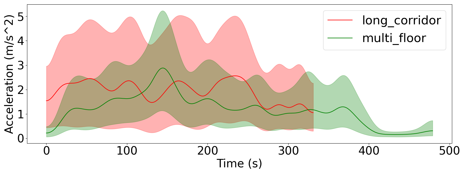
Figure 6: The graphs display average acceleration over time for all runs conducted in the long corridor and multi-floor environments. The shaded area indicates the variance in acceleration.

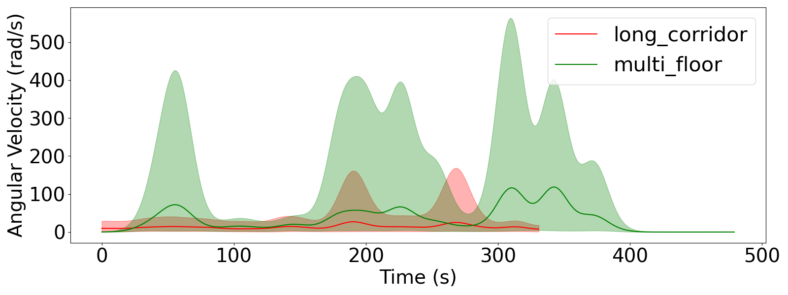
Figure 7: The graphs display average angular velocity over time for all runs conducted in the long corridor and multi-floor environments. The shaded area indicates the variance in angular velocity.

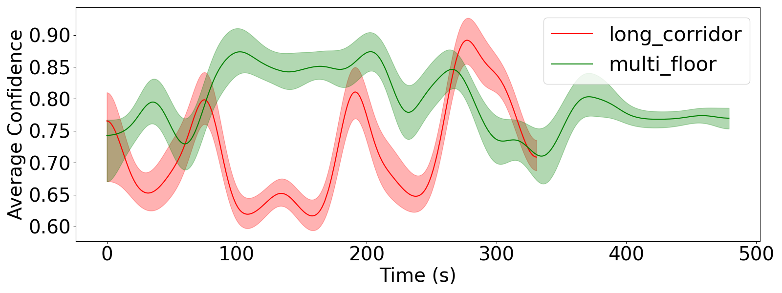
Figure 8: The graphs display the average confidence value of state estimation over time for all runs conducted in the long corridor and multi-floor environments. The shaded area indicates the variance in confidence value.

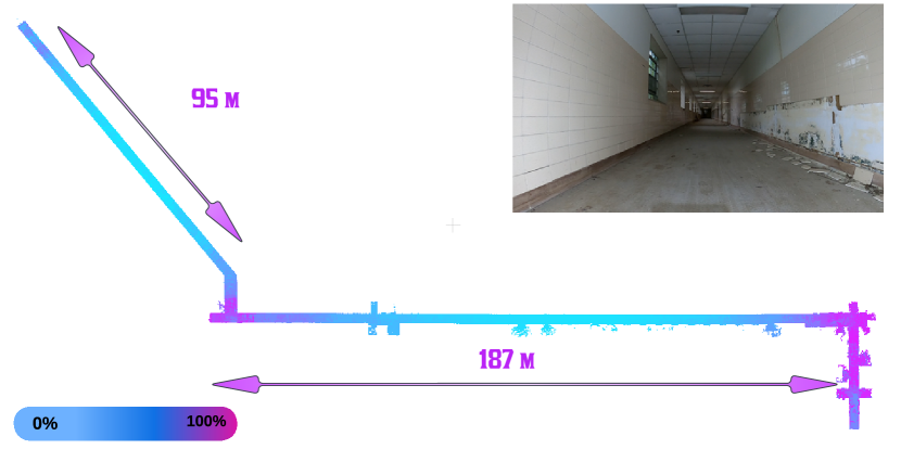
Figure 9: The Confidence Map in Long Corridor Environments. The central region of the long corridor displays the most blue areas, indicating higher uncertainty. This is primarily due to the limited constraints in the forward direction in the corridor, leading to increased mapping uncertainty.

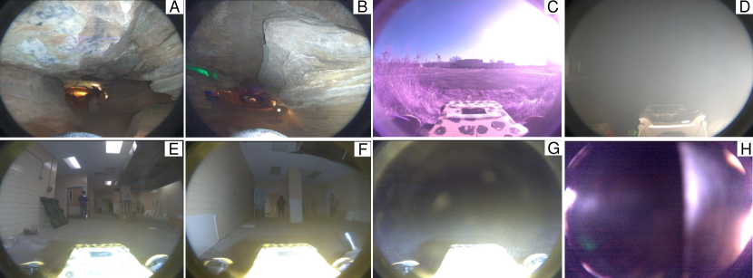
Figure 10: Real-world datasets captured with our fisheye camera to exhibit various visual degradations.

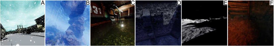
Figure 11: Simulation from both LiDAR/Visual Track. A: Factory B: Ocean C: Swerage D: End of world E: Moon F: Western Desert

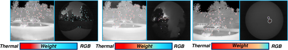
Figure 12: Feature Tracking in Smoke Environments on RGB and Thermal Images: The sequence from left to right on weight illustrates a decrease in feature tracking on RGB images and a corresponding increase on thermal images.

B.2 Dataset Statistics

In this section, we will analyze our dataset from three perspectives: degeneracies in LiDAR track, degeneracies in visual track, and an analysis of robot locomotion.

Degeneracies in LiDAR

To help users understand the challenges of our dataset, we use various metrics to measure the difficulty of dataset statistically. The statistics include acceleration, angular velocity rate, and confidence value. The acceleration and angular velocity are used to measure the motion pattern of this dataset and a confidence value is provided by Super Odometry[53] to evaluate the degradation level of environments. In the LiDAR track, we select 2 typical challenging environments: Long corridor and Multi Floor sequence to evaluate.

Figure 14 and Figure 13 demonstrate that the Long Corridor sequences exhibit greater acceleration compared to the multi-floor sequences, while the Multi-Floor sequences experience more angular velocity changes than those in long corridor environments. Given that Super Odometry can assess the confidence of state estimation, we utilize this metric to gauge the overall challenges of the dataset. It is observed that the long corridor shows lower confidence values most of the time, indicating that it is a more challenging environment for LiDAR SLAM systems. Figure 9 further illustrated the confidence value of map in 3D space.

Degeneracies in Visual

We selected a smoke environment to specifically illustrate degeneracy, showcasing the tracked feature count in both thermal and RGB images, as shown in Figure 12. In this setting, we applied a learning-based feature extraction pipeline[52], to these multispectral images. With increasing smoke density, the thermal images are not influenced, whereas RGB images tend to add noise to the feature tracking process. Therefore, in such scenarios, an optimal SLAM solution should gradually prioritize the thermal camera as primary sensor for state estimation.

Heterogeneous Robot Locomotion

Our dataset, sourced from heterogeneous robots, allows for an analysis of their movement patterns to identify which robots yield the more challenging datasets. Figure 14 and Figure 13 present the average acceleration and angular velocity across all runs from different robots. These figures highlight that the dataset from the canary drone poses greater challenges compared to others, evidenced by its higher frequency of peaks in both acceleration and angular velocity.

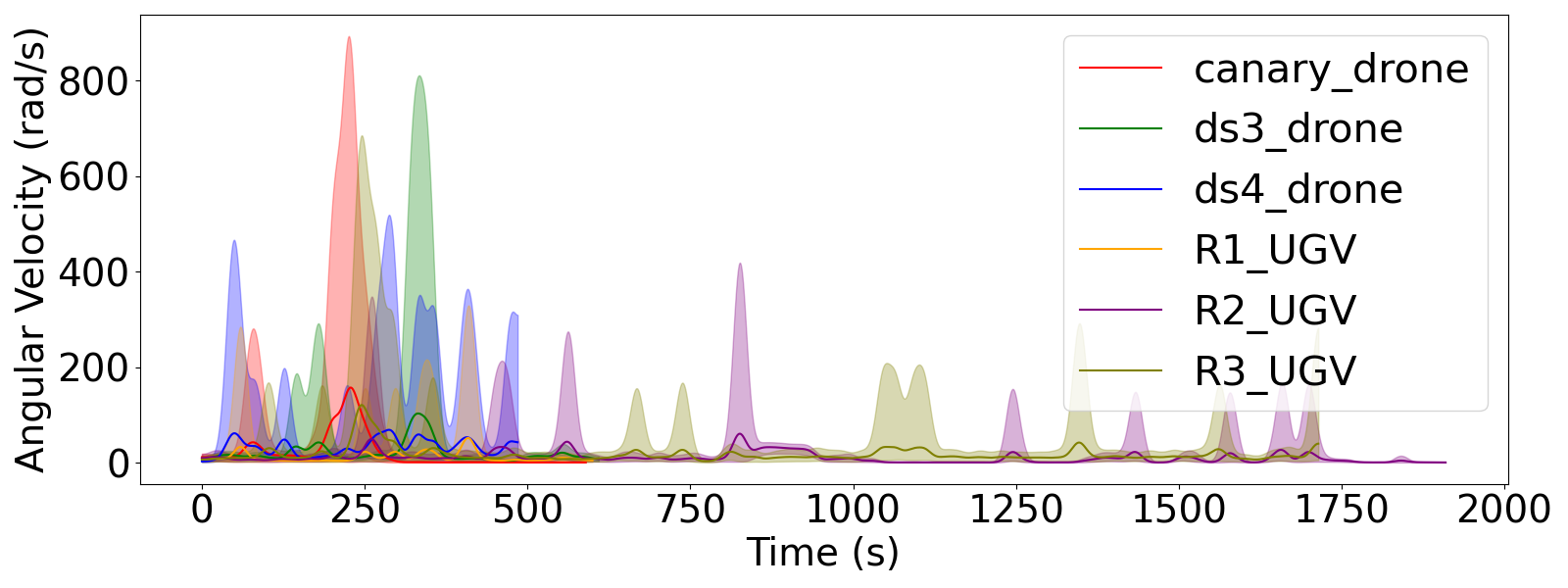
Figure 13: The graph displays the angular velocity over time for all runs conducted in the SubT environment. The shaded area indicates the variance in angular velocity.

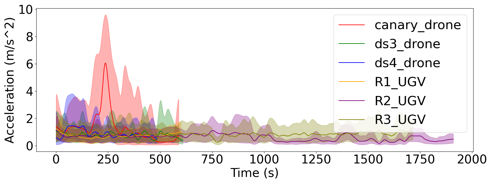
Figure 14: The graph displays the acceleration over time for all runs conducted in the SubT environment. The shaded area indicates the variance in acceleration.

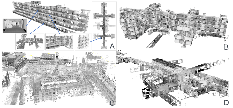
Figure 15: The Ground Truth Model in SubT-MRS Dataset. A: Long Corridor B: MultiFloor C: Campus Outdoor D: Campus Indoor

B.3 Ground Truth Model

In this section, we are pleased to present our extensive collection of Ground Truth 3D Models, as displayed in Figure 15. This collection includes a ground truth model of a university campus, covering both indoor and outdoor areas, extensive loop mapping for long corridor and multi floor environments. Importantly, all ground truth models were captured using a FARO scanner, guaranteeing an accuracy within 10 cm.

Appendix C Derivation of Robustness Metric

As introduced in the main paper Sec 3.3, we describe how to use B-spline to derive estimated linear and angular velocity. Additionally, we will show the steps of robustness metric calculation.

B-splines

We adopt B-splines [30] to interpolate the given trajectory, yielding continuous-time trajectories in $SE(3)$. The continuous trajectory is decided by control poses $T_{w,i}$, where $T_{w,i}$ is the estimated poses at time $t_{i}$ in a world coordinate system $w$. According to the locality of the cubic B-spline basis, the value of the spline curve at any time $t$ is decided by four control poses. We use one absolute pose, $T_{w,i-1}$, and three incremental poses, parametrized by twists $\xi_{i}$. More specifically, the spline trajectory is given by

$$T_{w,s}(u(t))=T_{w,i-1}\prod_{j=1}^{3}\exp(\mathbf{B}_{j}(u(t))\xi_{i+j-1})$$ (2)

where the $\exp$ denotes the matrix exponential. $u(t)=(t-t_{i})/\Delta t\in[0,1]$ and $t_{i}=i\Delta t$ are used in the cumulative basis functions for the B-splines.

$$\bar{\mathbf{B}}(u)=C\begin{bmatrix}1\\ u\\ u^{2}\\ u^{3}\end{bmatrix},\quad C=\begin{bmatrix}6&0&0&0\\ 5&3&-3&1\\ 1&3&3&-2\\ 0&0&0&1\end{bmatrix},$$ (3)

In Eq.2, $\mathbf{B}_{j}$ is the $j$-th entry (0-based) of vector $\mathbf{B}$. The incremental pose from time $t_{i-1}$ to $t_{i}$ is encoded by twist

$$\xi_{i}=\log(T_{w,i-1}^{-1}T_{w,i}),$$ (4)

$$\frac{\partial}{\partial t_{s}}T_{w,s}(u(t))=[\Delta\dot{R},\Delta\dot{T}]=[\mathbf{\omega}_{w},\mathbf{v}_{w}]$$ (5)

We differentiate the spline trajectory as presented in Eq. 5 to obtain estimates of the velocity, denoted as $\mathbf{v}_{w}$, and the angular velocity, denoted as $\mathbf{\omega}_{w}$. We sampled velocities from both the interpolated ground truth trajectory and the trajectory estimated via B-spline, establishing velocity correspondences based on time stamps.

Table 9: Accuracy Performance on LiDAR Degradation. Red numbers represent ATE/RPE ranking. * denotes incomplete submissions.

		Real World						Simulation			Mix Degradation
Team		Urban	Tunnel	Cave	Nuclear_1	Nuclear_2	Laurel_Caverns	Factory	Ocean	Sewerage	Long Corridor	Multi Floor	Block Lidar	Average
Liu et al1	ATE	0.307	0.095	0.629	0.122	0.235	0.260	0.889	0.757	0.978	1.454	0.401	0.934	0.588
Yibin et al4		1.060	0.220	0.750	0.470	0.620	9.140	4.920	0.280	24.460	2.990	5.500	1.340	4.312
Weitong et al2		0.26	0.096	0.617	0.120	0.222	0.402	0.998	0.770	1.586	1.254	0.577	1.056	0.663
Kim et al3		0.331	0.092	0.787	0.123	0.270	0.279	10.628	22.425	7.147	2.100	0.650	1.068	3.825
Zhong et al5		1.205	0.695	-	1.175	1.72	2.08	0.889	0.778	1.13	-	-	-	1.209*
Liu et al1	RPE	0.038	0.032	0.055	0.028	0.048	0.040	0.191	0.174	0.188	0.088	0.059	0.148	0.091
Yibin et al3		0.130	0.090	0.150	0.130	0.200	0.200	0.040	0.040	0.160	0.630	0.280	0.180	0.186
Weitong et al2		0.038	0.032	0.056	0.029	0.049	0.046	0.190	0.183	0.243	0.086	0.054	0.166	0.097
Kim et al4		0.098	0.032	0.055	0.028	0.054	0.046	0.861	0.535	0.401	0.093	0.26	0.167	0.219
Zhong et al5		0.157	0.062	-	0.079	0.1062	0.0937	0.706	0.691	0.617	-	-	-	0.313*

Table 10: Accuracy Performance on Visual Degradation. Red numbers represent ATE/RPE ranking. * denotes incomplete submissions.

		Real World						Simulation
Team		Lowlight 1	Lowlight 2	Over Exposure	Flash Light	Smoke Room	Outdoor Night	End of World	Moon	Western Desert	Average
Peng et al1	ATE	1.063	1.637	0.503	0.44	0.153	0.827	0.038	0.195	0.070	0.547
Jiang et al3		1.019	1.126	1.911	2.341	3.757	11.821	2.154	0.604	4.010	3.193
Thien et al2		1.081	2.054	1.733	1.054	10.532	7.692	0.753	1.228	1.209	3.037
Li et al4		5.768	7.834	1.757	1.295	5.370	10.766	-	30.07	-	8.98*
Peng et al1	RPE	0.058	0.063	0.051	0.149	0.026	0.064	0.002	0.014	0.01	0.048
Jiang et al3		0.190	0.203	0.258	0.307	0.884	3.427	3.982	0.792	7.477	1.947
Thien et al2		0.197	0.186	0.181	0.231	0.071	0.279	0.471	0.007	0.777	0.266
Li et al4		0.088	0.088	0.124	0.160	0.911	0.478	-	0.347	-	0.314*

Robustness Metric Calculation

We introduce the F-score [22] to evaluate the robustness of SLAM algorithms. The robustness metric can be calculated in the following steps:

Algorithm 1 Robustness Metric Calculation

Input: Trajectory $T_{w,i}$, ground truth velocities $\mathbf{v}_{gt}^{w},\boldsymbol{\omega}_{gt}^{w}$

Output: Robustness Metric

Step 1: Smooth trajectory with B-spline on $T_{w,i}$

Step 2: Derive $\mathbf{v}_{est}^{w},\mathbf{\omega}_{est}^{w}$ from smoothed trajectory

Step 3: Calculate distances: $\mathbf{v}_{dis}=||\mathbf{v}_{gt}^{w}-\mathbf{v}_{est}^{w}||$, $\boldsymbol{\omega}_{dis}=||\boldsymbol{\omega}_{gt}^{w}-\boldsymbol{\omega}_{est}^{w}||$

Step 4: Compute F-scores $F(\mathbf{v}_{dis}),F(\boldsymbol{\omega}_{dis})$ for various thresholds

Step 5: Plot F-scores against thresholds; area under curve is robustness metric

Appendix D Experiments

In this section, we provide detailed experiments assessing accuracy and robustness, which were not included in the main paper due to length constraints. It should be noted that the main paper already includes comprehensive experiments on our datasets and presents summarized conclusions. The additional experiments here serve as supplementary evidence supporting the conclusions drawn in Sections 4.1 and 4.2 of our paper.

D.1 Accuracy Evaluation

In section 4.1, we presented Absolute Trajectory Error (ATE) values for the LiDAR and visual tracks. We omitted the RPE results due to the constraints of paper length. Table 9 and Table 10 provide RPE results.

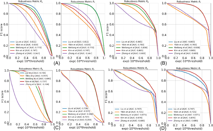
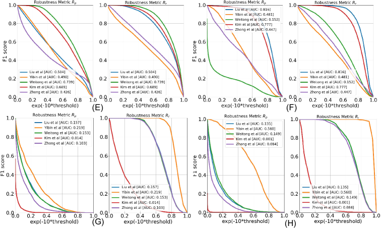
Figure 16: The image, arranged from left to right, displays the robustness metrics $R_{p}$ and $R_{r}$ from LiDAR track teams: (A) Urban, (B) Tunnel, (C) Cave, and (D) Nuclear_1 (E) Nuclear_2 (F) Laurel Cavern (G) Factory (H) Ocean

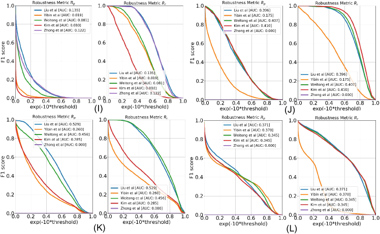
Figure 17: The image, arranged from left to right, displays the robustness metrics $R_{p}$ and $R_{r}$ from LiDAR track teams: (I) Sewerage, (J) Long Corridor, (K) Multi Floor, (L) Block LiDAR

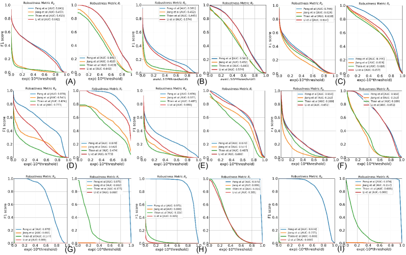
Figure 18: The image, arranged from left to right, displays the robustness metrics $R_{p}$ and $R_{r}$ from visual track teams: (A) Low Light1, (B) Low Light2, (C) Over Exposure, and (D) Flash Light,(E) Smoke Room (F) Outdoor Night, (G) End of World, (H) Moon (I) Western Desert

D.2 Robustness Evaluation

In section 4.2, we presented a summary of the robustness metrics for the LiDAR and visual tracks and omitted the detailed robustness plots for each sequence due to the constraints of the paper’s length. Figure 16 and Figure 17 illustrate the robustness metrics on each sequence for the LiDAR teams, while Figure 18 show the results from visual track teams.

References

- [1] https://www.darpa.mil/program/darpa-subterranean-challenge.
- Bai et al. [2022] Chunge Bai, Tao Xiao, Yajie Chen, Haoqian Wang, Fang Zhang, and Xiang Gao. Faster-lio: Lightweight tightly coupled lidar-inertial odometry using parallel sparse incremental voxels. IEEE Robotics and Automation Letters, 7(2):4861–4868, 2022.
- Burri et al. [2016] Michael Burri, Janosch Nikolic, Pascal Gohl, Thomas Schneider, Joern Rehder, Sammy Omari, Markus W Achtelik, and Roland Siegwart. The EuRoC micro aerial vehicle datasets. The International Journal of Robotics Research, 2016.
- Campos et al. [2021a] Carlos Campos, Richard Elvira, Juan J Gómez Rodríguez, José MM Montiel, and Juan D Tardós. Orb-slam3: An accurate open-source library for visual, visual–inertial, and multimap slam. IEEE Transactions on Robotics, 37(6):1874–1890, 2021a.
- Campos et al. [2021b] Carlos Campos, Richard Elvira, Juan J. Gómez Rodríguez, José M. M. Montiel, and Juan D. Tardós. Orb-slam3: An accurate open-source library for visual, visual–inertial, and multimap slam. IEEE Transactions on Robotics, 37(6):1874–1890, 2021b.
- Carlevaris-Bianco et al. [2016] Nicholas Carlevaris-Bianco, Arash K Ushani, and Ryan M Eustice. University of michigan north campus long-term vision and lidar dataset. The International Journal of Robotics Research, 35(9):1023–1035, 2016.
- Chen et al. [2022a] Kenny Chen, Brett T. Lopez, Ali-akbar Agha-mohammadi, and Ankur Mehta. Direct lidar odometry: Fast localization with dense point clouds. IEEE Robotics and Automation Letters, 7(2):2000–2007, 2022a.
- Chen et al. [2022b] Long Chen, Yuchen Li, Chao Huang, Bai Li, Yang Xing, Daxin Tian, Li Li, Zhongxu Hu, Xiaoxiang Na, Zixuan Li, et al. Milestones in autonomous driving and intelligent vehicles: Survey of surveys. IEEE Transactions on Intelligent Vehicles, 8(2):1046–1056, 2022b.
- Dai et al. [2021] Weichen Dai, Yu Zhang, Shenzhou Chen, Donglei Sun, and Da Kong. A multi-spectral dataset for evaluating motion estimation systems. In 2021 IEEE International Conference on Robotics and Automation (ICRA), pages 5560–5566. IEEE, 2021.
- Dellaert et al. [2017] Frank Dellaert, Michael Kaess, et al. Factor graphs for robot perception. Foundations and Trends® in Robotics, 6(1-2):1–139, 2017.
- Delmerico et al. [2019] Jeffrey Delmerico, Titus Cieslewski, Henri Rebecq, Matthias Faessler, and Davide Scaramuzza. Are we ready for autonomous drone racing? the UZH-FPV drone racing dataset. In IEEE Int. Conf. Robot. Autom. (ICRA), 2019.
- Dubois et al. [2020] Rodolphe Dubois, Alexandre Eudes, and Vincent Frémont. Airmuseum: a heterogeneous multi-robot dataset for stereo-visual and inertial simultaneous localization and mapping. In 2020 IEEE International Conference on Multisensor Fusion and Integration for Intelligent Systems (MFI), pages 166–172, 2020.
- El-Sheimy et al. [2008] Naser El-Sheimy, Haiying Hou, and Xiaoji Niu. Analysis and modeling of inertial sensors using allan variance. IEEE Transactions on Instrumentation and Measurement, 57(1):140–149, 2008.
- Feng et al. [2022] Dapeng Feng, Yuhua Qi, Shipeng Zhong, Zhiqiang Chen, Yudu Jiao, Qiming Chen, Tao Jiang, and Hongbo Chen. S3e: A large-scale multimodal dataset for collaborative slam. arXiv preprint arXiv:2210.13723, 2022.
- Gaidon et al. [2016] Adrien Gaidon, Qiao Wang, Yohann Cabon, and Eleonora Vig. Virtual worlds as proxy for multi-object tracking analysis. In Proceedings of the IEEE conference on computer vision and pattern recognition, pages 4340–4349, 2016.
- Gao [2018] Wenliang Gao. A ros package tool to analyze the imu performance, 2018.
- Geiger et al. [2012] Andreas Geiger, Philip Lenz, and Raquel Urtasun. Are we ready for autonomous driving? The KITTI Vision Benchmark Suite. In Conference on Computer Vision and Pattern Recognition (CVPR), 2012.
- Geiger et al. [2013] Andreas Geiger, Philip Lenz, Christoph Stiller, and Raquel Urtasun. Vision meets robotics: The kitti dataset. The International Journal of Robotics Research, 32(11):1231–1237, 2013.
- He et al. [2023] Dongjiao He, Wei Xu, Nan Chen, Fanze Kong, Chongjian Yuan, and Fu Zhang. Point-lio: Robust high-bandwidth light detection and ranging inertial odometry. Advanced Intelligent Systems, page 2200459, 2023.
- Helmberger et al. [2022] Michael Helmberger, Kristian Morin, Beda Berner, Nitish Kumar, Giovanni Cioffi, and Davide Scaramuzza. The hilti slam challenge dataset. IEEE Robotics and Automation Letters, 7(3):7518–7525, 2022.
- Kim and Kim [2018] Giseop Kim and Ayoung Kim. Scan context: Egocentric spatial descriptor for place recognition within 3d point cloud map. In 2018 IEEE/RSJ International Conference on Intelligent Robots and Systems (IROS), pages 4802–4809. IEEE, 2018.
- Knapitsch et al. [2017] Arno Knapitsch, Jaesik Park, Qian-Yi Zhou, and Vladlen Koltun. Tanks and temples: Benchmarking large-scale scene reconstruction. ACM Transactions on Graphics (ToG), 36(4):1–13, 2017.
- Lee et al. [2022] Alex Junho Lee, Younggun Cho, Young-sik Shin, Ayoung Kim, and Hyun Myung. Vivid++: Vision for visibility dataset. IEEE Robotics and Automation Letters, 7(3):6282–6289, 2022.
- Leung et al. [2011] Keith YK Leung, Yoni Halpern, Timothy D Barfoot, and Hugh HT Liu. The utias multi-robot cooperative localization and mapping dataset. The International Journal of Robotics Research, 30(8):969–974, 2011.
- Lim et al. [2022] Hyungtae Lim, Suyong Yeon, Suyong Ryu, Yonghan Lee, Youngji Kim, Jaeseong Yun, Euigon Jung, Donghwan Lee, and Hyun Myung. A single correspondence is enough: Robust global registration to avoid degeneracy in urban environments. page Accepted. To appear, 2022.
- Lin et al. [2023] Yicheng Lin, Shuo Wang, Yunlong Jiang, and Bin Han. Breaking of brightness consistency in optical flow with a lightweight cnn network, 2023.
- Liu et al. [2023] Zheng Liu, Xiyuan Liu, and Fu Zhang. Efficient and consistent bundle adjustment on lidar point clouds. IEEE Transactions on Robotics, 2023.
- Maddern et al. [2017] Will Maddern, Geoffrey Pascoe, Chris Linegar, and Paul Newman. 1 year, 1000 km: The oxford robotcar dataset. The International Journal of Robotics Research, 36(1):3–15, 2017.
- Mueggler et al. [2017] Elias Mueggler, Henri Rebecq, Guillermo Gallego, Tobi Delbruck, and Davide Scaramuzza. The event-camera dataset and simulator: Event-based data for pose estimation, visual odometry, and slam. The International Journal of Robotics Research, 36(2):142–149, 2017.
- Mueggler et al. [2018] Elias Mueggler, Guillermo Gallego, Henri Rebecq, and Davide Scaramuzza. Continuous-time visual-inertial odometry for event cameras. IEEE Transactions on Robotics, 34(6):1425–1440, 2018.
- Nguyen et al. [2023] Thien Hoang Nguyen, Shenghai Yuan, and Lihua Xie. Vr-slam: A visual-range simultaneous localization and mapping system using monocular camera and ultra-wideband sensors, 2023.
- Peng et al. [2023] Xiongfeng Peng, Zhihua Liu, Weiming Li, Ping Tan, SoonYong Cho, and Qiang Wang. Dvi-slam: A dual visual inertial slam network, 2023.
- Pfrommer et al. [2017] Bernd Pfrommer, Nitin Sanket, Kostas Daniilidis, and Jonas Cleveland. Penncosyvio: A challenging visual inertial odometry benchmark. In 2017 IEEE International Conference on Robotics and Automation (ICRA), pages 3847–3854. IEEE, 2017.
- Qin et al. [2018] Tong Qin, Peiliang Li, and Shaojie Shen. Vins-mono: A robust and versatile monocular visual-inertial state estimator. IEEE Transactions on Robotics, 34(4):1004–1020, 2018.
- Ramezani et al. [2020] Milad Ramezani, Yiduo Wang, Marco Camurri, David Wisth, Matias Mattamala, and Maurice Fallon. The newer college dataset: Handheld lidar, inertial and vision with ground truth. In 2020 IEEE/RSJ International Conference on Intelligent Robots and Systems (IROS), pages 4353–4360. IEEE, 2020.
- Rehder et al. [2016] Joern Rehder, Janosch Nikolic, Thomas Schneider, Timo Hinzmann, and Roland Siegwart. Extending kalibr: Calibrating the extrinsics of multiple imus and of individual axes. In 2016 IEEE International Conference on Robotics and Automation (ICRA), pages 4304–4311. IEEE, 2016.
- Scherer et al. [2022] Sebastian Scherer, Vasu Agrawal, Graeme Best, Chao Cao, Katarina Cujic, R Darnley, R DeBortoli, E Dexheimer, B Drozd, R Garg, et al. Resilient and modular subterranean exploration with a team of roving and flying robots. Field Robotics, 2022.
- Schubert et al. [2018] David Schubert, Thore Goll, Nikolaus Demmel, Vladyslav Usenko, Jörg Stückler, and Daniel Cremers. The tum vi benchmark for evaluating visual-inertial odometry. In 2018 IEEE/RSJ International Conference on Intelligent Robots and Systems (IROS), pages 1680–1687. IEEE, 2018.
- Segal et al. [2009] Aleksandr Segal, Dirk Haehnel, and Sebastian Thrun. Generalized-icp. In Robotics: science and systems, page 435. Seattle, WA, 2009.
- Shan et al. [2020] Tixiao Shan, Brendan Englot, Drew Meyers, Wei Wang, Carlo Ratti, and Rus Daniela. Lio-sam: Tightly-coupled lidar inertial odometry via smoothing and mapping. In IEEE/RSJ International Conference on Intelligent Robots and Systems (IROS), pages 5135–5142. IEEE, 2020.
- Sturm et al. [2012] J. Sturm, N. Engelhard, F. Endres, W. Burgard, and D. Cremers. A benchmark for the evaluation of rgb-d slam systems. In Proc. of the International Conference on Intelligent Robot Systems (IROS), 2012.
- Teed and Deng [2021] Zachary Teed and Jia Deng. Droid-slam: Deep visual slam for monocular, stereo, and rgb-d cameras. Advances in neural information processing systems, 34:16558–16569, 2021.
- Tian et al. [2023] Yulun Tian, Yun Chang, Long Quang, Arthur Schang, Carlos Nieto-Granda, Jonathan P How, and Luca Carlone. Resilient and distributed multi-robot visual slam: Datasets, experiments, and lessons learned. arXiv preprint arXiv:2304.04362, 2023.
- Vizzo et al. [2023] Ignacio Vizzo, Tiziano Guadagnino, Benedikt Mersch, Louis Wiesmann, Jens Behley, and Cyrill Stachniss. Kiss-icp: In defense of point-to-point icp–simple, accurate, and robust registration if done the right way. IEEE Robotics and Automation Letters, 8(2):1029–1036, 2023.
- Wang et al. [2023] Chen Wang, Dasong Gao, Kuan Xu, Junyi Geng, Yaoyu Hu, Yuheng Qiu, Bowen Li, Fan Yang, Brady Moon, Abhinav Pandey, Aryan, Jiahe Xu, Tianhao Wu, Haonan He, Daning Huang, Zhongqiang Ren, Shibo Zhao, Taimeng Fu, Pranay Reddy, Xiao Lin, Wenshan Wang, Jingnan Shi, Rajat Talak, Kun Cao, Yi Du, Han Wang, Huai Yu, Shanzhao Wang, Siyu Chen, Ananth Kashyap, Rohan Bandaru, Karthik Dantu, Jiajun Wu, Lihua Xie, Luca Carlone, Marco Hutter, and Sebastian Scherer. PyPose: A library for robot learning with physics-based optimization. In IEEE/CVF Conference on Computer Vision and Pattern Recognition (CVPR), 2023.
- Wang et al. [2020] Wenshan Wang, Delong Zhu, Xiangwei Wang, Yaoyu Hu, Yuheng Qiu, Chen Wang, Yafei Hu, Ashish Kapoor, and Sebastian Scherer. Tartanair: A dataset to push the limits of visual SLAM. In 2020 IEEE/RSJ International Conference on Intelligent Robots and Systems (IROS), 2020.
- Wang et al. [2021] Wenshan Wang, Yaoyu Hu, and Sebastian Scherer. Tartanvo: A generalizable learning-based vo. In Conference on Robot Learning, pages 1761–1772. PMLR, 2021.
- Wenzel et al. [2020] P. Wenzel, R. Wang, N. Yang, Q. Cheng, Q. Khan, L. von Stumberg, N. Zeller, and D. Cremers. 4Seasons: A cross-season dataset for multi-weather SLAM in autonomous driving. In Proceedings of the German Conference on Pattern Recognition (GCPR), 2020.
- Xu et al. [2022a] Wei Xu, Yixi Cai, Dongjiao He, Jiarong Lin, and Fu Zhang. FAST-LIO2: fast direct lidar-inertial odometry. IEEE Transactions on Robotics, abs/2107.06829, 2022a.
- Xu et al. [2022b] Wei Xu, Yixi Cai, Dongjiao He, Jiarong Lin, and Fu Zhang. Fast-lio2: Fast direct lidar-inertial odometry. IEEE Transactions on Robotics, 38(4):2053–2073, 2022b.
- Zhang et al. [2021] Lintong Zhang, Marco Camurri, and Maurice Fallon. Multi-camera lidar inertial extension to the newer college dataset. arXiv preprint arXiv:2112.08854, 2021.
- Zhao et al. [2020] Shibo Zhao, Peng Wang, Hengrui Zhang, Zheng Fang, and Sebastian Scherer. Tp-tio: A robust thermal-inertial odometry with deep thermalpoint. In 2020 IEEE/RSJ International Conference on Intelligent Robots and Systems (IROS), pages 4505–4512. IEEE, 2020.
- Zhao et al. [2021] Shibo Zhao, Hengrui Zhang, Peng Wang, Lucas Nogueira, and Sebastian Scherer. Super odometry: Imu-centric lidar-visual-inertial estimator for challenging environments. In 2021 IEEE/RSJ International Conference on Intelligent Robots and Systems (IROS), pages 8729–8736. IEEE, 2021.
- Zuñiga-Noël et al. [2020] David Zuñiga-Noël, Alberto Jaenal, Ruben Gomez-Ojeda, and Javier Gonzalez-Jimenez. The uma-vi dataset: Visual–inertial odometry in low-textured and dynamic illumination environments. The International Journal of Robotics Research, 39(9):1052–1060, 2020.