Cosmological constraints from Type I radio-loud quasars

Abstract

We obtain a new sample of 1192 Type I quasars with the UV-optical, radio and X-ray wavebands coverage by combining Huang and Chang [1] and other matching data of SDSS-DR16 with FIRST, XMM–Newton, and Chandra Source Catalog, and a sample of 407 flat-spectrum radio-loud quasars (FSRLQs) of blazars from the Roma-BZCAT, which can be used to investigate their multi-band luminosity correlations and measure the luminosity distances of these Type I radio-loud quasars (RLQs) samples. We check the correlation between X-ray, UV-optical, and radio luminosity for various groupings of radio-quiet quasars (RQQs) and RLQs by parameterizing X-ray luminosity as a sole function of UV-optical or radio luminosity and as a joint function of UV/optical radio luminosity, which also can be employed to determine these cosmological distances. By Bayesian information criterion (BIC), the data suggest that the X-ray luminosity of RQQs is indirectly correlative with radio luminosity because of the connection between UV-optical and radio luminosity. But for RLQs, the X-Ray luminosity is directly related to radio luminosity, and the correlations between X-ray, optical/UV, and radio luminosity increase with the ratio of monochromatic luminosities logR. Meanwhile, we compare the results from RLQs with different UV-optical power law index ${\Gamma_{UV}}$, the goodness of fit for RLQs with ${\Gamma_{UV}}\leq 1.6$ seems to be better. Finally, we apply a combination of Type I RLQs and SN Ia Pantheon to verify the nature of dark energy concerning whether or not its density deviates from the constant, and give the statistical results.

I Introduction

A great number of quasars data have been obtained and used to investigate their luminosity correlation. There is a dichotomy in the distribution of the radio luminosity of quasars [2], which depends on the ratio of monochromatic luminosities measured at (rest frame) 5 GHz and 2500 Å [3, 4, 5]. RLQs are often defined by $logR>1$ and RQQs satisfy $logR\leq 1$. A large number of data suggest that the X-ray luminosity of RQQs is related to the UV-optical luminosity [6, 7, 8, 9, 10], which also indicates that X-ray emission is created by Compton upscattering of disk photons occurring in a hot ”corona”. The X-ray properties of RLQs are different from those of RQQs. The X-ray emission of RLQs are not merely contributed to inverse compton scattering, but also powered directly or indirectly by the radio jet [11, 12, 8, 1], which can be verified by parameterization methods.

On the other hand, quasars can also be categorized by whether they have broad emission lines (Type I), only narrow lines (Type II), or no lines except when a variable continuum is in a low phase (Blazars) [13, 14], and blazars are generally divided into two classes on the basis of their optical spectra. The first class is represented by the flat-spectrum radio-loud quasars (FSRLQs), the second class is the BL Lac objects characterized by featureless spectra with emission/absorption lines of equivalent width lower than 5 Å [15, 16].

To investigate the multi-band luminosity correlations of quasars and measure the luminosity distances of these Type I quasars, we construct a large sample of Type I quasars by combining Huang and Chang [1] and other matching data of SDSS-DR16 with FIRST, XMM –Newton, and Chandra Source Catalog, and a sample of 407 FSRLQs of blazars from the Roma-BZCAT. Meanwhile, we compare the X-ray luminosity relation of RLQs with different UV-optical power law index ${\Gamma_{UV}}$ and X-ray photon index ${\Gamma_{X}}$.

In addition, Worrall et al. have used Type I RLQs to check whether their luminosity correlation depends on redshift [8]. Hence, we also consider dividing the RLQs sample into different redshift bins, which can be applied for segment fitting and examining whether the X-ray luminosity relation is redshift-dependent.

In Section II of this paper, we introduce the source of data used, including Type I quasars and blazars. In Section III, we adopt three parametric models to analyze the X-ray luminosity correlation of RQQs and RLQs, which include X-ray luminosity as a sole function of UV-optical or radio luminosity and as a joint function of UV-optical and radio luminosity. We compare and analyze the results from three different models by using the Bayesian information criterion (BIC). Furthermore, we subdivide the RLQs sample into various redshift bins, which can be used for testing whether there is a redshift evolution of the X-ray luminosity relation. In Section IV, we employ the X-ray luminosity relation of Type I RLQs to measure and obtain their cosmological luminosity distance. In Section V, we apply a combination of Type I RLQs and SN Ia Pantheon to test the nature of dark energy by reconstructing the dark energy equation of state $w(z)$, which concerns whether or not the density of dark energy evolves with time. In Section VI, we summarize this paper.

II data used

Modern optical instruments and surveys (e.g. Sloan Digital Sky Survey; SDSS) [17, 18, 19, 20, 21]; Radio surveys (e.g. FaintImages of the Radio Sky at Twenty-Centimeters; FIRST) [22], and archival X-ray data from XMM–Newton [23, 24], Chandra [25], provide large amounts of quasars data, which can be applied to check the multi-band luminosity correlation for quasars. The 16th data release (DR 16) from the SDSS presented a quasar catalog including the spectra of 750,414 quasars [17], in addition, a catalog containing 946,432 sources observed at a frequency of 1.4GHz were released by FIRST [22].

We first matched the SDSS-DR16 quasar catalogue with the latest FIRST survey data using a $2^{\prime\prime}$ matching radius, all Type I quasars flagged as broad absorption lines (BALs) are removed, and obtained a matched sample of Type I quasars with the UV-optical and radio wavebands coverage. Next we matched this sample to the latest XMM-Newtom Source Catalog and the Chandra Source Catalog Release 2.0 to obtain their X-ray fluxes (0.2-12 keV for XMM-Newtom and 0.5-7 keV for Chandra) [23, 24, 22], with a matching radius of $5^{\prime\prime}$. Finally, we construct a large sample of Type I quasars with multi-wavelength coverage, and some of these objects are from Huang and Chang [1].

For this new sample, the UV-optical power-law index ${\Gamma_{UV}}$ can be obtained from a fit of ${f_{\nu}}\propto{\nu^{-({\Gamma_{UV}}-1)}}$ to u, g, r, i and z band, and the r-band apparent magnitude can also be used for calculating the UV-optical flux at (rest-frame) 2500 Å, where $\left\langle{{\Gamma_{UV}}}\right\rangle=1.6$ are considered for the K-correction [26]. In the same way, the observed 1.4 GHz flux is utilized to calculate radio flux at (rest-frame) 5 GHz by assuming ${a_{r}}=-0.5$. For X-ray fluxes of this sample, Galactic-absorption correction is performed by using PIMMs and obtain the unabsorbed flux density at observed-frame 2 keV, where a specifying Galactic column density and a power-law index in the X-Ray band $\left\langle{{\Gamma_{X}}}\right\rangle=1.6$ are considered, it can be used to determine band pass-corrected rest-frame 2 keV flux.

On the other hand, the blazars also can be used to check multi-band luminosity correlations, especially for FSRLQS. Recently Massaro present a multifrequency catalogue of blazars, named Roma-BZCAT which contains coordinates and multifrequency data of 3561 sources [27, 28, 29]. We match the Roma-BAZAT with the SDSS-DR16 quasar catalogue and obtain 407 FSRLQs with multi-wavelength coverage. At finally, this blazars sample and Type I quasars sample can be applied to investigate their luminosity correlations and measured the luminosity distances of these Type I RLQs.

In this paper, we only consider RLQs with $logR>2$, RIQs and RQQs satisfy $1<logR\leq 2$ and $logR\leq 1$ respectively. Meanwhile, we employ parametric methods to test their multi-band luminosity correlation.

III THE RELATION BETWEEN X-RAY, UV-OPTICAL, AND RADIO LUMINOSITIES

III.1 Insights from scatter plots

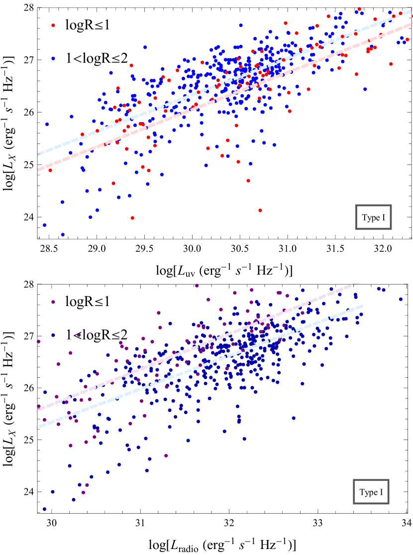
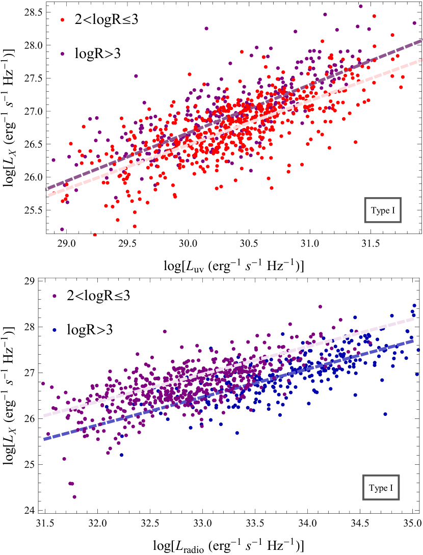
Figure 1: Plot of $\log{\kern 1.0pt}{L_{X}}vs.\log{\kern 1.0pt}{L_{uv}}$ (upper panel) and $\log{\kern 1.0pt}{L_{X}}vs.\log{\kern 1.0pt}{L_{radio}}$ (lower panel) for Type I quasars with different $logR$, the dotted line represents the theoretical values of $\log{\kern 1.0pt}{L_{X}}$ luminosity from the linear relation together with the best fitting values of parameters.

We firstly plot the ${L_{X}}-{L_{uv}}$ and ${L_{X}}-{L_{radio}}$ plane for Type I quasars and blazars (FSRLQs), as shown in Fig. 1 2, the luminosities ${L_{\lambda}}(2500{\AA})$ have been obtained from the measured fluxes assuming $\Lambda CDM$ cosmology $({\Omega_{m}}=0.3,{\kern 1.0pt}{\kern 1.0pt}{H_{0}}=70{\kern 1.0pt}km{\kern 1.0pt}{\kern 1.0pt}{s^{-1}}{\kern 1.0pt}Mp{c^{-1}})$. Meanwhile, we fit the linear relation to the data and obtain the theoretical values of X-Ray luminosity from the best fitting values of parameters. The upper left panel of Fig.1 illustrates the ${L_{X}}-{L_{uv}}$ plane for Type I quasars with $logR\leq 1$ (RQQs) and $1<logR\leq 2$ (RIQs), and the dotted line represents the theoretical values of X-Ray luminosity from the linear relation together with the best fitting values of parameters, which implies that the X-ray luminosity of RQQs and RIQs is related to UV-optical luminosity and originates from the inverse compton scattering. The lower left panel of Fig.1 shows the ${L_{X}}-{L_{radio}}$ plane for Type I RQQs and RIQs, and the dotted line represents the theoretical values, which also indicates that X-ray luminosity of RQQs is indirectly correlated with radio luminosity because of the connection between UV/optical and radio luminosity from Fig.3 (${L_{uv}}-{L_{radio}}$ plane). The indirect relation between X-Ray and radio luminosity in RQQs will also be discussed in Sec III.3.

Likewise, the ${L_{X}}-{L_{uv}}$ plane of Type I RLQs ($logR>2$) is shown in the upper right panel of Fig.1, which suggests that X-ray luminosity of RLQs is correlate with UV-optical luminosity. For the ${L_{X}}-{L_{radio}}$ plane of Type I RLQs illustrated in the lower right panel of Fig.1, whether or not the X-ray luminosity of RLQs is indirectly or directly related to radio luminosity will be discussed in Sec III.3.

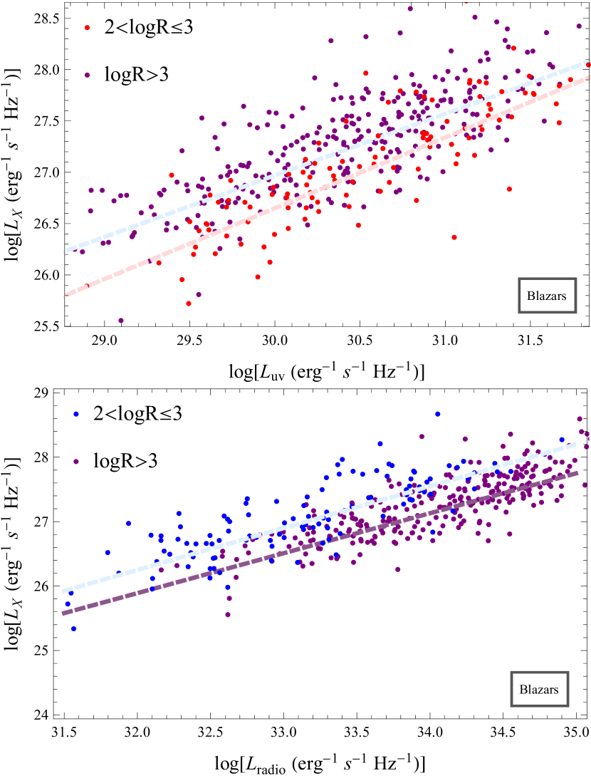
Figure 2: Plot of $\log{\kern 1.0pt}{L_{X}}vs.\log{\kern 1.0pt}{L_{uv}}$ (upper panel) and $\log{\kern 1.0pt}{L_{X}}vs.\log{\kern 1.0pt}{L_{radio}}$ (lower panel) for blazars (FSRLQs) with different $logR$, the dotted line represents the theoretical values of $\log{\kern 1.0pt}{L_{X}}$ luminosity from the linear relation together with the best fitting values of parameters.

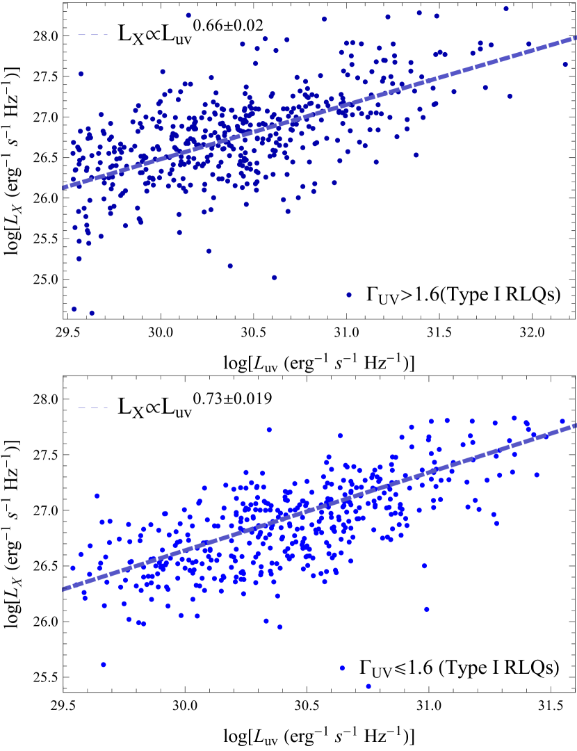
Figure 4: Plot of $\log{\kern 1.0pt}{L_{X}}vs.\log{\kern 1.0pt}{L_{uv}}$ for Type I quasars with ${\Gamma_{UV}}>1.6$ (upper panel) and ${\Gamma_{UV}}\leq 1.6$ (lower panel), the dotted line represents the theoretical values of $\log{\kern 1.0pt}{L_{X}}$ luminosity from the linear relation together with the best fitting values of parameters.

The ${L_{X}}-{L_{uv}}$ plane and ${L_{X}}-{L_{radio}}$ of blazars (FSRLQs) are illustrated in the upper and lower panel of Fig.2, which similarly implies that X-ray luminosity of RLQs is related to UV-optical luminosity. On the other hand, we compare the correlation between X-Ray luminosity and UV-optical luminosity of Type I quasars with UV-optical power-law ${\Gamma_{UV}}\leq 1.6$ and ${\Gamma_{UV}}>1.6$, which is shown in Fig.4. We will further discuss it in Sec III.3.

III.2 Models constraints from Type I quasars

We apply various parameterization methods to test the multi-band luminosity correlation of quasars, which involve different physical mechanisms. The most common parametric equation is [6, 7, 8, 9]

$$\begin{array}[]{l}Model\\ I:\log{L_{X}}=\alpha+{\gamma_{uv}}\log{L_{uv}}+\gamma_{radio}^{\prime}\log{L_{radio}},\end{array}$$ (3)

The above equation can become the relation ${L_{X}}\propto L_{uv}^{{\gamma_{uv}}}L_{radio}^{\gamma_{radio}^{\prime}}$, which concerns that X-ray luminosity is related to both UV-optical luminosity and radio luminosity. Using formula $L=4\pi{D_{L}}^{2}F$ in (3), we get

$$\begin{array}[]{l}\log{F_{X}}=\Phi({F_{UV}},{F_{radio}},{D_{L}})\\ {\kern 1.0pt}{\kern 1.0pt}{\kern 1.0pt}{\kern 1.0pt}{\kern 1.0pt}{\kern 1.0pt}{\kern 1.0pt}{\kern 1.0pt}{\kern 1.0pt}{\kern 1.0pt}{\kern 1.0pt}{\kern 1.0pt}{\kern 1.0pt}{\kern 1.0pt}{\kern 1.0pt}{\kern 1.0pt}{\kern 1.0pt}{\kern 1.0pt}{\kern 1.0pt}{\kern 1.0pt}{\kern 1.0pt}{\kern 1.0pt}{\kern 1.0pt}{\kern 1.0pt}{\kern 1.0pt}{\kern 1.0pt}{\kern 1.0pt}{\kern 1.0pt}{\kern 1.0pt}{\kern 1.0pt}{\kern 1.0pt}{\kern 1.0pt}{\kern 1.0pt}{\kern 1.0pt}=\alpha+{\gamma_{uv}}\log{F_{UV}}+\gamma_{radio}^{\prime}\log{F_{radio}}\\ {\kern 1.0pt}{\kern 1.0pt}{\kern 1.0pt}{\kern 1.0pt}{\kern 1.0pt}{\kern 1.0pt}{\kern 1.0pt}{\kern 1.0pt}{\kern 1.0pt}{\kern 1.0pt}{\kern 1.0pt}{\kern 1.0pt}{\kern 1.0pt}{\kern 1.0pt}{\kern 1.0pt}{\kern 1.0pt}{\kern 1.0pt}{\kern 1.0pt}{\kern 1.0pt}{\kern 1.0pt}{\kern 1.0pt}{\kern 1.0pt}{\kern 1.0pt}{\kern 1.0pt}{\kern 1.0pt}{\kern 1.0pt}{\kern 1.0pt}{\kern 1.0pt}{\kern 1.0pt}{\kern 1.0pt}{\kern 1.0pt}{\kern 1.0pt}{\kern 1.0pt}{\kern 1.0pt}+({\gamma_{uv}}+\gamma_{radio}^{\prime}-1)\log(4\pi{D_{L}}^{2}),\end{array}$$ (7)

where ${F_{X}}$, ${F_{UV}}$ and ${F_{radio}}$ are measured at (rest-frame) $2keV$, $2500Å$ and $5GHz$, $D_{L}$ is the luminosity distance, which can be obtained by the integral formula of $D_{L}-z$ relation. This equation can be effectively used for testing X-ray luminosity correlation for RLQs and RQQs.

The second model is considered that X-ray luminosity is only correlated with UV-optical luminosity, and its parametric form is [8, 30]

$$IV:{\kern 1.0pt}{\kern 1.0pt}{\kern 1.0pt}{\kern 1.0pt}{\kern 1.0pt}{\kern 1.0pt}\log{L_{X}}=\alpha+{\gamma_{uv}}\log{L_{uv}},$$ (8)

We can also consider other model as

$$III:{\kern 1.0pt}{\kern 1.0pt}{\kern 1.0pt}{\kern 1.0pt}{\kern 1.0pt}{\kern 1.0pt}\log{L_{X}}=\alpha+{\gamma_{radio}^{\prime}}\log{L_{radio}},$$ (9)

Model II and Model III can become the relation ${L_{X}}\propto L_{uv}^{{\gamma_{uv}}}$ and ${L_{X}}\propto L_{radio}^{\gamma_{radio}^{\prime}}$. The above two models refer that X-ray luminosity is only correlative with UV-optical or radio luminosity.

In the same way, from equations (8) and (9), we can get X-ray flux ${F_{X}}$ as the function of ${F_{UV}}$, ${F_{radio}}$ and $D_{L}$, which can be used to test X-ray luminosity relations.

We fit the three parametric models by minimizing a likelihood function consisting of a modified ${\chi^{2}}$ function based on MCMC, allowing for an intrinsic dispersion $\sigma$ [31]

$$\begin{array}[]{l}-2\ln L=\sum\limits_{i=1}^{N}{\left\{{\frac{{{{[\log{{({F_{X}})}_{i}}-\Phi{{({F_{UV}},{F_{radio}},{D_{L}})}_{i}}]}^{2}}}}{{s_{i}^{2}}}}\right\}}\\ {\kern 1.0pt}{\kern 1.0pt}{\kern 1.0pt}{\kern 1.0pt}{\kern 1.0pt}{\kern 1.0pt}{\kern 1.0pt}{\kern 1.0pt}{\kern 1.0pt}{\kern 1.0pt}{\kern 1.0pt}{\kern 1.0pt}{\kern 1.0pt}{\kern 1.0pt}{\kern 1.0pt}{\kern 1.0pt}{\kern 1.0pt}{\kern 1.0pt}{\kern 1.0pt}{\kern 1.0pt}{\kern 1.0pt}{\kern 1.0pt}{\kern 1.0pt}{\kern 1.0pt}{\kern 1.0pt}{\kern 1.0pt}{\kern 1.0pt}{\kern 1.0pt}{\kern 1.0pt}{\kern 1.0pt}{\kern 1.0pt}{\kern 1.0pt}{\kern 1.0pt}{\kern 1.0pt}{\kern 1.0pt}{\kern 1.0pt}{\kern 1.0pt}{\kern 1.0pt}+\sum\limits_{i=1}^{N}{\ln(2\pi s_{i}^{2})},\end{array}$$ (12)

where $\Phi({F_{UV}},{F_{radio}},{D_{L}})$ is given by equation (7), and $s_{i}^{2}=\sigma_{i}^{2}(\log{F_{X}})+\gamma_{uv}^{2}\sigma_{i}^{2}(\log{F_{UV}})+{\delta^{2}}$, $\delta$ is the intrinsic dispersion, which can be fitted as a free parameter and $\delta$ is usually much larger than the measurement error.

The Hubble constant ${H_{0}}$ is degenerate with the parameters $\alpha$ when fitting equation (7), we fix ${H_{0}}=70{\kern 1.0pt}{\kern 1.0pt}km{\kern 1.0pt}{\kern 1.0pt}{\kern 1.0pt}{s^{-1}}{\kern 1.0pt}Mp{c^{-1}}$ [32, 33]. If we want to better test X-ray luminosity relations and further select the optimal model, we should not fix ${\Omega_{m}}$. Therefore, we fit the three models to Type I quasars without fixing ${\Omega_{m}}$ and seek the best model.

We adopt the maximum likelihood function (equation (12)) based on MCMC to constrain three models, the model fitting results for Type I quasars are illustrated in Table 1. Meanwhile, we fit Model I to Type I quasars with ${\Gamma_{UV}}\leq 1.6$ and ${\Gamma_{UV}}>1.6$, as well as the objects with the X-Ray power-law index ${\Gamma_{X}}\leq 1.6$ and ${\Gamma_{X}}>1.6$, ${\Gamma_{X}}$ can be obtained from a fit of ${f_{\nu}}\propto{\nu^{-({\Gamma_{X}}-1)}}$ to their X-Ray fluxes(0.2-0.5, 0.5-1, 1-2, 4-4.5, 4.5-12 keV for XMM-Newtom and 0.5-1.2, 1.2-2, 2-7 keV for Chandra), the statistical results can be used to test whether there are different, which are also shown in Table 1.

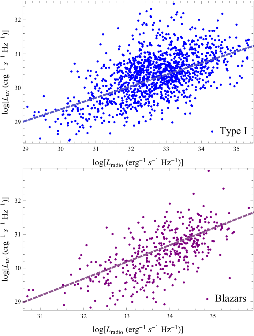
Figure 3: Plot of $\log{\kern 1.0pt}{L_{uv}}vs.\log{\kern 1.0pt}{L_{radio}}$ for Type I quasars (upper panel) and blazars (lower panel), the dotted line represents the theoretical values of $\log{\kern 1.0pt}{L_{X}}$ luminosity from the linear relation together with the best fitting values of parameters.

Table 1: Model fitting results for Type I RLQs and RQQs

Model	Sample	$\alpha$	${\gamma_{uv}}$	${\gamma_{radio}^{\prime}}$	$\delta$	${\Omega_{m}}$	$-2In{L_{\max}}/N$
I	$logR\leq 1$	4.12$\pm$1.47	0.323$\pm$0.038	0.4$\pm$0.075	0.65$\pm$0.049	0.514$\pm$0.078	185/97
	$1<logR\leq 2$	4.12$\pm$0.93	0.31$\pm$0.029	0.41$\pm$0.031	0.478$\pm$0.018	0.314$\pm$0.068	527/385
	$2<logR\leq 3$	5.09$\pm$0.652	0.442$\pm$0.028	0.253$\pm$0.025	0.281$\pm$0.009	0.094$\pm$0.091	144/492
	$logR>3$	4.5$\pm$0.8	0.517$\pm$0.044	0.202$\pm$0.028	0.3$\pm$0.014	0.195$\pm$0.025	89/218
	$logR>2;{\kern 1.0pt}{\Gamma_{UV}}\leq 1.6$	4.67$\pm$0.386	0.505$\pm$0.01	0.209$\pm$0.01	0.259$\pm$0.008	0.033$\pm$0.017	65/472
	$logR>2;{\kern 1.0pt}{\Gamma_{UV}}>1.6$	6.54$\pm$0.819	0.388$\pm$0.03	0.258$\pm$0.016	0.329$\pm$0.015	0.134$\pm$0.023	144/238
	$logR>2;{\kern 1.0pt}{\Gamma_{X}}\leq 1.6$	4.84$\pm$0.75	0.382$\pm$0.026	0.31$\pm$0.04	0.337$\pm$0.013	0.308$\pm$0.032	264.7/407
	$logR>2;{\kern 1.0pt}{\Gamma_{X}}>1.6$	8$\pm$0.52	0.4$\pm$0.021	0.2$\pm$0.02	0.29$\pm$0.013	0.347$\pm$0.1	89.3/256
II	$logR\leq 1$	6.53$\pm$0.774	0.652$\pm$0.025	$-$	0.64$\pm$0.047	0.545$\pm$0.108	186/97
	$1<logR\leq 2$	5.17$\pm$0.8	0.7$\pm$0.026	$-$	0.482$\pm$0.017	0.205$\pm$0.061	533/385
	$2<logR\leq 3$	5.99$\pm$0.658	0.687$\pm$0.022	$-$	0.288$\pm$0.009	0.035$\pm$0.019	174/492
	$logR>3$	5.19$\pm$0.97	0.719$\pm$0.032	$-$	0.307$\pm$0.015	0.188$\pm$0.079	100/218
III	$logR\leq 1$	6.08$\pm$0.813	$-$	0.652$\pm$0.026	0.661$\pm$0.056	0.4$\pm$0.191	193/97
	$1<logR\leq 2$	5.86$\pm$1	$-$	0.648$\pm$0.031	0.493$\pm$0.019	0.175$\pm$0.042	549/385
	$2<logR\leq 3$	7.8$\pm$0.933	$-$	0.578$\pm$0.029	0.299$\pm$0.017	0.213$\pm$0.054	203/492
	$logR>3$	8.52$\pm$0.427	$-$	0.547$\pm$0.013	0.325$\pm$0.016	0.343$\pm$0.052	127/218

Table 2: Measured properties of the 710 Type I RLQs, $DM$ are the distance modulus from a fit of the X-ray luminosity relation ${L_{X}}\propto L_{uv}^{{\gamma_{uv}}}L_{radio}^{\gamma_{radio}^{\prime}}$ with $\Lambda CDM$ model, ${\sigma_{DM}}$ are their error. ${\Gamma_{UV}}{\kern 1.0pt}or{\kern 1.0pt}{\kern 1.0pt}{\Gamma_{X}}=-99$ is used for cases of non-detection.

$SDSS{\kern 1.0pt}{\kern 1.0pt}{\kern 1.0pt}name$	$z$	${m_{i}}$	${F_{UV}}$	${F_{X}}$	${F_{radio}}$	$\log{\kern 1.0pt}{\kern 1.0pt}R$	${\Gamma_{UV}}$	${\Gamma_{X}}$	$DM$	${\sigma_{DM}}$
094334.00+463332.1	3.216	20.401$\pm$0.026	-24.149$\pm$0.010	-27.739$\pm$0	-20.859	3.29	2.004	-99	47.798	2.444
090237.33+010135.9	3.12	20.601$\pm$0.041	-24.184$\pm$0.016	-27.803$\pm$0.054	-21.58	2.603	1.856	0.921	46.841	2.407
104909.81+373759.0	3.003	18.075$\pm$0.082	-23.167$\pm$0.033	-27.049$\pm$0.008	-20.833	2.333	3.769	1.382	45.854	2.370
160421.77+432354.6	2.408	19.389$\pm$0.015	-23.658$\pm$0.006	-27.023$\pm$0.007	-20.634	3.023	1.437	1.388	44.311	2.297
084218.39+362504.2	2.244	19.265$\pm$0.021	-23.597$\pm$0.008	-27.014$\pm$0.022	-20.81	2.786	1.853	1.435	44.124	2.304

Table 3: Fit results on model parameters for a combination of SNla and Type I RLQs

	$Sample$	$\alpha$	${\gamma_{uv}}$	$\gamma_{radio}^{\prime}$	$\delta$	${\Omega_{m}}$	${w_{0}}$	${w_{\alpha}}$	$\chi_{Total}^{2}$/${\chi^{\prime}}_{Total}^{2}$/N
$\Lambda CDM$	RLQs	5.29$\pm$0.212	0.44$\pm$0.01	0.25$\pm$0.012	0.283$\pm$0.008	0.176$\pm$0.013	$-$	$-$	232.8/708/710
	SN+RLQs	6.155$\pm$0.388	0.434$\pm$0.019	0.227$\pm$0.01	0.285$\pm$0.007	0.271$\pm$0.007	$-$	$-$	1272.4/1746.6/1758
	SN+RLQs (${\Gamma_{UV}}\leq 1.6$)	5.6$\pm$0.339	0.442$\pm$0.013	0.224$\pm$0.011	0.261$\pm$0.008	0.273$\pm$0.008	$-$	$-$	1107.6/1506.6/1520
	SN+RLQs (${\Gamma_{UV}}>1.6$)	4.89$\pm$0.557	0.437$\pm$0.025	0.262$\pm$0.02	0.33$\pm$0.015	0.273$\pm$0.007	$-$	$-$	1182.5/1271.1/1286
${w_{0}}{w_{a}}CDM$	SN+RLQs	5.68$\pm$0.255	0.434$\pm$0.009	0.24$\pm$0.006	0.285$\pm$0.008	0.298$\pm$0.012	-1.107$\pm$0.044	0.412$\pm$0.366	1269.2/1743.4/1758
	SN+RLQs (${\Gamma_{UV}}\leq 1.6$)	5.95$\pm$0.358	0.453$\pm$0.021	0.216$\pm$0.024	0.261$\pm$0.008	0.29$\pm$0.016	-1.09$\pm$0.04	0.41$\pm$0.335	1104.7/1503.7/1520
	SN+RLQs (${\Gamma_{UV}}>1.6$)	5.25$\pm$0.389	0.426$\pm$0.019	0.261$\pm$0.014	0.33$\pm$0.016	0.286$\pm$0.027	-1.126$\pm$0.075	0.757$\pm$0.306	1178.8/1267.3/1286

III.3 Models analysis and comparison

We use BIC to seek an optimal model. The BIC is

$$BIC=-2\ln{L_{\max}}+k{\kern 1.0pt}{\kern 1.0pt}\ln{\kern 1.0pt}{\kern 1.0pt}N,$$ (13)

where ${L_{\max}}$ is the maximum likelihood, $k$ is the number of free parameters of the model, and $N$ is the number of data points.

For model II, by comparing the results in Tabel 1 from different logR of Type I quasars, we find that the correlation between X-ray and UV-optical luminosity increases with logR. Similarly, for the model I, the statistical results imply that the correlation between X-ray and radio luminosity becomes stronger as the ratio of monochromatic luminosities logR increases. Meanwhile, Model II has the smallest BIC by comparing the results in Table 1 from fitting for different models to RQQs, which indicates that the X-ray luminosity of RQQs is not directly correlated with their radio luminosity, but there is an indirect relation between X-ray and radio luminosity because of the connection between UV-optical and radio luminosity from Fig. 3.

For RLQs, BIC for Model I is far smaller than Model II and III, which implies X-ray luminosity of RLQs is not only connected with optical/UV luminosity but also directly related to radio luminosity. A possible reason for the luminosity correlations RLQs is that a fraction of the nuclear X-ray emission is directly or indirectly powered by the radio jet, the specific physical mechanism needs to be further understood.

As for RIQs, By comparing BIC in Table 1 from fitting for different models to RIQs, we find that Model I has the smallest BIC, which might indicate that there is a weak correlation between the X-ray and radio luminosity of RIQs. Furthermore, for the fitting results BIC, there is a difference between Type I quasars with ${\Gamma_{UV}}\leq 1.6$ and ${\Gamma_{UV}}>1.6$ for Model I, the same goes for ${\Gamma_{X}}\leq 1.6$ and ${\Gamma_{X}}>1.6$. The goodness of fit for ${\Gamma_{UV}}\leq 1.6$ and ${\Gamma_{X}}>1.6$ seem to be better.

III.4 Analysis of the relation ${L_{X}}\propto L_{uv{\kern 1.0pt}{\kern 1.0pt}}^{{\gamma_{uv}}}L_{radio{\kern 1.0pt}{\kern 1.0pt}}^{\gamma_{radio}^{\prime}}$

We divide the Type I RLQs sample in several redshift bins, which can be used to verify if there is redshift dependence for luminosity relation. The redshift bin are $\Delta({(1+z)^{-1}})=0.05$. We apply the parametric model [31]

$$\begin{array}[]{l}\log{F_{X}}=\alpha(z)+{\gamma_{uv}}(z)\log{F_{UV}}\\ {\kern 1.0pt}{\kern 1.0pt}{\kern 1.0pt}{\kern 1.0pt}{\kern 1.0pt}{\kern 1.0pt}{\kern 1.0pt}{\kern 1.0pt}{\kern 1.0pt}{\kern 1.0pt}{\kern 1.0pt}{\kern 1.0pt}{\kern 1.0pt}{\kern 1.0pt}{\kern 1.0pt}{\kern 1.0pt}{\kern 1.0pt}{\kern 1.0pt}{\kern 1.0pt}{\kern 1.0pt}{\kern 1.0pt}{\kern 1.0pt}{\kern 1.0pt}{\kern 1.0pt}{\kern 1.0pt}{\kern 1.0pt}{\kern 1.0pt}{\kern 1.0pt}{\kern 1.0pt}{\kern 1.0pt}{\kern 1.0pt}{\kern 1.0pt}+{\gamma_{radi{o^{\prime}}}}(z)\log{F_{radio}},\end{array}$$ (16)

where $\alpha(z),{\kern 1.0pt}{\gamma_{uv}}(z),{\kern 1.0pt}\gamma_{radio}^{\prime}(z)$ and the intrinsic dispersion $\delta(z)$ are free parameters. We fit equation (16) to segmented Type I RLQs and check whether the X-Rays relation is dependent on the redshift. The fit results of ${\gamma_{uv}}(z),{\kern 1.0pt}{\kern 1.0pt}\gamma_{radio}^{\prime}(z),and{\kern 1.0pt}{\kern 1.0pt}\delta(z)$ at different redshift are illustrated in Fig. 5, which show that their values are no obvious evidence for any significant redshift evolution. The average values of parameters are $\left\langle{{\gamma_{uv}}}\right\rangle=0.47\pm 0.1,{\kern 1.0pt}{\kern 1.0pt}{\kern 1.0pt}\left\langle{\gamma_{radio}^{\prime}}\right\rangle=0.27\pm 0.056.$

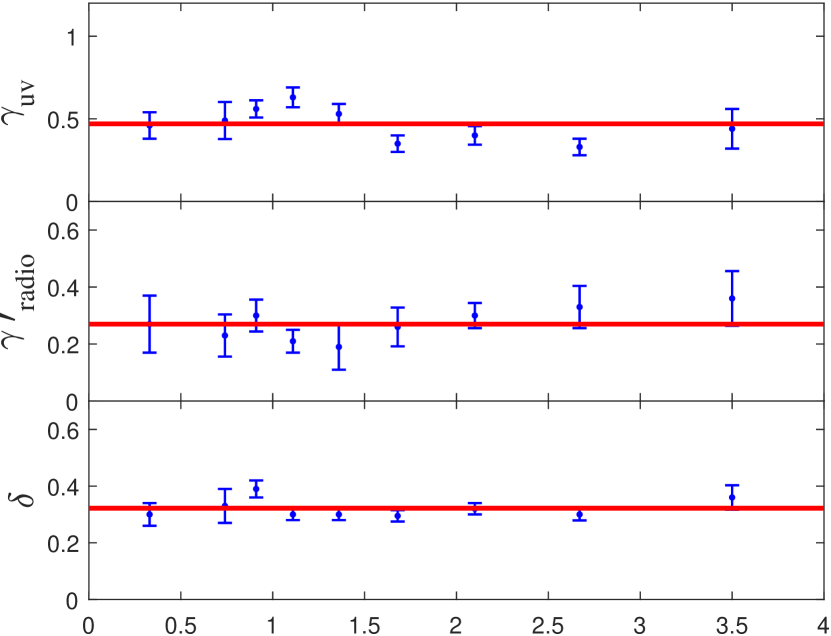
Figure 5: ${L_{X}}-{L_{uv}}/{L_{radio}}$ correlation in narrow redshift intervals. Blue points represent fitted values and errors of ${\gamma_{UV}}(z),{\kern 1.0pt}{\kern 1.0pt}\gamma_{radio}^{\prime}(z),{\kern 1.0pt}{\kern 1.0pt}\sigma(z)$ at different redshift. The horizontal lines are their average values.

IV A measure of luminosity distance for Type I RLQs

Meanwhile, we measure the luminosity distance for Type I RLQs. From Model I, equation (7) gives distance modulus as

$$DM=\frac{{5[\log{F_{X}}-{\gamma_{uv}}\log{F_{UV}}-\gamma_{radio}^{\prime}{F_{radio}}-{\alpha^{\prime}}]}}{{2({\gamma_{uv}}+\gamma_{radio}^{\prime}-1)}},$$ (17)

where ${\alpha^{\prime}}=\alpha+({\gamma_{uv}}+\gamma_{radio}^{\prime}-1)\log(4\pi)$. The formula of error is

$${\sigma_{DM}}=DM\sqrt{{{(\frac{{{\sigma_{f}}}}{f})}^{2}}+{{(\frac{{{\sigma_{{\gamma_{uv}}}}}}{\gamma})}^{2}}+{{(\frac{{{\sigma_{{\gamma_{radio}^{\prime}}}}}}{\gamma})}^{2}}}.$$ (18)

where $f={\log{F_{X}}-{\gamma_{uv}}\log{F_{UV}}-{{\gamma^{\prime}}_{radio}}{F_{radio}}-\alpha^{\prime}}$, $\gamma={\gamma_{uv}}+{\gamma_{radio}^{\prime}}-1$, and ${\sigma_{f}}^{2}=\sigma_{i}^{2}(\log{F_{X}})+\gamma_{uv}^{2}\sigma_{i}^{2}(\log{F_{UV}})+\sigma_{\alpha^{\prime}}^{2}$. From equation (18), the uncertainty of the slope ${\gamma_{uv}}$ and $\gamma_{radio}^{\prime}$ obviously influence the error of distance modulus for Type I RLQs.

Fig 6 shows distance modulus of Type I quasars with ${\Gamma_{UV}}\leq 1.6$ and ${\Gamma_{UV}}>1.6$ from a fit of Model I when assuming $\Lambda CDM$ cosmology, and their averages in small redshift bins. Meanwhile the properties of 710 Type I quasars and their distance modulus are listed in Table 2.

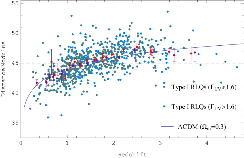
Figure 6: The distance modulus of Type I quasars with ${\Gamma_{X}}\leq 1.6$ and ${\Gamma_{X}}>1.6$ from a fit of Equation (7) when assuming $\Lambda CDM$ cosmology. The purple and red points are distance modulus averages in small redshift bins. The blue line shows a flat $\Lambda CDM$ model fit with ${\Omega_{m}}=0.3$, the dotted line is the reference distance modulus and its value is 45.

V The reconstruction of dark energy equation of state w(z)

Although the dark energy model can be used to effectively explain the accelerating expansion of the universe and the cosmic microwave background (CMB) anisotropies [34, 35, 36, 37, 38, 33, 39, 40, 41, 42], the origin and property of dark energy density and pressure are still unclear.

The research methods of dark energy include two kinds. One is to try to explain the physical origin of its density and pressure by constraining dark energy physical models [43, 44, 45, 46, 47]. Understanding the physical nature of dark energy is important for our universe. Whether or not the dark energy is composed of Fermion pairs in a vacuum or Boson pairs, Higgs field. The order of magnitude for the strength of dark energy is far smaller than that the elementary particles needed when they were created in the very early Universe. The other method is to investigate whether or not the dark energy density evolves with time, this can be checked by reconstructing the dark energy equation of state $w(z)$ [48, 49], which is independent of physical models. The high redshift observational data can better solve these problems.

The reconstruction methods of the dark energy equation of state can be classed into parametric and non-parametric methods [50, 51, 52, 53, 54, 55, 56, 57, 58]. We apply Type I RLQs and SNla to reconstruct $w(z)$ by parametric method assuming X-ray luminosity relation Equation (7), which can be used for testing the property of dark energy.

SNla Pantheon sample is a combination of data sources from the Sloan Digital Sky Survey (SDSS), the Pan-STARRS1 (PS1), SNLS, and various low-z and Hubble Space Telescope samples. There are 335 SNIa provided by SDSS [36, 59, 60, 61, 62], and PS1 presented 279 SNla [37]. The rest of the Pantheon sample are from the ${\rm{CfA1-4}}$, CSP, and Hubble Space Telescope (HST) SN surveys [35, 38]. This joint sample of 1048 SNIa is called the Pantheon sample.

The integral formula of ${D_{L}}-z$ relation in near flat space is given by

$$\begin{array}[]{l}{D_{L}}=\frac{{1+z}}{{{H_{0}}}}\int_{0}^{z}{d{z^{\prime}}[{\Omega_{m}}{{(1+{z^{\prime}})}^{3}}}\\ {\kern 1.0pt}{\kern 1.0pt}{\kern 1.0pt}{\kern 1.0pt}{\kern 1.0pt}{\kern 1.0pt}{\kern 1.0pt}{\kern 1.0pt}{\kern 1.0pt}{\kern 1.0pt}{\kern 1.0pt}{\kern 1.0pt}{\kern 1.0pt}{\kern 1.0pt}{\kern 1.0pt}{\kern 1.0pt}{\kern 1.0pt}{\kern 1.0pt}{\kern 1.0pt}{\kern 1.0pt}{\kern 1.0pt}{\kern 1.0pt}{\kern 1.0pt}{\kern 1.0pt}{\kern 1.0pt}{\kern 1.0pt}{\kern 1.0pt}{\kern 1.0pt}{\kern 1.0pt}{\kern 1.0pt}{\kern 1.0pt}{\kern 1.0pt}{\kern 1.0pt}{\kern 1.0pt}{\kern 1.0pt}{\kern 1.0pt}{\kern 1.0pt}{\kern 1.0pt}{\kern 1.0pt}{\kern 1.0pt}{\kern 1.0pt}{\kern 1.0pt}{\kern 1.0pt}{\kern 1.0pt}{\kern 1.0pt}{\kern 1.0pt}{\kern 1.0pt}{\kern 1.0pt}{\kern 1.0pt}{\kern 1.0pt}{\kern 1.0pt}+{\Omega_{R}}{(1+{z^{\prime}})^{4}}+\Omega_{DE}^{(0)}{{\mathop{\rm e}\nolimits}^{\int_{0}^{{z^{\prime}}}{\frac{{1+w({z^{{}^{\prime\prime}}})}}{{1+{z^{{}^{\prime\prime}}}}}d{z^{{}^{\prime\prime}}}}}}{]^{-1/2}}\end{array}$$ (19)

where ${{\Omega_{R}}}$ is radiation density. ${\Omega_{DE}^{(0)}}$ is the present dark energy density and satisfies $\Omega_{DE}^{(0)}=1-{\Omega_{m}}$ when ignoring ${{\Omega_{R}}}$, $w(z)$ is dark energy equation of state. We choose ${w_{0}}{w_{a}}CDM$ model and the parametric form is

$$w(z)={w_{0}}+{w_{a}}\frac{z}{{1+z}}.$$ (20)

Therefore dark energy density can be written as

$${\Omega_{DE}}(z)=\Omega_{DE}^{(0)}{(1+z)^{3(1+{w_{0}}+{w_{a}})}}\exp[-3{w_{a}}z/(1+z)].$$ (21)

We fit ${{\rm{w}}_{0}}{{\rm{w}}_{a}}{\rm{CDM}}$ model parameters to Type I RLQs and SNla by minimizing $\chi_{Total}^{2}$, the $\chi_{Total}^{2}$ is

$$\chi_{Total}^{2}=-2\ln{L^{RLQs}}+\chi_{SN}^{2},$$ (22)

where $-2\ln{L^{RLQs}}$ is given by equation (12), and $\chi_{SN}^{2}$ can be expressed as

$$\chi_{SN}^{2}=\Delta{\mu^{T}}C_{{\mu_{ob}}}^{-1}\Delta\mu,$$ (23)

where $\Delta\mu=\mu-{\mu_{th}}$. ${C_{\mu}}$ is the covariance matrix of the distance modulus $\mu$. Another function is ${\chi^{\prime}}_{Total}^{2}$, which satisfies

$${\chi^{\prime}}_{Total}^{2}=\chi_{RLQs}^{2}+\chi_{SN}^{2},$$ (24)

and $\chi_{RLQs}^{2}=-2\ln{L^{RLQs}}-\sum\limits_{i=1}^{N}{\ln(2\pi s_{i}^{2})}$.

We adopt equation (22) to constrain model parameters, and fit results are illustrated in table 3, ${w_{0}}{w_{a}}CDM$ has better goodness of fit than $\Lambda CDM$, and $\Delta\chi_{Total}^{2}$ is improved by $-3.2$, it implies $\Lambda CDM$ model is in tension with Type I RLQs at $\sim 1.5\sigma$, which is consistent with the results from the distance measurement using Baldwin effect of quasars [1, 63]. Meanwhile fig 7 shows $68\%$ and $95\%$ contours for ${w_{0}}$ and ${w_{a}}$ from a fit of the X-ray luminosity relation ${L_{X}}\propto L_{uv}^{{\gamma_{uv}}}L_{radio}^{\gamma_{radio}^{\prime}}$ and ${{\rm{w}}_{0}}{{\rm{w}}_{a}}{\rm{CDM}}$ model to a combination of SNla and Type I RLQs.

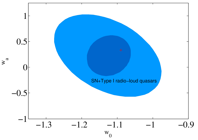
Figure 7: $68\%$ and $95\%$ contours for ${w_{0}}$ and ${w_{a}}$ from a fit of the X-ray luminosity relation ${L_{X}}\propto L_{uv}^{{\gamma_{uv}}}L_{radio}^{\gamma_{radio}^{\prime}}$ with $\Lambda CDM$ and ${w_{0}}{w_{a}}CDM$ model to a combination of SNla and Type I RLQs. The + dot in the responding color represents the best fitting values for ${w_{0}}$, ${w_{a}}$.

VI Summary

The investigation of X-ray luminosity correlation for RQQs and RLQs could make us understand more of their physical mechanism. We obtain a new sample of 1192 Type I quasars with the UV-optical, radio and X-ray wavebands coverage by combining Huang and Chang [1] and other matching data of SDSS-DR16 with FIRST, XMM–Newton, and Chandra Source Catalog, and a sample of 407 flat-spectrum radio-loud quasars (FSRLQs) of blazars from the Roma-BZCAT. Firstly, we apply three parametric methods to test the correlation between X-ray, UV-optical, and radio luminosity. The statistical results indicate that the X-ray luminosity of RQQs is correlated with their UV-optical luminosity, which also can be considered that the X-ray luminosity of RQQs is indirectly correlated with radio luminosity because of the connection between UV-optical and radio luminosity.

Meanwhile, data suggest that the correlation between X-ray and UV-optical luminosity increases with the ratio of monochromatic luminosities $logR$, Similarly, the correlation between X-ray and radio luminosity also becomes stronger as $logR$ increases. For RLQs, the results imply that the X-ray luminosity of RLQs is not only connected with optical/UV luminosity but also directly related to radio luminosity. A possible reason for the luminosity correlations RLQs is that a fraction of the nuclear X-ray emission is directly or indirectly powered by the radio jet. In addition, we compare the results from Type I quasars with ${\Gamma_{UV}}\leq 1.6$ and ${\Gamma_{UV}}>1.6$, as well as ${\Gamma_{X}}\leq 1.6$ and ${\Gamma_{X}}>1.6$ using a fit of X-ray luminosity relation ${L_{X}}\propto L_{uv}^{{\gamma_{uv}}}L_{radio}^{\gamma_{radio}^{\prime}}$, the goodness of fit for ${\Gamma_{UV}}\leq 1.6$ and ${\Gamma_{X}}>1.6$ seem to be better.

Secondly, We divide the Type I RLQs sample into discrete redshift bins and combine a special model, which can be applied to describe if there is a redshift evolution of X-ray luminosity relation ${L_{X}}\propto L_{uv}^{{\gamma_{uv}}}L_{radio}^{\gamma_{radio}^{\prime}}$, the fit results show the model parameters approach to the constant, which indicates there is not an obvious redshift dependence for ${L_{X}}\propto L_{uv}^{{\gamma_{uv}}}L_{radio}^{\gamma_{radio}^{\prime}}$.

Finally, we obtain the luminosity distance of 710 Type I RLQs from a fit of X-ray luminosity relation ${L_{X}}\propto L_{uv}^{{\gamma_{uv}}}L_{radio}^{\gamma_{radio}^{\prime}}$ when assuming $\Lambda CDM$ cosmology, and use a joint of SNla and Type I RLQs sample to reconstruct the dark energy equation of state $w(z)$ by parametric method and test the nature of dark energy. The data suggests ${w_{0}}{w_{a}}CDM$ model is superior to cosmological constant $\Lambda CDM$ model at $\sim 1.5\sigma$.

In the future, we will cross-correlate the Dark Energy Spectroscopic Instrument (DESI) quasar catalogs with the XMM-Newton, Chandra archives, and radio surveys. We expect to obtain more quasars with multi-wavelength coverage and high redshift ($z>3$) objects, which can be used to investigate their multi-band luminosity correlations. Meanwhile, the high redshift observational data can better test the properties of dark energy, it will determine the future of the universe, whether the universe keeps expanding or shifts from expansion to contraction. It will similarly determine the future of humanity.

References

- Huang and Chang [2022] L. Huang and Z. Chang, MNRAS 515, 1358 (2022).
- Strittmatter et al. [1980] P. Strittmatter, P. Hill, I. Pauliny-Toth, H. Steppe, and A. Witzel, A&A 88, L12 (1980).
- Kellermann et al. [1989] K. Kellermann, R. Sramek, M. Schmidt, D. Shaffer, and R. Green, AJ 98, 1195 (1989).
- Stocke et al. [1992] J. T. Stocke, S. L. Morris, R. J. Weymann, and C. B. Foltz, APJ 396, 487 (1992).
- Kellermann et al. [1994] K. Kellermann, R. Sramek, M. Schmidt, R. Green, and D. Shaffer, AJ 108, 1163 (1994).
- Tananbaum et al. [1983] H. Tananbaum, J. Wardle, G. Zamorani, and Y. Avni, APJ 268, 60 (1983).
- Worrall et al. [1987] D. Worrall, P. Giommi, H. Tananbaum, and G. Zamorani, APJ 313, 596 (1987).
- Miller et al. [2010] B. P. Miller, W. Brandt, D. Schneider, R. Gibson, A. Steffen, and J. Wu, APJ 726, 20 (2010).
- Zhu et al. [2020] S. Zhu, W. Brandt, B. Luo, J. Wu, Y. Xue, and G. Yang, MNRAS 496, 245 (2020).
- Browne and Murphy [1987] I. Browne and D. Murphy, MNRAS 226, 601 (1987).
- Evans et al. [2006] D. Evans, D. Worrall, M. Hardcastle, R. Kraft, and M. Birkinshaw, APJ 642, 96 (2006).
- Hardcastle et al. [2009] M. Hardcastle, D. Evans, and J. Croston, MNRAS 396, 1929 (2009).
- Urry and Padovani [1995] C. M. Urry and P. Padovani, Publ. Astron. Soc. Aust. 107, 803 (1995).
- Sulentic et al. [2000] J. Sulentic, P. Marziani, and D. Dultzin-Hacyan, ARA&A 38, 521 (2000).
- D’Abrusco et al. [2014] R. D’Abrusco, F. Massaro, A. Paggi, H. Smith, N. Masetti, M. Landoni, and G. Tosti, APJS 215, 14 (2014).
- D’Abrusco et al. [2019] R. D’Abrusco, N. Á. Crespo, F. Massaro, R. Campana, V. Chavushyan, M. Landoni, F. La Franca, N. Masetti, D. Milisavljevic, A. Paggi, et al., APJS 242, 4 (2019).
- Lyke et al. [2020] B. W. Lyke, A. N. Higley, J. McLane, D. P. Schurhammer, A. D. Myers, A. J. Ross, K. Dawson, S. Chabanier, P. Martini, H. D. M. Des Bourboux, et al., APJS 250, 8 (2020).
- Ahumada et al. [2020] R. Ahumada, C. A. Prieto, A. Almeida, F. Anders, S. F. Anderson, B. H. Andrews, B. Anguiano, R. Arcodia, E. Armengaud, M. Aubert, et al., APJS 249, 3 (2020).
- Pâris et al. [2017] I. Pâris, P. Petitjean, N. P. Ross, A. D. Myers, É. Aubourg, A. Streblyanska, S. Bailey, É. Armengaud, N. Palanque-Delabrouille, C. Yèche, et al., A&A 597, A79 (2017).
- Alam et al. [2015] S. Alam, F. D. Albareti, C. A. Prieto, F. Anders, S. F. Anderson, T. Anderton, B. H. Andrews, E. Armengaud, É. Aubourg, S. Bailey, et al., APJS 219, 12 (2015).
- Richards et al. [2002] G. T. Richards, X. Fan, H. J. Newberg, M. A. Strauss, D. E. V. Berk, D. P. Schneider, B. Yanny, A. Boucher, S. Burles, J. A. Frieman, et al., AJ 123, 2945 (2002).
- Helfand et al. [2015] D. J. Helfand, R. L. White, and R. H. Becker, APJ 801, 26 (2015).
- Rosen et al. [2016] S. Rosen, N. Webb, M. Watson, J. Ballet, D. Barret, V. Braito, F. Carrera, M. Ceballos, M. Coriat, R. Della Ceca, et al., A&A 590, A1 (2016).
- Webb et al. [2020] N. Webb, M. Coriat, I. Traulsen, J. Ballet, C. Motch, F. J. Carrera, F. Koliopanos, J. Authier, I. de La Calle, M. T. Ceballos, et al., A&A 641, A136 (2020).
- Evans et al. [2010] I. N. Evans, F. A. Primini, K. J. Glotfelty, C. S. Anderson, N. R. Bonaventura, J. C. Chen, J. E. Davis, S. M. Doe, J. D. Evans, G. Fabbiano, et al., APJS 189, 37 (2010).
- Richards et al. [2006] G. T. Richards, M. Lacy, L. J. Storrie Lombardi, P. B. Hall, S. Gallagher, D. C. Hines, X. Fan, C. Papovich, D. E. V. Berk, G. B. Trammell, et al., APJS 166, 470 (2006).
- Massaro et al. [2009] E. Massaro, P. Giommi, C. Leto, P. Marchegiani, A. Maselli, M. Perri, S. Piranomonte, and S. Sclavi, A&A 495, 691 (2009).
- Massaro et al. [2012] E. Massaro, R. Nesci, and S. Piranomonte, MNRAS 422, 2322 (2012).
- Massaro et al. [2015] E. Massaro, A. Maselli, C. Leto, P. Marchegiani, M. Perri, P. Giommi, and S. Piranomonte, ASTROPHYS SPACE SCI 357, 1 (2015).
- Bisogni et al. [2021] S. Bisogni, E. Lusso, F. Civano, E. Nardini, G. Risaliti, M. Elvis, and G. Fabbiano, A&A 655, A109 (2021).
- Risaliti and Lusso [2015] G. Risaliti and E. Lusso, APJ 815, 33 (2015).
- Reid et al. [2019] M. Reid, D. W. Pesce, and A. Riess, APJL 886, L27 (2019).
- Aghanim et al. [2020] N. Aghanim, Y. Akrami, M. Ashdown, J. Aumont, C. Baccigalupi, M. Ballardini, A. Banday, R. Barreiro, N. Bartolo, S. Basak, et al., A&A 641, A6 (2020).
- Riess et al. [1998] A. G. Riess, A. V. Filippenko, P. Challis, A. Clocchiatti, A. Diercks, P. M. Garnavich, R. L. Gilliland, C. J. Hogan, S. Jha, R. P. Kirshner, et al., AJ 116, 1009 (1998).
- Amanullah et al. [2010] R. Amanullah, C. Lidman, D. Rubin, G. Aldering, P. Astier, K. Barbary, M. Burns, A. Conley, K. Dawson, S. Deustua, et al., APJ 716, 712 (2010).
- Betoule et al. [2014] M. Betoule, R. Kessler, J. Guy, J. Mosher, D. Hardin, R. Biswas, P. Astier, P. El-Hage, M. Konig, S. Kuhlmann, et al., A&A 568, A22 (2014).
- Scolnic et al. [2018] D. M. Scolnic, D. Jones, A. Rest, Y. Pan, R. Chornock, R. Foley, M. Huber, R. Kessler, G. Narayan, A. Riess, et al., APJ 859, 101 (2018).
- Conley et al. [2010] A. Conley, J. Guy, M. Sullivan, N. Regnault, P. Astier, C. Balland, S. Basa, R. Carlberg, D. Fouchez, D. Hardin, et al., APJS 192, 1 (2010).
- Hu and Dodelson [2002] W. Hu and S. Dodelson, ARA&A 40, 171 (2002).
- Spergel et al. [2003] D. N. Spergel, L. Verde, H. V. Peiris, E. Komatsu, M. Nolta, C. L. Bennett, M. Halpern, G. Hinshaw, N. Jarosik, A. Kogut, et al., APJS 148, 175 (2003).
- Ade et al. [2016] P. Ade, N. Aghanim, M. Arnaud, M. Ashdown, J. Aumont, C. Baccigalupi, A. Banday, R. Barreiro, J. Bartlett, N. Bartolo, et al., A&A 594, A24 (2016).
- Aghanim et al. [2016] N. Aghanim, M. Ashdown, J. Aumont, C. Baccigalupi, M. Ballardini, A. Banday, R. Barreiro, N. Bartolo, S. Basak, R. Battye, et al., A&A 596, A107 (2016).
- Peebles and Ratra [2003] P. J. E. Peebles and B. Ratra, Rev. Mod. Phys 75, 559 (2003).
- Ratra and Peebles [1988] B. Ratra and P. J. Peebles, Phys. Rev. D 37, 3406 (1988).
- Li [2004] M. Li, Phys. Lett. B 603, 1 (2004).
- Maziashvili [2007] M. Maziashvili, Int. J. Mod. Phys. D 16, 1531 (2007).
- Amendola [2000] L. Amendola, Phys. Rev. D 62, 043511 (2000).
- Linder [2003] E. V. Linder, Phys. Rev. Lett. 90, 091301 (2003).
- Maor et al. [2002] I. Maor, R. Brustein, J. McMahon, and P. J. Steinhardt, Phys. Rev. D 65, 123003 (2002).
- Huterer and Starkman [2003] D. Huterer and G. Starkman, Phys. Rev. Lett. 90, 031301 (2003).
- Clarkson and Zunckel [2010] C. Clarkson and C. Zunckel, Phys. Rev. Lett. 104, 211301 (2010).
- Holsclaw et al. [2010] T. Holsclaw, U. Alam, B. Sanso, H. Lee, K. Heitmann, S. Habib, and D. Higdon, Phys. Rev. Lett. 105, 241302 (2010).
- Seikel et al. [2012] M. Seikel, C. Clarkson, and M. Smith, J. Cosmol. Astropart. Phys. 2012 (06), 036.
- Shafieloo et al. [2012] A. Shafieloo, A. G. Kim, and E. V. Linder, Phys. Rev. D 85, 123530 (2012).
- Crittenden et al. [2012] R. G. Crittenden, G.-B. Zhao, L. Pogosian, L. Samushia, and X. Zhang, J. Cosmol. Astropart. Phys. 2012 (02), 048.
- Zhao et al. [2012] G.-B. Zhao, R. G. Crittenden, L. Pogosian, and X. Zhang, Phys. Rev. Lett. 109, 171301 (2012).
- Fu et al. [2019] X. Fu, L. Zhou, and J. Chen, Phys. Rev. D 99, 083523 (2019).
- Cao et al. [2017] S. Cao, X. Zheng, M. Biesiada, J. Qi, Y. Chen, and Z.-H. Zhu, A& A 606, A15 (2017).
- Gunn et al. [2006] J. E. Gunn, W. A. Siegmund, E. J. Mannery, R. E. Owen, C. L. Hull, R. F. Leger, L. N. Carey, G. R. Knapp, D. G. York, W. N. Boroski, et al., AJ 131, 2332 (2006).
- Gunn et al. [1998] J. Gunn, M. Carr, C. Rockosi, M. Sekiguchi, K. Berry, B. Elms, E. De Haas, Ž. Ivezić, G. Knapp, R. Lupton, et al., AJ 116, 3040 (1998).
- Sako et al. [2007] M. Sako, B. Bassett, A. Becker, D. Cinabro, F. DeJongh, D. L. Depoy, B. Dilday, M. Doi, J. A. Frieman, P. M. Garnavich, et al., AJ 135, 348 (2007).
- Sako et al. [2018] M. Sako, B. Bassett, A. C. Becker, P. J. Brown, H. Campbell, R. Wolf, D. Cinabro, C. B. D’andrea, K. S. Dawson, F. DeJongh, et al., Publ. Astron. Soc. Aust. 130, 064002 (2018).
- Huang et al. [2023] L. Huang, H. Wang, Z. Gao, X. Zeng, and Z. Chang, A& A 674, A163 (2023).