Sparsified Simultaneous Confidence Intervals for High-Dimensional Linear Models

Abstract

Statistical inference of the high-dimensional regression coefficients is challenging because the uncertainty introduced by the model selection procedure is hard to account for. A critical question remains unsettled; that is, is it possible and how to embed the inference of the model into the simultaneous inference of the coefficients? To this end, we propose a notion of simultaneous confidence intervals called the sparsified simultaneous confidence intervals. Our intervals are sparse in the sense that some of the intervals’ upper and lower bounds are shrunken to zero (i.e., $[0,0]$), indicating the unimportance of the corresponding covariates. These covariates should be excluded from the final model. The rest of the intervals, either containing zero (e.g., $[-1,1]$ or $[0,1]$) or not containing zero (e.g., $[2,3]$), indicate the plausible and significant covariates, respectively. The proposed method can be coupled with various selection procedures, making it ideal for comparing their uncertainty. For the proposed method, we establish desirable asymptotic properties, develop intuitive graphical tools for visualization, and justify its superior performance through simulation and real data analysis.

Keywords: high-dimensional inference, model confidence bounds, simultaneous confidence intervals, selection uncertainty.

1 Introduction

High-dimensional data analysis plays an important role in modern scientific discoveries. There has been extensive work on high-dimensional variable selection and estimation using penalized regressions, such as Lasso (Tibshirani, , 1996), SCAD (Fan and Li, , 2001), MCP (Zhang et al., , 2010), and selection by partitioning solution paths (Liu and Wang, , 2018). In recent years, inference for the true regression coefficients and the true model began to attract attention. A major challenge of high-dimensional inference is how to quantify the uncertainty of the coefficient estimate because such uncertainty depends on two components, the uncertainty in parameter estimation given the selected model, the uncertainty in selecting the model, both of which are difficult to estimate and are actively studied.

For inference of the regression coefficients, Scheffé, (1953) introduces the notion of simultaneous confidence intervals, which is a sequence of intervals containing the true coefficients at a given probability. For the high-dimensional linear models, Dezeure et al., (2017) and Zhang and Cheng, (2017) construct the simultaneous confidence intervals using the debiased Lasso approach (van de Geer et al., , 2014; Zhang and Zhang, , 2014). Yuan and Guo, (2022) also utilize the debiased Lasso to develop an inference tool. Another route to achieve this objective is the simultaneous confidence region (Chatterjee and Lahiri, , 2011; Javanmard and Montanari, , 2014), but the boundary of the simultaneous confidence region is a function of all coefficients, making it hard to interpret and visualize. There is also a parallel stream of research in post-selection intervals for regression coefficients for high-dimensional linear models (Lee et al., , 2016; Lockhart et al., , 2014; Tibshirani et al., , 2016). However, their focus is on the coefficients in the selected model, while our target is the entire regression coefficients. Besides, Liu et al., (2020) introduces bootstrap lasso + partial ridge estimator to construct the individual confidence interval, but their emphasis is not on the simultaneous confidence intervals. Other inference tools include the multiple simultaneous testing proposed by Ma et al., (2021) and the adaptive confidence interval in a study of Cai and Guo, (2017). Many of the aforementioned simultaneous confidence intervals are often too wide and have non-zero widths for all covariates regardless of their significance. So the estimation uncertainty cannot be efficiently reflected.

For the inference of the true model, Ferrari and Yang, (2015) introduces variable selection confidence set by constructing a set of models that contain the true model with a given confidence level (Zheng et al., 2019a, ; Zheng et al., 2019b, ). Through the size of the model set, this inference tool characterizes the model selection uncertainty. Li et al., (2019) propose to construct the lower bound model and upper bound model such that the true model is trapped in between at a pre-specified confidence level (Wang et al., , 2021; Qin et al., , 2022). Hansen et al., (2011) propose to use a hierarchical testing procedure to form the model confidence set for prediction. Besides, Nan and Yang, (2014) propose variable selection deviation measures for the quantification of model selection uncertainty. Although these methods show promise in conducting inference for the true model in low-dimensional cases, their performances for high-dimensional models are often unsatisfactory.

Given the importance of inference for both the true regression coefficients and the true model, a critical question remains unsettled; that is, is it possible and how to embed the inference of the model into the inference of parameter? To address this issue, we propose a new notion of the simultaneous confidence intervals, termed sparsified simultaneous confidence intervals. Specifically, we construct a sequence of confidence intervals $\{[\underline{{\beta}}_{j},\overline{{\beta}}_{j}]\}_{j=1}^{p}$ which simultaneously contain the true coefficients with $1-\alpha$ confidence level.

Our method is sparse in the sense that some of its intervals’ upper and lower bounds are shrunken to zero (i.e., $[0,0]$), meaning that the corresponding covariates are unimportant and should be excluded from the final model. The other intervals, either containing zero (e.g., $[-1,1]$ or $[0,1]$) or not containing zero (e.g., $[2,3]$), classify the corresponding covariates into the plausible ones and significant ones, respectively. The plausible covariates are weakly associated with the response variable. The significant covariates are strongly associated with the response variable and should be included in the final model. Therefore, the proposed intervals offer more information about the true coefficient vector than classical non-sparse simultaneous confidence intervals. In addition, the proposed method naturally provides two nested models, a lower bound model (that includes all the significant covariates) and an upper bound model (that includes all the significant and plausible covariates), so that the true model is trapped in between them at the same confidence level.

For illustrative purposes, we present an example to compare our method to Zhang and Cheng, (2017)’s method, simultaneous confidence interval by debiased Lasso. We simulate 50 observations from the linear model $\mathbf{y}=\mathbf{X}\boldsymbol{\beta}^{0}+\boldsymbol{\varepsilon}$ where $\boldsymbol{\beta}^{0}={(3,3,3,2,2,1,1,0,...,0)}^{T}\in\mathbb{R}^{60}$ and both covariates and random error are standard normal. We construct both types of confidence intervals at 95% confidence level in Figure 1. The true coefficient vector is in red, and the confidence intervals are in dark blue. Although both methods contain the true coefficient vector, our method is significantly narrower and presents more insights into the true coefficients and model. For example, the unimportant covariates in the blue shaded area should be excluded from the final model. The plausible covariates are plotted in a grey shaded area, for which we do not have enough evidence to decide to include or exclude in the model. However, by the signs of the intervals, we at least can infer they all have positive or zero effects. The significant covariates in red labels should be included in the model. In contrast, Zhang and Cheng, (2017) ’s method carries less model information since its widths are the same, ignoring the difference in estimation uncertainty.

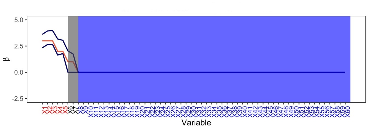
(a) Sparsified simultaneous confidence intervals.

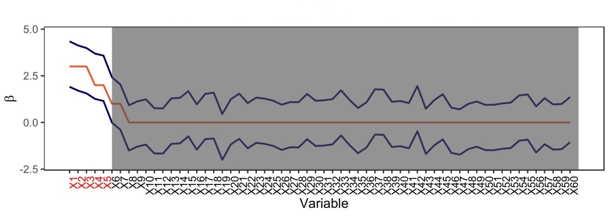
(b) Simultaneous confidence intervals by debiased Lasso.

Figure 1: Graphical comparison of our method and Zhang and Cheng, (2017)’s method.

This article contributes to the literature in the following aspects. We integrate the sparsity feature into the simultaneous confidence intervals to provide insights on model selection uncertainty besides carrying out inference for regression coefficients. Under a consistent model selection procedure, we have established the asymptotic coverage probability. We develop a graphical representation of the proposed method to enhance the visualization for both parameter and model uncertainty. In addition to satisfactory performance in typical settings, we numerically show that the proposed simultaneous confidence intervals perform well in the weak signal settings compared to the existing methods.

The article is organized as follows. In Section 2, we introduce our sparsified simultaneous confidence intervals, establish its theoretical properties, develop its graphical presentation, and discuss its connections to other methods. We explain the key ingredient in our approach, selection by partitioning solution paths, in Section 3. Numerical experiments and real data examples evidence the advantages of our approach in Sections 4 and 5. We conclude in Section 6 and relegate proofs to the supplementary materials.

2 Inference for High-Dimensional Linear Models

Throughout the article, we focus on the inference tasks for the linear model $\mathbf{y}=\mathbf{X}\boldsymbol{\beta}^{0}+\boldsymbol{\varepsilon}$ where $\boldsymbol{\varepsilon}\sim N(\mathbf{0},\sigma^{2}\mathbf{I}_{n})$, $\mathbf{y}\in\mathbb{R}^{n}$ is the response vector, and $\mathbf{X}\in\mathbb{R}^{n\times p}$ is the fixed design matrix containing $p$ covariates. The parameter vector $\boldsymbol{\beta}^{0}=(\beta^{0}_{1},\cdots,\beta^{0}_{p})^{T}\in\mathbb{R}^{p}$ is assumed to be sparse with a small number of nonzero coefficients. We denote the index sets of the nonzero and zero coefficients as $\mathcal{S}_{0}=\{j:\beta^{0}_{j}\neq 0\}$ and $\mathcal{S}_{0}^{c}=\{j:\beta^{0}_{j}=0\}$, respectively. We denote the cardinality of the active set as $s_{0}=|\mathcal{S}_{0}|$ and assume it is smaller than $p$, and the dimension $p$ can be larger than $n$.

2.1 Sparsified Simultaneous Confidence Intervals

We propose a new type of simultaneous confidence intervals, namely sparsified simultaneous confidence intervals (SSCI). It consists a sequence of confidence intervals that contains all the true coefficients simultaneously with a confidence level $1-\alpha$. That is, let $\text{SSCI}_{1-\alpha}=\{\boldsymbol{\beta}\in\mathbb{R}^{p}:\underline{{\beta}}_{j}\leq\beta_{j}\leq\overline{{\beta}}_{j},j=1,\dots,p\}$ where $\underline{{\beta}}_{j}$ and $\overline{{\beta}}_{j}$ are the lower and upper bounds of $j$-th coefficient, such that $\mathbf{P}(\boldsymbol{\beta}^{0}\in\text{SSCI}_{1-\alpha})=1-\alpha$. The proposed SSCI is sparse in the sense that some of its intervals’ upper and/or lower bounds are shrunken to zero, signaling the significance of the corresponding coefficients.

To construct SSCI, we bootstrap a two-stage estimator that contains both the consistent model selection procedure and the refitted estimation procedure. Given an observed sample, we first apply the two-stage estimator to select an initial model and obtain the refitted coefficient estimate. We further generate bootstrap samples using the refitted estimate via the celebrated residual bootstrap (Freedman, , 1981; Efron, , 1992). For each bootstrap sample, we apply the same two-stage estimator to identify the bootstrap model $\hat{\mathcal{S}}^{(b)}$ and obtain the refitted bootstrap coefficient estimate $\hat{\boldsymbol{\beta}}^{(b)}$. After removing the $\alpha$ proportion of bootstrap estimates according to their outlyingness, we use the remaining bootstrap estimates to construct SSCI. The details of this procedure are outlined in Algorithm 1.

Algorithm 1 Sparsified simultaneous confidence intervals

• $\mathbf{y}$, $\mathbf{X}$;

• Sparsified simultaneous confidence intervals at the confidence level of $1-\alpha$;

• Apply a two-stage estimation procedure on $\left\{\mathbf{y},\mathbf{X}\right\}$ to obtain the selected model $\tilde{\mathcal{S}}_{0}$ and its refitted coefficient estimate $\tilde{\boldsymbol{\beta}}$;

• Generate bootstrap samples $\left\{(\mathbf{y}^{(b)},\mathbf{X})\right\}^{B}_{b=1}$ via residual bootstrap with $\tilde{\boldsymbol{\beta}}$;

• For $b=1,\dots,B,$ apply the same two-stage estimation procedure on $(\mathbf{y}^{(b)},\mathbf{X})$ to obtain bootstrap model $\hat{\mathcal{S}}^{(b)}$ and its refitted bootstrap estimate $\hat{\boldsymbol{\beta}}^{(b)}$;

• Compute the outlyingness score $O^{(b)}=\max_{j\in\{1,\dots,p\}}\big{|}(\hat{\beta}^{(b)}_{j}-\bar{\hat{\beta}}_{j})/\widehat{\text{SE}}(\hat{\beta}_{j})\big{|},b=1,...,B$;

• Construct the $\text{SSCI}_{1-\alpha}$ by letting $\underline{{\beta}}_{j}=\min_{b\in\mathcal{B}_{1-\alpha}}\hat{\beta}^{(b)}_{j}$ and $\overline{{\beta}}_{j}=\max_{b\in\mathcal{B}_{1-\alpha}}\hat{\beta}^{(b)}_{j}$
      for $j=1,...,p$, where $\mathcal{B}_{1-\alpha}=\{b:O^{(b)}\leq q_{1-\alpha}\}$ and $q_{1-\alpha}$ is $(1-\alpha)$-quantile of $\{O^{(b)}\}_{b=1}^{B}$.

For each bootstrap estimate, we measure its outlyingness relative to other bootstrap estimates, i.e., outlyingness score, by calculating the maximum absolute value of standardized coefficients $O^{(b)}=O(\hat{\boldsymbol{\beta}}^{(b)})=\max_{j\in\{1,\dots,p\}}\big{|}(\hat{\beta}^{(b)}_{j}-\bar{\hat{\beta}}_{j})/\widehat{\text{SE}}(\hat{\beta}_{j})\big{|}$, where $\bar{\hat{\beta}}_{j}=\sum^{B}_{b=1}\hat{\beta}^{(b)}_{j}/B$ and $\widehat{\text{SE}}(\hat{\beta}_{j})=\big{(}\sum^{B}_{b=1}\big{(}\hat{\beta}^{(b)}_{j}-\bar{\hat{\beta}}_{j}\big{)}^{2}/(B-1)\big{)}^{1/2}$ is the bootstrap standard error estimate. Intuitively, standardized coefficients reveal the variability of each bootstrap coefficient estimates, while the maximum absolute value among all covariates measures the overall outlyingness of the bootstrap estimate and the bootstrap model. Hence, the outlyingness scores identify the extreme and rare bootstrap models and estimates. For example, in one bootstrap iteration, if a two-stage estimator selects a particular covariate that has never been selected in other bootstrap iterations, the outlyingness score of this coefficient may be very large, which implies that this bootstrap estimate may be unusual and should be discarded. In Step 5 of Algorithm 1, we remove these outlying bootstrap estimates by cutting the outlying scores at its $(1-\alpha)$-percentile, and use the remaining bootstrap estimates to construct our intervals.

Since the bootstrap estimates are likely sparse, the boundaries of the confidence intervals of SSCI are likely sparse too, which carry important information about the covariates and the model. In particular, we define three groups of covariates: significant covariates whose intervals do not contain zero, denoted as $\hat{\mathcal{S}}_{\text{1}}=\{j:\underline{{\beta}}_{j}\cdot\overline{{\beta}}_{j}>0\}$; plausible covariates whose intervals contain zero but has non-zero width, denoted as $\hat{\mathcal{S}}_{\text{2}}=\{j:\underline{{\beta}}_{j}\cdot\overline{{\beta}}_{j}\leq 0\text{ and }\underline{{\beta}}_{j}\neq\overline{{\beta}}_{j}\}$, and unimportant covariates whose intervals contain zero and have zero-width, denoted as $\hat{\mathcal{S}}_{\text{3}}=\{j:\underline{{\beta}}_{j}=\overline{{\beta}}_{j}=0\}$. The significant covariates are the ones strongly associated with the response variable and should be included in the final model at $1-\alpha$ confidence level. The plausible covariates are the ones weakly associated with the response. We do not have enough evidence to prove their significance nor to disqualify them for the final model. The unimportant covariates are the superfluous predictors that should be excluded from the final model at $1-\alpha$ confidence level. Therefore, not only do we have the estimation uncertainties for each coefficient estimate, but we also obtain model information based on the sparsity feature of the intervals.

The proposed algorithm can be coupled with many two-stage estimators that consists of a consistent model selection procedure followed by a consistent refitted regression estimator. For model selection methods, we study Lasso, adaptive Lasso, and Liu and Wang, (2018)’s SPSP based on the solution path of adaptive Lasso (SPSP+AdaLasso) or Lasso (SPSP+Lasso). For the refitted estimator $\tilde{\boldsymbol{\beta}}$, we adopt the least square refitted estimator through out this article, that is, $\tilde{\boldsymbol{\beta}}_{\tilde{S}}=(\mathbf{X}_{\tilde{S}}^{T}\mathbf{X}_{\tilde{S}})^{-1}\mathbf{X}_{\tilde{S}}^{T}\mathbf{Y}\in\mathbb{R}^{|\tilde{S}|}$ and $\tilde{\boldsymbol{\beta}}_{\tilde{S}^{c}}=\mathbf{0}\in\mathbb{R}^{p-|\tilde{S}|}$. Through numerical studies, among all the methods we compared, we find SPSP is the best model selector for constructing the proposed intervals in terms of stability and coverage probability. Using SPSP, our intervals are noticeably narrower than other classical simultaneous confidence intervals, at the same time offering more accurate information about the true coefficient vector and the true model. Therefore, we recommend Liu and Wang, (2018)’s method as the default selection method for our proposed approach.

Lastly, the proposed method allows alternative outlyingness scores to be implemented. By defining outlyingness scores differently, we are able to construct different inference tools such as individual confidence intervals, simultaneous confidence intervals, or model confidence set (Ferrari and Yang, , 2015). We leave this topic for future work.

2.2 Theoretical Properties

In this section, we establish the theoretical properties of the proposed method, such as the coverage probability of the SSCI under various model selection methods. Without loss of generality, we assume $\mathbf{X}$ are standardized with zero mean and unit variance. Let $\mathbf{X}_{\mathcal{S}_{0}}\in\mathbb{R}^{n\times s_{0}}$ be the true signal covariates matrix and $s_{0}=|\mathcal{S}_{0}|$.

Theorem 1

Suppose the selection method selects the true model with the probability $1-2e^{-h(n)}$, that is $\mathbf{P}(\tilde{\mathcal{S}}=\mathcal{S}_{0})=1-2e^{-h(n)}$. Then, with $B=o(e^{h(n)})$, for any confidence level of $\alpha\in(0,1)$, the $\textup{SSCI}_{1-\alpha}$ constructed in Algorithm 1 has the asymptotic coverage probability $\mathbf{P}(\boldsymbol{\beta}^{0}\in\textup{SSCI}_{1-\alpha})\xrightarrow{n\rightarrow\infty}1-\alpha.$

Remark 1. Theorem 1 implies that, with a consistent selection procedure, the proposed SSCI can asymptotically achieve the nominal coverage probability. The function $h(n)$ has different forms when different selection method is adopted. We have $h(n)=n^{c}$ with $0\leq c<1$ for Lasso, and $h(n)=\gamma n$ for Adaptive Lasso and SPSP. We further discuss the induced properties from Theorem 1 when we incorporate Lasso, adaptive Lasso, and SPSP in our approach as shown in Corollaries 1.1, 1.2 and 1.3.

Corollary 1.1 (Lasso)

Let $\tilde{\mathcal{S}}^{\textup{Lasso}}(\lambda_{n})$ be the model selected by the Lasso with the tuning parameter $\lambda_{n}$ and $\textup{SSCI}^{\textup{Lasso}}_{1-\alpha}(\lambda_{n})$ be constructed by Algorithm 1 using the Lasso with the tuning parameter $\lambda_{n}$ and the least square refitted estimate. Under the strong irrepresentable condition (Zhao and Yu, , 2006), $\mathbf{P}(\tilde{\mathcal{S}}^{\textup{Lasso}}(\lambda_{n})=\mathcal{S}_{0})\geq 1-2e^{-n^{c}}$ if $\lambda_{n}/n\rightarrow 0$ and $\lambda_{n}/n^{(1+c)/2}\rightarrow\infty$ with $0\leq c<1$, and $B=o(e^{n^{c}})$ , we have $\mathbf{P}(\boldsymbol{\beta}^{0}\in\textup{SSCI}^{\textup{Lasso}}_{1-\alpha}(\lambda_{n}))\xrightarrow{n\rightarrow\infty}1-\alpha.$

Corollary 1.2 (Adaptive Lasso)

Let $\tilde{\mathcal{S}}^{\textup{Ada}}(\lambda_{n})$ be the model selected by the adaptive Lasso with the tuning parameter $\lambda_{n}$ and $\textup{SSCI}^{\textup{Ada}}_{1-\alpha}(\lambda_{n})$ be constructed by Algorithm 1 using the adaptive Lasso with the tuning parameter $\lambda_{n}$ and the least square refitted estimate. Under the restricted eigenvalue condition (van de Geer et al., , 2011), $\mathbf{P}(\tilde{\mathcal{S}}^{\textup{Ada}}(\lambda_{n})=\mathcal{S}_{0})\geq 1-2e^{-\gamma n}$ if $\lambda_{n}=4\sigma\sqrt{2\gamma+2\log p/n}$ and $\gamma\rightarrow 0$. Further if $B=o(e^{\gamma n})$, we have $\mathbf{P}(\boldsymbol{\beta}^{0}\in\textup{SSCI}^{\textup{Ada}}_{1-\alpha}(\lambda_{n}))\xrightarrow{n\rightarrow\infty}1-\alpha.$

Corollary 1.3 (SPSP)

Let $\tilde{\mathcal{S}}^{\textup{SPSP}}$ be the model selected by SPSP and $\textup{SSCI}^{\textup{SPSP}}_{1-\alpha}$ be constructed by Algorithm 1 using the SPSP and the least square refitted estimate. Under the compatibility condition in Bühlmann and van de Geer, (2011), and the weak identifiability condition in Liu and Wang, (2018), the SPSP can select the true model $\mathcal{S}_{0}$ over $\lambda\in[4\sigma\sqrt{4\gamma+{2\log p}/{n}},+\infty]$ with probability at least $1-2e^{-\gamma n}$, that is $\mathbf{P}(\tilde{\mathcal{S}}^{\textup{SPSP}}=\mathcal{S}_{0})\geq(1-2e^{-\gamma n})$. Further if $B=o(e^{\gamma n})$, we have $\mathbf{P}(\boldsymbol{\beta}^{0}\in\textup{SSCI}^{\textup{SPSP}}_{1-\alpha})\xrightarrow{n\rightarrow\infty}1-\alpha.$

2.3 Visualization and Comparison with Other Methods

In this section, we develop an intuitive graphical tool, namely the SSCI plot, to visualize the estimation uncertainty. Specifically, we plot the confidence intervals of all covariates side by side but rearrange them in the following order: We place the significant covariates with all positive (or all negative) interval boundaries on the left (or right) end of the horizontal axis. The plausible and unimportant covariates are placed in the middle with grey and blue shades. The bootstrap estimates contained in SSCI are drawn in a light blue line while the true coefficient (if known) is in red.

We present a simple example using the simulated data from Example 4 in Section 4. We construct SSCI using SPSP+AdaLasso, SPSP+Lasso, AdaLasso, and Lasso and visualize them in Figure 2. For the sake of simplicity, we only display the total number of covariates instead of the variables’ names.

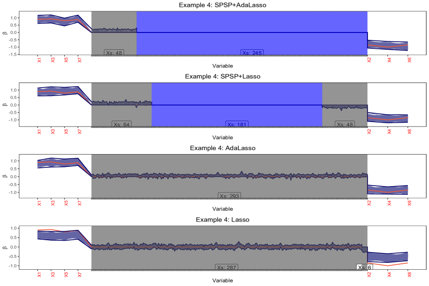
Figure 2: Graphical presentation of SSCI.

In the figure, the estimation uncertainty can be reflected by the vertical widths of the intervals. The significant covariates are labeled in red to highlight their importance in the model. For the plausible covariates, their confidence intervals contain zero; hence we put these covariates on the “waiting list”. The confidence intervals of unimportant covariates all shrunk to zero, implying they should be excluded from the model.

It is worth noting that the SSCIs by SPSP perform better than the others in this example. For instance, the plausible covariates of SSCI by SPSP are much fewer than the rest, indicating the stability of SPSP. This is because the bootstrap models of AdaLasso and Lasso fail to reach any consensus. In addition, the vertical widths of SSCIs by SPSP are, on average narrower than the other SSCIs, indicating a lower estimation uncertainty. We summarize their vertical widths in Table 1.

Table 1: Comparison of the widths of SSCI by different selection methods

	Selection Method
Width of SSCI	SPSP+AdaLasso	SPSP+Lasso	AdaLasso	Lasso
Average width of all covariates	0.048	0.086	0.183	0.226
Average width of signals	0.539	0.537	0.512	0.464
Average width of non-signals	0.036	0.076	0.175	0.220

Lastly, we graphically compare SSCI with the simultaneous confidence region (SCR) and the simultaneous confidence intervals based on debiased Lasso (SCI debiased Lasso), all of which capture the true coefficients at the $1-\alpha$ confidence level.

The SCR (Chatterjee and Lahiri, , 2011) is defined as $\text{SCR}_{1-\alpha}=\{\boldsymbol{\beta}\in\mathbb{R}^{p}:\lVert\boldsymbol{\beta}-\hat{\boldsymbol{\beta}}\lVert\leq n^{-1/2}\hat{t}_{1-\alpha}\}$, where $\hat{\boldsymbol{\beta}}$ is the Lasso estimate, $\lVert\cdot\lVert$ is $\ell_{2}$ norm, and $\hat{t}_{1-\alpha}$ is the $1-\alpha$ quantile of the $\ell_{2}$ norms of the centered and scaled bootstrap estimates. Therefore, the shape of SCR is an ellipsoid centered at $\hat{\boldsymbol{\beta}}$ capturing $1-\alpha$ proportion of the bootstrap estimates, as shown in Figure 3a. The data is simulated with $n=200$, $p=3$, $(\beta_{1},\beta_{2},\beta_{3})=(3,2,0)$, $\sigma_{\varepsilon}=3.5$.

The SCI debiased Lasso (Zhang and Cheng, , 2017) is defined as $\text{SCI}^{\textup{deb}}_{1-\alpha}=\{\boldsymbol{\beta}\in\mathbb{R}^{p}:\sqrt{n}|\boldsymbol{\beta}-\hat{\boldsymbol{\beta}}^{\textup{deb}}|\leq c^{*}_{1-\alpha}\mathbf{1}\}$ where $\hat{\boldsymbol{\beta}}^{\textup{deb}}$ is the debiased Lasso estimate, and $c^{*}_{1-\alpha}$ is $1-\alpha$ bootstrap critical value in Zhang and Cheng, (2017), and $\mathbf{1}=(1,...,1)^{T}$. Therefore, the shape of SCI debiased Lasso is a hypercube centered at $\hat{\boldsymbol{\beta}}^{\textup{deb}}$, as shown in Figure 3b, using the same data.

In contrast, our SSCI is a special type of hyperrectangle in $\mathbb{R}^{p}$ with some of its edges shrunken to zero, representing the unimportant covariates. An example is shown in Figures 3c and 3d using the same data. The bootstrapped SPSP estimates are shown in dots. The SSCI is the black hyperrectangle with its third dimension, $\beta_{3}$, shrunken to zero.

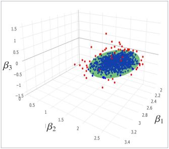
(a) SCR

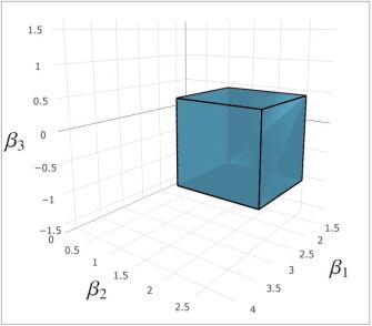
(b) SCI

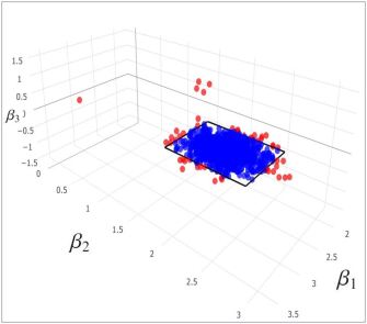
(c) SSCI

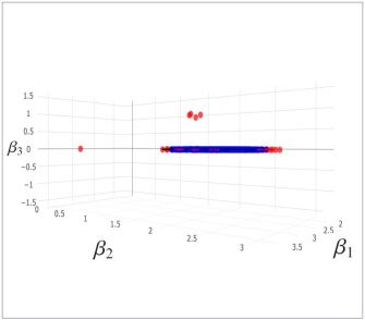
(d) SSCI, 2nd view

Figure 3: Graphical comparison of SCR, SCI debiased Lasso, and SSCI. Note that Panels (c) and (d) shows the same SSCI from different perspectives.

Even though all three types of confidence sets claim to capture the true coefficients at the $1-\alpha$ confidence level, they are quite different in terms of usage. SCR often offers the tightest confidence set than SCI debiased Lasso since the ellipsoid is able to capture more bootstrap estimates than the hypercube of the same volume. SCI debiased Lasso is easy to interpret since it consists of $p$ individual intervals, whereas SCR cannot be expressed in the same fashion since the interval boundary for one coefficient depends on the rest of the coefficients. Unfortunately, neither case can offer us model information. On the other hand, SSCI is often one of the tightest due to the stability of SPSP, and it comes with easy interpretability. The shrunken edges of SSCI indicate the exclusion of the corresponding covariates in the final model. Such a message is not available in neither SCR nor SCI debiased Lasso.

2.4 Model Insights

Since the refitted parameter estimate $\tilde{\boldsymbol{\beta}}$ is obtained after the model $\tilde{\mathcal{S}}$ is selected, the overall estimation uncertainty of $\tilde{\boldsymbol{\beta}}$, measured by SSCI, can be decomposed as $\textup{Var}(\tilde{\boldsymbol{\beta}})=\mathbb{E}(\textup{Var}(\tilde{\boldsymbol{\beta}}|\tilde{\mathcal{S}}))+\textup{Var}(\mathbb{E}(\tilde{\boldsymbol{\beta}}|\tilde{\mathcal{S}}))$. We refer to the first term on the right as the parameter uncertainty, representing the averaged parameter estimation uncertainty conditional on selected models. We refer to the second term as the model uncertainty, which represents the extra parameter estimation uncertainty owing to model selection.

With the consistent model selector and least square estimator, the parameter uncertainty converges to 0 at the order $1/n$. Since the probability of selecting the true model is typical $1-2\exp(-Cn)$, the model uncertainty converges to 0 much faster. Hence, asymptotically, the overall estimation uncertainty is mostly the parameter uncertainty. On the other hand, under the finite sample size, both the model uncertainty and parameter uncertainty are non-negligible. In this case, we can still utilize SSCI to provide insights about models, admitting that the asymptotic results are not directly applicable and the finite sample theoretical results are hard to derive.

Based on the graphical tools introduced previously, we can visualize the parameter uncertainty as well as the model uncertainty. Using the simulated data under the setting in Section 1, we first generate the SSCI plot in Figure 4. There are, in total, three unique bootstrap models for this data set, so we plot the simultaneous confidence intervals based on each bootstrap model in the shade in the first three panels of Figure 4 and overlay them in the last panel. We can see that the simultaneous confidence intervals based on each bootstrap model are narrower than SSCI. The difference represents the increased estimation uncertainty from conditional on one selected model to marginalizing over all selected models. Meanwhile, the estimation uncertainty is the most inflated for the coefficients of $X_{6}$ and $X_{7}$ because these covariates are selected differently in the bootstrap models.

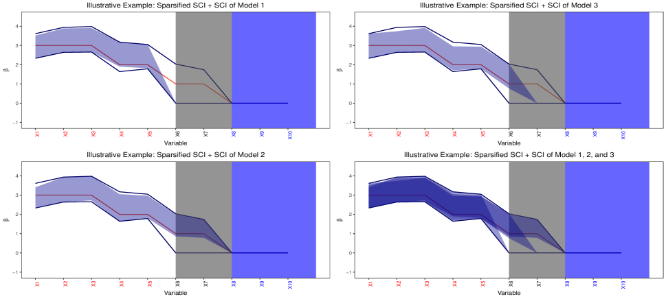
Figure 4: Illustration of the SSCI and the SCIs of three bootstrap models.

Under the finite sample size, SSCI naturally defines two nested models: 1) the lower bound model with the significant covariates, denoted as $\underline{\mathcal{S}}=\hat{\mathcal{S}}_{1}$; 2) the upper bound model with the significant and plausible covariates, denoted as $\overline{\mathcal{S}}=\hat{\mathcal{S}}_{1}\cup\hat{\mathcal{S}}_{2}$. It is straightforward to show that the two models trap the true model $\mathcal{S}_{0}$ with at least the same confidence level. We call this pair of models model confidence bounds (MCB) induced by SSCI. Conceptually, our MCB extends the idea of the classical confidence interval for a population parameter to the case of model selection. The lower bound model is regarded as the most parsimonious model that cannot afford to lose one more covariate. In contrast, the upper bound model is viewed as the most complex model that cannot tolerate one extra covariate.

We can define the width of MCB as $w=|\overline{\mathcal{S}}\setminus\underline{\mathcal{S}}|=|\hat{\mathcal{S}}_{2}|$, i.e., the number of plausible covariates. Similar to the width of the classical confidence interval, the MCB width can be potentially used as a measure of model selection stability. Since MCB can be coupled with various selection methods, we can compare their MCB widths at the same confidence level.

As an example, we construct the MCBs using SPSP+AdaLasso, SPSP+Lasso, AdaLasso, and Lasso at different confidence levels using the simulated data from Example 4 in Section 4. Figure 5 shows how these MCBs behave as the confidence level changes. The horizontal axis represents the covariate, whereas the vertical axis represents the confidence level. At each confidence level, the lower bound model (or the significant covariates) is the red area. The plausible covariates are the grey areas, which are also the MCB width. The upper bound model consists of both red and grey areas. The unimportant covariates are the blue area.

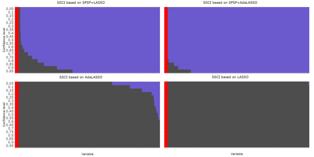
Figure 5: MCB induced by SSCI at various confidence levels by different selection methods.

As we can see, the MCB width increases as the confidence level increases, which is consistent with the traditional confidence intervals. Among these MCBs, the MCBs by SPSP are able to maintain small widths throughout the confidence levels, whereas the MCBs by AdaLasso and Lasso all have large widths. This evidence implies that the SPSP-based method selects the model more stably and results in fewer unique bootstrap models than Lasso and AdaLasso. More discussion of the SPSP method can be found in Section 3.

3 Selection by Partitioning Solution Paths

Our SSCI can be equipped with different variable selection and estimation methods. A more accurate and stable method will help to construct narrower intervals as well as more zero-width intervals and provide an informative MCB. Throughout this article, we rely on SPSP (Liu and Wang, , 2018) due to its stability and accuracy.

The idea of SPSP is to partition the covariates into “relevant” and “irrelevant” sets by utilizing the entire solution paths. It mainly has three advantages. First, SPSP is more stable and accurate (low false positive and false negative rates) than other variable selection approaches. As a result, it will generate fewer unique models among bootstrap samples. Second, SPSP is computationally more efficient because it does not need to calculate the solutions multiple times for all tuning parameters when cross-validation is involved. When the bootstrap technique is applied, this advantage may dramatically decrease the computing time. Third, one can flexibly incorporate SPSP with the solution paths of Lasso, adaptive Lasso, and other penalized estimators.

Here, we briefly introduce the SPSP approach. More in-depth discussion can be found in Liu and Wang, (2018). Given a tuning parameter $\lambda_{k}$ and the corresponding coefficients estimation $\hat{\beta}_{1},\dots,\hat{\beta}_{p}$, it orders the coefficients estimation as $\hat{\beta}_{(1)},\dots,\hat{\beta}_{(p)}$. Based on the order statistics, it defines the gap between a relevant set ($\hat{\mathcal{S}}_{k}$) and an irrelevant set ($\hat{\mathcal{S}}^{c}_{k}$) as the adjacent distance between two order statistics, $\hat{\beta}_{(p-\hat{s}_{k})}$ and $\hat{\beta}_{(p-\hat{s}_{k}+1)}$. This gap (adjacent distance) is denoted as $D(\hat{\mathcal{S}}_{k},\hat{\mathcal{S}}^{c}_{k})=D^{(k)}_{p-\hat{s}_{k}+1}=\hat{\beta}^{(k)}_{(p-\hat{s}_{k}+1)}-\hat{\beta}^{(k)}_{(p-\hat{s}_{k})}$. With this notation, the largest adjacent distance in $\hat{\mathcal{S}}_{k}$ can be defined as $D_{\text{max}}(\hat{\mathcal{S}}_{k})=\text{max}\{D^{(k)}_{j}:j>p-\hat{s}_{k}+1\}$. Likewise, $D_{\text{max}}(\hat{\mathcal{S}}^{c}_{k})=\text{max}\{D^{(k)}_{j}:j<p-\hat{s}_{k}+1\}$ is the largest adjacent distance in $\hat{\mathcal{S}}^{c}_{k}$. Then the final step of the SPSP can be implemented by finding these two sets such that the gap is greater than the largest adjacent distance in irrelevant set ($\hat{\mathcal{S}}_{k}$), and smaller than the largest adjacent distance in the relevant set ($\hat{\mathcal{S}}^{c}_{k}$). The SPSP adaptively finds a large enough distance, $D(\hat{\mathcal{S}}_{k},\hat{\mathcal{S}}^{c}_{k})$, which satisfies $\frac{D_{\text{max}}(\hat{\mathcal{S}}_{k})}{D(\hat{\mathcal{S}}_{k},\hat{\mathcal{S}}^{c}_{k})}\leq R<\frac{D(\hat{\mathcal{S}}_{k},\hat{\mathcal{S}}^{c}_{k})}{D_{\text{max}}(\hat{\mathcal{S}}^{c}_{k})},$ where the constant control value $R$ can be estimated from the data. Finally, the SPSP method identifies a set of relevant variables $\tilde{\mathcal{S}}^{\text{SPSP}}$ as the union of all $\hat{\mathcal{S}}_{k}$ for the tuning parameters $\lambda_{1}<\lambda_{2}<\cdots<\lambda_{k}$, i.e $\tilde{\mathcal{S}}^{\text{SPSP}}=\cup^{K}_{k=1}\hat{\mathcal{S}}_{k},$ as the estimate of the true model $\mathcal{S}_{0}$. Afterwards, we refit the model to obtain the least square estimation $\hat{\boldsymbol{\beta}}^{\text{LS}}_{\tilde{\mathcal{S}}^{\text{SPSP}}}$ for the selected covariates $\tilde{\mathcal{S}}^{\text{SPSP}}$ but keep zero coefficients for unselected covariates. The estimation of coefficients for SPSP are $\hat{\boldsymbol{\beta}}^{\text{SPSP}}=(\hat{\boldsymbol{\beta}}^{\text{LS}}_{\tilde{\mathcal{S}}^{\text{SPSP}}},\boldsymbol{0}_{\hat{\mathcal{S}}^{c}}).$

4 Simulation Studies

We investigate the performance of our SSCI in the high-dimensional settings with independent or correlated covariates and low-dimensional settings with weak signals. Under each setting, we construct SSCIs using four variable selection methods: SPSP based on the solution paths of adaptive Lasso (SPSP+AdaLasso) and Lasso (SPSP+Lasso), adaptive Lasso with 10-fold cross-validation (AdaLasso+CV), and Lasso with 10-fold cross-validation (Lasso+CV). We also construct SCI debiased Lasso. Lastly, we construct the simultaneous confidence intervals using the OLS estimates under the true model as a benchmark for estimation uncertainty (denoted as “Oracle”). We set the confidence level as 95%. To obtain these results, we develop SSCI package to construct and visualize the SSCI based on the glmnet and ggplot2 packages (Hastie and Qian, , 2014; Wickham, , 2011). Below is a list of settings.

Study 1: We generate 200 data sets from the linear model with $\mathbf{X}_{j}\sim N(0,1),\varepsilon_{i}\sim N(0,1)$, for $i=1,\dots,n$ and $j=1,\dots,p$, and set $B=1000$.

• (Independent covariates) Let $n=200$, $p=300$, and $\boldsymbol{\beta}^{0}=(4,3.5,3,2.5,2,0,...,0)$.

• (Correlated covariates) Let $n=50$, $p=100$, and $\boldsymbol{\beta}^{0}=(3,2,1.5,0,...,0)$. The pairwise covariate correlation is $\text{cor}(\mathbf{X}_{j},\mathbf{X}_{j^{\prime}})=0.5^{|j-{j^{\prime}}|}$.

• The setting is same as the Example 2 except the $n=200$ and $p=300$.

• (Correlated covariates with coefficients of alternating signs) Let $n=200$, $p=300$, $\boldsymbol{\beta}^{0}=(0.9,-0.85,0.93,-1,0.8,-0.85,0.88,0,...,0)$, $\text{cor}(\mathbf{X}_{j},\mathbf{X}_{j^{\prime}})=0.5^{|j-{j^{\prime}}|}$.

Table 2: Simulation results of Examples 1 through 7

Study 1: High-dimensional settings
		Simultaneous Confidence Intervals			Model Confidence Bounds
Setting	Method	$\text{P}^{\text{SCI}}_{\text{coverage}}(\%)$	$\bar{w}_{\mathcal{S}_{0}}$	$\bar{w}_{\mathcal{S}_{0}^{c}}$	$\text{P}^{\text{MCB}}_{\text{coverage}}(\%)$	$\bar{w}$
	SSCI (SPSP+AdaLasso)	94.50	0.35 (0.00)	0.00 (0.00)	100.00	0.00
	SSCI (SPSP+Lasso)	95.00	0.35 (0.00)	0.00 (0.00)	100.00	100.00
Example 1	SSCI (AdaLasso+CV)	95.50	0.35 (0.00)	0.00 (0.00)	100.00	0.00
$s$=5, $\rho$=0	SSCI (Lasso+CV)	76.00	0.45 (0.00)	0.36 (0.00)	86.50	294.78
$n$=200, $p$=300	SCI (Debiased Lasso)	97.50	0.63 (0.00)	0.63 (0.00)	—	—
	Oracle	93.50	0.35 (0.00)	0.00 (0.00)	—	—
	SSCI (SPSP+AdaLasso)	94.00	1.35 (0.06)	0.06 (0.02)	94.50	6.58
	SSCI (SPSP+Lasso)	93.00	1.09 (0.03)	0.00 (0.00)	99.00	99.00
Example 2	SSCI (AdaLasso+CV)	95.00	0.96 (0.01)	0.15 (0.01)	100.00	38.38
$s$=3, $\rho$=0.5	SSCI (Lasso+CV)	76.00	1.02 (0.02)	0.48 (0.02)	83.50	93.40
$n$=50, $p$=100	SCI (Debiased Lasso)	94.50	1.25 (0.01)	1.25 (0.01)	—	—
	Oracle	91.50	0.81 (0.01)	0.00 (0.00)	—	—
	SSCI (SPSP+AdaLasso)	97.50	0.66 (0.04)	0.00 (0.00)	100.00	0.32
	SSCI (SPSP+Lasso)	94.50	0.40 (0.00)	0.00 (0.00)	100.00	100.00
Example 3	SSCI (AdaLasso+CV)	95.00	0.39 (0.00)	0.00 (0.00)	100.00	0.00
$s$=3, $\rho$=0.5	SSCI (Lasso+CV)	97.50	0.58 (0.01)	0.39 (0.00)	98.50	296.99
$n$=200, $p$=300	SCI (Debiased Lasso)	94.50	0.61 (0.00)	0.61 (0.00)	—	—
	Oracle	96.00	0.39 (0.00)	0.00 (0.00)	—	—
	SSCI (SPSP+AdaLasso)	96.50	0.60 (0.01)	0.04 (0.00)	100.00	57.09
	SSCI (SPSP+Lasso)	96.50	0.92 (0.02)	0.19 (0.01)	100.00	100.00
Example 4	SSCI (AdaLasso+CV)	90.00	0.61 (0.01)	0.37 (0.00)	98.50	293.21
$s$=7, $\rho$=0.5	SSCI (Lasso+CV)	30.00	0.57 (0.01)	0.40 (0.00)	77.00	292.50
$n$=200, $p$=300	SCI (Debiased Lasso)	98.00	0.97 (0.00)	0.97 (0.00)	—	—
	Oracle	99.50	0.45 (0.00)	0.00 (0.00)	—	—
Study 2: Weak signal settings
		Simultaneous Confidence Intervals			Model Confidence Bounds		Weak Signal
Setting	Method	$\text{P}^{\text{SCI}}_{\text{coverage}}(\%)$	$\bar{w}_{\mathcal{S}_{0}}$	$\bar{w}_{\mathcal{S}_{0}^{c}}$	$\text{P}^{\text{MCB}}_{\text{coverage}}(\%)$	$\bar{w}$	$\text{P}^{\theta}_{\text{coverage}}(\%)$
	SSCI (SPSP+AdaLasso)	91.00	1.24 (0.02)	0.85 (0.02)	100.00	19.53	99.75
	SSCI (SPSP+Lasso)	78.50	1.22 (0.02)	0.80 (0.02)	99.75	19.45	97.50
Example 5	SSCI (AdaLasso+CV)	89.25	1.11 (0.02)	0.75 (0.02)	100.00	18.89	100.00
$\rho$=0	SSCI (Lasso+CV)	64.00	0.99 (0.02)	0.68 (0.01)	100.00	19.40	99.00
	SCI (Debiased Lasso)	96.25	1.37 (0.01)	1.37 (0.01)	—	—	99.50
	Oracle	90.50	0.96 (0.00)	0.00 (0.00)	—	—	98.00
	SSCI (SPSP+AdaLasso)	94.75	1.31 (0.02)	0.87 (0.02)	100.00	19.59	100.00
	SSCI (SPSP+Lasso)	84.50	1.30 (0.03)	0.78 (0.02)	99.75	19.23	98.25
Example 6	SSCI (AdaLasso+CV)	93.25	1.15 (0.02)	0.75 (0.02)	100.00	18.79	100.00
$\rho$=0.2	SSCI (Lasso+CV)	78.00	1.03 (0.01)	0.68 (0.01)	99.75	18.96	100.00
	SCI (Debiased Lasso)	94.50	1.42 (0.00)	1.42 (0.01)	—	—	100.00
	Oracle	92.00	0.99 (0.00)	0.00 (0.00)	—	—	98.00
	SSCI (SPSP+AdaLasso)	92.50	1.63 (0.03)	1.05 (0.02)	100.00	19.77	100.00
	SSCI (SPSP+Lasso)	95.00	1.59 (0.03)	0.92 (0.02)	100.00	19.35	100.00
Example 7	SSCI (AdaLasso+CV)	97.25	1.40 (0.02)	0.82 (0.02)	100.00	19.13	100.00
$\rho$=0.5	SSCI (Lasso+CV)	93.25	1.23 (0.02)	0.74 (0.01)	100.00	18.98	100.00
	SCI (Debiased Lasso)	96.50	1.75 (0.01)	1.75 (0.01)	—	—	99.75
	Oracle	91.00	1.18 (0.01)	0.00 (0.00)	—	—	97.00
Note: SSCI is sparsified simultaneous confidence intervals. “Oracle” is simultaneous confidence intervals using the OLS
estimates under the true model. We compare the SSCI using five variable selection methods: solution paths of adaptive Lasso
(SPSP+AdaLasso) and Lasso (SPSP+Lasso), adaptive Lasso with 10-fold cross-validation (AdaLasso+CV), Lasso with 10-fold
cross-validation (Lasso+CV), and simultaneous confidence intervals based on debiased Lasso method.

We compare different methods in the following aspects: coverage probability of the simultaneous confidence intervals $\text{P}^{\text{SCI}}_{\text{coverage}}$, average interval width of true signals $\bar{w}_{\mathcal{S}_{0}}$ and non-signals $\bar{w}_{\mathcal{S}_{0}^{c}}$, MCB coverage probability $\text{P}^{\text{MCB}}_{\text{coverage}}$, average MCB width $\bar{w}$, and the coverage rate of the individual confidence interval for the weak signal $\text{P}^{\theta}_{\text{coverage}}$. Results are shown in Table 2 with the standard errors reported in parentheses.

Under high-dimensional settings, all SSCIs by SPSP maintain valid coverage probabilities. Their interval widths, on average, are narrower than SCI debiased Lasso in most of the cases. In particular, the interval widths of the non-signals are close to zero because of their sparsity. In terms of the inference of the true model, the SPSP-based MCBs all maintain valid coverage probabilities. Their widths are also smaller than the rest. Lasso with cross-validation often provides unsatisfactory coverage rates. This is mostly because of its poor selection performance as opposed to the SSCI procedure. For example, under the challenging setting of Example 4, Lasso frequently over-selects redundant variables hence inducing bias in selection, leading to poor coverage rates of its confidence intervals.

Our approach can also work well when the weak signal covariates are involved. We follow Shi and Qu, (2017) and include a study to show the advantages of our SSCIs for the weak signal situation. Study 2: We simulate 400 data sets from linear model with $n=100$ and $p=20$. Let $\mathbf{X}_{j}\sim N(0,1)$ and $\varepsilon_{i}\sim N(0,2^{2})$ for $i=1,\dots,n$ and $j=1,\dots,p$. Let $\boldsymbol{\beta}^{0}=(1,1,0.5,\theta,0,...,0)$ with a weak signal of $\theta=0.3$. The pairwise covariate correlation is $\text{cor}(\mathbf{X}_{j},\mathbf{X}_{j^{\prime}})=\rho^{|j-{j^{\prime}}|}$. Results are shown in Table 2.

• (Independent covariates) $\rho=0$.

• (Weakly correlated covariates) $\rho=0.2$.

• (Moderately correlated covariates) $\rho=0.5$.

Under the weak signal setting, the advantages of our SPSP-based SSCIs persist. Although the interval widths are inflated compared to Study 1, our SSCIs are still narrower than SCI debiased Lasso for both true and non-signals. Besides, the MCBs are still tight and can achieve nominal coverage probability. Lastly, the individual confidence interval for the weak signal all have valid coverage probabilities.

5 Real Data Examples

In this section, we apply the proposed approach to investigate biology’s critical genome-wide transcriptional regulation problem. Specifically, biologists are interested in identifying a few crucial transcription factors (TFs) that are associated with the gene expression levels during the yeast cell cycle process. The response variable of this data is the $n=1132$ gene expression levels of yeast in the study Spellman et al., (1998) and Luan and Li, (2003). The covariates include 96 transcription factors (TFs) measured by binding probabilities using a mixture model based on the ChiP data (Lee et al., , 2002; Wang et al., , 2007) (standardized to have zero mean and unit variance) and their interaction effects. The dataset is publicly available in the R package PGEE (Inan and Wang, , 2017).

Previous studies have focused on either the individual TF effects or the synergistic effects where a pair of TFs cooperate to regulate transcription in the cycle process (Wang et al., , 2007; Cheng and Li, , 2008; Wang et al., , 2012; Das et al., , 2004). For example, Banerjee, (2003) and Tsai et al., (2005) identify 31 and 18 cooperative TF pairs, respectively. However, to the best of our knowledge, there is no simultaneous inference of both the individual TFs and cooperative TF pairs.

We attempt to conduct simultaneous inference to investigate this issue. In particular, we pre-screen all the individual TFs and 4560=96*95/2 TF interactions using sure independence screening (Fan and Lv, , 2008) and identify 1200 covariates correlated with the response variable. We then add the individual TF back even if the screening does not select them to avoid missing any vital TFs. We obtain 1263 covariates, including the time $t$, for our inference. We construct SSCI using the recommended SPSP + AdaLasso with $B=5000$.

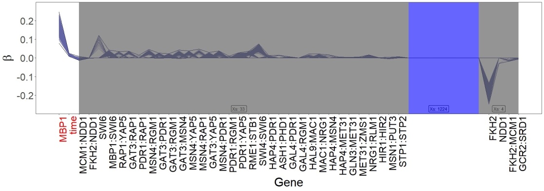
Figure 6: Graphical presentation of the SSCI (SPSP+AdaLasso) for the yeast cell-cycle data.

Table 3: Real data example: Yeast cell-cycle (G1) data

	$\text{SSCI}_{0.95}$
$\text{SSCI}_{0.95}$ (SPSP+AdaLasso)	Confidence intervals	Literature evidence		Effects documented in the literature
time	Significantly +++
MBP1	Significantly +++	Tsai et al., (2005), Wang et al., (2007), Yue et al., (2019)		+
SWI6	Plausibly +	Wang et al., (2007), Yue et al., (2019)		+
FKH2	Plausibly -	Tsai et al., (2005), Wang et al., (2007), Yue et al., (2019)		-
NDD1	Plausibly -	Tsai et al., (2005), Wang et al., (2007), Yue et al., (2019)		-
MBP1-SWI6	Plausibly +	Koch et al., (1993), Banerjee, (2003), Tsai et al., (2005)		+
MSN4-YAP5	Plausibly +	Banerjee, (2003), Tsai et al., (2005)		+
MSN4-PDR1	Plausibly +	Tsai et al., (2005)		+
SWI4-SWI6	Plausibly +	Koch et al., (1993), Banerjee, (2003), Tsai et al., (2005)		+
HAP4-PDR1	Plausibly +	Tsai et al., (2005)		+
HIR1-HIR2	Plausibly +	Loy et al., (1999), Banerjee, (2003)		NA
FKH2-MCM1	Plausibly -	Kumar et al., (2000), Banerjee, (2003)		NA
GAT3-PDR1	Plausibly	Banerjee, (2003), Tsai et al., (2005)		+
GAT3-MSN4	Plausibly	Banerjee, (2003)		NA
MCM1-NDD1	Plausibly	Kumar et al., (2000) Banerjee, (2003), Tsai et al., (2005)		-
FKH2-NDD1	Plausibly	Kumar et al., (2000), Banerjee, (2003), Tsai et al., (2005)		NA
	$\text{MCB}_{0.95}$
	Lower confidence bound model		Upper confidence bound model
SSCI (SPSP+AdaLasso)	{time, MBP1}		{time, MBP1, and all other plausible covariates}

We present the results of 95% SSCI in Figure 6. The upper and lower bounds of the confidence intervals are given in Table 3 of the supplementary materials. Among the 1263 covariates, only two covariates, MBP1 and time, are identified as significant covariates, deemed important for regulating the transcription process. Another 37 covariates are identified as plausible covariates, whose relevance to the gene expression levels requires further studies. The rest of the covariates are identified as unimportant. All covariates are displayed in Figure 6 using different shaded areas. Our results decrease the size of the candidate pool of biologically relevant TFs and synergistic interactions.

Comparing our results with the literature, all of our identified individual TFs, MBP1, FKH2, NDD1, and SWI6, are experimentally verified (Wang et al., , 2007). Besides, 12 of our identified cooperative TF pairs have been documented in the literature (MBP1-SWI6, GAT3-PDR1, GAT3-MSN4, MSN4-YAP5, MSN4-PDR1, SWI4-SWI6, HAP4-PDR1, GAL4-RGM1, HIR1-HIR2, MCM1-NDD1, FKH2-NDD1, FKH2-MCM1). The remaining 22 plausible TF pairs have either one or both TFs selected in the literature (Wang et al., , 2007) except the PDR1-RAP1 pair. We present some representative covariates from our SSCI in comparison to the literature in Table 3. A detailed comparison of all plausible covariates is given in Table 4 of the supplementary material.

For these plausible covariates, one advantage of SSCI is that it reports the possible sign of their effects if one of their boundaries is at zero, e.g., [0,1] or [-1,0]. We report the estimated signs of TFs as “plausibly +/-” in Table 3 and Table 4 of the supplementary materials and further compare the estimated signs with the documented regulatory effects in the literature. Most identified TFs and TF pairs (MBP1, FKH2, NDD1, SWI6, MBP1-SWI6, MSN4-YAP5, MSN4-PDR1, SWI4-SWI6, and HAP4-PDR1) are consistent with the literature (Tsai et al., , 2005).

6 Conclusion

This article proposes a sparse version of the simultaneous confidence intervals for high-dimensional linear regression. The proposed confidence intervals reflect rich information about the parameter and the model. Our approach has been theoretically and empirically justified, with desirable asymptotic properties and satisfactory numerical performance. There are many potential directions for future research. For example, we observe the varying performance of inference based on different variable selection methods. An interesting research topic would be to examine how applying different selection methods to the same data set might yield different results. Meanwhile, the weak signals pose challenges to many selection methods. Although we have tested our method numerically, extending our theoretical results to the weak signal case is an important topic (Liu et al., , 2020). In addition, our approach may be easily extended to build simultaneous confidence intervals for a subset of covariates, which is of great value in many real problems (Zhang and Cheng, , 2017).

SUPPLEMENTARY MATERIAL

Supplementary file:

The supplementary file (pdf) contains the algorithm of the residual bootstrap, details of two real data examples, and technical proofs. We demonstrate the SSCI on the low-dimensional Boston housing data. In addition, we include more details of the high-dimensional Yeast cell-cycle (G1) data analysis in the paper.

R-package for sparsified simultaneous confidence intervals:

We develop the R-package SSCI to construct and visualize the sparsified simultaneous confidence intervals described in the article. This package implements the SSCI method proposed in this paper and supports building the SSCI using all selection approaches adopted in simulation studies. (R package binary file)

On behalf of all authors, the corresponding author states that there is no conflict of interest.

References

- Banerjee, (2003) Banerjee, N. (2003). Identifying cooperativity among transcription factors controlling the cell cycle in yeast. Nucleic Acids Research, 31(23):7024–7031.
- Bühlmann and van de Geer, (2011) Bühlmann, P. and van de Geer, S. (2011). Statistics for High-Dimensional Data. Springer Series in Statistics. Springer Berlin Heidelberg, Berlin, Heidelberg.
- Cai and Guo, (2017) Cai, T. T. and Guo, Z. (2017). Confidence intervals for high-dimensional linear regression: Minimax rates and adaptivity. The Annals of Statistics, 45(2):615–646. Publisher: Institute of Mathematical Statistics.
- Chatterjee and Lahiri, (2011) Chatterjee, A. and Lahiri, S. N. (2011). Bootstrapping Lasso Estimators. Journal of the American Statistical Association, 106(494):608–625.
- Cheng and Li, (2008) Cheng, C. and Li, L. M. (2008). Systematic identification of cell cycle regulated transcription factors from microarray time series data. BMC Genomics, 9(1):116.
- Das et al., (2004) Das, D., Banerjee, N., and Zhang, M. Q. (2004). Interacting models of cooperative gene regulation. Proceedings of the National Academy of Sciences, 101(46):16234–16239.
- Dezeure et al., (2017) Dezeure, R., Bühlmann, P., and Zhang, C.-H. (2017). High-dimensional simultaneous inference with the bootstrap. TEST, 26(4):685–719.
- Efron, (1992) Efron, B. (1992). Bootstrap methods: another look at the jackknife. In Breakthroughs in statistics, pages 569–593. Springer.
- Fan and Li, (2001) Fan, J. and Li, R. (2001). Variable selection via nonconcave penalized likelihood and its oracle properties. Journal of the American statistical Association, 96(456):1348–1360.
- Fan and Lv, (2008) Fan, J. and Lv, J. (2008). Sure independence screening for ultrahigh dimensional feature space. Journal of the Royal Statistical Society: Series B (Statistical Methodology), 70(5):849–911.
- Ferrari and Yang, (2015) Ferrari, D. and Yang, Y. (2015). Confidence sets for model selection by f-testing. Statistica Sinica, pages 1637–1658.
- Freedman, (1981) Freedman, D. A. (1981). Bootstrapping Regression Models. The Annals of Statistics, 9(6):1218–1228.
- Hansen et al., (2011) Hansen, P. R., Lunde, A., and Nason, J. M. (2011). The Model Confidence Set. Econometrica, 79(2):453–497.
- Hastie and Qian, (2014) Hastie, T. and Qian, J. (2014). Glmnet vignette. Retrieved June, 9(2016):1–30.
- Inan and Wang, (2017) Inan, G. and Wang, L. (2017). PGEE: An R Package for Analysis of Longitudinal Data with High-Dimensional Covariates. The R Journal, 9(1):393.
- Javanmard and Montanari, (2014) Javanmard, A. and Montanari, A. (2014). Confidence intervals and hypothesis testing for high-dimensional regression. The Journal of Machine Learning Research, 15(1):2869–2909.
- Koch et al., (1993) Koch, C., Moll, T., Neuberg, M., Ahorn, H., and Nasmyth, K. (1993). A role for the transcription factors Mbp1 and Swi4 in progression from G1 to S phase. Science, 261(5128):1551.
- Kumar et al., (2000) Kumar, R., Reynolds, D. M., Shevchenko, A., Shevchenko, A., Goldstone, S. D., and Dalton, S. (2000). Forkhead transcription factors, Fkh1p and Fkh2p, collaborate with Mcm1p to control transcription required for M-phase. Current Biology, 10(15):896 – 906.
- Lee et al., (2016) Lee, J. D., Sun, D. L., Sun, Y., and Taylor, J. E. (2016). Exact post-selection inference, with application to the lasso. The Annals of Statistics, 44(3):907–927. arXiv: 1311.6238.
- Lee et al., (2002) Lee, T. I., Rinaldi, N. J., Robert, F., Odom, D. T., Bar-Joseph, Z., Gerber, G. K., Hannett, N. M., Harbison, C. T., Thompson, C. M., Simon, I., Zeitlinger, J., Jennings, E. G., Murray, H. L., Gordon, D. B., Ren, B., Wyrick, J. J., Tagne, J.-B., Volkert, T. L., Fraenkel, E., Gifford, D. K., and Young, R. A. (2002). Transcriptional regulatory networks in Saccharomyces cerevisiae. Science (New York, N.Y.), 298(5594):799–804.
- Li et al., (2019) Li, Y., Luo, Y., Ferrari, D., Hu, X., and Qin, Y. (2019). Model confidence bounds for variable selection. Biometrics, 75(2):392–403.
- Liu et al., (2020) Liu, H., Xu, X., and Li, J. J. (2020). A Bootstrap Lasso + Partial Ridge Method to Construct Confidence Intervals for Parameters in High-dimensional Sparse Linear Models. Statistica Sinica.
- Liu and Wang, (2018) Liu, Y. and Wang, P. (2018). Selection by partitioning the solution paths. Electronic Journal of Statistics, 12(1):1988–2017.
- Lockhart et al., (2014) Lockhart, R., Taylor, J., Tibshirani, R. J., and Tibshirani, R. (2014). A significance test for the lasso. Annals of statistics, 42(2):413–468.
- Loy et al., (1999) Loy, C. J., Lydall, D., and Surana, U. (1999). NDD1 , a High-Dosage Suppressor of cdc28-1N , Is Essential for Expression of a Subset of Late-S-Phase-Specific Genes in Saccharomyces cerevisiae. Molecular and Cellular Biology, 19(5):3312–3327.
- Luan and Li, (2003) Luan, Y. and Li, H. (2003). Clustering of time-course gene expression data using a mixed-effects model with B-splines. Bioinformatics, 19(4):474–482.
- Ma et al., (2021) Ma, R., Tony Cai, T., and Li, H. (2021). Global and Simultaneous Hypothesis Testing for High-Dimensional Logistic Regression Models. Journal of the American Statistical Association, 116(534):984–998.
- Nan and Yang, (2014) Nan, Y. and Yang, Y. (2014). Variable Selection Diagnostics Measures for High-Dimensional Regression. Journal of Computational and Graphical Statistics, 23(3):636–656.
- Qin et al., (2022) Qin, Y., Wang, L., Li, Y., and Li, R. (2022). Visualization and assessment of model selection uncertainty. Computational Statistics & Data Analysis.
- Scheffé, (1953) Scheffé, H. (1953). A method for judging all contrasts in the analysis of variance. Biometrika, 40(1-2):87–110. Publisher: Oxford University Press.
- Shi and Qu, (2017) Shi, P. and Qu, A. (2017). Weak signal identification and inference in penalized model selection. The Annals of Statistics, 45(3):1214–1253.
- Spellman et al., (1998) Spellman, P. T., Sherlock, G., Zhang, M. Q., Iyer, V. R., Anders, K., Eisen, M. B., Brown, P. O., Botstein, D., and Futcher, B. (1998). Comprehensive Identification of Cell Cycle–regulated Genes of the Yeast Saccharomyces cerevisiae by Microarray Hybridization. Molecular Biology of the Cell, 9(12):3273–3297.
- Tibshirani, (1996) Tibshirani, R. (1996). Regression shrinkage and selection via the lasso. Journal of the Royal Statistical Society: Series B (Methodological), 58(1):267–288.
- Tibshirani et al., (2016) Tibshirani, R. J., Taylor, J., Lockhart, R., and Tibshirani, R. (2016). Exact Post-Selection Inference for Sequential Regression Procedures. Journal of the American Statistical Association, 111(514):600–620.
- Tsai et al., (2005) Tsai, H.-K., Lu, H. H.-S., and Li, W.-H. (2005). Statistical methods for identifying yeast cell cycle transcription factors. Proceedings of the National Academy of Sciences, 102(38):13532–13537.
- van de Geer et al., (2011) van de Geer, S., Bühlmann, P., Zhou, S., et al. (2011). The adaptive and the thresholded lasso for potentially misspecified models (and a lower bound for the lasso). Electronic Journal of Statistics, 5:688–749.
- van de Geer et al., (2014) van de Geer, S., Bühlmann, P., Ritov, Y., and Dezeure, R. (2014). On asymptotically optimal confidence regions and tests for high-dimensional models. The Annals of Statistics, 42(3).
- Wang et al., (2007) Wang, L., Chen, G., and Li, H. (2007). Group SCAD regression analysis for microarray time course gene expression data. Bioinformatics, 23(12):1486–1494.
- Wang et al., (2021) Wang, L., Qin, Y., and Li, Y. (2021). Confidence graphs for graphical model selection. Statistics and Computing.
- Wang et al., (2012) Wang, L., Zhou, J., and Qu, A. (2012). Penalized Generalized Estimating Equations for High-Dimensional Longitudinal Data Analysis. Biometrics, 68(2):353–360.
- Wickham, (2011) Wickham, H. (2011). ggplot2. Wiley Interdisciplinary Reviews: Computational Statistics, 3(2):180–185. Publisher: Wiley Online Library.
- Yuan and Guo, (2022) Yuan, P. and Guo, X. (2022). High-dimensional inference for linear model with correlated errors. Metrika, 85(1):21–52.
- Yue et al., (2019) Yue, M., Li, J., and Cheng, M.-Y. (2019). Two-step sparse boosting for high-dimensional longitudinal data with varying coefficients. Computational Statistics & Data Analysis, 131:222 – 234.
- Zhang and Zhang, (2014) Zhang, C.-H. and Zhang, S. S. (2014). Confidence intervals for low dimensional parameters in high dimensional linear models. Journal of the Royal Statistical Society: Series B (Statistical Methodology), 76(1):217–242.
- Zhang and Cheng, (2017) Zhang, X. and Cheng, G. (2017). Simultaneous Inference for High-Dimensional Linear Models. Journal of the American Statistical Association, 112(518):757–768.
- Zhang et al., (2010) Zhang, Y., Li, R., and Tsai, C.-L. (2010). Regularization parameter selections via generalized information criterion. Journal of the American Statistical Association, 105(489):312–323.
- Zhao and Yu, (2006) Zhao, P. and Yu, B. (2006). On model selection consistency of lasso. Journal of Machine learning research, 7(Nov):2541–2563.
- (48) Zheng, C., Ferrari, D., and Yang, Y. (2019a). Model selection confidence sets by likelihood ratio testing. Statistica Sinica.
- (49) Zheng, C., Ferrari, D., Zhang, M., and Baird, P. (2019b). Ranking the importance of genetic factors by variable-selection confidence sets. Journal of the Royal Statistical Society. Series C. Applied Statistics, 68(3):727–749.