Harpa: High-Rate Phase Association with Travel Time Neural Fields

Our understanding of regional seismicity from multi-station seismograms relies on the ability to associate arrival phases with their originating earthquakes. Deep-learning-based phase detection now detects small, high-rate arrivals from seismicity clouds, even at negative magnitudes. This new data could give important insight into earthquake dynamics, but it is presents a challenging association task. Existing techniques relying on coarsely approximated, fixed wave speed models fail in this unexplored dense regime where the complexity of unknown wave speed cannot be ignored. We introduce Harpa, a high-rate association framework built on deep generative modeling and neural fields. Harpa incorporates wave physics by using optimal transport to compare arrival sequences. It is thus robust to unknown wave speeds and estimates the wave speed model as a by-product of association. Experiments with realistic, complex synthetic models show that Harpa is the first seismic phase association framework which is accurate in the high-rate regime, paving the way for new avenues in exploratory Earth science and improved understanding of seismicity.

Teaser

Physics-informed generative ML enables very high rate seismic phase association despite large wavespeed uncertainty.

Introduction

Seismic signals are a gateway to understanding the structure and dynamics of the Earth. Recent breakthroughs in deep-learning-based seismic processing enable reliable detection of very small, high-rate seismic events  (?, ?, ?) with potential to reveal unprecedented details about the variability of elastic material properties in the Earth’s crust and upper mantle. Progress is, however, stymied by the limitations of existing phase association methodologies designed for larger events which are less frequent, following the Gutenberg–Richter law. High arrival rates such as those associated with seismic clouds  (?) pose unique challenges.

This highly-interleaved regime is illustrated in Fig. 1. When waves from many seismic events arrive topsy-turvy at the stations at similar times, associating them to their originating events is challenging even if the wave speed model is known or can be approximated by a simple model (constant or 1-d). In reality, however, even the wave speed models are not known, certainly not so at the required resolution. This uncertainty further exacerbates the difficulty of associating and locating earthquakes, making it essential to develop methods which work in this challenging high-rate regime and handle unknown wave speeds.

To address this gap we propose Harpa—a method that can solve the high-rate association problem over an unknown wave speed in settings considerably more complex than those addressed by existing methods. Harpa first solves a seemingly harder problem: estimating locations and occurrence times of earthquakes jointly with an (approximate) wave speed model.

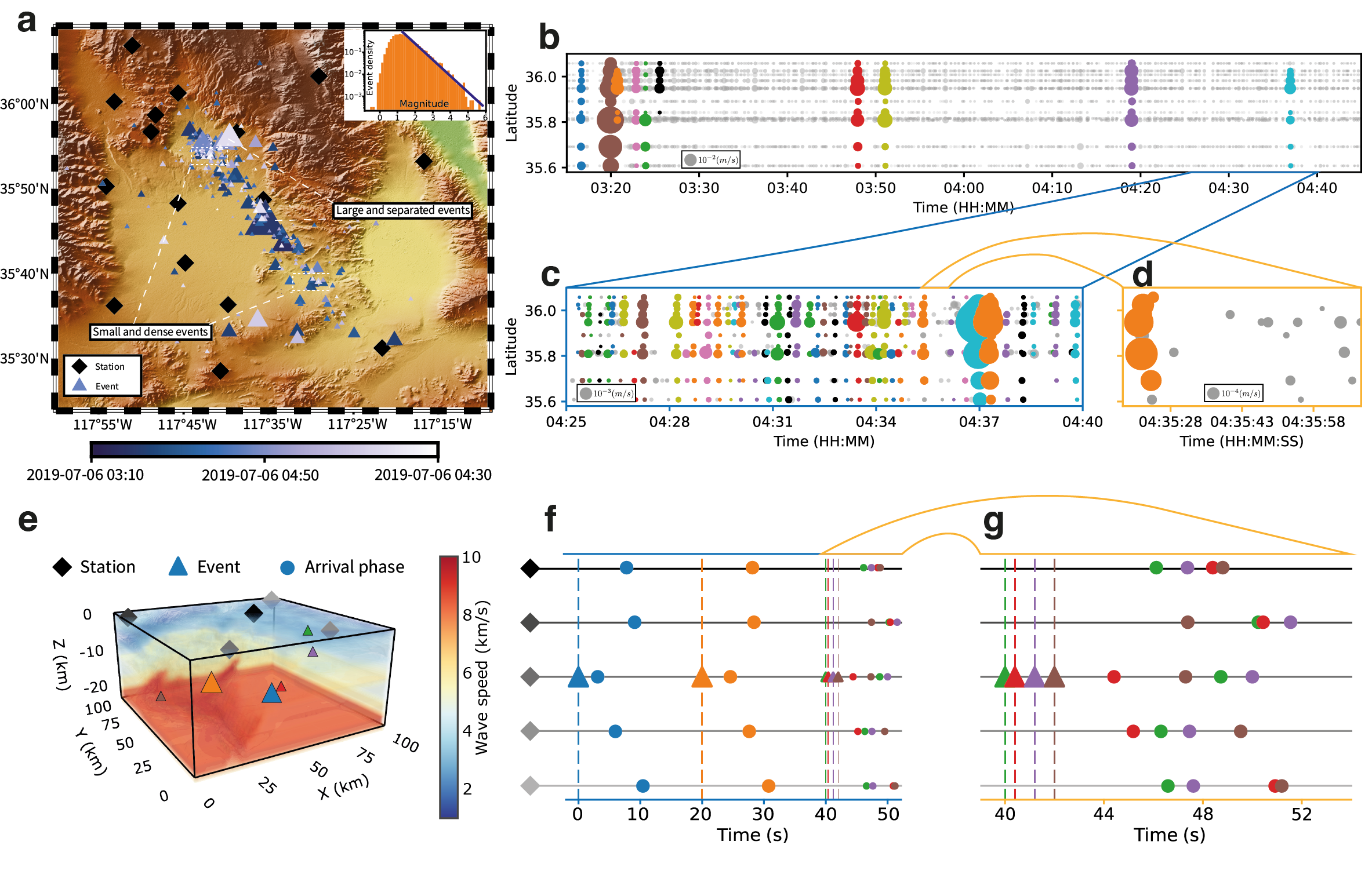
Figure 1: Seismic events on different time scales and magnitudes: Panel a: seismic data from Ridgecrest CA, recorded on July 6, 2019, between 04:10 and 04:30. It has both large, isolated events and small, clustered ones. Triangle sizes represent earthquake magnitudes; color represents arrival times. The density distribution of magnitudes illustrated in the inset plot signifies the Gutenberg-Richter law where the slope represents the $b$ value. Panel b: low-rate large magnitude events which are easy to associate. Each trace on the plot corresponds to a recording from a station, which is positioned according to its respective latitude value on the y-axis. The diameters of the disks are indicative of the peak ground velocity (PGV)  (?). Color represents the association, that is, waveforms from a common seismic source. Gray disks in c, d indicate the unidentified arrivals in  (?). Large magnitude arrivals in panel b are straightforwardedly linked. Panel c illustrates a time interval, at finer scale, that is more challenging for association but nonetheless successful as the arrival time fluctuations due to the henetrogeneity in wavespeed are still small compared to the intermittancy (rate) of events. At yet a finer time scale and shorter interval in panel d identification and association becomes a challenge and has, by traditional techniques, been unresolved. This intermittancy or rates originate from yet smaller earthquakes in accordance with the Gutenberg-Richter law. On the one hand, the detection of ever smaller events is challenging due to “background” noise; on the other hand, the implied increasing rate poses the challenge of association due to wavespeed fluctuations. It is the latter that we address and illustrate in panels e, f, and g. Here, we demonstrate this using a synthetic wave speed model, the SEG/EAGE 3-D overthrust, with congruent spatial dimensions. Blue and orange triangles indicate two earthquakes occurring 20 seconds apart, with easily associated arrivals (panel g). The remaining four smaller triangles indicate events which all occur within 2 seconds, presenting a significantly harder association challenge where the ordinal number of arrival carries no significance (panel g). It is worthwhile noting that under stronger wave speed fluctuations the association challenge addressed here appears at larger magnitude earthquakes.

Only then does it assign earthquake phases, but with the estimated earthquake and wave speed parameters the problem reduces to a simpler linear assignment problem. This simplification is afforded by leveraging the physics of wave propagation and advances in generative modeling and optimal transport.

Indeed, while the traditional localization methods rely on associated phases, we sidestep this requirement by interpreting the arrival time data at each station as a probability measure, and using optimal transport to quantify the discrepancy between the measures corresponding to the observed data and to our estimates.

There are two major challenges in implementing this program. The first is to enable numerically efficient differentiable optimization with respect to source locations and wave speed models which respects propagation physics. This is difficult with traditional mesh-based eikonal solvers; scaling to 3D would result in prohibitive computational complexity (?). The second challenge lies in finding the globally optimal solution of the associated non-convex optimization problem. While the problem of wave speed reconstruction from unknown sources admits a unique solution under certain conditions  (?), identifying this solution by optimizing a non-convex objective is challenging due to the presence of poor local minima.

To resolve the first challenge, we first train a deep generative model to embed a family of complex wave speeds in a low-dimensional latent space and optimize the latent code of the wave speed and the spatio-temporal earthquake parameters simultaneously. But instead of directly addressing the formidable challenge of optimizing these parameters through a numerical solver we train a deep neural field  (?, ?, ?) to fit the travel times between arbitrary interior points and a fixed set of receivers. An autoencoder structures the latent space and provides a pairing between latent codes and wave speeds which is then used by the travel time neural field. As we show in Experiments, fitting the best wave speed from the range of a sufficiently diverse generative model makes the association highly robust, even when the test wave speed is far out of the distribution used to train the model.

To resolve the second challenge, we leverage a combination of stochastic gradient-based methods and sampling. Markov Chain Monte Carlo (MCMC) methods can in principle deal with the non-convexity but they are ineffective in our setting because the search space is too large. We employ Stochastic Gradient Langevin Dynamics (SGLD)  (?) to ensure an adequate exploration of the loss landscape by the gradient optimizer, ultimately leading to the identification of a (near-)global optimum.

We test Harpa on a suite of challenging computer experiments, on complex unknown wave speeds and with extremely dense seismic events which arrive at different stations in completely different sequences. We demonstrate for the first time accurate and robust phase association in this regime. We show that Harpa remains robust in the face of realistic wave speed distortions and noisy or missing arrival picks at the stations, suggesting exciting new avenues in exploratory Earth science. All results in this paper are fully reproducible.

Background and related work

If earthquake source locations, occurrence times, and wave speeds are all known, the phase association problem can be formulated as a linear sum assignment problem (LSAP), which is effectively solved by the Hungarian algorithm  (?). If only the occurrence times are unknown, the problem is related to a quadratic assignment problem (QAP)  (?, ?) which is NP-hard. While QAPs can be solved in certain practical cases using heuristics and meta-heuristics  (?, ?), there has been growing interest in leveraging machine learning to solve similar combinatorial optimization problems  (?, ?, ?). The situation, however, is often even more complex: neither the wave speed nor the spatiotemporal earthquake source locations are known, although sometimes a rather coarse wave speed model is available. These unknown degrees of freedom result in a mixed-integer programming problem which is harder than LSAP or QAP and challenging to solve even with a small number of earthquakes and stations  (?, ?, ?).

Although the joint localization–wave speed recovery problem has a unique solution under certain conditions  (?), there are no reliable algorithms that solve it provably and efficiently. Notwithstanding, there exist algorithmic attempts to perform joint full waveform (or sometimes travel time) inversion and wave speed model refinement but with temporally well-separated sources, thus implicitly avoiding the association problem (while still facing the ill-posedness)  (?, ?, ?). In the context of micro-seismicity, simple parametric models  (?) and Bayesian priors  (?) were used for regularization. We mention that our strategy to convert combinatorial data into measures in order to avoid combinatorial optimization is reminiscent of earlier work on unassigned Euclidean distance data  (?, ?) with applications in genomics and room acoustics.

Over the last decade there has been an increasing interest in the application of machine learning in seismology, for example for phase picking  (?, ?, ?, ?). A multitude of studies addressing the phase association problem have employed either probabilistic   (?, ?, ?) or graph models  (?, ?). Some adopt a static or 1-D wave speed model, while others incorporate wave speed information indirectly through supervised learning. Since these approaches do not explicitly leverage the wave propagation physics they demand large quantities of data for training. All phenomena in the association problem are governed by the wave equation which is known, but is typically only leveraged for downstream analysis once the phases have been associated. We show that rethinking the problem in measure-theoretic terms allows one to leverage the wave propagation model from the outset.

Results

Problem formulation

We consider an unknown wave speed $c:\Omega\to\mathbb{R}^{+}$ where $\Omega\subset\mathbb{R}^{3}$ is the domain of interest that contains sources and ray paths. For a given $c$, we use $T_{c}(s;r)$ to represent the time it takes for a wave to travel from source point $s\in\Omega$ to a boundary receiver point $r\in\partial\Omega$. We assume there are $N$ stations and $M$ sources. Each source generates one event, and we assume that each station receives $K$ phases originating from the $M$ sources. (We first assume $K=M$ and later discuss situations with noisy and missing picks where $K\neq M$.) We let $\mathcal{R}=\left\{r_{i}\in\Omega\mid i\leq N\right\}$ be the set of the $N$ stations locations. Arrival time data recorded at each station is denoted by $\mathcal{D}_{i}=\{t_{i,k}\mid k\leq M\}$, where $t_{i,k}$ represents the arrival time for each pick. For a given fixed time window, we observe earthquakes with spatio-temporal locations $\mathcal{E}=\{(s_{j},\tau_{j})\mid s_{j}\in\Omega,\tau_{j}\in[0,\tau_{\mathrm{max}}),j\leq M\}$. If an earthquake with location and occurrence time $e_{j}=(s_{j},\tau_{j})$ is observed as the $k$-th arrival at station $i$ with arrival time $t_{i,k}$, we have

$$t_{i,k}=T_{c}(s_{j};r_{i})+\tau_{j}.$$ (1)

The goal of the source–receiver association is to determine which picks correspond to which source. To model this, we define the ground truth association as

$$\alpha^{*}(k;r_{i}):=j\leq M,$$

and its corresponding inverse assignment as

$${\alpha^{*}}^{-1}(j;r_{i}):=k\leq M.$$

A mixed-integer optimization problem

We aim to infer the assignment $\alpha^{*}$ (up to a global permutation), the unknown wave speed $c^{*}$, and the source locations and times $\mathcal{E}^{*}$, from arrival time data. This can be formulated as the following mixed-integer optimization problem,

$$\underset{\alpha,c,\mathcal{E}}{\operatorname{minimize}}\quad L(\alpha;c,\mathcal{E}),$$ (2)

where the loss function is defined using a suitable discrepancy metric $\ell(a,b)$ on the arrival times,

$$L(\alpha;c,\mathcal{E})=\sum_{j\leq M,i\leq N}\ell\left(T_{c}\left(s_{j};r_{i}\right)+\tau_{j},\leavevmode\nobreak\ t_{i,\alpha^{-1}(j;r_{i})}\right).$$ (3)

We mention in the passing that some works deal with the unknown occurrence times by using time difference of arrival (TDoA) data instead of including the takeoff times as optimization variables; this is achieved by minimizing the mismatch loss

$$L^{M}(\alpha;c,\mathcal{E})=\sum_{j\leq M,i_{a}<i_{b}\leq N}\ell\left(T_{c}\left(s_{j};r_{i_{a}}\right)-T_{c}\left(s_{j};r_{i_{b}}\right),\leavevmode\nobreak\ t_{i_{a},\alpha^{-1}(j;r_{i_{a}})}-t_{i_{b},\alpha^{-1}(j;r_{i_{b}})}\right).$$ (4)

Since we also recover the takeoff times we work directly with ToAs.

Generative modeling of low-dimensional wave speed families

To build Harpa we assume that the wave speed models and consequently travel times exhibit a latent low-dimensional structure. We thus model the wave speeds by an autoencoder-based generative model and traveltimes by a matching continuous coordinate-based neural field  (?, ?, ?). The assumption of latent low-dimensionality is consistent with geodynamical models which generate the distribution of the elastic material properties in the interior; this has been explored for Earth’s mantle before  (?, ?). Geological random fields have been used to in conjuction with accurate earthquake simulations to study the 2019 Le Teil earthquake in a region where little geophysical data is available  (?). In fact, the wave speeds generated by our latent model ($\mathbb{R}^{L}\ni z\mapsto c(z)$) are considerably more complex than the fixed models used for association in the recent literature which only vary along the depth coordinate  (?, ?, ?). We thus define the associated travel time function as $T(s,z;r)=T_{c}(s;r)$. This enables us to rewrite the optimization problem involving $c$ as one involving the latent code $z$,

$$\underset{\alpha,z,\mathcal{E}}{\operatorname{minimize}}\quad L(\alpha;c(z),\mathcal{E}).$$ (5)

Association without association

For a known wave speed and spatio-temporal source locations, and in the absence of error in travel time estimates, the optimal assignment $\alpha^{*}$ yields $L(\alpha^{*})=0$ in (2). This assignment can thus be obtained simply as

$$\alpha(j,r_{i})=\operatorname*{arg\,min}_{k}\leavevmode\nobreak\ \ell(T_{c}(s_{j};r_{i})+\tau_{j},\leavevmode\nobreak\ t_{i,k}).$$ (6)

Instead of directly addressing phase association, we first solve a seemingly harder (approximate) joint recovery problem. We map the arrival times $\mathcal{D}_{i}$ to a discrete probability measure

$$\rho_{i}=\frac{1}{M}\sum_{k=1}^{M}\mathbbm{1}_{\{t_{i,k}\}}$$ (7)

which we regard as the ground truth probability measure. By “passing through the wave equation” we can similarly construct a discrete probability measure for any wave speed latent code $z$ and earthquake sources with parameters $\mathcal{E}$,

$$\rho_{i}^{\mathcal{E},z}=\frac{1}{M}\sum_{e_{j}\in\mathcal{E}}\mathbbm{1}_{\{T(s_{j},r_{i},z)+\tau_{j}\}},$$ (8)

We aim to align these two measures by minimizing their Wasserstein distance defined for $p\geq 1$ as

$$w_{p}(\rho_{1},\rho_{2})=\left(\inf_{\gamma\in\mathcal{C}\left(\rho_{1},\rho_{2}\right)}\int|{\theta}_{1}-{\theta}_{2}|^{p}\gamma\left(\mathrm{d}{\theta}_{1},\mathrm{\leavevmode\nobreak\ d}{\theta}_{2}\right)\right)^{1/p}.$$ (9)

In the case where some phase picks are missing or spurious picks are present, we define a loss for matching unbalanced arrivals based on sparsity-constrained optimal transport; a detailed description is given in Materials and method and results in Fig. 9c. In the 1-dimensional discrete case this loss coincides with the Wasserstein loss of the unbalanced linear assignment.

The source locations and times can finally be estimated by optimizing the following loss (cf. Fig. 2),

$$\underset{\mathcal{E},z}{\mathrm{minimize}} \quad W(\mathcal{E},z)$$ (10)

where $$\quad\sum_{i=1}^{N}w_{p}(\rho^{\mathcal{E},z}_{i},\rho_{i})\quad\text{and}\quad\rho^{\mathcal{E},z}_{i}=\frac{1}{M}\sum_{e_{j}\in\mathcal{E}}\mathbbm{1}_{\{T(s_{j},z;r_{i})+\tau_{j}\}}.$$

What this passing to measures affords us is invariance to permutations of arrivals. In other words, it removes the need for association. We can relate (10) to (2) where we explicitly sought the optimal assignment $\alpha^{*}$ as follows. In the noiseless setting, we have

$$\rho_{i}^{\mathcal{E}^{*},z^{*}}=\frac{1}{M}\sum_{k}\mathbbm{1}_{\{T_{c^{*}}(s^{*}_{(\alpha^{*})^{-1}(k;r_{i})};r_{i})+\tau^{*}_{{(\alpha^{*})}^{-1}(k;r_{i})}\}},$$

where $\mathcal{E}^{*},z^{*}$ on the left hand side are the solution of (10) while $c^{*},\alpha^{*},(s^{*},\tau^{*})$ on the right hand side are the solution of (2). After obtaining $\mathcal{E}^{*}=(s^{*},\tau^{*})$ from (10), we can find $\alpha^{*}$ by solving LSAP directly, or by using only $s^{*}$ without $\tau^{*}$ by solving the TDoA problem as in (4)).

We assume that earthquakes are well-approximated by point sources which are distributed volumetrically so that we obtain sufficiently rich data. These conditions are satisfied in reality with events occurring close to ensembles of faults (or fractures) at varying orientations, or in “clouds”  (?, ?).

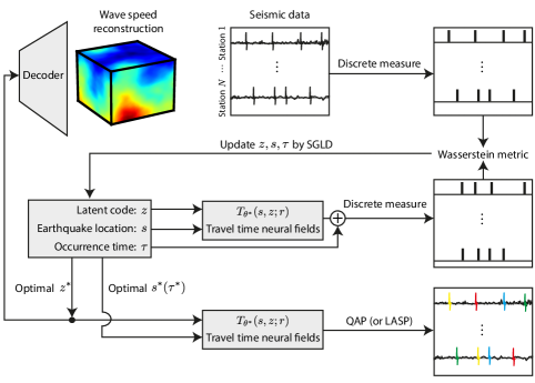
Figure 2: Diagram of Harpa’s association pipeline.

Generative travel time neural fields

The complexity of solving (10) strongly depends on the complexity of computing the travel time function $T(s,z;r)$. For a given wave speed (or its latent code $z$) we can use a standard numerical solver to obtain the value of $T$ at a desired set of points.

This, however, poses major challenges: numerical solvers work on grids or meshes; we would like to use continuous optimization to optimize source locations which is far from straightforward with a fixed discrete grid. Even if we circumvent the grid issue, taking gradients to use differentiable optimization would require us to differentiate $T$ both with respect to the source location and with respect to the latent code $z$. In that case, the computational complexity of differentiating through an iterative solver would result in a prohibitively complex method.

The way we resolve this conundrum in Harpa is as follows: We first use a deep autoencoder to build a low-dimensional latent representation of a set of complex wave speeds; see Experiments and Fig. 3. Next, we use the fast marching method as implemented in scikit-fmm to compute the travel times between a fixed set of receivers and sources at each possible mesh node. The final and key step is then to fit a neural field (also known as an implicit neural representation) to the travel time data  (?, ?). We use a neural network $T_{\theta}$ with weights $\theta$ and periodic activation functions  (?) which ensures that travel times and their derivatives with respect to source locations and wave speed latent codes can be efficiently evaluated at continuous coordinates. We train $T_{\theta}$ so that $T_{\theta^{*}}(s,z;r)\approx T(s,z;r)$ fits the travel time at a discrete set of grid points in space,

$$\theta^{*}=\operatorname*{arg\,min}_{\theta}\sum_{z\in\mathcal{Z},s\in\mathcal{S},r\in\mathcal{R}}(T(s,z;r)-T_{\theta}(s,z;r))^{2},$$ (11)

where $\mathcal{Z}$ denotes the set of sampled wave speeds (that is to say, their corresponding latent codes), $\mathcal{S}$ represents the set of coordinates in the spatial domain (typically chosen as a grid), and $T(s,z;r)$ is pre-computed using a numerical solver. The latent travel time neural field, which mimics the real travel time function, provides a continuous representation of the travel time which is differentiable with respect to both $s$ and $z$, thus enabling gradient-based optimization.

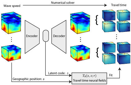
Figure 3: Diagram of the wave speed autoencoder and the travel time neural field.

The Wasserstein loss in (10) is differentiable with respect to both $z$ and $\mathcal{E}$ but it is not convex in these parameters which means that local gradient-based optimization may converge to local minima. The total number of parameters, $(3+1)\times N+L$, is small compared with common deep neural networks so there is no reason to expect that these local minima are benign. Indeed, as shown in Materials and method, we observe empirically that stochastic gradient descent (SGD) often converges to poor local minima in this setting. Monte Carlo as an alternative would be prohibitively slow.

There exist modern iterative optimizers which combine the favorable aspects of sampling methods and SGD. A notable example is stochastic gradient Langevin dynamics (SGLD)  (?), which can be viewed either as a mini-batch variant of Langevin dynamics or as a noisy SGD. The global convergence of Langevin dynamics can be leveraged to locate the globally-optimal earthquake and wave speed parameters which approximate their corresponding ground truth values, while benefiting from fast convergence rates  (?, ?); here the (relatively) small number of parameters helps. A SGLD iterate is computed as

$$z \leftarrow z-\eta\widehat{\nabla_{z}W}+\sqrt{2\eta}\epsilon\xi_{z},$$ (12)

$$s \leftarrow s-\eta\widehat{\nabla_{s}W}+\sqrt{2\eta}\epsilon\xi_{s},$$

$$\tau \leftarrow\tau-\eta\widehat{\nabla_{\tau}W}+\sqrt{2\eta}\epsilon\xi_{\tau},$$

where $\eta$ is the step size, and $\widehat{\nabla W}$ is a mini-batch sum in (10) which is an unbiased estimator of the gradient $\nabla W$. The parameter $\epsilon$ modulates the amplitude of noise; $\xi_{z}$, $\xi_{s}$, and $\xi_{\tau}$ are standard normal vectors independently drawn across different iterations from a Gaussian distribution with mean zero and variance one.

Experiments

We now showcase the performance of Harpa on a suite of computer experiments; we work with both known and unknown wave speeds. In Association via joint recovery we first test the limits of Harpa on a challenging set of unknown wave speeds in terms of the numbers of sources and receivers and show successful association in a variety of settings which were heretofore inaccessible for association. In Distorted and out-of-distribution wave speeds we apply Harpa to realistic wave speed models derived from the SEG / EAGE 3-D overthrust model  (?) which come from a different distribution than the one used to train the latent wave speed model and show that the proposed method is robust to such perturbations. Finally, in Spurious and missing picks we demonstrate robustness to spurious and missing phase picks.

Confusion factor and association evaluation

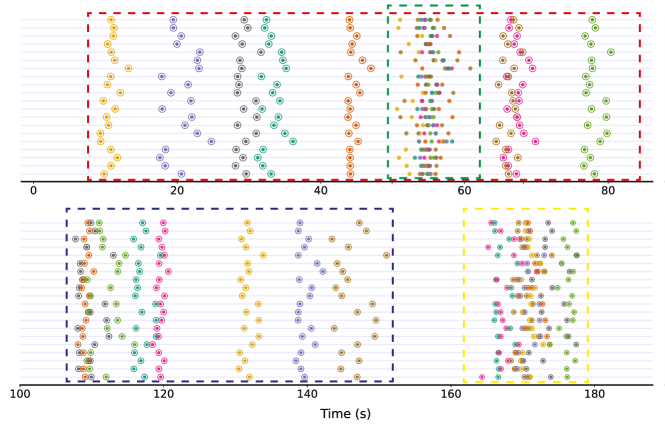
Figure 4: Phase association for different arrival rates / confusion factors. Each colored frame contains 8 sources recorded by 20 stations. Each horizontal line represents a stations, with colored circles representing arrivals. The inner circle color encodes the ground truth association; the outer circle color encodes association computed by Harpa. Green: $\mathsf{CF}=0.88$, $\mathsf{ACC}=97.5\%$, $e_{l}=0.04$ s; yellow: $\mathsf{CF}=0.42$, $\mathsf{ACC}=98.8\%$, $e_{l}=0.03$ s; navy blue: $\mathsf{CF}=0.05$, $\mathsf{ACC}=100\%$, $e_{l}=0.02$ s; red: $\mathsf{CF}=0.02$, $\mathsf{ACC}=100\%$, $e_{l}=0.03$ s.

To quantify the level of disorder in seismic event arrivals, and to compare the difficulty of joint inference and association problems, we define the confusion factor (CF) which ranges from 0 to 1. A value close to 0 indicates that the picks arrive in a similar order across stations and is easy for association (e.g., red box in Fig. 4). Conversely, a value close to 1 indicates that the picks arrive in a confused manner (e.g., green box in Fig. 4). The CF is mathematically defined as follows:

$$\mathsf{CF} =1-\max\left\{\frac{1}{N}\sum_{i=1}^{N}\mathcal{T}\left[\{(T_{c}(s_{j};r_{i})+\tau_{j},\leavevmode\nobreak\ \tau_{j})\}_{j=1}^{M}\right],0\right\}$$ (13)

$$=1-\max\left\{\frac{1}{N}\sum_{i=1}^{N}\mathcal{T}\left[\{(t_{i,\alpha^{*}(j;r_{i})},\tau_{j})\}_{j=1}^{M}\right],0\right\},$$

where

$$\mathcal{T}\left[\left\{(a_{j},b_{j})\right\}_{j}\right]=\frac{\text{number of concordant pairs}-\text{number of discordant pairs}}{\text{number of pairs}}$$

calculates Kendall’s $\tau$ rank correlation coefficient  (?). Succinctly, when the order of the arrivals at a station matches the order of earthquake occurrences, $\mathcal{T}$ yields a value of $1$ and $\mathsf{CF}=0$. This typically occurs during low-rate earthquakes, where the travel time is shorter than the time between the different events. Conversely, when all earthquakes occur almost simultaneously, the order of earthquake occurrence bears no correlation with the order of the phases/picks arriving at the stations. This reduces $\mathcal{T}$ closer to $0$, and pushes $\mathsf{CF}$ closer to $1$, implying a higher level of confusion (the $\mathsf{CF}$ is always between 0 and 1). When studying regions such as Ridgecrest around the time of the 2019 earthquake, the magnitude cutoff is usually chosen so that the resulting CF is below 0.1  (?, ?, ?). Fig. 4 shows representative arrival configurations for different values of $\mathsf{CF}$; Fig. 9 shows results of an exhaustive test of the proposed method at different $\mathsf{CF}$.

The difficulty of association is not solely determined by $\mathsf{CF}$; it also depends on the number of stations $N$ and the number of sources $M$ being simultaneously associated. Many algorithms initially partition the data into shorter temporal windows, usually between 5 and 20 seconds in length, with approximately 5 to 20 events in each window  (?, ?). In this proof of concept work we focus on a single window.

To characterize performance we also record the phase association accuracy defined as

$$\mathsf{ACC}=\frac{1}{NM}\sum_{i=1}^{N}\sum_{j=1}^{M}\delta\left(\alpha(j;r_{i}),\alpha^{*}(j;r_{i})\right)$$ (14)

where $\delta$ is the Kronecker delta. When the squared difference metric $\ell(a,b)=(a-b)^{2}$ is used in (3), we use $e_{l}=\sqrt{L(\alpha;c(z),\mathcal{E})/(MN)}$ to characterize the error in arrival time as a consequence of misassociation.

Association via joint recovery

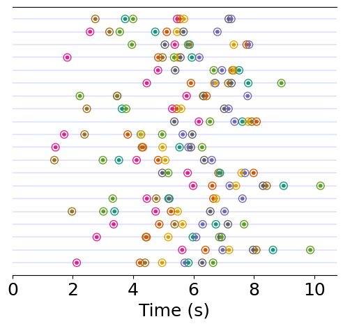
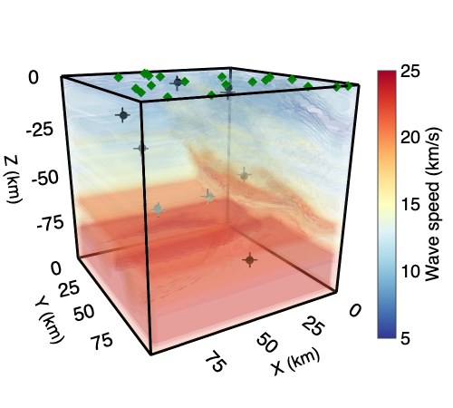
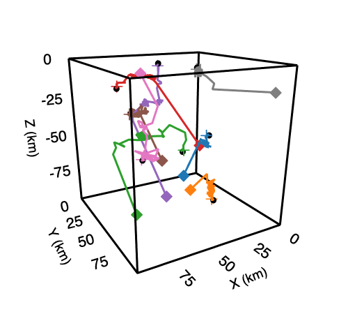
Figure 5: Association results for $8$ sources, $20$ stations and $\mathsf{CF}=0.93$ with SEG/EAGE 3-D overthrust model as the known wave speed. Harpa achieves $\mathsf{ACC}=95.0\%$ and $e_{l}=0.03$ s. Left: each horizontal line represents the arrivals at one station. Inner circles show the correct association, and the outer circles show the association results of Harpa. Middle: color corresponds to the wave speed; green diamonds, black crosses, and black circles represent station locations, predicted earthquake locations, and ground truth earthquake locations, respectively. Right: source trajectories during SGLD-based learning; diamond markers are initial locations, cross markers are stopping points after $100$ epochs.

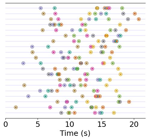
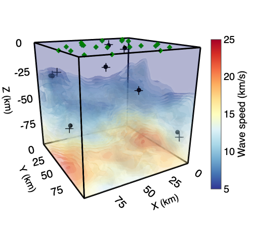
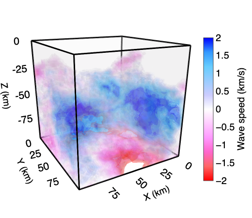
Figure 6: Association results for $8$ sources, $20$ stations and $\mathsf{CF}=0.94$ with unknown wave speed. Harpa achieves $\mathsf{ACC}=91.3\%$ and $e_{l}=0.07$ s. Left: each horizontal line represents the arrivals at one station. Inner circles show the correct association, and the outer circles show the association results of Harpa. Middle: wave speed recovered by Harpa. Right: difference between the recovered and ground truth wave speed. Definitions of symbols are as in Fig. 5.

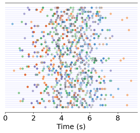
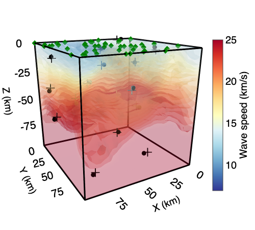
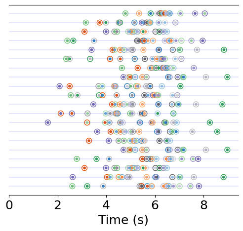
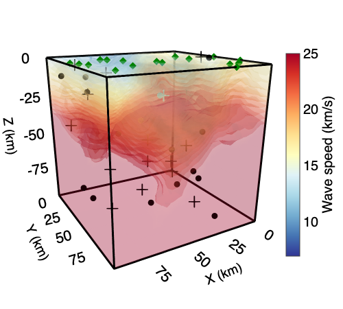
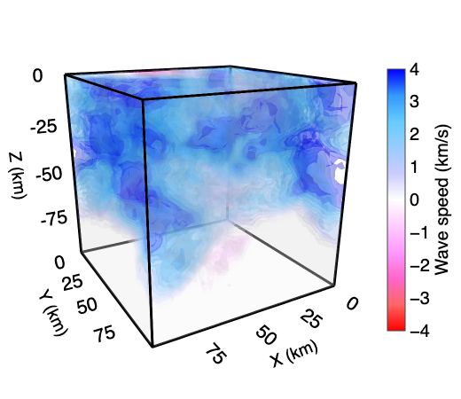
Figure 7: Association results for $16$ sources with $20$ and $50$ stations. Top row (50 stations): $\mathsf{ACC}=72.0\%$, $e_{l}=0.10$ s, $\mathsf{CF}=0.98$ ). Bottom row (20 stations): $\mathsf{ACC}=28.4\%$, $e_{l}=0.29$ s $\mathsf{CF}=0.90$. Symbols and encoding are as in Fig. 6.

We simulate wave propagation in a region of size $100$ km $\times$ $100$ km $\times$ 100 km, with wave speeds ranging from $5$km/s to $25$km/s. We assume that the distribution of earthquake locations is uniformly random inside this volume and that the stations are uniformly distributed on the surface at $z=0$. Occurrence times of earthquakes, $\tau_{j}$, are uniformly distributed on the interval $[0,\tau_{\mathrm{max}})$. The confusion factor $\mathsf{CF}$ can be modulated by changing $\tau_{\mathrm{max}}$; a larger $\tau_{\mathrm{max}}$ makes the association easier for a fixed number of sources and stations. Fig. 4 illustrates the varying levels of difficulty in association for different $\mathsf{CF}$.

In the known wave speed experiment, we used the SEG/EAGE 3-D overthrust model  (?) (left plot in Fig. 1), rescaled to our experimental volume. It is remarkable that despite the complexity of the wave speed Harpa achieves near 100% association accuracy, even in the most challenging cases with many overlapping arrivals (green window in Fig. 4) where the ordinal number of arrivals is completely different from station to station. Another experiment with a known wave speed experiment is shown in Fig. S1.

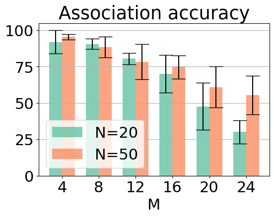
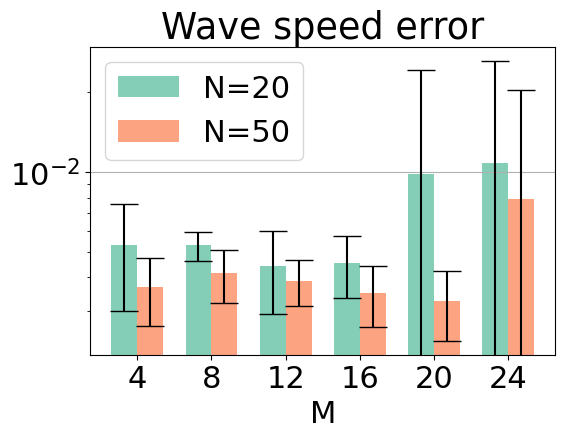
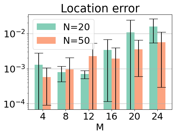
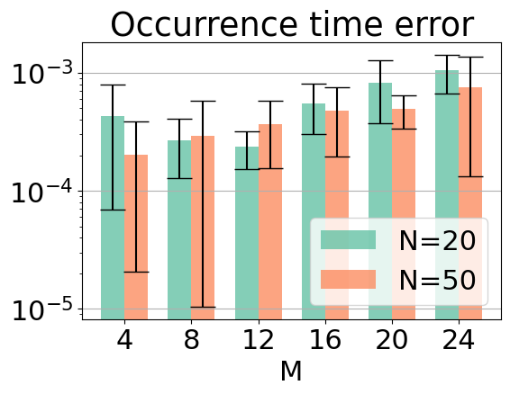
Figure 8: Evaluation of Harpa with varying number of stations $(N)$ and sources $(M)$. Left to right, the four panels illustrate the impact on (a) association accuracy, (b) relative wave speed error, (c) relative earthquake location error, and (d) relative earthquake occurrence time error. Bars show the mean of 10 independent runs; error bars indicate standard deviation. For efficiency we used a smaller and simpler dataset, with up to $2$ random fields compared to $3$ in other experiments and the latent dimension $L=4$ instead of $L=6$ (See Materials and method for the data generation protocol). The mean $\mathsf{CF}$ is $0.80$.

We constructed a dataset of synthetic wave speeds by superimposing realizations of a Gaussian random field onto a vertical gradient wave speed (details in Materials and method). This is a challenging setting for association which exhibits strong spatial variation and a large five-fold dynamic range of wave speeds, typically between 5 km/s and 25 km/s. The test wave speed in this experiment comes from the same distribution (it is not included in the training set). In Materials and method we also report results for a different distribution of wave speeds obtained as random Gaussian perturbations.

Fig. 6 shows results for a setting with $\mathsf{CF}=0.94$. The root-mean-squared error (RMSE) between the true and recovered wave speeds is is $0.78$ km/s; the pointwise error is everywhere below 2 km/s; the RMSE in earthquake spatial locations is $3.48$ km. This is achieved with wave speeds ranging from $5$ km/s to $25$ km/s within a $100$ km $\times$ $100$ km $\times$ $100$ km volume. As a result of this accurate recovery, the accuracy of the subsequent association is 91.3%. As we can see from the left panel in Fig. 6, Harpa achieves this high association accuracy in spite of the fact that the waves arrive at the different stations in completely different sequences and are packed close together in time; existing methods simply do not work in this regime. The only association errors made by Harpa are for the picks which are almost entirely overlapped and which are confused with their neighbors.

In Fig. 7 we test the performance of Harpa in handling a high number of simultaneous earthquake events. We perform association for 16 arrivals occurring in less than half the time in Fig. 6. We see that with 50 stations we can nonetheless obtain an accurate association, again with most of the confused arrivals being close in time. When the number of stations decreases to 20 the association accuracy deteriorates.

Interestingly, while additional stations and sources might initially cause confusion in arrival times and contribute to erroneous association, they enhance wave speed reconstruction. For example, in the top row in Fig. 7, even though the earthquake locations and wave speed are accurately recovered (with mean errors of $3.18$ km and $1.94$ km/s), the misassociations are inevitable due to completely overlapping arrivals. Increasing the number of stations and sources provides additional travel time information, ultimately benefitting wave speed reconstruction. More results for different numbers of stations and events are shown in Fig. 8.

Distorted and out-of-distribution wave speeds

Next, we study the robustness of the proposed method in situations where the true wave speed comes from a different distribution than the one used to train Harpa’s travel time neural field. In other words, the ground truth wave speed is markedly different from any wave speed seen by the autoencoder, both qualitatively and quantitatively.

In the “distortion” experiment (Fig. 9a), we use the same fixed wave speed $c_{0}$ used in the previous known wave speed experiment to learn travel time neural fields, while the true (test) wave speed is a linear interpolation between $c_{0}$ and another fixed wave speed $c_{1}$, $c^{*}=(1-p_{d})c_{0}+p_{d}c_{1}$; when $p_{d}=0$, there is no model distortion between training and deployment. In the “out of distribution” experiment (Fig. 9b), we use the travel time neural field for a wave speed distribution described in the previous unknown wave speed experiment. The true (test) wave speed is generated according to $c^{*}=(1-p_{o})c_{2}+p_{o}c_{0}$, where $c_{2}$ is a wave speed randomly sampled in-distribution and $c_{0}$ is the out-of-distribution perturbation. A large $p_{o}$ means that $c^{*}$ is far from the training wave speed distribution In either case we let $c_{0}$ be the SEG/EAGE 3-D overthrust model, qualitatively rather different from Gaussian random field samples $c_{1}$ and $c_{2}$.

We highlight that, compared with the fixed wave speed experiment in Fig. 9a, the generative model in Harpa makes the recovery much more robust. For small $\mathsf{CF}$, the association accuracy (orange heatmap) is still very high even though the test wave speed is far out of distribution. It is further worth noting that in cases where the arrival sequence from different events is similar at all stations (small $\mathsf{CF}$), accurate wave speed recovery and source localization are not necessary for a good association. This observation aligns with previous studies on the low-rate regime where fixed wave speed models which only vary in the depth coordinate yield good association performance.

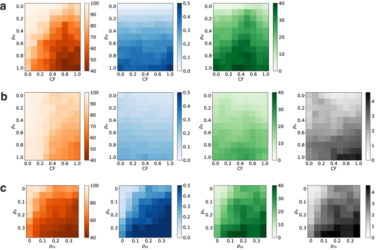
Figure 9: Robustness of Harpa under distortion and noise quantified by association accuracy $\mathsf{ACC}$ (orange), signal matching error $e_{l}$ in seconds (blue), earthquake location error in km (green) and mean wave speed reconstruction error in km/s (grey), as a function of (a) wave speed distortion ($p_{d}$) and the confusion factor $\mathsf{CF}$; (b) excursion from training distribution ($p_{o}$) and confusion factor $\mathsf{CF}$; (c) fraction of noisy ($p_{n}$) and missing ($p_{m}$) picks. All values are averages of 20 trials. In (c), the $\mathsf{ACC}$ and $e_{l}$ are determined by comparison with the original noiseless picks and the average $\mathsf{CF}$ is $0.80$; the setting in other panels is as in Fig. 8.

Spurious and missing picks

When working with real seismograms it may happen that some picks are missing, for example because a station is too far from the source. On the contrary, the peak picking algorithm may make spurious detections. We test the robustness of Harpa to these types of errors. In Fig. 9c, we arbitrarily eliminate a $p_{m}$ fraction of arrivals at each station and introduce an additional fraction $p_{n}$ of random picks. When $p_{n}>p_{m}$, the number of picks at each station is typically larger than the number of events we are searching for. On the contrary, when $p_{n}<p_{m}$, the number of picks at each station is typically smaller than the number of events we are searching for. We see in the figure that small-to-moderate ratios of noisy and missing picks do not significantly hurt the association accuracy (orange heat map in Fig. 9c) even when $\mathsf{CF}=0.80$.

Discussion

Existing association algorithms operate under the assumption that the wave speed is approximately known and are applied in low-rate settings where the order of arrivals of waves from the different events coincides at all stations  (?). A major challenge addressed by these methods is to sieve out spurious and missing arrivals which hamper association.

We explore a different regime where the arrivals are extremely dense in occurrence time, the ordinal number of arrivals at a station is a priori meaningless, and the wave speed is unknown. This regime is of great interest for earthquake monitoring but inaccessible to existing methods; see, for example, the density and mixing-up of arrivals that we successfully associate in Fig. 8, notwithstanding the unknown wave speed. The fact that we can still obtain accurate associations in situations of this complexity opens up new domains of application. Quoting from  (?), “a comprehensive study of microseismicity can provide a valuable description of the geological medium properties and earthquake related processes in the investigated crustal volumes, such as, for instance, the identification and geometrical characterization of active fault structures.”.

Indeed, taming microseismicity would allow us to monitor the changes in time of the elastic material properties. One case in point is monitoring sustainable energy production facilities  (?); another is understanding fault activity in earthquakes caused by “unconventional hydrocarbon development” (fracking); as Park and coauthors write  (?), “Microearthquake activity can illuminate otherwise unknown faults, particularly when events are detected down to low magnitudes and are located precisely.”

From a high-level perspective, there are two reasons that make our proof of concept, Harpa, work. The first is that we take an inverse problems perspective and approximately recover continuous unknowns by interpreting the observed data as a probability measure. Indeed, in situations of such complexity, it is unlikely that statistical filtering methods can work well without explicitly using some model of wave propagation. Since we still only obtain (coarse) approximations of the relevant parameters, we cannot claim to solve the full travel time tomography problem, but it is conceivable that the resulting association and the approximate locations and wave speeds could be used as a warm start for a linearized or iterative method  (?).

The second reason is that we leverage a body of theoretical and engineering developments from deep learning: efficient optimal transport routines, neural fields, automatic differentiation, generative models, stochastic optimization and sampling, are all essential components of Harpa.

Computer experiments show that Harpa is robust to deviations of wave speed models from the distribution used in training and to noisy arrival picks. A fully practical field deployment, however, requires additional work on robustness to spurious and missing picks which may be achieved through a judicious use of sparse unbalanced optimal transport. Another exciting possibility is to use multiple temporal windows instead of a single one and thus effectively work with a very large number of events. This is straightforward in principle but the current bottleneck is computational efficiency. Faster optimization algorithms would open up the possibility to work with general rather than low-dimensional wave speed models and ultimately perform ab initio nonlinear travel time tomography with unknown sources.

Materials and methods

Wave speed autoencoders

We discretize the wave speed into a 32 $\times$ 32 $\times$ 32 cube, i.e., $c\in\mathbb{R}^{32\times 32\times 32}$, and use these cubic images to train a standard CNN autoencoder in pytorch. Due to the low-dimensional structure of the dataset, the autoencoder exhibits strong generalization when an appropriate dimension of the latent code $z\in\mathbb{R}^{L}$ is selected. A large $L$ yields an autoencoder which accurately represents the wave speeds but also leads to slow SGLD inference. In our experiments we tested values of $L$ between 3 and 6. The generalization performance of the autoencoder is illustrated in Fig. S4.

The encoder comprises three 3D convolutional layers with a kernel size of $3^{3}$, a stride of 2, and padding of 1, each followed by a ReLU activation function. A subsequent linear layer generates the latent code $z$. Batch normalization is implemented between each layer. The decoder’s architecture mirrors that of the encoder.

Training the travel time neural field

We compute the travel times from the receivers to to all 32 $\times$ 32 $\times$ 32 grid points for the aforementioned 10000 wave speeds using the fast marching method implemented in the scikit-fmm package.

We create a $(L+3)$-dimensional feature vector for each grid point by concatenating its coordinate and the corresponding wave speed latent code, which are all scaled in $[0,1]$ as the input to the neural field. We use a SIREN implicit network, a multilayer perceptron (MLP) with periodic activation functions  (?). The trained SIREN model not only provides accurate predictions of the travel time at the grid points but also immediately yields an interpolation at arbitrary continuous coordinates. The scaling constant $w_{0}$ in the sinusoidal activation function is important and depends on the grid scaling; we used $w_{0}=15$.

Optimization

We use the Python Optimal Transport (POT) package to compute the Wasserstein-2 distance, with $p=2$. We adopt the RMSProp-preconditioned version of the SGLD  (?). Both the learning rate $(lr)$ and the noise factor $(\epsilon)$ are selected from $\{10^{-2},10^{-3},5\times 10^{-3},10^{-4}\}$. The convergence speed depends on the choice of hyperparameters. To manage the exploration-exploitation trade-off, we reduce the learning rate $(lr)$ to one-tenth of its original value once the loss decreases below a threshold $l^{*}$ which is selected from $\{10^{-2},10^{-3},10^{-4},10^{-6}\}$. To speed up training, we implement an epoch threshold. If the loss fails to decrease below $l^{*}$ before reaching this threshold, we reset all the parameters and restart the training process. We set the maximum number of trials to 10. When $\tau_{\max}$ is very large or $\mathsf{CF}$ is close to $0$, pre-training $\tau$ helps achieve faster convergence.

Comparison between SGD and SGLD

Here we show that due to non-convexity naive (stochastic) gradient descent converges to poor local minima, and that the issue is mitigated by SGLD. We compare SGD and SGLD on the fixed wave speed datasets described in Experiments. To visualize the optimization trajectory, we set the learning rate to $0.005$ and $\epsilon=0.0005$ (cf. (12)) for all epochs. Setting $\epsilon=0$ reduces SGLD to SGD; the corresponding performance is reported in the second row in Fig. S1. A visual comparison of the trajectories of the source estimates during optimization (Fig. S1, right) clearly shows that unlike SGD, SGLD easily escapes bad local minima.

Gaussian random field dataset

In Figures 6, 7, and 8, the wave speeds are samples from the Gaussian random field dataset. To generate this low-dimensional wave speed dataset, we first created 20 three-dimensional Gaussian random fields as basis patterns in which the correlation is determined by the scale-invariant power spectrum $P(k)\sim k^{-\alpha/2}$  (?, ?). We use $\alpha=2.5$ in our experiments and rescale the pattern amplitudes to lie between $0$ km/s and $15$ km/s; representative samples are shown in Fig. S3. For each sample, we randomly select up to 3 patterns and then add the selected patterns to a background wave speed (Fig. S2) with weights drawn uniform at random in $[-1,1]$. All wave speeds are clipped between $5$ km/s and $25$ km/s. In Fig. S4 we show that this dataset is effectively modeled by a 3D convolutional autoencoder.

Gaussian random perturbation dataset

In Fig. S6 we report results for a different dataset in which we add between one and three random Gaussian perturbations to the background wave speed. These perturbations are defined as

$$\Delta c(x,y,z)=A\exp\left(-\frac{1}{2\sigma_{x}^{2}}(x-x_{0})^{2}-\frac{1}{2\sigma_{y}^{2}}(y-y_{0})^{2}-\frac{1}{2\sigma_{z}^{2}}(z-z_{0})^{2}\right),$$

where $A$ is drawn uniformly at random from $[-25,25]$, $x_{0},y_{0},z_{0}$ uniformly at random from $[0,100]$ and $\sigma_{x},\sigma_{y},\sigma_{z}$ uniformly at random from $[10,50]$; samples are shown Fig. S5.

A Wasserstein misfit for unbalanced arrivals matching

We denote the cardinality of a finite set $S$ by $|S|$ and let $\rho_{S}$ be the uniform probability measure over its elements,

$$\rho_{S}=\frac{1}{|S|}\sum_{s\in S}\mathbbm{1}_{s}.$$

We now consider two sets (of arrival times) $A$ and $B$ of possibly different cardinality. Without loss of generality, we assume $|A|\leq|B|$. We define a Wasserstein-like mismatch between these arrival sets as

$$\widehat{w}_{p}(A,B)=\min_{\widetilde{B}\subseteq B,\leavevmode\nobreak\ |\widetilde{B}|=|A|}w_{p}(\rho_{A},\rho_{\widetilde{B}})$$

with $w_{p}$ defined in Equation (9). This mismatch can be optimized by sparsity-constrained optimal transport  (?). In fact, in the 1D case it coincides with the loss of the unbalanced linear assignment problem

$$\overline{w}_{p}(A,B)=\min_{T\in\mathcal{T}_{|A|,|B|}}\tfrac{1}{|A|}\langle T,C\rangle,$$

where (arbitrarily vectorizing the elements of $A$ and $B$ as $a=(a_{1},\ldots,a_{|A|})$ and $b=(b_{1},\ldots,b_{|B|})$) we used

$$\mathcal{T}_{|A|,|B|} :=\left\{T\in\{0,1\}^{|A|\times|B|}:T\mathbf{1}_{|B|}=\mathbf{1}_{|A|},\leavevmode\nobreak\ T^{\top}\mathbf{1}_{|B|}\leq\mathbf{1}_{|A|}\right\},$$ (15)

$$C_{ij} :=|a_{i}-b_{j}|^{p}.$$

Here $\langle\cdot,\cdot\rangle$ denotes the Frobenius inner product and $T$ the discrete transportation matrix. The all-ones vector of length $K$ is denoted $\mathbf{1}_{K}$. For vectors $x,y\in\mathbb{R}^{K}$, the notation $x\leq y$ indicates that the inequality holds for all entries.

Supplementary materials

Figs. S1 to S6

Supplementary Materials

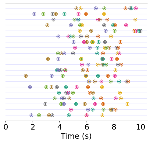
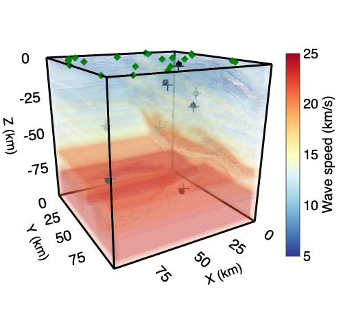
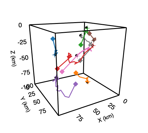
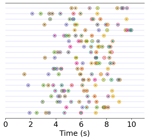
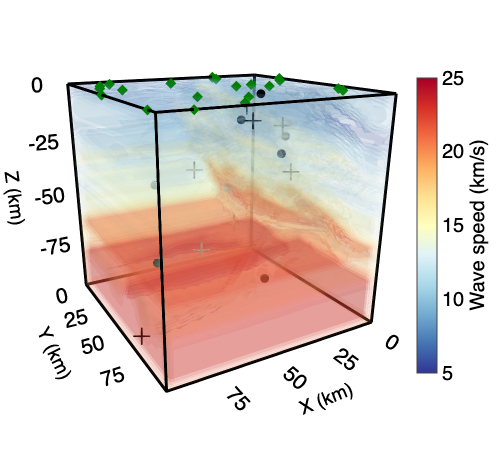
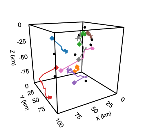
Figure S1: Association results for $8$ sources, $20$ stations and $\mathsf{CF}=0.85$ with SEG/EAGE 3-D overthrust model as the known wave speed. Top row (SGLD): $\mathsf{ACC}=92.5\%$, $e_{l}=0.02s$. Bottom row (SGD): $\mathsf{ACC}=37.5\%$, $e_{l}=0.59s$. Symbols and encoding are as in Fig. 5; the right plot illustrates the source trajectories in the first 30 optimization epochs.

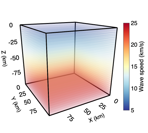
Figure S2: Background wave speed

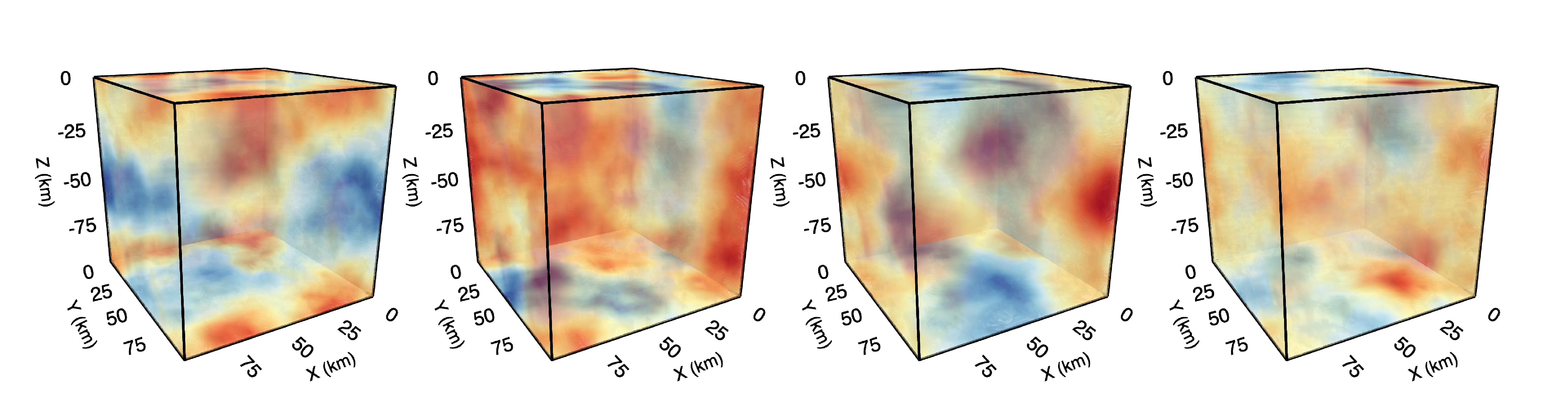
Figure S3: Four samples of the 3D Gaussian random fields with $\alpha=2.5$.

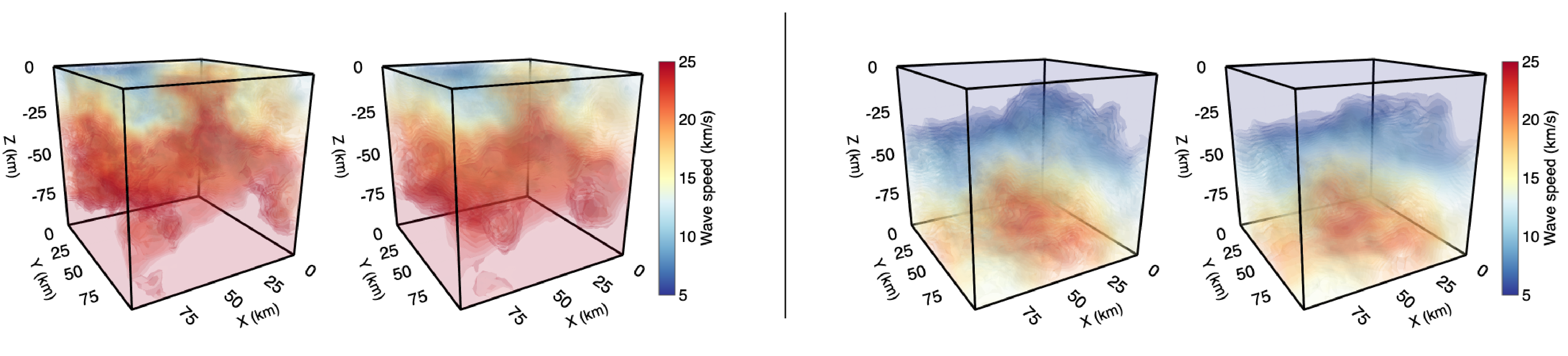
Figure S4: A comparison between two test wave speeds unseen at training time and the corresponding outputs from an auto-encoder with $L=6$.

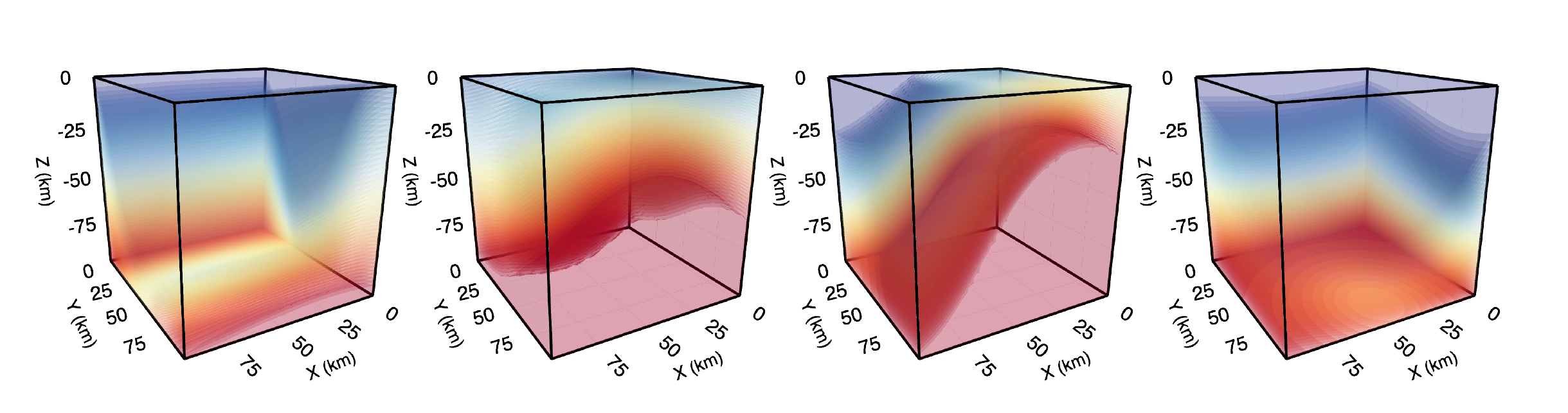
Figure S5: Four samples of wave speeds from the Gaussian perturbation dataset.

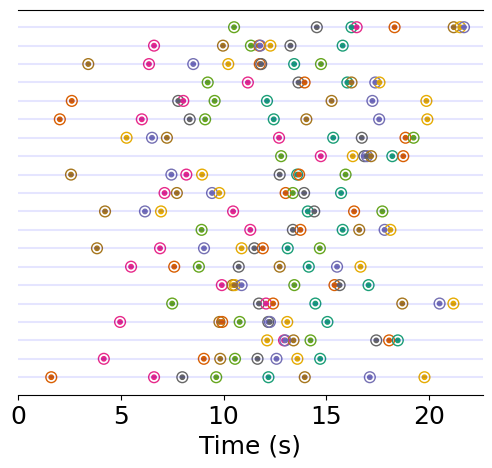
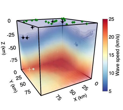
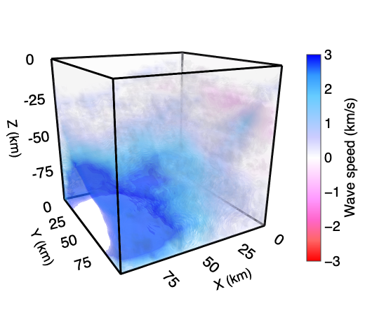
Figure S6: Association results for $8$ sources, $20$ stations and $\mathsf{CF}=0.79$ on Gaussian perturbation dataset. Harpa achieves $\mathsf{ACC}=96.3\%$ and $e_{l}=0.02$ s. Symbols and encoding are as in Fig. 6

References

- 1. Z. E. Ross, M.-A. Meier, E. Hauksson, T. H. Heaton, Generalized seismic phase detection with deep learning. Bulletin of the Seismological Society of America 108, 2894–2901 (2018).
- 2. S. M. Mousavi, W. L. Ellsworth, W. Zhu, L. Y. Chuang, G. C. Beroza, Earthquake transformer—an attentive deep-learning model for simultaneous earthquake detection and phase picking. Nature communications 11, 3952 (2020).
- 3. W. Zhu, G. C. Beroza, Phasenet: A deep-neural-network-based seismic arrival-time picking method. Geophysical Journal International 216, 261–273 (2019).
- 4. V. Grechka, W. M. Heigl, Microseismic monitoring (Society of Exploration Geophysicists Tulsa, 2017).
- 5. W. Zhu, I. W. McBrearty, S. M. Mousavi, W. L. Ellsworth, G. C. Beroza, Earthquake phase association using a Bayesian Gaussian mixture model. Journal of Geophysical Research: Solid Earth 127, e2021JB023249 (2022).
- 6. H. Sato, M. C. Fehler, T. Maeda, Seismic wave propagation and scattering in the heterogeneous earth (Springer Science & Business Media, 2012).
- 7. M. V. de Hoop, J. Ilmavirta, M. Lassas, T. Saksala, Stable reconstruction of simple Riemannian manifolds from unknown interior sources. arXiv preprint arXiv:2102.11799 (2021).
- 8. V. Sitzmann, J. Martel, A. Bergman, D. Lindell, G. Wetzstein, Implicit neural representations with periodic activation functions. Advances in Neural Information Processing Systems 33, 7462–7473 (2020).
- 9. B. Mildenhall, P. P. Srinivasan, M. Tancik, J. T. Barron, R. Ramamoorthi, R. Ng, Nerf: Representing scenes as neural radiance fields for view synthesis. Communications of the ACM 65, 99–106 (2021).
- 10. Y. Xie, T. Takikawa, S. Saito, O. Litany, S. Yan, N. Khan, F. Tombari, J. Tompkin, V. Sitzmann, S. Sridhar, Computer Graphics Forum (Wiley Online Library, 2022), vol. 41, pp. 641–676.
- 11. M. Welling, Y. W. Teh, Proceedings of the 28th International Conference on Machine Learning (2011), pp. 681–688.
- 12. R. Burkard, M. Dell’Amico, S. Martello, Assignment problems: revised reprint (SIAM, 2012).
- 13. T. C. Koopmans, M. Beckmann, Assignment problems and the location of economic activities. Econometrica: Journal of the Econometric Society pp. 53–76 (1957).
- 14. P. M. Pardalos, H. Wolkowicz, et al., Quadratic Assignment and Related Problems: DIMACS Workshop, May 20-21, 1993, vol. 16 (American Mathematical Soc., 1994).
- 15. R. K. Ahuja, J. B. Orlin, A. Tiwari, A greedy genetic algorithm for the quadratic assignment problem. Computers & Operations Research 27, 917–934 (2000).
- 16. U. Benlic, J.-K. Hao, Breakout local search for the quadratic assignment problem. Applied Mathematics and Computation 219, 4800–4815 (2013).
- 17. O. Vinyals, M. Fortunato, N. Jaitly, Pointer networks. Advances in neural information processing systems 28 (2015).
- 18. Z. Li, Q. Chen, V. Koltun, Combinatorial optimization with graph convolutional networks and guided tree search. Advances in Neural Information Processing Systems 31 (2018).
- 19. A. Nowak, S. Villar, A. S. Bandeira, J. Bruna, 2018 IEEE Data Science Workshop (DSW) (IEEE, 2018), pp. 1–5.
- 20. C. A. Floudas, Nonlinear and mixed-integer optimization: fundamentals and applications (Oxford University Press, 1995).
- 21. E. L. Geist, T. Parsons, Determining on-fault earthquake magnitude distributions from integer programming. Computers & Geosciences 111, 244–259 (2018).
- 22. P. Belotti, C. Kirches, S. Leyffer, J. Linderoth, J. Luedtke, A. Mahajan, Mixed-integer nonlinear optimization. Acta Numerica 22, 1–131 (2013).
- 23. J. Sun, Z. Xue, T. Zhu, S. Fomel, N. Nakata, SEG International Exposition and Annual Meeting (SEG, 2016), pp. SEG–2016.
- 24. B. Witten, J. Shragge, Image-domain velocity inversion and event location for microseismic monitoring. Geophysics 82, KS71–KS83 (2017).
- 25. C. Song, T. Alkhalifah, Z. Wu, Microseismic event estimation and velocity analysis based on a source-focusing function. Geophysics 84, KS85–KS94 (2019).
- 26. J. Jansky, V. Plicka, L. Eisner, Feasibility of joint 1d velocity model and event location inversion by the neighbourhood algorithm. Geophysical Prospecting 58, 229–234 (2010).
- 27. Z. Zhang, J. W. Rector, M. J. Nava, Simultaneous inversion of multiple microseismic data for event locations and velocity model with Bayesian inference. Geophysics 82, KS27–KS39 (2017).
- 28. I. Dokmanić, R. Parhizkar, A. Walther, Y. M. Lu, M. Vetterli, Acoustic echoes reveal room shape. Proceedings of the National Academy of Sciences 110, 12186–12191 (2013).
- 29. S. Huang, I. Dokmanić, Reconstructing point sets from distance distributions. IEEE Transactions on Signal Processing 69, 1811–1827 (2021).
- 30. L. Zhu, Z. Peng, J. McClellan, C. Li, D. Yao, Z. Li, L. Fang, Deep learning for seismic phase detection and picking in the aftershock zone of 2008 mw7. 9 wenchuan earthquake. Physics of the Earth and Planetary Interiors 293, 106261 (2019).
- 31. Z. E. Ross, Y. Yue, M.-A. Meier, E. Hauksson, T. H. Heaton, Phaselink: A deep learning approach to seismic phase association. Journal of Geophysical Research: Solid Earth 124, 856–869 (2019).
- 32. Z. E. Ross, W. Zhu, K. Azizzadenesheli, Neural mixture model association of seismic phases. arXiv preprint arXiv:2301.02597 (2023).
- 33. I. W. McBrearty, J. Gomberg, A. A. Delorey, P. A. Johnson, Earthquake arrival association with backprojection and graph theory. Bulletin of the Seismological Society of America 109, 2510–2531 (2019).
- 34. I. W. McBrearty, G. C. Beroza, Earthquake phase association with graph neural networks. Bulletin of the Seismological Society of America (2023).
- 35. M. Shahnas, D. Yuen, R. Pysklywec, Inverse problems in geodynamics using machine learning algorithms. Journal of Geophysical Research: Solid Earth 123, 296–310 (2018).
- 36. P. Mora, G. Morra, D. A. Yuen, Models of plate tectonics with the Lattice Boltzmann Method. Artificial Intelligence in Geosciences 4, 47–58 (2023).
- 37. F. Lehmann, F. Gatti, M. Bertin, D. Clouteau, Machine learning opportunities to conduct high-fidelity earthquake simulations in multi-scale heterogeneous geology. Frontiers in Earth Science 10, 1029160 (2022).
- 38. M. Liu, M. Zhang, W. Zhu, W. L. Ellsworth, H. Li, Rapid characterization of the July 2019 Ridgecrest, California, earthquake sequence from raw seismic data using machine-learning phase picker. Geophysical Research Letters 47, e2019GL086189 (2020).
- 39. A. Zang, V. Oye, P. Jousset, N. Deichmann, R. Gritto, A. McGarr, E. Majer, D. Bruhn, Analysis of induced seismicity in geothermal reservoirs–an overview. Geothermics 52, 6–21 (2014).
- 40. S. Glubokovskikh, C. S. Sherman, J. P. Morris, D. L. Alumbaugh, Transforming microseismic clouds into near real-time visualization of the growing hydraulic fracture. Geophysical Journal International p. ggad248 (2023).
- 41. Y.-A. Ma, Y. Chen, C. Jin, N. Flammarion, M. I. Jordan, Sampling can be faster than optimization. Proceedings of the National Academy of Sciences 116, 20881–20885 (2019).
- 42. P. Xu, J. Chen, D. Zou, Q. Gu, Global convergence of Langevin dynamics based algorithms for nonconvex optimization. Advances in Neural Information Processing Systems 31 (2018).
- 43. F. Aminzadeh, P. Weimer, T. Davis, 3-d salt and overthrust seismic models. Studies in Geology 42, 247–256 (1996).
- 44. M. G. Kendall, A new measure of rank correlation. Biometrika 30, 81–93 (1938).
- 45. Z. E. Ross, B. Idini, Z. Jia, O. L. Stephenson, M. Zhong, X. Wang, Z. Zhan, M. Simons, E. J. Fielding, S.-H. Yun, E. Hauksson, A. W. Moore, Z. Liu, J. Jung, Hierarchical interlocked orthogonal faulting in the 2019 Ridgecrest earthquake sequence. Science 366, 346–351 (2019).
- 46. G. M. Adinolfi, G. De Landro, M. Picozzi, F. Carotenuto, A. Caruso, S. Nazeri, S. Colombelli, S. Tarantino, T. Muzellec, A. Emolo, e. al., Comprehensive study of micro-seismicity by using an automatic monitoring platform. Frontiers in Earth Science 11, 1073684 (2023).
- 47. F. Grigoli, J. F. Clinton, T. Diehl, P. Kaestli, L. Scarabello, T. Agustsdottir, S. Kristjansdottir, R. Magnusson, C. J. Bean, M. Broccardo, e. al., Monitoring microseismicity of the Hengill Geothermal Field in Iceland. Scientific Data 9, 220 (2022).
- 48. Y. Park, G. C. Beroza, W. L. Ellsworth, Basement fault activation before larger earthquakes in oklahoma and kansas. The Seismic Record 2, 197–206 (2022).
- 49. H. Fang, R. D. Van Der Hilst, M. V. de Hoop, K. Kothari, S. Gupta, I. Dokmanić, Parsimonious seismic tomography with Poisson Voronoi projections: methodology and validation. Seismological Research Letters 91, 343–355 (2020).
- 50. C. Li, C. Chen, D. Carlson, L. Carin, Proceedings of the AAAI Conference on Artificial Intelligence (2016), vol. 30.
- 51. J. M. Bardeen, J. Bond, N. Kaiser, A. Szalay, The statistics of peaks of Gaussian random fields. Astrophysical Journal, Part 1 (ISSN 0004-637X), vol. 304, May 1, 1986, p. 15-61. SERC-supported research. 304, 15–61 (1986).
- 52. J. Dubinski, R. Carlberg, The structure of cold dark matter halos. Astrophysical Journal, Part 1 (ISSN 0004-637X), vol. 378, Sept. 10, 1991, p. 496-503. 378, 496–503 (1991).
- 53. T. Liu, J. Puigcerver, M. Blondel, International Conference on Learning Representations (2023).
Acknowledgments
Funding: C.S. and I.D. are supported by were supported by the European Research Council (ERC) Starting Grant 852821—SWING. M.V.d.H. is supported by the Simons Foundation under the MATH+X program, and Department of Energy, grant DE-SC0020345. Author contributions: C.S., M.V.d.H. and I.D. designed research, analyzed data, and wrote the paper. C.S. performed experiments. Competing interests: The authors declare that they have no competing interests. Data and materials availability: All data needed to evaluate the conclusions in the paper are present in the paper and/or the Supplementary Materials. Code at https://github.com/DaDaCheng/phase_association.