Photon and dilepton emission anisotropy for magnetized quark-gluon plasma

Abstract

We study the higher-order anisotropy coefficients $v_{4}$ and $v_{6}$ in the photon and dilepton emission from a hot magnetized quark-gluon plasma. Together with the earlier predictions for $v_{2}$, these results show a distinctive pattern of the anisotropy coefficients in several kinematic regimes. In the case of photon emission, nonzero coefficients $v_{n}$ (with even $n$) have opposite signs at small and large values of the transverse momentum (i.e., $k_{T}\lesssim\sqrt{|eB|}$ and $k_{T}\gtrsim\sqrt{|eB|}$, respectively). Additionally, the $v_{n}$ signs alternate with increasing $n$, and their approximate values decrease as $1/n^{2}$ in magnitude. The anisotropy of dilepton emission is well-pronounced only at large transverse momenta and small invariant masses (i.e., when $k_{T}\gtrsim\sqrt{|eB|}$ and $M\lesssim\sqrt{|eB|}$). The corresponding $v_{4}$ and $v_{6}$ coefficients are of the same magnitude and show a similar sign-alternative pattern with increasing $n$ as in the photon emission.

I Introduction

Quark-gluon plasma (QGP) is a state of extremely hot matter made of deconfined quarks and gluons that carry non-Abelian color charges Yagi et al. (2005); Rischke (2004); Shuryak (2017). The existence of such a plasma state stems from the asymptotic freedom in quantum chromodynamics (QCD) Gross and Wilczek (1973); Politzer (1973). QGP was present naturally in the early Universe about a microsecond after the Big Bang. It can also be produced in heavy-ion collisions at the Relativistic Heavy Ion Collider (RHIC) in Brookhaven and the Large Hadron Collider (LHC) at CERN. The corresponding “Little Bang” experiments allow one to study the fundamental properties of QGP Bzdak et al. (2020).

Despite small sizes and short interaction times in relativistic collisions, experimental data provide a strong evidence that the QGP forms a strongly interacting viscous liquid Back et al. (2005); Adcox et al. (2005); Adams et al. (2005). The flow measurements, quantified by the anisotropy coefficients $v_{n}$, support the scenario of QGP evolving hydrodynamically for a considerable fraction of its lifetime Heinz and Snellings (2013). Theoretical models also indicate that the plasma has low viscosity Bernhard et al. (2019), consistent with a strongly interacting regime.

The dynamics responsible for the QGP production in heavy-ion collisions are complicated and only partially understood. One of the aspects in dire need of better understanding is the possible generation and evolution of background magnetic fields in noncentral collisions. Theoretical studies suggest that the initial magnetic field $B$ could be of the order of $m_{\pi}^{2}/e\approx 3\times 10^{18}~{}G$ Skokov et al. (2009); Voronyuk et al. (2011); Deng and Huang (2012); Bloczynski et al. (2013); Tuchin (2016); Guo et al. (2020). Such an incredibly strong field could modify the thermodynamic and transport properties of QGP, trigger the chiral anomalous effects (CME) Fukushima et al. (2008); Kharzeev and Zhitnitsky (2007); Kharzeev et al. (2008), and ultimately affect numerous observables. For reviews, see Refs. Tuchin (2013a); Kharzeev et al. (2016); Huang (2016); Miransky and Shovkovy (2015).

To verify whether the QGP in noncentral collisions is magnetized and to estimate the strength of the magnetic field, one can try scrutinizing the most promising electromagnetic observables. It is reasonable to start by analyzing the photon Yee (2013); Tuchin (2015); Zakharov (2016) and dilepton emission rates Tuchin (2013b). Firstly, the magnetic field affects the corresponding rates already at leading order in coupling. Secondly, the photons and dileptons are clean probes of the QGP at early times. Indeed, owing to their long mean-free path, they do not suffer much from rescattering in a small volume of the plasma.

The heavy-ion experiments reveal that the direct photons have a sizable elliptic flow, quantified by a large ellipticity coefficient $v_{2}$ Adare et al. (2012, 2016); Acharya et al. (2019). Their flow appears to be comparable to that of hadrons, which is truly surprising. Unlike hadrons, the direct photons are emitted at early times of QGP when collective flow may not have had the chance to form yet. This is known as the “direct photon” puzzle. Many theoretical studies tried to address it Chatterjee et al. (2006); Schenke and Strickland (2007); Chatterjee and Srivastava (2009); van Hees et al. (2011); Linnyk et al. (2014); Gale et al. (2015); Muller et al. (2014); van Hees et al. (2015); Monnai (2014); Dion et al. (2011); Liu and Liu (2014); Vujanovic et al. (2014); McLerran and Schenke (2014, 2016); Gelis et al. (2004); Hidaka et al. (2015); Linnyk et al. (2016); Vovchenko et al. (2016); Koide and Kodama (2016); Turbide et al. (2006); Tuchin (2013c); Basar et al. (2012). In our detailed studies of the differential rates in Refs. Wang et al. (2020); Wang and Shovkovy (2021a), in particular, we argued that a large positive $v_{2}$ of the direct photons may be explained by the presence of a strong background magnetic field in the QGP.

The dilepton emission is another complementary probe of the QGP. Since their spectra are not affected by the blue shift of the expanding medium, dileptons can serve as an excellent thermometer of the QGP Rapp and van Hees (2016). On the other hand, the dilepton rate should be affected by the magnetic field Sadooghi and Taghinavaz (2017); Bandyopadhyay et al. (2016); Bandyopadhyay and Mallik (2017); Ghosh and Chandra (2018); Islam et al. (2019); Das et al. (2019); Ghosh et al. (2020); Chaudhuri et al. (2021); Das et al. (2022). Moreover, as we demonstrated in the earlier study Wang and Shovkovy (2022), the dilepton emission is characterized by a sizable ellipticity at small values of the invariant mass ($M\lesssim\sqrt{|eB|}$). In the same kinematic region, the rate is also strongly enhanced. It is fair to mention that the corresponding theoretical claims may be hard to verify systematically in current experiments.

Here we extend the previous studies by showing that the presence of a strong magnetic field in the QGP should be encoded not only in $v_{2}$ but also in high-order anisotropy coefficients. By using the same theoretical framework as in Refs. Wang et al. (2020); Wang and Shovkovy (2021a, 2022), here we obtain detailed theoretical predictions for the higher-order anisotropy coefficients $v_{4}$ and $v_{6}$. Similarly to $v_{2}$, they show nontrivial dependence on the kinematic parameters. We argue that the future detailed measurements of the photon and dilepton anisotropy coefficients could provide a distinctive fingerprint for verifying the presence of the background magnetic field in the plasma produced by noncentral heavy-ion collisions.

This paper is organized as follows. In Sec. II, we introduce the key definitions and model assumptions in our study of the photon and dilepton emission from a hot magnetized QGP. The numerical results for higher-order anisotropy coefficients $v_{4}$ and $v_{6}$ are obtained and discussed in Sec. III. The summary of the main findings and conclusions are given in Sec. IV. In Appendix A, we quote the expression for the imaginary part of the Lorentz-contracted polarization tensor, which is needed for calculating the photon and dilepton rates.

II Model

Here we make the same model assumptions about the QGP as in Refs. Wang et al. (2020); Wang and Shovkovy (2021a, 2022). We consider a plasma made of the lightest up and down quarks. While the quantitive results may change slightly with the inclusion of the strange quarks, all qualitative results are to remain the same. For simplicity, we also assume that the masses of the up and down quarks are equal, i.e., $m_{u}=m_{d}=m$. It is an excellent approximation for the QGP with a temperature of several hundred megaelectronvolts.

Having heavy-ion physics in mind, we will consider the plasma at midrapidity. By assumption, the magnetic field points along the $z$-axis in the local rest frame. The field is perpendicular to the reaction plane (i.e., $x$-$y$ plane), and the beam direction is along the $x$-axis. The photon and dilepton emission setups are illustrated schematically in the two panels of Fig. 1.

In the case of photon emission, the corresponding four-momentum $k^{\mu}=(\Omega,\mathbf{k})$ satisfies the on-shell condition $k^{2}\equiv k_{\mu}k^{\mu}=0$. In the dilepton case, on the other hand, the photon $\gamma^{*}$ is virtual. Its momentum describes a lepton pair and satisfies a different on-shell condition, i.e., $k^{2}=M^{2}$, where $M$ is the dilepton invariant mass. Note that $k_{x}=0$ at midrapidity (i.e., $\frac{1}{2}\ln\frac{\Omega+k_{x}}{\Omega-k_{x}}=0$). The nonzero transverse components of the momentum are

$$k_{y}=k_{T}\cos(\phi),\qquad k_{z}=k_{T}\sin(\phi),$$ (1)

where $k_{T}=\sqrt{k_{y}^{2}+k_{z}^{2}}$ is the magnitude of the transverse momentum and $\phi$ is the azimuthal angle measured from the reaction plane. (The transverse component of the momentum $k_{T}$, which is perpendicular to the beam, should not be confused with $k_{\perp}=\sqrt{k_{x}^{2}+k_{y}^{2}}$, which is the component perpendicular to the magnetic field.)

II.1 Photon emission rate and its anisotropy

The thermal photon production rate from the QGP can be conveniently expressed in terms of the imaginary part of the retarded polarization tensor as follows Kapusta and Gale (2011):

$$k^{0}\frac{d^{3}R}{dk_{x}dk_{y}dk_{z}}=\frac{d^{3}R}{k_{T}dk_{T}d\phi dy}=-\frac{1}{(2\pi)^{3}}\frac{\mbox{Im}\left[\Pi^{\mu}_{R,\mu}\left(\Omega,\mathbf{k}\right)\right]}{\exp\left(\frac{\Omega}{T}\right)-1}.$$ (2)

The latter expression has the same form in QGP with and without a background field. However, a nonzero magnetic field can strongly affect the photon polarization tensor and, in turn, modify the photon emission rate. Below we will utilize the leading-order one-loop expression for $\mbox{Im}\left[\Pi^{\mu}_{R,\mu}\left(\Omega,\mathbf{k}\right)\right]$ derived in Refs. Wang et al. (2020); Wang and Shovkovy (2021b, 2022) by using the Landau-level representation for quarks. For convenience, we also quote the corresponding result in Appendix A.

When the differential rate (2) is known, the anisotropy coefficients $v_{n}$ can be evaluated as follows:

$$v_{n}(k_{T})=\frac{1}{\mathcal{R}_{0}}\int_{0}^{2\pi}\frac{d^{3}R}{k_{T}dk_{T}d\phi dy}\cos(n\phi)d\phi,$$ (3)

where the normalization factor is determined by integrating the emission rate over the azimuthal angle $\phi$, i.e.,

$$\mathcal{R}_{0}=\frac{d^{2}R}{k_{T}dk_{T}dy}=\int_{0}^{2\pi}\frac{d^{3}R}{k_{T}dk_{T}dyd\phi}d\phi.$$ (4)

We will use the definition in Eq. (3) to quantify the anisotropy of the photon emission from a hot magnetized QGP in Sec. III.

It is appropriate to comment on the approximation used here. When utilizing the one-loop polarization tensor in Eq. (2), one accounts for the following three leading-order processes: (i) the quark splitting ($q\rightarrow q+\gamma$), (ii) the antiquark splitting ($\bar{q}\rightarrow\bar{q}+\gamma$), and (iii) the quark-antiquark annihilation ($q+\bar{q}\rightarrow\gamma$) Wang et al. (2020); Wang and Shovkovy (2021b). Their contributions to the rate are of order $\alpha$, where $\alpha\equiv e^{2}/(4\pi)=1/137$ is the fine structure constant. Recall that the same processes are forbidden by energy-momentum conservation in the absence of the magnetic field. Instead, leading contributions at $B=0$ come from the gluon-mediated $2\to 2$ processes $q+g\rightarrow q+\gamma$, $\bar{q}+g\rightarrow\bar{q}+\gamma$, and $q+\bar{q}\rightarrow g+\gamma$, where $g$ represents a gluon Kapusta et al. (1991); Baier et al. (1992); Aurenche et al. (1998); Steffen and Thoma (2001); Arnold et al. (2001a, b); Ghiglieri et al. (2013). Formally, they are suppressed by an extra power of $\alpha_{s}$, where $\alpha_{s}\equiv g_{s}^{2}/(4\pi)$ is the QCD strong coupling constant.

Unfortunately, the gluon-mediated $2\to 2$ processes have not been analyzed in a magnetic field. Thus, it is unclear how the relative contributions of the leading and subleading diagrams vary when one goes continuously from the zero-field to the strong-field limit. Here we will assume that the magnetic field is sufficiently strong for the leading-order contributions $\sim\alpha$ (from the $1\to 2$ and $2\to 1$ processes) to dominate the anisotropy coefficients. It can be true even in some cases when the subleading contributions $\sim\alpha\alpha_{s}$ (from the gluon-mediated $2\to 2$ processes) dominate the rates. With the current knowledge, however, we cannot establish a rigorous range of validity for the approximation used. It is an important issue and should be addressed in detail in future studies.

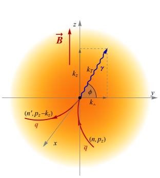
Figure 1: Schematic illustrations of the photon (panel a) and dilepton (panel b) emission from a magnetized plasma at midrapidity. The transverse momenta $k_{T}$ of the on-shell (in panel a) and virtual (in panel b) photons lie in the $y$-$z$ plane. The azimuthal angle $\phi$ is measured from the reaction plane, which coincides with the $x$-$y$ plane. The lepton momenta outside the magnetized plasma are $q_{1}$ and $q_{2}$ (panel b).

II.2 Dilepton emission rate and its anisotropy

Similarly to the photon emission, the differential dilepton production rate can be expressed in terms of the imaginary part of the photon polarization tensor, i.e.,

$$\frac{dR_{l\bar{l}}}{d^{4}k}=\frac{\alpha}{12\pi^{4}}\frac{n_{B}\left(\Omega\right)}{M^{2}}\mbox{Im}\left[\Pi^{\mu}_{R,\mu}\left(\Omega,\mathbf{k}\right)\right],$$ (5)

where $n_{B}(\Omega)=(e^{\Omega/T}-1)^{-1}$ is the Bose-Einstein distribution function. Here we neglected the nonzero lepton masses and took into account that $k^{2}\equiv\Omega^{2}-k_{\perp}^{2}-k_{z}^{2}=M^{2}$. Note that $\Omega=\sqrt{M^{2}+k_{\perp}^{2}+k_{z}^{2}}$ and $d^{4}K=MdMk_{T}dk_{T}dyd\phi$.

To quantify the anisotropy of dilepton emission in Sec. III, we will use the Fourier coefficients similar to those in Eq. (3), i.e.,

$$v_{n}(M,k_{T})=\frac{\int_{0}^{2\pi}d\phi\cos(n\phi)\left(dR_{l\bar{l}}/d^{4}k\right)}{\int_{0}^{2\pi}d\phi\left(dR_{l\bar{l}}/d^{4}k\right)}.$$ (6)

It is instructive to emphasize that the approximation for the dilepton rate in Eq. (5), given in terms of the one-loop photon polarization tensor, is comparable to the leading-order result in the case of the vanishing magnetic field Cleymans et al. (1987). Moreover, as shown in Ref. Wang and Shovkovy (2022), it reduces to the zero-field Born rate when the magnetic field goes to zero. Therefore, unlike the photon emission, the leading-order dilepton emission is under theoretical control in the whole range from the vanishing to strong magnetic fields.

III Numerical results

To extend our previous studies of the photon and dilepton emission rates in Refs. Wang et al. (2020); Wang and Shovkovy (2022), here we analyze the emission anisotropies in more detail. In particular, we study the higher-order coefficients $v_{n}$, as defined by Eqs. (3) and (6). Note that all odd coefficients $v_{3}$, $v_{5}$, etc. are vanishing in a magnetized plasma. It is the consequence of the rotation symmetry about the direction of the magnetic field. (Away from midrapidity, the invariance under the parity transformation $y\to-y$ is also sufficient to show that all odd coefficients must vanish.) Here we will investigate the effect of the magnetic field on the high-order anisotropy coefficients $v_{4}$ and $v_{6}$. Note that the leading coefficient $v_{2}$, which measures the ellipticity of emission, was investigated in detail in Refs. Wang et al. (2020); Wang and Shovkovy (2022). By scrutinizing the angular dependence of the emission rates below, we will argue that such higher-correlations hold interesting features that may become invaluable in quantifying the properties of the QGP produced in noncentral heavy-ion collisions.

In numerical calculations, we express all mass and energy quantities in units of the (neutral) pion mass, $m_{\pi}\approx 0.135~{}\mbox{GeV}$. When presenting the results, however, we will display the transverse momenta and the dilepton invariant masses in gigaelectronvolts. To cover a substantial range of the parameter space without producing an overwhelming amount of data for the anisotropy coefficients, we will concentrate on the two representative choices of the magnetic field strength, $|eB|=m_{\pi}^{2}$ and $|eB|=5m_{\pi}^{2}$, and two representative values of temperature, $T=0.2~{}\mbox{GeV}$ and $T=0.35~{}\mbox{GeV}$.

As explained in Refs. Wang et al. (2020); Wang and Shovkovy (2022), the problem possesses a mirror symmetry with respect to the reflection in the reaction plane. Thus, the rates remain invariant when $\phi\to-\phi$. Taking into account also the parity symmetry ($y\to-y$), we see that the rate for the whole range of azimuthal angles from $\phi=-\pi$ and $\phi=\pi$ can be obtained from that in the range between $\phi=0$ and $\phi=\frac{\pi}{2}$.

III.1 Photon emission

Our earlier study in Ref. Wang et al. (2020) showed that the photon emission from a magnetized hot QGP has a well-pronounced ellipticity characterized by a nonzero $v_{2}$. Moreover, its sign changes as some intermediate values of the transverse momentum. It is predominantly negative at small $k_{T}$ (i.e., $k_{T}\lesssim\sqrt{|eB|}$) and positive at large $k_{T}$ (i.e., $k_{T}\gtrsim\sqrt{|eB|}$). Here we extend the study to the higher-order anisotropy coefficients $v_{4}$ and $v_{6}$. As we will see, they also deviate substantially from zero and show characteristic patterns of dependence on the transverse momentum.

The numerical results for $v_{4}$ in the photon emission are shown in Fig. 2. The left and right panels display the results for two different magnetic fields, $|eB|=m_{\pi}^{2}$ and $|eB|=5m_{\pi}^{2}$, respectively. In both cases, the blue solid and the red dashed lines correspond to two fixed temperatures, i.e., $T=0.2~{}\mbox{GeV}$ and $T=0.35~{}\mbox{GeV}$, respectively.

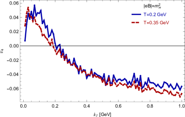
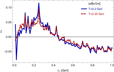
Figure 2: Anisotropic coefficient $v_{4}$ for the photon emission as a function of the transverse momentum $k_{T}$ for two different temperatures, $T=0.2~{}\mbox{GeV}$ (blue) and $T=0.35~{}\mbox{GeV}$ (red), and two different strengths of the magnetic field, $|eB|=m_{\pi}^{2}$ (panel a) and $|eB|=5m_{\pi}^{2}$ (panel b).

The results reveal a clear qualitative pattern in the behavior of $v_{4}$ as a function of the transverse momentum. At relatively small momenta, $k_{T}\lesssim\sqrt{|eB|}$, $v_{4}$ tends to be positive. However, it becomes negative for $k_{T}\gtrsim\sqrt{|eB|}$. Notably, its absolute values are of the order of $0.05$. Such large $v_{4}$ values can be detectable in heavy-ion collisions if the background contributions due to other effects are under control.

The numerical results for $v_{6}$ are shown in Fig. 3. As before, the left and right panels display the results for two different magnetic fields, $|eB|=m_{\pi}^{2}$ and $|eB|=5m_{\pi}^{2}$, respectively. In both cases, the blue solid and the red dashed lines correspond to two fixed temperatures, i.e., $T=0.2~{}\mbox{GeV}$ and $T=0.35~{}\mbox{GeV}$, respectively. In all cases, the dependence of $v_{6}$ on the transverse momentum reveals similar qualitative features. It changes from a negative value at relatively small momenta, $k_{T}\lesssim\sqrt{|eB|}$, to positive values at relatively large momenta $k_{T}\gtrsim\sqrt{|eB|}$. The absolute values of $v_{6}$ are of order $0.02$, which are quite sizable too.

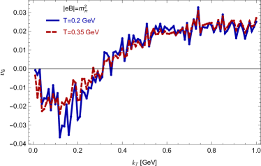
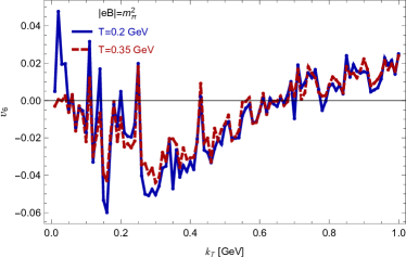
Figure 3: Anisotropic coefficient $v_{6}$ for the photon emission as a function of the transverse momentum $k_{T}$ for two different temperatures, $T=0.2~{}\mbox{GeV}$ (blue) and $T=0.35~{}\mbox{GeV}$ (red), and two different strengths of the magnetic field, $|eB|=m_{\pi}^{2}$ (panel a) and $|eB|=5m_{\pi}^{2}$ (panel b).

The characteristic features of the photon anisotropy are summarized in Table 1. It is interesting to note the alternating signs of the anisotropy coefficients $v_{n}$ with increasing $n$. (Recall that all coefficients with odd $n$ vanish.) Another curious feature is the overall scaling of the magnitude, which goes as $1/n^{2}$. The latter may be an approximate numerical result that holds only for the lowest three nonzero coefficients. However, tentatively it appears to remain true also for $v_{8}$, although the data become less reliable with increasing $n$ when the threshold effects from Landau levels produce many spikes in the angular dependence.

Table 1: Summary of nonvanishing photon and dilepton anisotropy coefficients $v_{n}$.

	$v_{n}$ (photon emission)		$v_{n}$ (dilepton emission)
	$k_{T}\lesssim\sqrt{|eB|}$	$k_{T}\gtrsim\sqrt{|eB|}$	$k_{T}\gtrsim\sqrt{|eB|}$ & $M\lesssim\sqrt{|eB|}$
$v_{2}$	$\simeq-0.2$	$\simeq+0.2$	$\simeq+0.2$
$v_{4}$	$\simeq+0.05$	$\simeq-0.05$	$\simeq-0.05$
$v_{6}$	$\simeq-0.02$	$\simeq+0.02$	$\simeq+0.02$

III.2 Dilepton emission

As demonstrated in Ref. Wang and Shovkovy (2022), dilepton emission from a magnetized hot QGP shows a sizable ellipticity, described by a positive $v_{2}$ of the order of $0.2$, in the kinematic regime of small invariant masses (i.e., $M\lesssim\sqrt{|eB|}$) and large transverse momenta (i.e., $k_{T}\gtrsim\sqrt{|eB|}$). Here we analyze the higher-order anisotropy coefficients $v_{4}$ and $v_{6}$. They also deviate noticeably from zero in the same kinematic regime.

Let us start by first reinforcing the results for the ellipticity of dilepton emission obtained in Ref. Wang and Shovkovy (2022). In particular, here we extend the previous calculations of the ellipticity coefficient $v_{2}$ to larger transverse momenta (up to $k_{T}=2~{}\mbox{GeV}$) and increase the resolution in the invariant mass (i.e., from $\Delta M=0.1~{}\mbox{GeV}$ down to $\Delta M=0.01~{}\mbox{GeV}$). The corresponding new results are shown in Fig. 4. The four panels show the ellipticity coefficient $v_{2}$ as a function of the invariant mass for two temperatures, i.e., $T=0.2~{}\mbox{GeV}$ (two left panels) and $T=0.35~{}\mbox{GeV}$ (two right panels), and two magnetic fields $|eB|=m_{\pi}^{2}$ (two top panels) and $|eB|=5m_{\pi}^{2}$ (two bottom panels). For reference, we also included one of the older low-resolution data sets for $k_{T}=0.5~{}\mbox{GeV}$ from Ref. Wang and Shovkovy (2022).

By comparing the dependence of $v_{2}$ on the invariant mass $M$ with the results in Ref. Wang and Shovkovy (2022), we find that the earlier conclusions are not only valid, but they also become more robust with the increasing of the transverse momentum. Furthermore, the current high-resolution data reconfirms that the ellipticity coefficient $v_{2}$ takes generically large positive values ($v_{2}\sim 0.2$) in the region of small invariant masses (i.e., $M\lesssim\sqrt{|eB|}$). Its magnitude is comparable to the photon $v_{2}$ calculated in Ref. Wang et al. (2020). By comparing the data for the two different temperatures in Fig. 4, we also see that the temperature dependence of the dilepton $v_{2}$ is nearly negligible. For the large transverse momenta considered, of course, it should not be surprising. As we will see below, both $v_{4}$ and $v_{6}$ reveal a similarly weak temperature dependence.

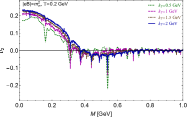
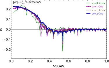
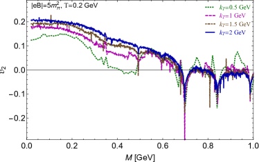
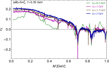
Figure 4: Anisotropic coefficient $v_{2}$ for the dilepton emission as a function of the invariant mass $M$ for several fixed values of the transverse momentum $k_{T}$. The top two panels correspond to $|eB|=m_{\pi}^{2}$, and the bottom two panels to $|eB|=5m_{\pi}^{2}$. The panels on the left are for $T=0.2~{}\mbox{GeV}$, and the ones on the right are for $T=0.35~{}\mbox{GeV}$. The data for $k_{T}=0.5~{}\mbox{GeV}$ is taken from Ref. Wang and Shovkovy (2022).

Now, let us turn to the higher-order anisotropy coefficients $v_{4}$ and $v_{6}$. We will concentrate our attention on the same kinematic region of small invariant masses and large transverse momenta, where the anisotropy is pronounced the most. The numerical results for the dilepton $v_{4}$ as a function of the invariant mass are shown in Fig. 5. As before, the four panels present the results for two temperatures, i.e., $T=0.2~{}\mbox{GeV}$ (two left panels) and $T=0.35~{}\mbox{GeV}$ (two right panels), and two magnetic fields $|eB|=m_{\pi}^{2}$ (two top panels) and $|eB|=5m_{\pi}^{2}$ (two bottom panels). As we see from Fig. 5, at small invariant masses, the coefficient $v_{4}$ tends to be negative with the absolute values of about $0.05$. Note that these are sizable by any reasonable standards. They are also comparable to the $v_{4}$ values in the photon emission at large transverse momenta, see Fig. 2.

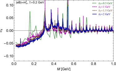
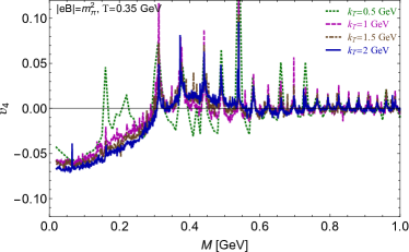
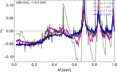
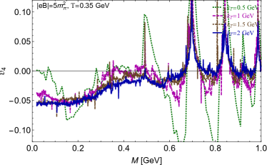
Figure 5: Anisotropic coefficient $v_{4}$ for the dilepton emission as a function of the invariant mass $M$ for several fixed values of the transverse momentum $k_{T}$. The top two panels correspond to $|eB|=m_{\pi}^{2}$, and the bottom two panels to $|eB|=5m_{\pi}^{2}$. The panels on the left are for $T=0.2~{}\mbox{GeV}$, and the ones on the right are for $T=0.35~{}\mbox{GeV}$.

The dilepton results for $v_{6}$ are shown in Fig. 6. The four panels show the results for two temperatures, i.e., $T=0.2~{}\mbox{GeV}$ (two left panels) and $T=0.35~{}\mbox{GeV}$ (two right panels), and two magnetic fields $|eB|=m_{\pi}^{2}$ (two top panels) and $|eB|=5m_{\pi}^{2}$ (two bottom panels). As we see, the anisotropy coefficient $v_{6}$ tends to be positive at small $M$, with the maximal values of the order of $0.02$. Such values are comparable to those of photon $v_{6}$ in Fig. 3.

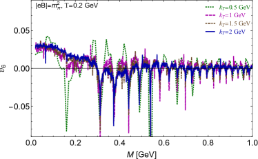
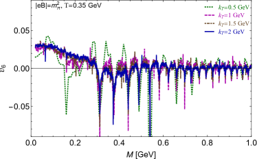
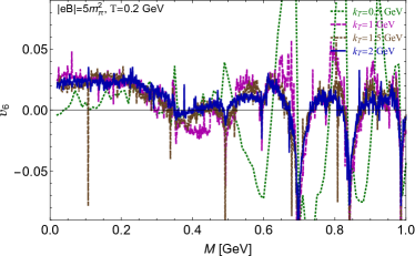
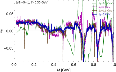
Figure 6: Anisotropic coefficient $v_{6}$ for the dilepton emission as a function of the invariant mass $M$ for several fixed values of the transverse momentum $k_{T}$. The top two panels correspond to $|eB|=m_{\pi}^{2}$, and the bottom two panels to $|eB|=5m_{\pi}^{2}$. The panels on the left are for $T=0.2~{}\mbox{GeV}$, and the ones on the right are for $T=0.35~{}\mbox{GeV}$.

It should be noted, that a nonvanishing $v_{4}$ and $v_{6}$ are barely resolved for the intermediate transverse momentum $k_{T}=0.5~{}\mbox{GeV}$, especially in the case of the stronger field $|eB|=5m_{\pi}^{2}$. It is not surprising as the corresponding $k_{T}$ is comparable to $\sqrt{|eB|}$. Nevertheless, the trend becomes unambiguous for the larger values of $k_{T}$. As anticipated, both $v_{4}$ and $v_{6}$ have a weak temperature dependence at sufficiently large transverse momenta. The key features of the dilepton anisotropy are summarized in Table 1.

In addition to the alternating sign pattern and the hierarchy of coefficients $v_{n}\propto 1/n^{2}$ in the region of small invariant masses, we can also identify other interesting features in the high-resolution data obtained here. For example, we see well-pronounced modulations in the $v_{n}$ dependence on the invariant mass. Indeed, by comparing the results in Figs. 4 through 6, one can easily identify correlated patterns of peaks in all anisotropy coefficients $v_{n}$. They are visible even in the region of moderately large invariant masses. As is easy to verify, they come from the Landau-level quantization of quarks. In heavy-ion physics, such modulations could be hard, if not impossible, to observe. Perhaps, they could have some phenomenological implications in other contexts.

IV Summary and Conclusions

In this paper we investigated the higher-order anisotropy coefficients $v_{4}$ and $v_{6}$ for the photon and dilepton emission from a magnetized hot QGP. For both processes, we revealed several characteristic features in the dependence of the anisotropy coefficients on the kinematic parameters. The summary of the overall magnitudes and signs of the anisotropy coefficients is given in Table 1.

In the case of photon emission, we find qualitatively different anisotropy patterns at small and large transverse momenta. At small momenta (i.e., $k_{T}\lesssim\sqrt{|eB|}$), the signs and absolute values of the anisotropy coefficients are as follows: $v_{4}\simeq+0.05$ and $v_{6}\simeq-0.02$. At large momenta (i.e., $k_{T}\gtrsim\sqrt{|eB|}$), the signs of $v_{n}$ reverse, but the absolute values remain about the same, i.e., $v_{4}\simeq-0.05$ and $v_{6}\simeq+0.02$. Combining these findings with the $v_{2}$ results in Ref. Wang et al. (2020), we see that the signs of even coefficients $v_{n}$ alternate. The absolute values gradually decrease with increasing $n$ in each kinematic region. Quantitatively, the scaling appears to go as $v_{n}\propto 1/n^{2}$

We find that the dilepton emission also has a noticeable anisotropy. However, it is well pronounced only in the kinematic regime with large transverse momenta (i.e., $k_{T}\gtrsim\sqrt{|eB|}$) and small invariant masses (i.e., $M\lesssim\sqrt{|eB|}$). The signs and absolute values of the anisotropy coefficients are as follows: $v_{4}\simeq-0.05$ and $v_{6}\simeq+0.02$. Supplementing these findings with the results for $v_{2}$ obtained in Ref. Wang and Shovkovy (2022), we see that the signs of even coefficients $v_{n}$ alternate, and their absolute values decrease with increasing $n$. The quantitative scaling is similar to that in the photon emission.

In application to QGP produced by noncentral heavy-ion collisions, one may argue that the magnetic field could be too weak, e.g., well below the scale set by the pion mass, to have observable effects. It is possible and, perhaps, even likely that the field is weak indeed. Nevertheless, we argue that even weak fields can affect the anisotropy of both photon and dilepton emissions in certain kinematic regions. Indeed, as we see from our calculations, the anisotropy is sizable even for the transverse momenta that are much larger than the magnetic field scale. This is analogous to the anisotropy of the classical synchrotron radiation. Admittedly, the effects on the photon emission may be diluted by the subleading gluon-mediated processes. Hopefully, the anisotropy does not vanish completely and could remain observable. The situation with dileptons might be better, however. Indeed, the same leading-order diagrams contribute in the case with and without the background magnetic field.

It is tempting to suggest that a set of the first few nonzero anisotropy coefficients $v_{n}$, extracted from the photon and dilepton data, can serve as a distinctive fingerprint of the background magnetic field in a hot QGP produced by heavy-ion collisions. The current data with overwhelming background effects may not allow one to test this idea in experiments. Nevertheless, we find it valuable to have concrete theoretical predictions for $v_{n}$. The advances in experimental techniques and data analysis could make the current hopeless task possible in the future.

Appendix A Imaginary part of the Lorentz-contracted polarization tensor

For convenience, here we quote the expression for the imaginary part of the Lorentz-contracted polarization tensor that appears in the photon and dilepton rates, see Eqs. (2) and (5), respectively. In the Landau-level representation, the corresponding analytical expression takes the following form Wang et al. (2020); Wang and Shovkovy (2021b, 2022):

$$\mbox{Im}\left[\Pi^{\mu}_{R,\mu}\left(\Omega,\mathbf{k}\right)\right] = \sum_{f=u,d}\frac{N_{c}\alpha_{f}}{2\pi l_{f}^{4}}\sum_{n>n^{\prime}}^{\infty}\frac{g(n,n^{\prime})\left\{\Theta\left[(k_{-}^{f})^{2}-k_{\parallel}^{2}\right]-\Theta\left[k_{\parallel}^{2}-(k_{+}^{f})^{2}\right]\right\}}{\sqrt{\left[(k_{-}^{f})^{2}-k_{\parallel}^{2}\right]\left[(k_{+}^{f})^{2}-k_{\parallel}^{2}\right]}}\mathcal{F}_{n,n^{\prime}}^{f}(\xi_{f})$$ (7)

$$- \sum_{f=u,d}\frac{N_{c}\alpha_{f}}{4\pi l_{f}^{4}}\sum_{n=0}^{\infty}\frac{g_{0}(n)\Theta\left[k_{\parallel}^{2}-(k_{+}^{f})^{2}\right]}{\sqrt{k_{\parallel}^{2}\left[k_{\parallel}^{2}-(k_{+}^{f})^{2}\right]}}\mathcal{F}_{n,n^{\prime}}^{f}(\xi_{f}),$$

where $\Theta\left(x\right)$ is the Heaviside step function, $k_{\parallel}^{2}\equiv\Omega^{2}-k_{z}^{2}$, $\xi_{f}=k_{\perp}^{2}\ell_{f}^{2}/2$ and $\ell_{f}=1/\sqrt{|e_{f}B|}$ is a flavor-dependent magnetic length. The Landau-level thresholds are determined by the following two transverse momenta:

$$k_{\pm}^{f}=\left|\sqrt{m^{2}+2n|e_{f}B|}\pm\sqrt{m^{2}+2n^{\prime}|e_{f}B|}\right|.$$ (8)

Functions $g(n,n^{\prime})$ and $g_{0}(n)$ are determined by the quark distributions functions. In thermal equilibrium, they are given by

$$g(n,n^{\prime}) = 2-\sum_{s_{1},s_{2}=\pm}n_{F}\left(\frac{\Omega}{2}+s_{1}\frac{\Omega(n-n^{\prime})|e_{f}B|}{k_{\parallel}^{2}}+s_{2}\frac{|k_{z}|}{2k_{\parallel}^{2}}\sqrt{\left(k_{\parallel}^{2}-(k_{-}^{f})^{2}\right)\left(k_{\parallel}^{2}-(k_{+}^{f})^{2}\right)}\right),$$ (9)

$$g_{0}(n) = g(n,n)=2-2\sum_{s=\pm}n_{F}\left(\frac{\Omega}{2}+s\frac{|k_{z}|}{2|k_{y}|}\sqrt{k_{\parallel}^{2}-4(m^{2}+2n|e_{f}B|)}\right).$$ (10)

Finally, $\mathcal{F}_{n,n^{\prime}}^{f}(\xi)$ is the following flavor-dependent function of the transverse momentum:

$$\mathcal{F}^{f}_{n,n^{\prime}}(\xi)=8\pi\left(n+n^{\prime}+m^{2}\ell_{f}^{2}\right)\left[\mathcal{I}_{0}^{n,n^{\prime}}(\xi)+\mathcal{I}_{0}^{n-1,n^{\prime}-1}(\xi)\right]+8\pi\left(\frac{k_{\parallel}^{2}-k_{\perp}^{2}}{2}\ell_{f}^{2}-(n+n^{\prime})\right)\left[\mathcal{I}_{0}^{n,n^{\prime}-1}(\xi)+\mathcal{I}_{0}^{n-1,n^{\prime}}(\xi)\right],$$ (11)

and function $\mathcal{I}_{0}^{n,n^{\prime}}(\xi)$ is defined in terms of the Laguerre polynomials, i.e.,

$$\mathcal{I}_{0}^{n,n^{\prime}}(\xi)=\frac{(n^{\prime})!}{n!}e^{-\xi}\xi^{n-n^{\prime}}\left(L_{n^{\prime}}^{n-n^{\prime}}\left(\xi\right)\right)^{2}=\frac{n!}{(n^{\prime})!}e^{-\xi}\xi^{n^{\prime}-n}\left(L_{n}^{n^{\prime}-n}\left(\xi\right)\right)^{2}.$$ (12)

Note that the two different representations for $\mathcal{I}_{0}^{n,n^{\prime}}(\xi)$ are equivalent.

References

- Yagi et al. (2005) K. Yagi, T. Hatsuda, and Y. Miake, Quark-Gluon Plasma: From Big Bang to Little Bang, Vol. 23 (Cambridge University Press, Cambridge, UK, 2005).
- Rischke (2004) D. H. Rischke, Prog. Part. Nucl. Phys. 52, 197 (2004), arXiv:nucl-th/0305030 .
- Shuryak (2017) E. Shuryak, Rev. Mod. Phys. 89, 035001 (2017), arXiv:1412.8393 [hep-ph] .
- Gross and Wilczek (1973) D. J. Gross and F. Wilczek, Phys. Rev. Lett. 30, 1343 (1973).
- Politzer (1973) H. D. Politzer, Phys. Rev. Lett. 30, 1346 (1973).
- Bzdak et al. (2020) A. Bzdak, S. Esumi, V. Koch, J. Liao, M. Stephanov, and N. Xu, Phys. Rept. 853, 1 (2020), arXiv:1906.00936 [nucl-th] .
- Back et al. (2005) B. B. Back et al. (PHOBOS), Nucl. Phys. A 757, 28 (2005), arXiv:nucl-ex/0410022 .
- Adcox et al. (2005) K. Adcox et al. (PHENIX), Nucl. Phys. A 757, 184 (2005), arXiv:nucl-ex/0410003 .
- Adams et al. (2005) J. Adams et al. (STAR), Nucl. Phys. A 757, 102 (2005), arXiv:nucl-ex/0501009 .
- Heinz and Snellings (2013) U. Heinz and R. Snellings, Ann. Rev. Nucl. Part. Sci. 63, 123 (2013), arXiv:1301.2826 [nucl-th] .
- Bernhard et al. (2019) J. E. Bernhard, J. S. Moreland, and S. A. Bass, Nature Phys. 15, 1113 (2019).
- Skokov et al. (2009) V. Skokov, A. Y. Illarionov, and V. Toneev, Int. J. Mod. Phys. A24, 5925 (2009), arXiv:0907.1396 .
- Voronyuk et al. (2011) V. Voronyuk, V. Toneev, W. Cassing, E. Bratkovskaya, V. Konchakovski, et al., Phys. Rev. C83, 054911 (2011), arXiv:1103.4239 .
- Deng and Huang (2012) W.-T. Deng and X.-G. Huang, Phys. Rev. C85, 044907 (2012), arXiv:1201.5108 .
- Bloczynski et al. (2013) J. Bloczynski, X.-G. Huang, X. Zhang, and J. Liao, Phys. Lett. B718, 1529 (2013), arXiv:1209.6594 .
- Tuchin (2016) K. Tuchin, Phys. Rev. C 93, 014905 (2016), arXiv:1508.06925 [hep-ph] .
- Guo et al. (2020) X. Guo, J. Liao, and E. Wang, Sci. Rep. 10, 2196 (2020), arXiv:1904.04704 [hep-ph] .
- Fukushima et al. (2008) K. Fukushima, D. E. Kharzeev, and H. J. Warringa, Phys. Rev. D78, 074033 (2008), arXiv:0808.3382 .
- Kharzeev and Zhitnitsky (2007) D. Kharzeev and A. Zhitnitsky, Nucl. Phys. A797, 67 (2007), arXiv:0706.1026 .
- Kharzeev et al. (2008) D. E. Kharzeev, L. D. McLerran, and H. J. Warringa, Nucl. Phys. A803, 227 (2008), arXiv:0711.0950 .
- Tuchin (2013a) K. Tuchin, Adv. High Energy Phys. 2013, 490495 (2013a), arXiv:1301.0099 [hep-ph] .
- Kharzeev et al. (2016) D. E. Kharzeev, J. Liao, S. A. Voloshin, and G. Wang, Prog. Part. Nucl. Phys. 88, 1 (2016), arXiv:1511.04050 .
- Huang (2016) X.-G. Huang, Rept. Prog. Phys. 79, 076302 (2016), arXiv:1509.04073 .
- Miransky and Shovkovy (2015) V. A. Miransky and I. A. Shovkovy, Phys. Rept. 576, 1 (2015), arXiv:1503.00732 .
- Yee (2013) H.-U. Yee, Phys. Rev. D 88, 026001 (2013), arXiv:1303.3571 [nucl-th] .
- Tuchin (2015) K. Tuchin, Phys. Rev. C 91, 014902 (2015), arXiv:1406.5097 [nucl-th] .
- Zakharov (2016) B. G. Zakharov, Eur. Phys. J. C 76, 609 (2016), arXiv:1609.04324 [nucl-th] .
- Tuchin (2013b) K. Tuchin, Phys. Rev. C88, 024910 (2013b), arXiv:1305.0545 .
- Adare et al. (2012) A. Adare et al. (PHENIX), Phys. Rev. Lett. 109, 122302 (2012), arXiv:1105.4126 .
- Adare et al. (2016) A. Adare et al. (PHENIX), Phys. Rev. C94, 064901 (2016), arXiv:1509.07758 .
- Acharya et al. (2019) S. Acharya et al. (ALICE), Phys. Lett. B789, 308 (2019), arXiv:1805.04403 .
- Chatterjee et al. (2006) R. Chatterjee, E. S. Frodermann, U. W. Heinz, and D. K. Srivastava, Phys. Rev. Lett. 96, 202302 (2006), arXiv:nucl-th/0511079 .
- Schenke and Strickland (2007) B. Schenke and M. Strickland, Phys. Rev. D76, 025023 (2007), arXiv:hep-ph/0611332 .
- Chatterjee and Srivastava (2009) R. Chatterjee and D. K. Srivastava, Phys. Rev. C 79, 021901 (2009), arXiv:0809.0548 [nucl-th] .
- van Hees et al. (2011) H. van Hees, C. Gale, and R. Rapp, Phys. Rev. C 84, 054906 (2011), arXiv:1108.2131 [hep-ph] .
- Linnyk et al. (2014) O. Linnyk, W. Cassing, and E. L. Bratkovskaya, Phys. Rev. C 89, 034908 (2014), arXiv:1311.0279 [nucl-th] .
- Gale et al. (2015) C. Gale, Y. Hidaka, S. Jeon, S. Lin, J.-F. Paquet, R. D. Pisarski, D. Satow, V. V. Skokov, and G. Vujanovic, Phys. Rev. Lett. 114, 072301 (2015), arXiv:1409.4778 [hep-ph] .
- Muller et al. (2014) B. Muller, S.-Y. Wu, and D.-L. Yang, Phys. Rev. D89, 026013 (2014), arXiv:1308.6568 .
- van Hees et al. (2015) H. van Hees, M. He, and R. Rapp, Nucl. Phys. A 933, 256 (2015), arXiv:1404.2846 [nucl-th] .
- Monnai (2014) A. Monnai, Phys. Rev. C 90, 021901 (2014), arXiv:1403.4225 [nucl-th] .
- Dion et al. (2011) M. Dion, J.-F. Paquet, B. Schenke, C. Young, S. Jeon, and C. Gale, Phys. Rev. C 84, 064901 (2011), arXiv:1109.4405 [hep-ph] .
- Liu and Liu (2014) F.-M. Liu and S.-X. Liu, Phys. Rev. C 89, 034906 (2014), arXiv:1212.6587 [nucl-th] .
- Vujanovic et al. (2014) G. Vujanovic, J.-F. Paquet, G. S. Denicol, M. Luzum, B. Schenke, S. Jeon, and C. Gale, Nucl. Phys. A 932, 230 (2014), arXiv:1404.3714 [hep-ph] .
- McLerran and Schenke (2014) L. McLerran and B. Schenke, Nucl. Phys. A 929, 71 (2014), arXiv:1403.7462 [hep-ph] .
- McLerran and Schenke (2016) L. McLerran and B. Schenke, Nucl. Phys. A 946, 158 (2016), arXiv:1504.07223 [nucl-th] .
- Gelis et al. (2004) F. Gelis, H. Niemi, P. V. Ruuskanen, and S. S. Rasanen, J. Phys. G 30, S1031 (2004), arXiv:nucl-th/0403040 .
- Hidaka et al. (2015) Y. Hidaka, S. Lin, R. D. Pisarski, and D. Satow, JHEP 10, 005 (2015), arXiv:1504.01770 [hep-ph] .
- Linnyk et al. (2016) O. Linnyk, E. L. Bratkovskaya, and W. Cassing, Prog. Part. Nucl. Phys. 87, 50 (2016), arXiv:1512.08126 [nucl-th] .
- Vovchenko et al. (2016) V. Vovchenko, I. A. Karpenko, M. I. Gorenstein, L. M. Satarov, I. N. Mishustin, B. Kämpfer, and H. Stoecker, Phys. Rev. C 94, 024906 (2016), arXiv:1604.06346 [nucl-th] .
- Koide and Kodama (2016) T. Koide and T. Kodama, J. Phys. G 43, 095103 (2016), arXiv:1605.05127 [nucl-th] .
- Turbide et al. (2006) S. Turbide, C. Gale, and R. J. Fries, Phys. Rev. Lett. 96, 032303 (2006), arXiv:hep-ph/0508201 .
- Tuchin (2013c) K. Tuchin, Phys. Rev. C 87, 024912 (2013c), arXiv:1206.0485 [hep-ph] .
- Basar et al. (2012) G. Basar, D. Kharzeev, and V. Skokov, Phys. Rev. Lett. 109, 202303 (2012), arXiv:1206.1334 .
- Wang et al. (2020) X. Wang, I. A. Shovkovy, L. Yu, and M. Huang, Phys. Rev. D 102, 076010 (2020), arXiv:2006.16254 .
- Wang and Shovkovy (2021a) X. Wang and I. Shovkovy, Eur. Phys. J. C 81, 901 (2021a), arXiv:2106.09029 [nucl-th] .
- Rapp and van Hees (2016) R. Rapp and H. van Hees, Phys. Lett. B 753, 586 (2016), arXiv:1411.4612 [hep-ph] .
- Sadooghi and Taghinavaz (2017) N. Sadooghi and F. Taghinavaz, Annals Phys. 376, 218 (2017), arXiv:1601.04887 .
- Bandyopadhyay et al. (2016) A. Bandyopadhyay, C. A. Islam, and M. G. Mustafa, Phys. Rev. D 94, 114034 (2016), arXiv:1602.06769 [hep-ph] .
- Bandyopadhyay and Mallik (2017) A. Bandyopadhyay and S. Mallik, Phys. Rev. D95, 074019 (2017), arXiv:1704.01364 .
- Ghosh and Chandra (2018) S. Ghosh and V. Chandra, Phys. Rev. D98, 076006 (2018), arXiv:1808.05176 .
- Islam et al. (2019) C. A. Islam, A. Bandyopadhyay, P. K. Roy, and S. Sarkar, Phys. Rev. D99, 094028 (2019), arXiv:1812.10380 .
- Das et al. (2019) A. Das, N. Haque, M. G. Mustafa, and P. K. Roy, Phys. Rev. D99, 094022 (2019), arXiv:1903.03528 .
- Ghosh et al. (2020) S. Ghosh, N. Chaudhuri, S. Sarkar, and P. Roy, Phys. Rev. D 101, 096002 (2020), arXiv:2004.09203 [nucl-th] .
- Chaudhuri et al. (2021) N. Chaudhuri, S. Ghosh, S. Sarkar, and P. Roy, Phys. Rev. D 103, 096021 (2021), arXiv:2104.11425 [hep-ph] .
- Das et al. (2022) A. Das, A. Bandyopadhyay, and C. A. Islam, Phys. Rev. D 106, 056021 (2022), arXiv:2109.00019 [hep-ph] .
- Wang and Shovkovy (2022) X. Wang and I. A. Shovkovy, Phys. Rev. D 106, 036014 (2022), arXiv:2205.00276 [nucl-th] .
- Kapusta and Gale (2011) J. I. Kapusta and C. Gale, Finite-Temperature Field Theory: Principles and Applications, Cambridge Monographs on Mathematical Physics (Cambridge University Press, 2011).
- Wang and Shovkovy (2021b) X. Wang and I. Shovkovy, Phys. Rev. D 104, 056017 (2021b), arXiv:2103.01967 [nucl-th] .
- Kapusta et al. (1991) J. I. Kapusta, P. Lichard, and D. Seibert, Phys. Rev. D 44, 2774 (1991), [Erratum: Phys.Rev.D 47, 4171 (1993)].
- Baier et al. (1992) R. Baier, H. Nakkagawa, A. Niegawa, and K. Redlich, Z. Phys. C 53, 433 (1992).
- Aurenche et al. (1998) P. Aurenche, F. Gelis, R. Kobes, and H. Zaraket, Phys. Rev. D 58, 085003 (1998), arXiv:hep-ph/9804224 .
- Steffen and Thoma (2001) F. D. Steffen and M. H. Thoma, Phys. Lett. B 510, 98 (2001), [Erratum: Phys.Lett.B 660, 604–606 (2008)], arXiv:hep-ph/0103044 .
- Arnold et al. (2001a) P. B. Arnold, G. D. Moore, and L. G. Yaffe, JHEP 11, 057 (2001a), arXiv:hep-ph/0109064 .
- Arnold et al. (2001b) P. B. Arnold, G. D. Moore, and L. G. Yaffe, JHEP 12, 009 (2001b), arXiv:hep-ph/0111107 .
- Ghiglieri et al. (2013) J. Ghiglieri, J. Hong, A. Kurkela, E. Lu, G. D. Moore, and D. Teaney, JHEP 05, 010 (2013), arXiv:1302.5970 [hep-ph] .
- Cleymans et al. (1987) J. Cleymans, J. Fingberg, and K. Redlich, Phys. Rev. D 35, 2153 (1987).