Uncovering Local Integrability in Quantum Many-Body Dynamics

Interacting many-body quantum systems and their dynamics, while fundamental to modern science and technology, are formidable to simulate and understand. However, by discovering their symmetries, conservation laws, and integrability one can unravel their intricacies. Here, using up to 124 qubits of a fully programmable quantum computer, we uncover local conservation laws and integrability in one- and two-dimensional periodically-driven spin lattices in a regime previously inaccessible to such detailed analysis. We focus on the paradigmatic example of disorder-induced ergodicity breaking, where we first benchmark the system crossover into a localized regime through anomalies in the one-particle-density-matrix spectrum and other hallmark signatures. We then demonstrate that this regime stems from hidden local integrals of motion by faithfully reconstructing their quantum operators, thus providing a detailed portrait of the system’s integrable dynamics. Our results demonstrate a versatile strategy for extracting hidden dynamical structure from noisy experiments on large-scale quantum computers.

A quantum system is entirely characterized by knowledge of its energy levels and wavefunctions—in principle. In practice, however, systems comprising numerous interacting particles lie beyond the jurisdiction of such a description. Their exponentially numerous levels, vanishing inter-level spacings, and substantial computational and resource costs render this approach impractical. Nonetheless, these complex systems often harbor latent structure that, if discovered, could unlock a tractable description. In classical physics, for example, the identification of a comprehensive set of conserved quantities, or integrals of motion that are often associated with symmetries, yields such an analogous description [arnol2013mathematical].

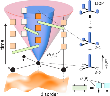
Fig. 1: Many-body dynamics: quantum simulation and integrals of motion. Four interacting spins (black circles) undergoing time-periodic dynamics in a modified kicked Ising model with random on-site disorder—modeled as a digital quantum circuit. Disorder is represented by single-qubit phase gates $P(\phi_{i})$ with site-randomized angles $\phi_{i}$ (colored squares). Uniform spin-spin interactions (green rectangles) are mediated by controlled-Z gates followed by rotations $U$ of strength $\theta$, defined in Eq. (1). In the ergodic regime, quantum operators spread rapidly (wide cone). Sufficient disorder can remarkably slow down spreading the operators, leading to the many-body localization regime (blue cone). Disruptions to ergodicity due to integrability result in hidden conserved quantities linked to local integral of motion (LIOM) operators. We experimentally extract a complete set of LIOMs from the system’s time evolution by averaging operators spread.

Quantum physics presents a fundamentally more intricate scenario. Integrals of motion can exist—they are now operators that remain unchanged under system evolution and can be used to define good quantum numbers. When the number of these operators scales extensively with the system size, the system can be regarded as quantum integrable [caux2011remarks], which can help to unravel its complexity [sutherland2004beautiful]. For instance, the occupation operators corresponding to single-fermion eigenstates in a free-fermion model form a complete set of integrals of motion. Their eigenvalues can be employed to find and label all eigenstates. This non-interacting system is integrable. Unfortunately, for interacting particles, even proving the existence of non-trivial integrals of motion is an intractable mathematical problem [shiraishi2021undecidability], let alone to quantitatively find them. Can large-scale quantum experiments help us with this problem?

Our work aims to identify local conserved operators—commonly referred to as local integrals of motion (LIOMs)—through experiments on a quantum computer. We focus on a broad class of disordered systems that exhibit many-body localization (MBL) [basko2006metal, pal2010mbl, nandkishore2015many, abanin2019colloq]. In these systems, strong disorder is thought to suppress the transfer of energy and information across the system, leading to an effective description by a complete set of LIOMs [serbyn2013lioms, huse2014lioms]. While the ultimate stability of the MBL for thermodynamically-large systems remains a topic of debate [wdroeck2017stability, morningstar2022avalanches, sels2022avalanches, leonard2023probing], its main properties—including slow entanglement growth and absence of equilibration—can be reliably observed for limited system sizes, as has recently been found in numerous experiments [rispoli2019quantum, lukin2019probing, roushan2017spectroscopic, choi2016exploring, schreiber2015experiment, smith2016experiment, bordia2017experiment, bordia2017experiment_2d, guo2021experiment, mi2022time]. This scenario is referred to as the finite-size MBL regime [morningstar2022avalanches].

Strictly speaking, for universal dynamics, operators extracted from any finite-time analysis are approximate and, thus, not exactly conserved. Thus, one should be cautious in using them as evidence for the ultimate integrability of the system. One can imagine a scenario where approximate LIOMs exist, but the construction of exact LIOMs becomes impossible [sels2023thermalization]. Such systems may behave as nearly-integrable for some time, but eventually become chaotic. In the absence of evidence of integrability in the system, we call these approximate operators prethermal LIOMs. They can thus provide an efficient description of the system on the timescales of observation.

To construct sets of approximate LIOMs, we devise general protocols, including those for detecting prerequisite conditions such as ergodicity violations—a primary signature of integrability. We perform all experiments on 1D and 2D spin systems, using circuits of up to 124 qubits and depth 60. Crucially, we exploit the quantum processor’s large size for overcoming finite-size effects in 2D, its programmability for measurements in non-commuting bases, and its operational speed to execute vast numbers of unique digital circuits (over 350,000). We address device noise through the resilience of our protocol and a tailored error-mitigation workflow [supplement].

Our spin system, akin to the paradigmatic kicked Ising model, undergoes periodic time evolution (see Fig. 1), or Floquet dynamics. Each evolution cycle is a unitary $U_{F}$, implemented as a series of gates on two IBM quantum processors, ibmq_kolkata and ibm_washington. The cycle is built from two-qubit gates (green rectangles in Fig. 1) comprising controlled-Z gates followed by the parameterized single-qubit gates (blue squares)

$$U(\theta)\coloneqq\begin{pmatrix}\cos\theta/2&\sin\theta/2\\ \sin\theta/2&-\cos\theta/2\\ \end{pmatrix}\;\;\mathrm{and}\;\;P(\phi_{k})\coloneqq\begin{pmatrix}1&0\\ 0&e^{i\phi_{k}}\\ \end{pmatrix}\;.$$ (1)

The unitary $U$ introduces transverse field kicks, for non-zero angles $\theta\in[0,\pi/2]$ and $P$ introduces disorder through random phases $\phi_{k}\in[-\pi,\pi]$ uniformly sampled over each spin site $k$.

For $\theta=0$, the system dynamics are non-universal and integrable. In 1D, we expect integrability to be present at small angles $\theta<\theta_{c}$ for some non-zero critical $\theta_{c}$ according to the MBL hypothesis. Disorder inhibits spread of correlations (narrow cone in Fig. 1), and leads to an MBL regime [zhang2016floquet, ponte2015floquetmbl, bordia2017experiment]. In contrast, for $\theta_{c}<\theta\leq\pi/2$, the system’s integrability is replaced by chaotic behavior leading to local operators irreversibly spreading into non-local and high-weight ones (wide cone) [nahum2018operator].

To confirm these predictions, we first subject our model to the necessary benchmarks. Starting with the more tractable 1D case, using small-system classical numerics, we validate the existence of a critical angle $\theta_{c}\approx 0.16\pi$ that separates the ergodic and MBL regimes [supplement]. Below, we present the corresponding experiments, before studying LIOMs in 1D and 2D.

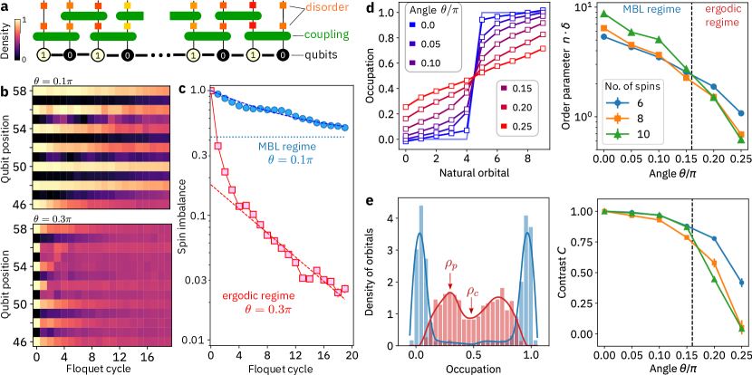
Fig. 2: Conventional benchmark experiments of localization in the 1D model. a. A 104-qubit chain initialized with an antiferromagnetic pattern evolves under a circuit comprising $\theta$-parametrized two-qubit gates (rectangles) and single-qubit disorder gates (squares). Depicted is a single Floquet cycle, which is repeated multiple times. The color of the gates indicates different disorder angles $\phi_{i}$. b. Spin density evolution in two distinct regimes: many-body localized (MBL) at $\theta=0.1\,\pi$ and ergodic at $\theta=0.3\,\pi$. c. The spin imbalance $\mathcal{I}$ is indicative of the preservation of initial state memory. In the ergodic regime, the imbalance (red squares) decays within a few Floquet cycles, the exponential late decay to zero imbalance is shown as a red dashed line. In the MBL regime, the imbalance (blue circles) persists, the dotted line shows the saturation point at $\mathcal{I}\approx 0.42$, derived from an exponential curve fit (blue dashed line). d. One-particle density matrix (OPDM) spectra after 9 Floquet cycles. Left: OPDM spectra for a 10-qubit chain averaged over 100 disorders; initial-state spectrum in faded blue. Residual spectrum discontinuity is conspicuous for small $\theta$. Right: Rescaled discontinuity across different system sizes, intersecting near the suggested critical point $\theta_{c}\approx 0.16\,\pi$. e. Peak-to-gap density contrast in OPDM spectrum. Left: State densities for 10 qubits in the MBL ($\theta=0.05\,\pi$, blue) and ergodic ($\theta=0.2\,\pi$, red) regimes. Right: Contrast as a function of $\theta$. As expected, it saturates in the MBL regime and decreases with system size in the ergodic regime. In all panels, statistical error is typically smaller than marker size.

First signature of ergodicity breaking: Memory. We initialize a 104-qubit, 1D spin chain in a space-periodic antiferromagnetic pattern [schreiber2015experiment, smith2016experiment] depicted in Fig. 2a. We evolve the system under a fixed disorder realization for $\theta=0.1\pi$ and $\theta=0.3\pi$ and record error-mitigated snapshots of its spins’ polarizations (see Fig. 2b). Memory of the initial antiferromagnetic state is quantified through the spin imbalance $\mathcal{I}\coloneqq\frac{n_{1}-n_{0}}{n_{1}+n_{0}}$ defined as the normalized difference between the average polarization of the sites initialized in state zero (spin up) and one (spin down), $n_{0}$ and $n_{1}\in[0,1]$, respectively.

At $\theta=0.3\pi$ (see Fig. 2c), the order parameter $\mathcal{I}$ decays precipitously within 20 Floquet cycles. This suggests that the transverse field overpowers disorder and points to an ergodic regime and quantum information scrambling. Conversely, at $\theta=0.1\pi$, the preservation of $\mathcal{I}$, or the retention of the antiferromagnetic pattern, suggests that disorder prevails and results in preservation of local memory of the initial state, as expected in the MBL regime.

Second signature: Anomalies in the one-particle density matrix (OPDM). To obtain a more direct indicator of the MBL and ergodic regimes, we consider the spin system as a lattice of interacting hardcore bosons (site can have at most one excitation), with $|0\rangle$ and $|1\rangle$ representing unoccupied and occupied sites, respectively. The indicator is provided through the OPDM [bera2015opdm, bera2017opdm], which we generalize as

$$\rho_{ij}=\langle a^{\dagger}_{i}a_{j}\rangle-\langle a^{\dagger}_{i}\rangle\langle a_{j}\rangle\;,$$ (2)

where $a_{i}=\frac{1}{2}(X_{i}-iY_{i})$ is the Fock annihilation operator for a hardcore boson at site $i$ and $\langle\,\cdot\,\rangle$ represents expectation with respect to the system state. The last term is used to account for the uncorrelated dynamics in a particle-non-conserving system.

Experimentally, we first prepare the system in an antiferromagnetic many-body state, whose OPDM spectrum contains only eigenvalues one and zero, interpretable as the system comprising natural orbitals that are either ‘occupied’ or ‘empty’. We time-evolve the system and construct the OPDM from a logarithmic set of bit strings measured in $X$ or $Y$ basis randomly chosen for each qubit [elben2023randomized]. Owing to the limited connectivity in 1D, it is sufficient to restrict our attention to smaller qubit subchains to capture the significant correlations.

In the left panel of Fig. 2d, we report the OPDM spectrum of 10 spins after 9 Floquet cycles, averaged over 100 disorder realizations and as a function of $\theta$. For small $\theta$, half the OPDM eigenstates, or natural orbitals, are nearly occupied and the other half are nearly empty—disorder has frozen the system’s evolution. A conspicuous discontinuity (gap) $\delta$ in the center of the spectrum persists despite the evolution under interactions—a robust signature of stable quasiparticles [mahan2000many]. On the other hand, for large $\theta$, the discontinuity vanishes and the spectra look ergodic.

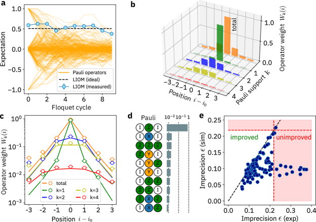
Fig. 3: Uncovering local integrals of motion (LIOM) operators in 1D. a. Example measurements for a typical LIOM; for the initial state $|000011\rangle^{\otimes 17}|00\rangle$ and initial guess $L^{(0)}=Z_{50}$. The time-dependent expectation values of the numerous local Pauli operators composing the LIOM are displayed in orange, while the reconstructed expectations of the LIOMs are indicated by blue dots. A comparable ideal, noise-free LIOM, derived from exact diagonalization for a subsystem encompassing qubits 44 to 56, is represented by the dashed line. b. Experimental reconstruction of the average of LIOM operators in the bulk of a 104-qubit chain, extracted over 9 Floquet cycles, depicted over both space and Pauli support. Orange bars depict the total LIOM weights. Remaining bars show the individual contributions of Pauli operators with support one (green), two (blue), three (yellow), and four (red). c. Same data (dots) compared against ideal, noiseless numerical simulation (log plot). The error bars represent bootstrapped error estimates. d. Average LIOM structure in terms of dominant Pauli operators depicted by average operator weights $w_{\mu}$ (log scale) on the right. e. Imprecision $\epsilon$ (defined in the text) of the 104 LIOMs in noiseless simulation (y-axis) and in experiment (x-axis) for $\theta=0.1\,\pi$. Red regions indicate error values exceeding the imprecision $\epsilon_{0}$ of the initial guesses $L^{(0)}_{i}=Z_{i}$ for $i\in[1,103]$.

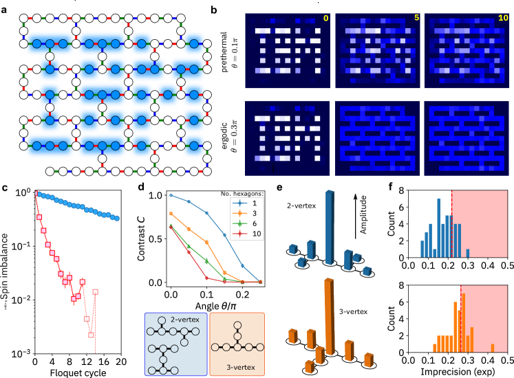
Fig. 4: Benchmark signatures and uncovering LIOM operators in 2D. a. The 124-qubits (circles) of the heavy-hexagonal ibm_washington processor used in the 2D experiments. Edge colors (blue, green, red) signify time order of two-qubit gates in a Floquet cycle. Arbitrary initial-excitation patterns can be encoded: blue fill for $|1\rangle$ and white for $|0\rangle$ initialization. b. Color-coded visualization of single-qubit excitations (white represents 1, dark blue 0) across the entire device for Floquet cycles $m=0$, 5, and 10, at two interactions: $\theta=0.1\pi$ (top) and $\theta=0.3\pi$ (bottom). Pattern diffusion at $\theta=0.1\pi$ suggests prethermalization. c. Spin imbalance for an initial antiferromagnetic pattern. Error bars shown as vertical sticks behind markers. For $\theta=0.3\pi$ (red), signal is vanishing beyond cycle 10. For $\theta=0.1\pi$ (blue), gradual relaxation is observed without an evident plateau. d. OPDM gap contrast versus interaction strength $\theta$ across system sizes measured in number of hexagon rings [supplement]. Clear signature of MBL regime is not evident. Statistical error is smaller than the marker size. e. In 2D, LIOMs have two unique support topologies characterized by a central vertex with either two or three connections. Average LIOM operator weights in the bulk for each topology are shown (representing a total of 124 LIOMs). f. Imprecision histograms for all bulk two-vertex (top) and three-vertex (bottom) prethermal LIOMs. The shaded region indicates imprecision that exceeds that of the initial-guess operator.

To understand scaling with system size $n$, in the right panel of Fig. 2d, we plot the order parameter $\delta\times n$. With increasing system size, this quantity should theoretically diverge in the MBL regime but vanish in the ergodic regime, where thermalization leads to a featureless ‘infinite-temperature’ state, and a cross-over between the two should be present. Experimentally, we observe the anticipated crossover at $\theta\approx 0.16\pi$, in agreement with the critical angle $\theta_{c}$ obtained from the exact diagonalization.

The spectral discontinuity $\delta$ is sensitive to experimental noise, which could also close it. As a more noise-robust order parameter, we introduce the gap contrast $C\coloneqq 1-\rho_{c}/\rho_{p}$, where $\rho_{c}$ is the density of orbitals (i.e. average number of orbitals per range of occupation values) at the center of the spectrum and $\rho_{p}$ is the value at the density peaks; see Fig. 2e. We introduce this quantity here to observe the spectral signatures of the MBL even when the noise effects transform the spectral gap into a ‘soft gap’, where the density of states is low but non-vanishing. The contrast $C$ is maximized for noiseless MBL dynamics ($C=1$) and vanishes for ergodic dynamics ($C=0$). Our experimental observations in Fig. 2e align with the expected behavior.

Local integrals of motion (LIOMs) in 1D. To find a comprehensive description of the MBL regime and its integrability, we develop an experimental protocol, inspired by Refs. [mierzejewski2015identifying, chandran2015constructing], to construct a system’s LIOMs $L_{1},L_{2}\dots,L_{n}$ from its time dynamics (recall Fig. 1). Here, a LIOM $L$ is a Hermitian operator that commutes with the Floquet unitary $[L,U_{F}]=0$ and corresponds to a conserved quantity. It admits a decomposition $L=\sum_{\mu}a_{\mu}P_{\mu}$ over multi-qubit Pauli operators $P_{\mu}$ indexed by $\mu\in[1,4^{n}]$, with real-valued weights $a_{\mu}$ that we aim to determine. To do so, we use the fact that average inverse-time evolution of an arbitrary initial operator $L^{(0)}$ is an exact LIOM [mierzejewski2015identifying, chandran2015constructing]. The Pauli weights for this operator are

$$a_{\mu}=\frac{1}{2^{n}}\lim_{D\to\infty}\frac{1}{D+1}\sum_{d=0}^{D}{\rm Tr\,}\left[U^{d}_{F}L^{(0)}U^{d{\dagger}}_{F}P_{\mu}\right]\;,$$ (3)

where $D$ is the number of Floquet cycles. The choice of the initial guess strongly affects the convergence of the sum [supplement].

To experimentally estimate $a_{\mu}$, we first measure [elben2023randomized] the time evolution of Pauli expectation values $\langle P_{\mu}(d)\rangle$; see Fig. 3a. To minimize the impact of noise, we limit $D$ to 10 cycles. For each qubit $i$, we select $L^{(0)}_{i}=Z_{i}$, the on-site $Z$ operator. As depicted for $i=50$ in Fig. 3a, we find a combination of the numerous expectation values that yields an approximate constant of motion (blue dots) or LIOM. As the data show, the apparent chaos of expectation values hides order.

To understand the effect of noise and partially validate the LIOM, we find the exact LIOM in the absence of noise for a 10-qubit subset of the 1D chain. The dashed line reports the noise-free LIOM value, aligning with the data up to some small variance, which we will shortly use to quantify the precision of the extracted LIOMs.

We next extract 104 different LIOMs for the 1D chain. One should expect that LIOMs must be linear combinations of Pauli operators with weights that decay exponentially with the distance from the center and the size of the Pauli operators. To illuminate this structure, we evaluate $k$-local qubit weights $W_{k}(i)\coloneqq\sqrt{\sum_{\mu}a_{\mu}^{2}\delta(i,k,\mu)}$, where $\delta(i,k,\mu)$ is equal to $1/k$ if $P_{\mu}$ acts non-trivially on $k$ qubits necessarily including qubit $i$; otherwise, $\delta(i,k,\mu)=0$. Fig. 3b shows the average weights $W_{k}(i-i_{0})$ for bulk LIOMs generated from Pauli-Z operators on qubits $i_{0}\in[6,97]$, along with the total weights $W(i)=\sqrt{\sum_{k}W^{2}_{k}(i)}$. The data clearly show the striking exponential localization of the LIOMs in both distance $|i-i_{0}|$ from their centers $i_{0}$ and higher-weight operator locality $k$.

How good is the average reconstruction? In Fig. 3c, we compare the experimental data (dots) with noise-free simulations (solid lines) obtained from brute-force simulations of a subsystem within the physical lightcone. The two agree notably across several orders of magnitude.

To gain further insight, we also evaluate an average LIOM characterized by normalized weights $w_{\mu}=\operatorname{\mathbb{E}}[a^{2}_{\mu}]$ averaged over the bulk LIOMs when we align their centers. We depict dominant Pauli contributions in Fig. 3d, which evidently originate primarily from a few local Pauli operators. The central Pauli-Z dominates with $w_{Z}=0.71$—an observation in alignment with the robustness of the spin imbalance of the antiferromagnetic order observed in the benchmark experiments in Fig. 2a. Additionally, the central Paulis $X$ and $Y$ are also partially conserved, albeit with significantly lower average residual expectations of $w_{X}=0.021$ and $w_{Y}=0.016$.

Precision of the individual LIOMs in 1D. By their finite-time construction, the LIOMs are strictly-speaking only approximate. We quantify the quality of the LIOMs by the normalized error in their commutator with the Floquet cycle unitary, $\epsilon=\|[L,U_{F}]\|_{F}/2\|L\|_{F}$, where $\|\cdot\|_{F}$ is the Frobenius norm. Notably, numerical evaluation of this LIOM imprecision $\epsilon$ is only polynomial in the number of Pauli terms and their locality. Moreover, it is independent of the number of qubits for large systems. For our initial guess $L^{(0)}=Z_{i}$, the imprecision is $\epsilon_{0}=\sin\theta/\sqrt{2}$ ($\approx 0.2185$ for $\theta=0.1\pi$) regardless of the qubit index $i$ and disorder realization. If successful, our protocol should find operators with lower $\epsilon$. If the system slowly thermalizes for times $D\gg 10$, in which case we refer to the operators as prethermal LIOMs, $\epsilon$ can provide an upper estimate of the system’s thermalization rate.

To distinguish system dynamics and noise effects, Fig. 3e compares the imprecision of the LIOMs obtained from noise-free simulations (sim) and experiments (exp), yielding an average $\epsilon=0.16$. Absent experimental noise, all points would lie on the diagonal. Notably, several extracted LIOMs fail (dots in shaded area, representing 13% of the total), attributed to outlier readout and gate calibration errors on a few qubits [supplement]. Nonetheless, 87% of the LIOMs surpass the initial prediction. Overall, noise contributes a 0.05 increase in net average imprecision compared to noiseless simulations, suggesting potential for improvement with enhanced devices and mitigation strategies [Kim2023utility].

Benchmarks in 2D. While the experimental protocols we presented in 1D straightforwardly generalize to 2D (see processor topology in Fig. 4a), the dynamics is far more complex. Owing to the higher connectivity, information spreads faster in the system, which allows all-to-all communication in our experiments achieved in 15 Floquet cycles for the furthest pairs.

We prepare the spin polarization pattern depicted in Fig. 4a and record its time evolution (see Fig. 4b). Akin to the 1D case, for $\theta=0.3\pi$, the pattern rapidly scrambles, suggesting system thermalization. In contrast, for $\theta=0.1\pi$, the pattern retains a higher level of distinguishability, pointing to slower, prethermal dynamics. Fig. 4c shows the corresponding spin imbalance dynamics for an antiferromagnetic initial state [supplement]. The imbalance decays faster than in 1D, and for $\theta=0.1\pi$ (top trace), no plateau associated with MBL is evident within the observation timescale.

In Fig. 4d, we report the OPDM gap contrast ratio $C$, a signature of the MBL anomaly, with system size in number of 2D hexagons. We observe strong system-size effects at the few-hexagon level, a clear closing of the soft gap for larger $\theta$ and some reduction for smaller $\theta$. Surprisingly, a clear signature of MBL is not evident. Noise has a more significant effect on $C$ in 2D, hence one should interpret the results with care.

LIOMs in 2D. The LIOM extraction protocol generalizes straightforwardly to different system sizes and levels of connectivity. However, in the 2D bulk, possible pre-thermal LIOMs can exhibit two distinct support patterns centered around vertices with either 2 or 3 connections. Fig. 4e illustrates the average extracted LIOM in the bulk, represented by the average operator weight $W(i)$ plotted over spatial sites $i$, with $i=0$ denoting a LIOM center. These LIOMs display geometric symmetries, and as anticipated, the two-vertex LIOMs exhibit shorter localization lengths.

In Fig. 4f, we report the experimental imprecision for each type of bulk LIOM. Most LIOMs outperform the initial guess (bars on the left of the vertical dashed line) except for outliers associated with qubits experiencing poor performance [supplement]. In 2D, larger connectivity and localization lengths lead to slower LIOM convergence and higher susceptibility to noise.

Conclusions. In conclusion, these experiments reveal a detailed portrait of the localized dynamics of interacting but disordered many-body quantum systems. We experimentally map out for the first time complete sets of approximate local integrals of motion (LIOMs) in large-scale, error-mitigated quantum computers. The obtained LIOMs can be used to analytically describe the dynamics of the system and more generally present an efficient alternative description to eigenstates. Furthermore, their further study may reveal mechanisms of ergodicity breaking and new forms of integrability. We find that complexity of our protocol does not scale with system size and exhibits a degree of noise resilience. While device noise remains the dominant limitation, benchmark experiments against numerical simulations in 1D lend validity to the results in 2D. Surprisingly, we are able to detect signatures suggestive of quasi-integrability at short depths in 2D and the existence of a complete set of prethermal LIOMs, despite the lack of strong evidence for MBL obtained by spin imbalance and OPDM spectra. Improved error mitigation [Kim2023utility] and device performance could allow the community to address remaining questions on the nature of the dynamics in 2D in the future, as well as exotic fundamental phenomena such as avalanches [leonard2023probing]. We expect that future work will be able to address questions of thermalization and stability of non-equilibrium quantum phases through the utility of these machines.

Acknowledgements. We thank Abhinav Deshpande, Oliver Dial, Andrew Eddins, Daniel Egger, Bryce Fuller, Jim Garrison, Dominik Hahn, Abhinav Kandala, Will Kirby, David Layden, Haoran Liao, David Luitz, Swarnadeep Majumder, Antonio Mezzacapo, Tomaž Prosen, James Raftery, Dries Sels, Kristan Temme, Maurits Tepaske, and Ken Wei for valuable discussions. We also thank the entire IBM Quantum team for developing and supporting the infrastructure necessary to run these large-scale quantum computations. We acknowledge the usage of the Qiskit Prototype for zero-noise extrapolation. This research was supported in part by the National Science Foundation under Grant No. NSF PHY-1748958.

Author Contributions. O.S. designed the experiment and developed the theoretical calculations and numerical simulations. D.W., H.Z., and N.H. developed the application software and performed the experiment. Z.M. helped to guide and interpret the experiment. A.S. and R.M. contributed to the theoretical analysis. The manuscript was written by O.S., D.W., and Z.M. All authors provided suggestions for the experiment, discussed the results, and contributed to the manuscript.

I Theoretical analysis

In this section, we provide a brief overview of our circuit model and demonstrate its ability to exhibit many-body localization (MBL). First, we outline the main features of the circuit model under study. We then present numerical observations of the MBL regime in one-dimensional circuits and study its dependence on circuit parameters. Our discussion then delves into a detailed analysis of the methods used to study MBL-type dynamics, including spin imbalance and one-particle density matrix. We conclude with specific details regarding the detection of local integrals of motion.

I.1 The model

This work presents an experimental study of a circuit model that exhibits the many-body localization (MBL) regime [morningstar2022avalanches] (which, potentially, corresponds to the MBL phase in the thermodynamic limit [basko2006metal, pal2010mbl]) and its transition to the ergodic regime. Circuit dynamics are generated by applying the same pattern of gates to each cycle. The output of the $d$th cycle is described by the state

$$|\psi_{d}\rangle=U_{F}^{d}|\psi_{0}\rangle,$$ (S.1)

where $|\psi_{0}\rangle$ is the initial state and $U_{F}$ is the Floquet unitary [zhang2016floquet, ponte2015floquetmbl] of a cycle. We consider the Floquet unitary composed of a number of layers,

$$U_{F}=\prod_{k}U^{(k)}_{F},$$ (S.2)

where $U_{F}^{(k)}$ is the layer unitary of the form

$$\begin{split}&U_{F}^{(k)}=\prod_{i=1}^{n}P_{i}(\varphi_{i})\prod_{(i,j)\in C_{k}}G_{ij}(\theta),\\ &G_{ij}(\theta)=U_{i}(\theta)U_{j}(\theta)C^{Z}_{ij},\end{split}$$ (S.3)

where $P_{i}(\varphi_{i})$ and $U_{i}(\theta)$ are single-qubit gates in Eq.  (1) in the main text applied to qubit $i$, $G_{i}(\theta)$ is a composite two-qubit gate, and $C^{Z}_{ij}$ is the controlled-Z gate applied to qubits $i$ and $j$. Here, $C_{k}$ is a list of qubit pairs undergoing a two-qubit unitary gate in layer $k$.

We first consider a one-dimensional brickwork circuit, where each Floquet cycle consists of two layers (see Fig. S1a). The first layer, represented as $C_{1}$, contains gates acting on qubit pairs of the form $(2i,2i+1)$, where $i$ ranges from $0$ to $\lfloor n/2\rfloor-1$. The second layer, symbolized by $C_{2}$, contains gates acting on pairs of the form $(2i+1,2i+2)$, where $i$ ranges from $0$ to $\lceil n/2\rceil-2$. In contrast, each Floquet cycle of a two-dimensional circuit on a heavy-hexagonal lattice consists of three unique layers. The qubit pairs involved in each layer are indicated by different colors in Fig. 4a, as also illustrated in Fig. S1b. A crucial point to note is that each layer is completed by successive disorder gates. The random angle $\phi_{i}\in[-\pi,\pi]$ of each disorder gate acting on the qubit $i$ remains constant over all cycles and layers throughout the experiment. This scenario is similar to static disorder in quantum spin chains and differs from dynamic disorder, which is essentially noise.

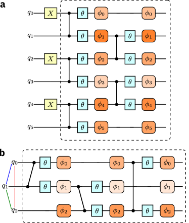
Fig. S1: Circuit model of Floquet dynamics. a. Gate schematic of initialization and one cycle of our Floquet model for an example of one-dimensional, 6-qubit lattice. All qubits are initialized to the target initial state using single-qubit $X$ gates applied to the initial all-zero state. The boxed area represents a single Floquet cycle, which is iterated to advance the dynamics of the system. b. Illustration of a single Floquet cycle in a two-dimensional lattice, showcasing three interconnected qubits. The colors of the connections on the left represent the sequential application of the two-qubit gates over their connectivity (i.e., graph coloring). Each layer consists two-qubit $CZ$ gates (depicted as black dots connected by lines), $U(\theta)$ gates shown as green boxes, and disorder gates $P(\phi_{i})$ depicted in orange. Visualizations were generated using Quantikz.

We always initiate the qubits in a product state in the computational basis. Since each product state is a superposition of many eigenstates of the unitary $U_{F}$, this circuit leads to far-from-equilibrium dynamics. The nature of this dynamics depends on the values of the angle $\theta$. As we will show numerically in the following section, in one dimension there exists a critical value of $\theta_{c}$ such that for $\theta<\theta_{c}$ the spectrum of the unitary $U_{F}$ behaves similarly to a set of random phases, while the eigenstates are low-entangled, signaling the presence of many-body localization (MBL). In contrast, for $\theta>\theta_{c}$ we observe signatures of chaotic dynamics, including a spectrum resembling a random matrix and high eigenstate entanglement.

More details about the circuit are in the Section II, including the implementation using native gates, simultaneous measurement of commuting observables, and error mitigation.

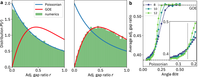
Fig. S2: Quasienergy level statistics for the one-dimensional (1D) circuits. a. The adjacent gap ratio distribution [see Eq. (S.5)] is depicted for the Floquet circuit at two different interaction $\theta$: $0.1\pi$ (left) and $0.3\pi$ (right). The left plot corresponds to the many-body localized (MBL) dynamical regime, while the right plot corresponds to the ergodic regime. The green-shaded bars display the distribution obtained over $10^{3}$ random disorder realizations of one-dimensional Floquet circuits with 12 qubits. The solid blue and red curves represent fits of the numerically-obtained distributions using Poissonian and Gaussian Orthogonal Ensemble (GOE) statistics, respectively. b. The transition from GOE to Poissonian statistics for different system sizes as shown by the average adjacent gap ratio for circuits containing from 8 to 12 qubits. The average is taken over $10^{3}$ individual circuits with different disorder realizations. The inset focuses on a crossover at $\theta\approx 0.16\pi$ (indicated by a vertical dotted line).

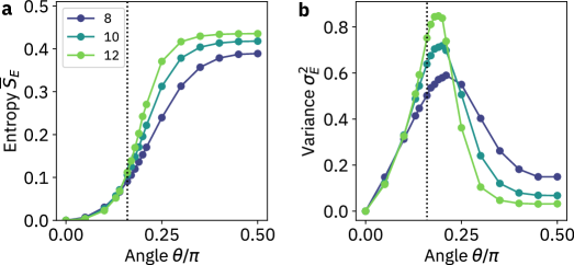
Fig. S3: Entanglement entropy for the one-dimensional (1D) circuits. a. The average entanglement entropy $\bar{S}_{E}$ of eigenstates per qubit across varying system sizes, as obtained from $10^{3}$ disorder realizations for 8-qubit circuits and $10^{2}$ realizations for 10- and 12-qubit circuits. The system demonstrates a crossover at $\theta\approx 0.16\pi$. b. The variance of entanglement entropy $\sigma_{E}^{2}$ among different eigenstates. This function has a pronounced peak that becomes sharper and converges to the critical point as system size increases.

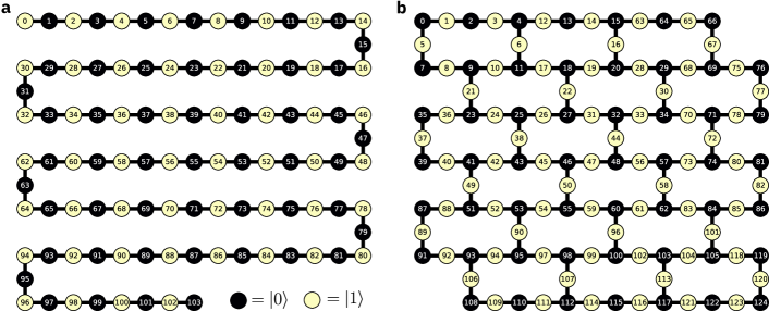
Fig. S4: Antiferromagnetic order of the initial states. The illustration displays the configuration for the initial states exhibiting antiferromagnetic order. Black circles represent qubits initialized in $|0\rangle$, while yellow those initialized in $|1\rangle$. a. Configuration used for the 1D chain comprising 104 qubits. b. Configuration of the 2D heavy-hexagon lattice, comprising 125 qubits.

I.2 Evidence of MBL regime

Here, we analyze the proposed model and demonstrate the existence of the MBL regime through numerical simulations performed on systems with 8 to 12 qubits.

A crucial characteristic of the MBL phase can be identified in the spectrum of the Floquet unitary. To show this, we examine the spectral decomposition

$$U_{F}|\alpha\rangle=\exp(i\lambda_{\alpha})|\alpha\rangle,$$ (S.4)

where $\lambda_{\alpha}\in[-\pi,\pi]$ are quasienergies and $|\alpha\rangle$ are corresponding eigenstates. Assuming that $\lambda_{\alpha}$ are set in increasing order, we define the spectral gaps as $\delta\lambda_{\alpha}=\lambda_{\alpha+1}-\lambda_{\alpha}.$ The main object we are interested in is adjacent gap ratios [pal2010mbl, zhang2016floquet] that can be defined as

$$r_{\alpha}=\frac{\min(\delta\lambda_{\alpha},\delta\lambda_{\alpha+1})}{\max(\delta\lambda_{\alpha},\delta\lambda_{\alpha+1})}.$$ (S.5)

The statistical distribution of $r_{\alpha}$ in the large system limit, denoted by $P(r_{\alpha})$, has different values in the ergodic and MBL phases. In particular, the MBL phase has Poisson level statistics, while the ergodic phase has the statistics of the Gaussian orthogonal ensemble (GOE) of matrices:

$$\begin{split}&P(r)=\frac{2}{(1+r)^{2}}\quad{\rm(Poisson)},\\ &P(r)=\frac{27}{4}\frac{r+r^{2}}{(1+r+r^{2})^{5/2}}\quad{\rm(GOE)}.\end{split}$$ (S.6)

The difference between these distributions can be used to distinguish the two regimes. The associated order parameter is the mean spectral gap ratio $\overline{r}=2^{-n}\sum_{\alpha}r_{\alpha}$. In the MBL phase, we expect this mean to reach the Poisson value $\overline{r}\approx 0.39$, while the GOE distribution for the ergodic phase has $\overline{r}\approx 0.53$ [pal2010mbl].

The spectral properties of our circuit are shown in Fig. S2a. Here we see that for $\theta=0.1\pi$ the level statistics almost perfectly follow the Poisson distribution. In contrast, for $\theta=0.3\pi$ it changes to the GOE distribution. This transition is illustrated for several circuit sizes in Fig. S2b. The curves show a strong crossover at $\theta_{c}\approx 0.16\pi$, indicating the presence of a transition between different level statistics. While the fate of this transition in the thermodynamic limit remains an open question [wdroeck2017stability, morningstar2022avalanches, sels2022avalanches], this critical value clearly distinguishes two dynamical regimes for small systems, which we refer to below as the “MBL regime” and the “ergodic regime”.

Another measure of localization is the bipartite entanglement entropy of the eigenstates of the Floquet unitary. To define it, we divide the system into two equal parts and label them as subsystem $A$ and subsystem $B$. Then we can represent each eigenstate $|\alpha\rangle$ using Schmidt decomposition

$$|\alpha\rangle=\sum_{\mu}\eta_{\alpha\mu}|\psi^{A}_{\mu\alpha}\rangle\otimes|\psi^{B}_{\mu\alpha}\rangle,$$ (S.7)

where $|\psi^{A}_{\mu\alpha}\rangle$ and $|\psi^{B}_{\mu\alpha}\rangle$ are some basis states of the subsystems $A$ and $B$, respectively. The entropy of bipartite entanglement is defined as

$$S_{\alpha}:=-\sum_{\mu}\eta^{2}_{\alpha\mu}\log_{2}\eta^{2}_{\alpha\mu}.$$ (S.8)

As an associated order parameter we use the average entanglement entropy per qubit,

$$\overline{S}_{E}:=\frac{1}{2^{n}n}\sum_{\alpha}S_{\alpha}.$$ (S.9)

For the MBL phase, we expect the entanglement entropy to exhibit an area law, i.e. it remains constant independent of the number of qubits $n$ [pal2010mbl]. This means that in the MBL phase it has scaling $\overline{S}_{E}=O(n^{-1})$. In contrast, in the ergodic phase Floquet dynamics thermalizes the subsystems to local infinite temperature. In this state the entropy saturates at the Page value,

$$\overline{S}_{E}\simeq\frac{1}{2}-\frac{1}{2n\ln 2}+O\left(2^{-n}\right).$$ (S.10)

Thus it saturates to a constant in the large system limit. Another test of the MBL phase transition is the variance of the entanglement distribution over eigenstates, i.e.

$$\sigma^{2}_{E}:=\frac{1}{2^{n}}\sum_{\alpha}(S_{\alpha}-\overline{S})^{2}.$$ (S.11)

The maximum of the variance $\sigma_{S}$ indicates the point of the phase transition for $n\gg 1$.

The entanglement entropy for the Floquet unitary is depicted in Fig. S3. Similar to the level statistics, the entropy per qubit exhibits distinct behaviors on opposite sides of the critical point $\theta_{c}\approx 0.16\pi$ as the system size increases. Notably, in the MBL regime, its value displays a gradual decline with increasing of the system size, whereas in the ergodic regime, it ascends towards the Page value. The entropy variance also has a pronounced peak near the transition point, which lends further support to the existence of an MBL regime and its transition into ergodic behavior in our system.

We do not present the evaluation of level statistics or entanglement entropy for two-dimensional systems as it technically challenging due to the exponential overhead in classical complexity. Consequently, it remains uncertain whether the regime we observe for low $\theta$ values exhibits characteristic features of MBL. We nonetheless refer to it as the “prethermal regime” for simplicity, predicated on the assumption that localization signatures should persist in small two-dimensional systems at shallow depths. Our study does, however, highlight a significant disparity between the dynamics of one- and two-dimensional systems when viewed from the lens of the spectrum of the one-particle density matrix, as depicted in Fig. 2d and Fig. 4d (definition provided below). It is worth noting that this observed effect could potentially be a consequence of noise – a hypothesis that can be confirmed in future studies with higher-fidelity quantum hardware.

I.3 Spin imbalance

Unlike level statistics or entanglement entropy, the spin imbalance – defined in the following paragraph – is a localization measure that can be efficiently determined on real hardware without the exponential sampling overhead. Its detection involves the preparation of a structured initial state and the measurement of a certain parameter that describes its local order. In the MBL regime, the order parameter is expected to never decrease below a certain value, since the local memory of the initial state persists over time. Conversely, in the ergodic phase, the local order dissipates rapidly, rendering the initial state irretrievable.

A commonly used ordered state is the antiferromagnetic ordered state (previous works also use the terms “antiferromagnetic” or “Néel state”). Its layout in one dimension is illustrated in Fig. S4a. To define the order parameter, we group all qubits into set $S_{0}$, which contains all qubits initialized in state $|0\rangle$, and set $S_{1}$ containing the qubits initialized in state $|1\rangle$. Then we define the spin imbalance at Floquet cycle $d$ as

$$\mathcal{I}_{d}=\frac{n_{d1}-n_{d0}}{n_{d1}+n_{d0}},$$ (S.12)

where the average population $n_{dk}$ of the qubits in the set $S_{k}$ with size $N_{k}$ takes the form

$$n_{dk}=\frac{1}{2}-\frac{1}{2N_{k}}\sum_{i\in S_{k}}\langle\psi_{d}|Z_{i}|\psi_{d}\rangle,\quad|\psi_{d}\rangle=U_{F}^{d}|\psi_{0}\rangle.$$ (S.13)

In two dimension s, the choice of the ordered state has more freedom. We choose the antiferromagnetic state shown in Fig. S4b, where the nearest neighbors are always in different states. Note, however, that this configuration has a larger number $N_{1}$ of $|1\rangle$ states than the number $N_{0}$ of $|0\rangle$ states.

The spin imbalance renormalized to compensate for the effect of noise is shown in Figs. 2b and 4c. The details of the renormalization and further experimental data are given in Sec. III below.

I.4 One-particle density matrices (OPDMs)

Here, we study the one-particle density matrix (OPDM), an $n\times n$ matrix with its elements defined for an arbitrary multi-qubit state $|\psi\rangle$ as

$$\rho_{ij}=\langle\psi|a_{i}^{\dagger}a_{j}|\psi\rangle-\langle\psi|a_{i}^{\dagger}|\psi\rangle\langle\psi|a_{j}|\psi\rangle,$$ (S.14)

where we denote the Fock operator for hardcore bosons $a_{i}=\frac{1}{2}(X_{i}-iY_{i})$.

We can study the spectrum of the OPDM through the eigenproblem

$$\rho|\varphi_{k}\rangle=\nu_{k}|\varphi_{k}\rangle,$$ (S.15)

where $|\varphi_{k}\rangle$ are natural orbitals and $\nu_{k}$ are ordered occupation numbers, $\nu_{k+1}\geq\nu_{k}$. In the case of a Gaussian state of fermions or hardcore bosons, the OPDM offers a comprehensive description of the system. The state of the system can be seen as a collection of one-particle orbitals $|\varphi_{k}\rangle$ occupied with probabilities $\nu_{k}\in\{0,1\}$. For other many-body states, this description extends to a probabilistic mixture of quasiparticle states occupying orbitals with probabilities $\nu_{k}$ [bera2015opdm, bera2017opdm]. The conservation of occupation numbers serves as a robust indicator of the stability of quasiparticles [mahan2000many].

We evaluate OPDM for late-time state $|\psi_{D}\rangle$ with the initial state of the system $|\psi_{0}\rangle$ set to the CDW state described in the previous section. As an order parameter, we use the discontinuity parameter

$$\delta=\left\langle\nu_{N_{0}+1}-\nu_{N_{0}}\right\rangle_{\rm dis},$$ (S.16)

where $\langle\dots\rangle_{\rm dis}$ is the disorder average. The the subscripts $N_{0}$ indicates number of qubits prepared in the zero state. In the initial CDW state, the value of the discontinuity is $\delta=1$. For ergodic systems in both the thermodynamic and large-depth limits $D\to\infty$, the discontinuity vanishes, $\lim_{D\to\infty}\delta\to 0$, as the system loses all local memory of the initial state and the diagonalized OPDM becomes proportional to identity matrix. In contrast, in the MBL regime, the discontinuity saturates at a constant value $\lim_{D\to\infty}\delta>0$ due to the presence of stable quasiparticles. For finite systems and restricted depth $D$, we can use finite-size analysis of the discontinuity to detect the presence of a phase transition, as we show in Fig. 2c and d.

I.5 Local integrals of motion (LIOMs)

The central topic of our study are integrals of motion, which we denote by symbol $L$. In particular, we aim to find a set of real coefficients $\{a_{\mu}\}$ such that the operator

$$L=\sum_{\mu=1}^{4^{n}-1}a_{\mu}P_{\mu}$$ (S.17)

is conserved, i.e. $[L,U_{F}]=0$, where $P_{\mu}$ denote all possible generalized Pauli operators except the identity (e.g., for 4 qubits this set would include, for example, the operators like $XIZY$ or $IIXZ$ but not $IIII$).

In a quantum system comprising $n$ qubits, there exist precisely $2^{n}$ independent integrals of motion. One possible choice of these operators is the ket-bra set $\{|\alpha\rangle\langle\alpha|\}$, where $|\alpha\rangle$ are the eigenstates of the Floquet unitary. It is crucial to highlight that these integrals of motion are nonlocal, signifying that they depend on Pauli matrices $P_{\mu}$ acting on most of the qubits. However, for certain integrable systems, sets of integrals of motion can be derived from a closed set of local conserved operators. As an example, a unitary classical spin system exhibits a set of Pauli operators $Z_{k}$ that commute with the unitary evolution operator. These operators can be summed and multiplied between each other to generate arbitrary sets of conserved operators.

In this context, the MBL phase can be understood similarly to a classical spin system [serbyn2013lioms, huse2014lioms]. In particular, there are $n$ local integrals of motion (LIOMs), similar to $Z_{k}$. Unlike classical systems, however, they are not diagonal and act on many qubits. For these LIOMs, the coefficients follow an empirical bound

$$|a_{\mu}|\leq\exp(-(|P_{\mu}|+d_{\mu})/\xi),$$ (S.18)

where $|P_{\mu}|$ is a full support of the Pauli matrix $P_{\mu}$, $d_{\mu}$ is the distance between the central qubit of the LIOM and the center of the operator $P_{\mu}$, and $\xi$ is the localization length. By full support here we mean the size of the smallest continuous subset $P_{\mu}$ acts on non-trivially. For example, in one dimension, both $IIYZZ$ and $IXIZI$ have support 3. By the center of the operator $P_{\mu}$ we mean the geometrical center that the subset is supported on, or qubits 3 and 2 (assuming zero-indexing), respectively, in the two previous examples.

Due the method’s error and effect of noise, obtained LIOMs will be approximate, with deviation quantified as

$$\epsilon:=\frac{\|[U_{F},L]\|_{F}}{2\|L\|_{F}}.$$ (S.19)

This quantity is bounded as $0\leq\epsilon\leq 1$ and vanishes when $[U_{F},L]=0$. The numerator and denominator of this expression are given by

$$\begin{split}&\|[U_{F},L]\|_{F}^{2}=2^{n+2}\sum_{\mu\nu}a_{\mu}B_{\mu\nu}a_{\nu},\\ &\|L\|_{F}^{2}=2^{n}\sum_{\mu}a_{\mu}^{2},\end{split}$$ (S.20)

where we defined the matrix of the connected single cycle time correlation function for two Pauli operators as

$$B_{\mu\nu}=\frac{1}{2}\Bigl{(}-\frac{1}{2^{n}}{\rm Tr\,}(U_{F}^{\dagger}P_{\mu}U_{F}P_{\nu})+\delta_{\mu\nu}\Bigl{)}.$$ (S.21)

To avoid confusion with other errors, we refer to $\epsilon$ as LIOM imprecision throughout the main text and subsequent sections. Using the matrix $B$, we can express the LIOM imprecision as

$$\epsilon=\Biggl{[}\frac{\sum_{\mu\nu}a_{\mu}B_{\mu\nu}a_{\nu}}{\sum_{\mu}a_{\mu}^{2}}\Biggl{]}^{1/2}\equiv\sqrt{\tilde{a}^{T}B\tilde{a}},$$ (S.22)

where $\tilde{a}=\{\tilde{a}_{\mu}\}$ represents the vector of normalized coefficients $\tilde{a}_{\mu}=a_{\mu}/\sqrt{\sum_{\mu}a_{\mu}^{2}}$.

Let us evaluate the imprecision $\epsilon_{0}$ for the one-dimensional circuit using $L\equiv Z_{i}$, where $i\neq 1,n$. To do this, we note that

$$\begin{split}\epsilon_{0}&=\frac{1}{2^{n/2+1}}\|[U_{F},Z_{i}]\|_{F}\\ &=\frac{1}{2^{n/2+1}}\|C^{Z}_{i,i+s}U_{i}(\theta)Z_{i}U_{i}(\theta)C^{Z}_{i,i+s}\\ &\qquad\qquad-P^{\dagger}(\phi_{i})U_{i}(\theta)Z_{i}U_{i}(\theta)P(\phi_{i})\|_{F},\end{split}$$ (S.23)

where $s=+1$ for even $i$ and $s=-1$ for odd $i$. Here, we used the Floquet unitary decomposition in Eqs. (S.2) and (S.3) and the fact that the Frobenius norm is invariant to multiplication of the operator by unitary either from the left or from the right. The operator terms inside the norm can be expressed as

$$\begin{split}&C^{Z}_{i,i+s}U_{i}(\theta)Z_{i}U_{i}(\theta)C^{Z}_{i,i+s}=Z_{i}\cos\theta+X_{i}Z_{i+s}\sin\theta\\ &P^{\dagger}(\phi_{i})U_{i}(\theta)Z_{i}U_{i}(\theta)P(\phi_{i})=Z_{i}\cos\theta+X_{i}\sin\theta\cos\phi_{i}\\ &\qquad\qquad\qquad\qquad\qquad\qquad\qquad\qquad+Y_{i}\sin\theta\sin\phi_{i}.\end{split}$$ (S.24)

As the result, we have

$$\begin{split}\epsilon_{0}&=\frac{\sin\theta}{2^{n/2+1}}\|X_{i}Z_{i+s}-X_{i}\cos\phi_{i}-Y_{i}\sin\phi_{i}\|_{F}=\frac{\sin\theta}{\sqrt{2}}.\end{split}$$ (S.25)

This result does not depend on $\phi_{i}$ and thus on the disorder realization or the qubit position (except for the first and the last qubit we did not consider above). The value of $\epsilon_{0}$ is shown as a dashed red line in Fig. 3e for $\theta=0.1\pi$.

The following sections describe the process of generating LIOMs. This process depends on an initial guess. The accuracy of this initial guess is not critical, but an improved estimate is expected to lead to better convergence. We then present two strategies for formulating this initial estimate: one based solely on theoretical analysis and the other based solely on experimental data. Finally, we examine the convergence of our approach and its limitations, in particular those induced by the presence of noise.

I.6 Generating LIOMs via time averaging

Given an initial guess $L^{(0)}$, we derive the corresponding approximate LIOM using the expression

$$L^{(D)}=\mathbb{E}_{d\leq D}\left[\mathcal{E}^{d}_{F}(L^{(0)})\right],$$ (S.26)

where the inverse-time Floquet cycle map $\mathcal{E}_{F}(\cdot)$ and its average $\mathbb{E}_{d\leq D}$ over cycles $0$ to $D$ cycles are defined as

$$\begin{split}&\mathcal{E}_{F}(O):=U_{F}OU_{F}^{\dagger},\\ &\mathbb{E}_{d\leq D}[O_{d}]:=\frac{1}{D+1}\sum_{d=0}^{D}O_{d},\end{split}$$ (S.27)

where $\{O_{d}\}$ is an arbitrary sequence of $D$ operators. Note that in the inverse time the order of the operator $U_{F}$ and the conjugate operator $U_{F}^{\dagger}$ is reversed compared to the forward time evolution of operators in the Heisenberg picture (or in the order corresponding to a density matrix). This order is chosen so that it is convenient to express $L^{(D)}$ below in terms of the evolution of the eigenstates of the operator $L^{(0)}$. This operator becomes an exact LIOM in the limit $D\to\infty$, i.e. $[L^{(\infty)},U_{F}]=0$. Indeed,

$$U_{F}L^{(\infty)}U^{\dagger}_{F}=\lim_{D\to\infty}\frac{1}{D+1}\sum_{d=0}^{D}U^{d+1}_{F}L^{(0)}U^{d+1{\dagger}}_{F}=L^{(\infty)}.$$ (S.28)

In the following section, we explore the convergence of this method for finite $D$ (see Proposition 1).

The Pauli coefficients of the operator in Eq. (S.26) are

$$\begin{split}a_{\mu}&=\frac{1}{2^{n}}{\rm Tr\,}(P_{\mu}L^{(D)})\\ &=\frac{1}{2^{n}}\frac{1}{D}\sum_{d=0}^{D-1}{\rm Tr\,}(U^{d{\dagger}}_{F}P_{\mu}U^{d}_{F}L^{(0)})\equiv\frac{1}{D}\sum_{d=0}^{D-1}W_{d}(P_{\mu},L^{(0)}),\\ \end{split}$$ (S.29)

which leads us to Eq. (3) in the main text in the limit $D\to\infty$. Here, we used the notation

$$W_{d}(P_{\mu},L^{(0)})=\frac{1}{2^{n}}{\rm Tr\,}(U^{d{\dagger}}_{F}P_{\mu}U^{d}_{F}L^{(0)}).$$ (S.30)

As the first step for evaluating the trace in Eq. (S.29), we use the spectral decomposition of the inital guess operator $L^{(0)}$ as

$$L^{(0)}=\sum_{\alpha=1}^{2^{n}}p_{\alpha}|\psi_{\alpha}\rangle\langle\psi_{\alpha}|,$$ (S.31)

where $p_{\alpha}$ and $|\psi_{\alpha}\rangle$ are corresponding eigenvalues and eigenstates. This expression leads us to

$$\begin{split}W_{d}(P_{\mu},L^{(0)})=\frac{1}{2^{n}}\sum_{\alpha=1}^{2^{n}}p_{\alpha}\langle\psi_{\alpha}|U_{F}^{d{\dagger}}P_{\mu}U^{d}_{F}|\psi_{\alpha}\rangle.\end{split}$$ (S.32)

If we choose $L^{(0)}$ to be an operator in the computational basis, one could approximate the coefficients using a sum over a limited subset of bitstrings $\mathcal{S}$, which size $|\mathcal{S}|$ can be small. (Although one could use Monte Carlo sampling of these bitstrings, in the next section, we propose a more efficient method that is also suitable for shallow circuits.) Thus we get

$$W_{d}(P_{\mu},L^{(0)})\approx\frac{1}{|\mathcal{S}|}\sum_{\alpha\in|\mathcal{S}|}p_{\alpha}\langle\psi_{\alpha}|U_{F}^{d{\dagger}}P_{\mu}U^{d}_{F}|\psi_{\alpha}\rangle.$$ (S.33)

An advantage of this method is that it allows us to obtain the coefficients $a_{\mu}$ individually, without accessing the whole operator $L$. Therefore, we can learn some properties of $L$ without running out of classical memory to keep its full representation. This is useful when the system is close to the critical point where the correlation length $\xi$ in Eq. (S.18) is large, leading to a significant number of relevant coefficients $a_{\mu}$ that grows exponentially with $\xi$. Another advantage of this method is that the noise may partially self-average as a result of summing over many Floquet cycles in Eq. (S.29).

In the literature, it is often considered a set of LIOMs that are orthonormal with respect to inner products and do not retain the properties of Pauli operators. Such operators are commonly called logical bits or “l-bits”. Our operators do not have such properties, but one could obtain the set of l-bits by classical postprocessing using a nonlinear transformation of the obtained LIOMS.

I.7 Choosing the initial guess

In this section, we present and discuss several strategies for selecting operators that can serve as initial guesses. The first strategy is the straightforward selection of Pauli $Z$ operators. The second strategy requires an understanding of the $U_{F}$ structure of the Floquet unitary and aims at minimizing the norm of the commutator $[U_{F},L]$. The third strategy extracts the initial estimate from experimental data and reduces the variance of the operator $L^{(0)}$ throughout its time evolution. Both theoretical and experimental optimization strategies are not perfect as standalone LIOM discovery methods due to their lack of scalability: they require a complete classical representation of the LIOM. However, we believe they are adequate for making an initial guess as we can limit our considerations to LIOMs with a support that meets available computational resources. In the following, we discuss each of these strategies in further detail.

Strategy 1: a simple guess. Since the system is strongly disordered in the z-direction, it is reasonable to assume that the operators $Z_{i}$ for $i=1,\dots,n$ represent a good option for the initial guess,

$$L^{(0)}\in\{Z_{i}\}.$$ (S.34)

Due to the depth limitations ($D\sim 10$) given the existing level of noise (see next section), we found this choice to be the best at illustrating the capability of quantum hardware to converge to better LIOMs. This is why it is used in the main text. However, we also explored other options that could generate even better initial guess values. Below we list two such methods that may be useful for deeper circuits.

Strategy 2: theoretical optimization. Let us assume that we have an access to the full Floquet unitary. We are looking for our guess in the form

$$L^{(0)}=\sum_{\mu\in Q}a_{\mu 0}P_{\mu},\qquad\sum_{\mu}a^{2}_{\mu 0}=1,$$ (S.35)

where $Q$ is a certain subset of Pauli operators with number $q$ of $k$-local Pauli operators. It is also beneficial to choose only Pauli operators in the computational basis to reduce the computational resources required to obtain full LIOMs, as we describe further in the following section.

Next, our goal is to minimize the error

$$\epsilon_{0}:=\frac{\|[U_{F},L^{(0)}]\|_{F}}{2\|L^{(0)}\|_{F}}=\sqrt{a_{0}^{T}Ba_{0}},$$ (S.36)

where $a_{0}=\{a_{\mu 0},0\dots 0\}$ is the vector where all coefficient for Pauli operators in $Q$ are replaced by $a_{\mu 0}$, and the rest of elements are zero. This can be done by solving the eigenproblem for the matrix in Eq. (S.21),

$$\sum_{\nu\in Q}B_{\mu\nu}a_{\nu 0}=b_{0}a_{\mu 0}$$ (S.37)

for the smallest eigenvalues $b_{0}$. The minimum error is $\epsilon=\sqrt{b_{0}}$. Because vector $a_{0}$ has only $q$ non-zero entrees, we need evaluate only a block of size $q\times q$ corresponding to nonzero $a_{\mu 0}$, not the entire matrix $B$.

Strategy 3: experimental optimization. Consider $\Psi=\{|\psi_{0}^{(k)}\rangle\}$ to be a set of initial states and $Q$ is the set of Pauli matrices supported on a certain subset of qubits. Using the decomposition in Eq. (S.35), we rewrite the expectation value of the evolved initial guess as

$$\begin{split}\langle\psi_{0}^{(k)}|U_{F}^{d{\dagger}}L^{(0)}U_{F}^{d}|\psi_{0}^{(k)}\rangle=\sum_{\mu\in\mathcal{S}}a_{\mu 0}f_{\mu kd},\end{split}$$ (S.38)

where the coefficients $f_{\mu km}$ are the expectation values for Pauli operator $P_{\mu}$ after $n$ cycles of evolution for the $k$-th initial state, i.e.

$$f_{\mu kd}:=\langle\psi_{0}^{(k)}|U_{F}^{{\dagger}d}P_{\mu}U_{F}^{d}|\psi_{0}^{(k)}\rangle.$$ (S.39)

Then, the coefficients for an approximate LIOM can be found by minimizing the variation

$$\{a_{\mu 0}\}={\rm argmin}\,\sum_{k}{\rm Var}_{d\leq D}\Bigl{(}\sum_{\mu\in Q}a_{\mu 0}f_{\mu kd}\Bigl{)},$$ (S.40)

where ${\rm Var}_{d\leq D}[O_{d}]:=\mathbb{E}_{d\leq D}[O^{2}_{d}]-(E_{d\leq D}[O_{d}])^{2}$. In general, the maximum circuit depth $D$ and set size $|\Psi|$ must satisfy $D|\Psi|\geq q$ to avoid overfitting. Notably, this method can be implemented even for shallow circuits. Technically, for noiseless circuits, depth $D=1$ is sufficient if the set $\Psi$ is large enough.

The optimal values of $a_{\mu 0}$ can be found by solving the spectral problem

$$A_{\mu\nu}a_{\nu 0}=wa_{\mu 0},$$ (S.41)

for smallest possible $w$, where the matrix $A$ is generated as

$$\begin{split}A_{\mu\nu}=\sum_{k}\Bigl{(}\mathbb{E}_{d\leq D}&[f_{\mu kd}f_{\nu kd}]\\ &-\mathbb{E}_{d\leq D}[f_{\mu kd}]\mathbb{E}_{d^{\prime}\leq D}[f_{\nu kd^{\prime}}]\Bigl{)}.\end{split}$$ (S.42)

Both strategy 2 and strategy 3 are not scalable because they require classical storage and processing of all $a_{\mu 0}$ that define the LIOM. This number grows exponentially with the support of LIOMs and quickly becomes intractable, especially near the phase transition point. However, by truncating the support, these methods can be used to find a good initial guess.

I.8 Convergence and noise

This section focuses on evaluating the performance of the proposed method under noise constraints. First, we postulate two essential properties of the studied quantum dynamics. These properties are then used to derive two error bounds: with respect to finite depth and with respect to noise. By combining these error estimates, we determine the optimal circuit depth for the experiment.

The first property concerns the conservation of local operators. In the MBL regime, the values of most of the local operators are partially conserved due to their overlap with LIOMs. A formal statement of memory preservation can be expressed by an inequality applied to local operators $O$,

$${\rm Tr\,}(U_{F}^{d{\dagger}}OU_{F}^{d}O)\geq\lambda_{d}(O)\|O\|_{F}^{2},$$ (S.43)

where $\|\cdot\|_{F}$ is the Frobenius norm, $\lambda_{d}(O)\geq 0$ is an operator-specific memory parameter that remains constant or decreases monotonically with increasing depth $d$. In the MBL phase, we expect the parameter to remain nonzero, i.e. $\lim_{d\to\infty}\lambda_{d}(O)>0$. If the system is egodic, we expect $\lambda_{d}(O)\gtrsim\exp(-d/D_{\rm th})$ for local operators, where $D_{\rm th}$ is the thermalization time scale. The term “prethermal” refers to a regime in which thermalization proceeds at a very slow rate, such that $D_{\rm th}\gg D$. In other words, the thermalization time scale is much larger than the number of observation cycles $D$.

The second property is localization. For all systems, including localized ones, there is a Lieb-Robinson bound that limits the instantaneous propagation of information for large distances. For the MBL phase, this bound can be expressed in a stronger, “logarithmic” form [burrell2007bounds],

$$\|[U_{F}^{d{\dagger}}O_{1}U_{F}^{d},O_{2}]\|\leq c\|O_{1}\|\|O_{2}\|d^{\alpha}e^{-{\rm dis}(O_{1},O_{2})/\xi_{0}},$$ (S.44)

where $\|\cdot\|$ is the operator norm, ${\rm dis}(O_{1},O_{2})$ is the distance between the operators $O_{1}$ and $O_{2}$, $\xi_{0}$ is the localization length, $c$ is a contant, and $\alpha>0$ is the exponent. For slowly thermalizing ergodic systems, we expect this inequality to hold empirically if we replace the constant localization length by a slowly changing cycle-dependent one, $\xi_{0}\to\xi_{d}$. We further assume that the localization length grows very slowly with cycle number $d$, so that its change remains negligible within $D_{\rm th}$ cycles.

Using the first property, we can show that as the maximum cycle depth $D$ grows, the method progressively converges to the target LIOM.

Proposition 1 (Depth convergence).

For any Floquet dynamics satisfying Eq. (S.43), the imprecision of the operator in Eq. (S.26) is bounded as

$$\epsilon:=\frac{\|[L^{(D)},U_{F}]\|_{F}}{2\|L^{(D)}\|_{F}}\leq\frac{1}{\sqrt{\lambda_{D}(L^{(0)})}D}.$$ (S.45)

Proof.

First, we rewrite the commutator as

$$\begin{split}[U_{F},L^{(D)}]&=\Bigl{(}U_{F}L^{(D)}U^{\dagger}_{F}-L^{(D)}\Bigl{)}U_{F}\\ &=\frac{1}{D}\Bigl{(}U_{F}^{d+1}L^{(0)}U^{d+1{\dagger}}_{F}-L^{(0)}\Bigl{)}U_{F}.\end{split}$$ (S.46)

Next, using the invariance of the Frobenius norm under rotations as well as the triangle inequality, we derive that

$$\begin{split}\|[U_{F},L^{(D)}]\|_{F}&=\frac{1}{D}\Bigl{\|}\mathbb{E}_{d\leq D}\Bigl{(}U_{F}^{d+1}L^{(0)}U^{d+1{\dagger}}_{F}-L^{(0)}\Bigl{)}U_{F}\Bigl{\|}_{F}\\ &=\frac{1}{D}\Bigl{\|}\mathbb{E}_{d\leq D}U_{F}^{d+1}L^{(0)}U^{d+1{\dagger}}_{F}-L^{(0)}\Bigl{\|}_{F}\\ &\leq\frac{2}{D}\|L^{(0)}\|_{F}.\end{split}$$ (S.47)

Finally, we rewrite the norm of the operator $L^{(D)}$ using its definition as

$$\begin{split}\|L^{(D)}\|_{F}&\equiv\sqrt{{\rm Tr\,}(L^{(D)2})}\\ &=\sqrt{\mathbb{E}_{d\leq D}{\rm Tr\,}\Bigl{(}U_{F}^{d}L^{(0)}U_{F}^{d{\dagger}}L^{(0)}\Bigr{)}}\\ &\geq\sqrt{\lambda_{D}(L^{(0)})}\|L^{(0)}\|_{F},\end{split}$$ (S.48)

where in the last step we used Eq. (S.43). By inserting Eq. (S.47) and (S.48) into Eq. (S.45) we get the desired result. This step completes our proof. ∎

Note that the right-hand side of the Eq. (S.45) depends on $\lambda_{D}(L^{(0)})$. This implies that an accurate initial guess, denoted by $L^{(0)}$, can significantly improve the efficiency of the procedure. In particular, increasing the value of $\lambda_{D}(L^{(0)})$ will reduce the corresponding error. Thus, the selection of a better initial guess for $L^{(0)}$ is crucial to minimize the error and improve the overall accuracy and efficiency of the method. We also expect $\lambda_{D}(L^{(0)})$ to decrease exponentially with the localization length $\xi_{0}$. Thus, systems with smaller localization lengths should show significantly faster convergence.

Improvements made by increasing depth are limited by the effects of noise. Two primary categories of noise affect the system: systematic and stochastic. Systematic noise comes from calibration and readout errors. Predicting the influence of this type of noise is particularly challenging because it is hardware-dependent and can vary subtly over time. However, its impact is most noticeable for a few “problematic” qubits and/or qubit coupling, see Fig. S6. For the majority of qubits, the main source of error is stochastic noise.

We consider a simplistic noise model where we assume that after each Floquet cycle the qubits are subjected to a single-qubit depolarizing channel. In this context, the unitary transformation $\mathcal{E}_{F}$ previously described in Eq. (S.27) must be replaced by its noisy version, which has the form

$$\mathcal{E}^{\prime}_{F}:=\prod_{r=1}^{n}\Bigl{(}(1-p)\hat{I}+\frac{p}{3}\sum_{ar}\Lambda_{ar}\Bigl{)}\mathcal{E}_{F},$$ (S.49)

where $p$ is the error probability, $\hat{I}$ is the identity superoperator, and $\Lambda_{ar}$ is a single-qubit Pauli channel.

$$\Lambda_{ar}(\cdot):=P_{ar}(\cdot)P_{ar},$$ (S.50)

and $P_{ar}\in\{X_{r},Y_{r},Z_{r}\}$ are single-qubit Pauli operators.

Consequently, the outcome obtained from the experimental data corresponds is the modified approximate LIOM $\tilde{L}^{(D)}$ that takes the form

$$\tilde{L}^{(D)}=\mathbb{E}_{d\leq D}\mathcal{E}^{\prime d}_{F}(L^{(0)}).$$ (S.51)

To establish the effect of the noise, we prove the following Proposition.

Proposition 2.

For any noiseless dynamics satisfying (S.44), the noisy dynamics in Eq. (S.49) has the action

$$\mathcal{E}^{\prime d}_{F}(L^{(0)})=\mathcal{E}^{d}_{F}(L^{(0)})+\delta C_{d},$$ (S.52)

where the correction operator $\delta C_{d}$ satisfies

$$\frac{\|\delta C_{d}\|}{\|L^{(0)}\|}\leq cpd\sum_{r}\exp(-\Delta_{r}(L^{(0)})/\xi_{d}),$$ (S.53)

and $\Delta_{r}$ is the lattice distance between the qubit $r$ and the support of operator $L^{(0)}$.

Proof.

We start by stochastically decomposing the noisy evolution superoperator as

$$\begin{split}\mathcal{E}_{F}^{\prime d}&=\sum_{\bm{r}\bm{a}\bm{d}}p_{\bm{r}\bm{a}\bm{d}}\mathcal{E}_{F}^{d-d_{1}}\Lambda_{a_{1}r_{1}}\mathcal{E}_{F}^{d_{1}-d_{2}}\Lambda_{a_{2}r_{2}}\dots\Lambda_{a_{k}r_{k}}\mathcal{E}_{F}^{d_{k}}\\ &=\mathcal{E}_{F}^{d}\sum_{\bm{r}\bm{a}\bm{d}}p_{\bm{r}\bm{a}\bm{d}}\Lambda^{(d_{1})}_{a_{1}r_{1}}\Lambda^{(d_{2})}_{a_{2}r_{2}}\dots\Lambda^{(d_{k})}_{a_{k}r_{k}},\end{split}$$ (S.54)

where $p_{\bm{r}\bm{a}\bm{m}}=(1-p)^{nd-k}(p/3)^{k}$ represents the probability of a combination of $0\leq k\leq nd$ single-qubit Pauli errors $\bm{a}=\{a_{1},\dots,a_{k}\}$ involving qubits $\bm{r}=\{r_{1},\dots,r_{k}\}$ at cycle depths $\bm{d}=\{d_{1},\dots,d_{k}\}$. Here we have introduced the time-renormalized unitary error channels as

$$\Lambda_{ar}^{(d)}(\cdot):=\mathcal{E}_{F}^{{\dagger}d}\Lambda_{ar}\mathcal{E}_{F}^{d}=V_{ar}^{(d)}(\cdot)V_{ar}^{(d){\dagger}},$$ (S.55)

where we use the notation

$$V_{ar}^{(d)}:=U_{F}^{{\dagger}d}P_{ar}U_{F}^{d}$$ (S.56)

and $P_{ar}\in\{X_{r},Y_{r},Z_{r}\}$ is single-qubit Pauli operator acting on qubit $r$.

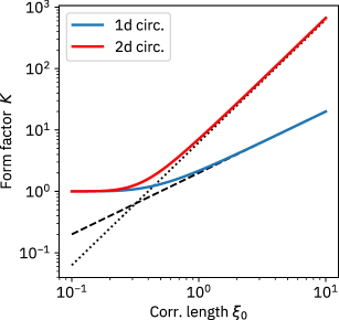
Fig. S5: Noise form factor. Form factor $K$ as a function of correlation length $\xi_{0}$ for $c=1$. The blue curve shows $K$ for infinite one-dimensional circuits, while the red curve shows a similar dependence for two-dimensional heavy-hexagonal circuits. The dashed curve shows the asymptotics $K=2\xi_{0}$ and the dotted curve shows $K=2\pi\xi_{0}^{2}$. The support of the operator $L^{(0)}$ in the two-dimensional case is a qubit with three neighbors (the case of two-neighbor qubit is very similar and is not shown).

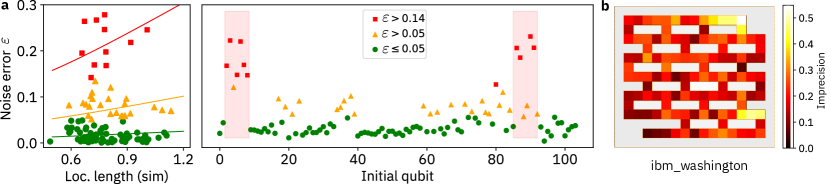
Fig. S6: Local integrals of motion (LIOMs) error due to noise. a. Noise error for 1D experiment. The plot shows the deviation of the coefficients $\bm{a}=\{a_{\mu}\}$ in Eq. (S.29) obtained experimentally from the same coefficients $\bm{a}_{\rm sim}$ obtained by noiseless simulation, as quantified by the noise error $\varepsilon=\|\bm{a}-\bm{a}_{\rm sim}\|_{2}/\|\bm{a}_{\rm sim}\|_{2}$. For illustration, the LIOMs are divided into three groups: low precision (red, $\varepsilon>0.14$), medium precision (orange, $0.05<\varepsilon\leq 0.14$), and high precision (green, $\varepsilon\leq 0.05$). Left panel shows the distribution of LIOMs as a function of their localization length (derived from simulations). The panel shows that low- and high-precision LIOMs have similar localization lengths. Solid lines represent the theoretical estimate for $\varepsilon$ in Eq. (S.70) for $p/\sqrt{\lambda_{0}}=10^{-3}$ (green), $4\cdot 10^{-2}$ (orange) and $1.2\cdot 10^{-2}$ (red). The right panel shows the dependence of the error on the position of the initial guess $L^{(0)}$. This panel shows that the high errors are clustered around certain regions (shaded by red), suggesting that high errors are generated by a few “bad” qubits or connections. b. LIOM imprecision for a 2D experiment. Each qubit $i$ is assigned a value of LIOM imprecision associated with the initial guess $L^{(0)}=Z_{i}$. Values are displayed in a 2D grid where neighboring cells correspond to neighboring qubits. As in 1D, anomalous values of imprecision are concentrated in a few regions.

Next, we rewrite the action of $d$ cycles of noisy evolution as in Eq. (S.52), where we introduce the correction operator as

$$\begin{split}\delta C_{m}=\mathcal{E}_{F}^{m}\sum_{\bm{r}\bm{a}\bm{m}}p_{\bm{r}\bm{a}\bm{m}}\Bigl{(}\Lambda^{(d_{1})}_{a_{1}r_{1}}\Lambda^{(d_{2})}_{a_{2}r_{2}}\dots\Lambda^{(d_{k})}_{a_{k}r_{k}}(L^{(0)})-L^{(0)}\Bigl{)}.\end{split}$$ (S.57)

Taking the Frobenius norm of this operator and using the fact that it is invariant under unitary transformations $\mathcal{E}_{F}$, we get

$$\begin{split}\|\delta C\|&\leq\sum_{\bm{r}\bm{a}\bm{d}}p_{\bm{r}\bm{a}\bm{d}}\|\Lambda^{(d_{1})}_{a_{1}r_{1}}\Lambda^{(d_{2})}_{a_{2}r_{2}}\dots\Lambda^{(d_{k})}_{a_{k}r_{k}}(L^{(0)})-L^{(0)}\|_{F}.\end{split}$$ (S.58)

Using the invariance of the Frobenius norm under unitary transformations, we get

$$\begin{split}\|\Lambda^{(d_{1})}_{a_{1}r_{1}}\Lambda^{(d_{2})}_{a_{2}r_{2}}\dots&\Lambda^{(d_{k})}_{a_{k}r_{k}}(L^{(0)})-L^{(0)}\|\\ &=\|[V^{(d_{1})}_{a_{1}r_{1}}V^{(d_{2})}_{a_{2}r_{2}}\dots V^{(d_{k})}_{a_{k}r_{k}},L^{(0)}]\|\\ &\leq\|[V^{(d_{1})}_{a_{1}r_{1}},L^{(0)}]\|+\dots+\|[V^{(d_{k})}_{a_{k}r_{k}},L^{(0)}]\|\end{split}$$ (S.59)

Each of these summands can be expressed as

$$\begin{split}\|[V^{(d)}_{ar},L^{(0)}]\|=\|&[U_{F}^{{\dagger}d}P_{ar}U_{F}^{d},L^{(0)}]\|\\ &\leq c\|L^{(0)}\|d^{\alpha}\exp\bigl{(}-{\rm dis}(P_{ar},L^{(0)})/\xi_{d}\bigl{)}\end{split}$$ (S.60)

where we used the condition in Eq. (S.44) with $\xi_{d}$ as a localization length. Therefore

$$\begin{split}\|\Lambda^{(d_{1})}_{a_{1}r_{1}}\Lambda^{(d_{2})}_{a_{2}r_{2}}\dots&\Lambda^{(d_{k})}_{a_{k}r_{k}}(L^{(0)})-L^{(0)}\|\\ &\leq c\|L^{(0)}\|d^{\alpha}\sum_{i=1}^{k}\exp(-{\rm dis}(P_{a_{i}r_{i}},L^{(0)})/\xi_{d}),\end{split}$$ (S.61)

where we also used the inequality in Eq. (S.48). Using the fact that the noise is homogeneous, i.e. applies to all qubits with the same rate, we derive that

$$\begin{split}\|\delta C_{d}\|\leq c\|L^{(0)}\|pd^{\alpha+1}\sum_{r}\exp(-\Delta_{r}(L^{(0)})/\xi_{d}).\end{split}$$ (S.62)

Thus, we arrive at our main result. ∎

For simplicity, we assume that the localization parameters remain constant over the time of our observation, i.e. $\lambda_{m}(L^{(0)})\approx\lambda_{0}$ and $\xi_{m}\approx\xi_{0}$. Also, we introduce a form factor

$$K=c\sum_{r}\exp(-\Delta_{r,r_{0}}/\xi_{0}),$$ (S.63)

where $\Delta_{r,r^{\prime}}$ is the distance between the qubits $r$ and $r^{\prime}$. In essence, the form factor represents the degree to which the effect of single-qubit noise is multiplied by the interaction of the qubits for a given circuit geometry and localization length. The dependence of form factor $K$ on the localization length for one- and two-dimensional circuits we use is illustrated in Fig. S5.

Then the total error can be estimated as

$$\epsilon^{\prime}=\frac{\|[U_{F},\tilde{L}^{(D)}]\|_{F}}{2\|\tilde{L}^{(D)}\|_{F}}$$ (S.64)

where the “noisy” LIOM is

$$\tilde{L}^{(D)}=\frac{1}{D+1}\sum_{d=0}^{D}\mathcal{E}^{\prime d}_{F}(L^{(0)})=L^{(D)}+\frac{1}{D+1}\sum_{d=0}^{D}\delta C_{d},$$ (S.65)

and we defined $\delta C$ in Proposition 2. Next, we take into account that the error grows monotoneously, $\|\delta C_{d}\|_{F}\leq\|\delta C_{d+1}\|_{F}$. Thus the total error is

$$\epsilon^{\prime}\leq\frac{\|[U_{F},L^{(D)}]\|_{F}}{2\|\tilde{L}^{(D)}\|_{F}}+\frac{\|\delta C_{D}\|_{F}}{\|\tilde{L}^{(D)}\|_{F}},$$ (S.66)

Considering that $\|\tilde{L}^{(D)}\|_{F}\simeq\|L^{(D)}\|_{F}$ in the limit of small $p$, as well as the inequality in Eq. (S.48), we get

$$\epsilon^{\prime}\lesssim\frac{1}{\sqrt{\lambda_{0}}}\Bigl{(}\frac{1}{D}+\frac{\|\delta C_{D}\|_{F}}{\|L^{(0)}\|_{F}}\Bigl{)},$$ (S.67)

where we used the invariance of the Frobenius norm to the unitary transformation and Proposition 1. Next, we use the inequality connecting the spectral norm to the Frobenius norm, as well as the fact that $L^{(0)}$ is a Pauli operator, which leads us to

$$\|\delta C_{D}\|_{F}\leq 2^{n/2}\|\delta C_{D}\|,\quad\|L^{(0)}\|_{F}=2^{n/2},$$ (S.68)

where $n$ is the number of qubits. Using the expession for $\|\delta C_{D}\|$ from Proposition 2 and Eq. (S.63), we arrive at the expression

$$\epsilon^{\prime}\lesssim\frac{1}{\sqrt{\lambda_{0}}}\Bigl{(}\frac{1}{D}+pKD^{\alpha+1}\Bigl{)}.$$ (S.69)

The optimal depth corresponding to the minimum error and the minimum error value itself are given by the expressions

$$\begin{split}&D_{\rm opt}=\Bigl{(}(1+\alpha)pK\Bigl{)}^{-\frac{1}{\alpha+2}},\\ &\epsilon^{\prime}_{\rm min}\simeq\frac{\alpha+2}{\alpha+1}\frac{1}{\sqrt{\lambda_{0}}}\Bigl{(}(1+\alpha)pK\Bigl{)}^{\frac{1}{\alpha+2}}.\end{split}$$ (S.70)

Assuming $\alpha=1$, and using realistic estimates for the gate noise $p\sim 10^{-3}-10^{-2}$ and the parameters $\sqrt{\lambda_{0}},K\sim 1$, we derive $D_{\rm opt}\sim 5-10$ and $\epsilon\sim 0.1$. These values are in agreement with the experimental results for the majority of LIOMs, as shown in Fig. S6. Furthermore, these results imply a polynomial convergence error of the method with increasing gate fidelity, denoted by $\epsilon_{\rm min}=O(p^{1/3})$.

II Experimental workflow

This section gives details of the experimental implementation. The quantum circuits are run on IBM’s superconducting quantum processors. The circuits are submitted to the cloud-hosted devices via the Qiskit IBMQ provider, without exclusive access to device-level calibrations. In total, the results in the main text represent 35,364 raw circuits before error mitigation. Assuming a conservative sampling rate of 2 kHz as in Ref. [Kim2023] with 8,000 shots per circuit (including error suppression, such as twirling), the total quantum computation time for unmitigated results is $\sim$40 hours. As we discuss in the next section, the total overhead for error mitigation is twice the number of shots, so the mitigated results require a total of $\sim$80 hours of QPU runtime. Additionally, we use the shot budget for error suppression techniques such as twirling, as detailed below.

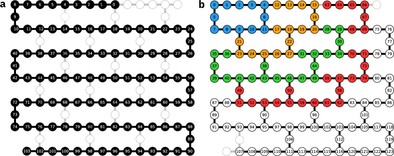
Fig. S7: Mapping virtual to physical qubits in the quantum processor. The figures depict the topology of the 127-qubit quantum processors ibm_washington overlaid with virtual qubit embeddings used in our experiments. Qubits used in the virtual to physical mapping are shaded, colored, and numbered, while the remaining qubits are represented as open rings. a. Schematic of the 104-qubit 1D chain used for studying spin imbalance. b. Schematic of the 124-qubit 2D lattice. The various colors of the qubits illustrate the growth in system size for the OPDM experiments. Specifically, blue indicates the smallest system (1-hexagon), orange indicates the additional qubits for a 3-hexagon system, green represents the increase to a 6-hexagon system, and red denotes the additional qubits used for a 10-hexagon system.

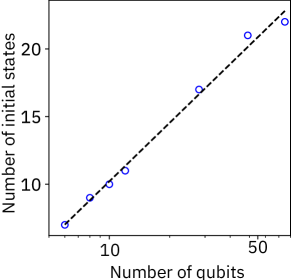
Fig. S8: Circuit sampling complexity for one-particle density (OPDM) reconstruction. The number of initial states shown on a logarithmic scale needed to evaluate all matrix elements of the OPDM as a function of the number of qubits, for a single disorder realization. The relationship exhibits a close match to the logarithmic scaling curve, depicted as a dashed line.

II.1 Quantum circuits

The circuit design for both one and two dimensions involves nearest-neighbor coupling between qubits using a single controlled-Z gate per cycle. This gate is further decomposed into native gates, including a single two-qubit controlled-X gate and Hadamard gates acting on the target qubit on either side of the gate. The error of the controlled-X gate, with a median average $\sim$1.1% on ibm_washington, is typically one or two orders of magnitude larger than that of a single-qubit gate, which has a median error $\sim$0.03%. Therefore, our selected model promotes more efficient use of IBM quantum hardware. In particular, each Floquet step requires only gate depth of two, measured in two-qubit gates, for one dimensional (1D) circuits. In two dimensional circuits (2D), the required gate depth is three. This is in contrast to a generic two-qubit gate which may require a depth up to six (or nine), as in the case of the first-order trotterized Heisenberg model.

The coupling between qubits is mediated by $U(\theta)=U_{3}(\theta,0,\pi)$ gates (as defined by OpenQASM 3.0 convention). The coupling angle $\theta$ ranges from 0 to $\pi$, with $\theta\approx 0.16\pi$ marking the finite-size MBL phase transition. Each $U(\theta)$ gate can be decomposed into two hardware native $SX$ gates and two virtual $RZ$ gates.

After each layer of $CZ$ and $U(\theta$) gates, a phase gate $P(\phi_{i})$ is implemented, representing a disorder $\phi_{i}$ for the qubit $i$. The disorder phases $\phi_{i}$ are randomly drawn from a uniform distribution between $-\pi$ and $\pi$. The total number of two-qubit $CX$ gates can be calculated as $(n-1)D$, where $n$ is the number of qubits and $D$ is the number of Floquet cycles. For example, for the 1D spin imbalance measurement on 104 qubits with $N_{\mathrm{Floquet}}=19$ Floquet cycles, this amounts to 1,957 gates in total.

The 2D circuits are similar to the 1D circuits, except that due to the connectivity of the 2D heavy hexagonal lattice, each Floquet cycle requires 3 layers of $CZ$ and $U(\theta)$ gates, where the layers correspond to the colors of the connections between qubits in Fig. 4a in the main text. The total number of gates is $N_{\mathrm{edges}}\times N_{\mathrm{Floquet}}$, e.g. the quantum circuit for the 2D spin imbalance measurement on 124 qubits with $N_{\mathrm{edges}}=139$ and $N_{\mathrm{Floquet}}=19$ Floquet cycles has 2,641 $CX$ gates.

II.2 Initialization and measurement protocols

Our experimental approach involves measurements aimed at reconstructing three distinct types of objects: spin imbalances, one-particle density matrices (OPDMs), and local integrals of motion (LIOMs). To obtain these, we employ the three-stage procedure on a quantum computer: state initialization, Floquet evolution, and the actual measurement process. In the following, we detail the methods used to measure each of these quantities, providing a comprehensive overview of our approach.

Spin imbalance. Spin imbalance is defined to be

$$\mathcal{I}\coloneqq\frac{n_{1}-n_{0}}{n_{1}+n_{0}}\;,$$ (S.71)

where $n_{0}$ and $n_{1}$ are the average occupation of the sites initialized in the zero and one states, respectively. All spin imbalance measurements were performed on ibm_washington. The initial layout for the 1D chain is shown in Fig. S7a. We initialize the system in a state where each qubit is set to the $|0\rangle$ state. Next, we set certain qubits (see Fig. S4) to the $|1\rangle$ state using an $X$ gate composed of two hardware-native and low-error (typically $\sim 3\cdot 10^{-4}$ as measured by fidelity) $\sqrt{X}$ gates.

For each value of the coupling angle ($\theta=0.1\pi$ and $\theta=0.3\pi$), we independently run 20 circuits with the number of Floquet cycles ranging from 0 to 19. For each cycle, at the end of the evolution, we measure the spin imbalance in Eq. (S.12) based on the expectation values of the qubits in the computational basis. Since qubits can be measured simultaneously, each spin imbalance measurement requires a total of 20 different circuits. Each circuit is run for 8,000 shots to collect the necessary statistics for the expectation.

One-particle density matrix (OPDM). All measurements are performed on ibmq_kolkata (1D) and ibm_washington (2D). We use quantum hardware to obtain the matrix elements of Eq. (S.14), which can be expressed as

$$\begin{split}\rho_{ij}=&\frac{1}{4}\Bigl{(}\langle X_{i}X_{j}\rangle_{c}-i\langle X_{i}Y_{j}\rangle_{c}+i\langle Y_{i}X_{j}\rangle_{c}+\langle Y_{i}Y_{j}\rangle_{c}\Bigl{)},\end{split}$$ (S.72)

where $\langle AB\rangle_{c}=\langle AB\rangle-\langle A\rangle\langle B\rangle$ is the connected correlation function, and $\langle A\rangle:=\langle\psi_{0}|U_{F}^{d{\dagger}}AU^{d}_{F}|\psi_{0}\rangle$ is the expectation of the operator with respect to the time-evolved initial ordered state $|\psi_{0}\rangle$.

For both, the 1D and 2D cases, we start by initializing the system in the geometry-dependent CDW state and then evolve for 10 Floquet cycles. For both cases, we measure qubits in the computational, or $Z$, basis, as well as various combinations of the $X$ and $Y$ bases. The number of combinations should be sufficient to determine all expectations of the operators $\langle X_{i}\rangle$ and $\langle Y_{i}\rangle$, as well as $\langle X_{i}X_{j}\rangle$, $\langle Y_{i}Y_{j}\rangle$, $\langle X_{i}Y_{j}\rangle$, and $\langle Y_{i}X_{j}\rangle$. It is important to note that measuring $O(\log(n))$ random combinations of $X$ and $Y$ bases is sufficient for this purpose [elben2023randomized]. We further develop a simple optimization algorithm that requires a smaller number of multiqubit bases compared to random combinations. The sample complexity of the resulting measurement sequence is illustrated in Fig. S8.

For the one-dimensional circuits, we perform measurements in $\{7,9,10\}$ multi-qubit Pauli basis combinations for system sizes of $\{6,8,10\}$ qubits each, using a single initial state $|10...10\rangle$. The measurements are performed for coupling angles $\theta/\pi=\{0,0.05,0.10,0.15,0.20,0.25\}$ and 100 disorder realizations, resulting in a total of 15,600 circuits. For the 2D OPDMs, we use $\{11,17,21,22\}$ multi-qubit Pauli basis measurements for lattices with $\{1,3,6,10\}$ heavy hexagons (or $\{12,28,49,75\}$ qubits) for the CDW initial state for the same set of coupling angles. The layout is shown in Fig. S7b. The number of disorder realizations for system size containing $n$ qubits is calculated as $\lfloor 625/n\rfloor$, resulting in a total of 8,244 circuits.

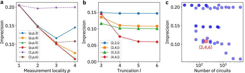
Fig. S9: Cost-benefit analysis for LIOM reconstruction in the presence of noise. This analysis uses a noiseless 10-qubit chain simulation for cycle depth $D=9$ with $L^{(0)}$ chosen as the Pauli $Z$ operator acting on the central qubit $5$ (qubits are numbered starting with 1). The results are averaged over 50 disorder realizations. a. The LIOM imprecision in Eq. (S.19) for various settings as a function of the maximum operator support. Solid lines represent the $(p,p,l)$ setting, dashed lines represent the $(p,k,l)$ setting. Increasing the locality leads to a drastic improvement in imprecision. b. The dependence of the error on the parameter $l$, which sets the number of initial states. c. The trade-off between the method error and the required quantum computational resources for $(p,k,l)$ schemes, where the dots represent different combinations of the settings $1\leq l\leq 4$, $1\leq p\leq 4$, and $1\leq l\leq 6$. The red dot indicates the choice of the experimental setting ($(2,4,6)$).

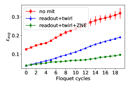
Fig. S10: Benchmarking error mitigation. The average error $\epsilon_{\mathrm{avg}}$ is the root mean square error (RMSE) between the measured and ideal expectation, averaged over all single-qubit $Z_{i}$, for an 8-qubit 1D chain with $\theta=0.1\pi$. We compare unmitigated (“no mit”); mitigated with readout calibration and twirling; and with the addition of zero-noise extrapolation with noise factors for [1, 3] and linear extrapolation. Error bars correspond to the standard error of the RMSE of the single-qubit $Z_{i}$ expectation values.

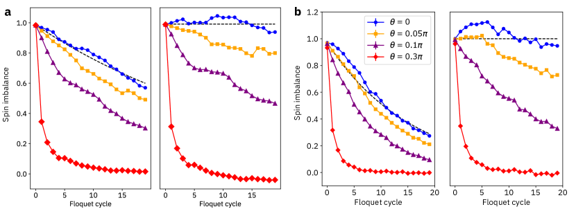
Fig. S11: Dynamics of spin imbalance. Results are shown for coupling angles $\theta/\pi=0$ (blue, circles), $0.05$ (orange, squares), $0.10$ (purple, triangles), and $0.3$ (red, diamonds). The bootstrapped error associated with the shot statistics is smaller that the size of the points. a. The non-normalized (left) and the normalized (right) imbalance for a one-dimensional 104-qubit chain. The non-normalized curves correspond to the error-mitigated results obtained from the device using Eq. (S.71) The normalization is performed by the average slope of the $\theta=0$ curve (dashed curve). b. Similar curves for the 124 qubit hexagonal circuit.

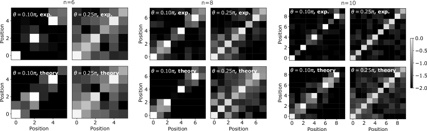
Fig. S12: One-particle density matrices (OPDMs) in 1D lattices. The color plots show the absolute values of the matrix elements $|\rho_{ij}|$ in Eq. (2) for 1D chains with $n=6$, 8, and 10 qubits after $10$ Floquet cycles. The top panels show experimental data, while the bottom panels show theoretical predictions. The color scale is logarithmic, and the black color represents values smaller than $10^{-2}$.

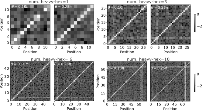
Fig. S13: One-particle density matrices (OPDMs) in 2D lattices.. We consider circuits containing 1, 3, 6, and 10 heavy hexagons for a state after $10$ Floquet cycles. The anomaly at position 66 for the OPDM for the 10 heavy hexagon circuit is due to a high readout error on this qubit. In the gap ratio and discontinuity shown in Figs. 4d and S14 respectively, we remove this entire row and column before calculating the spectrum. The color scale is logarithmic, and the black color represents values smaller than $10^{-3}$.

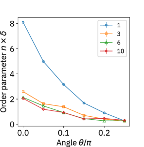
Fig. S14: Discontinuity in the one-particle density matrix (OPDM) in 2D lattices. The plot shows the rescaled discontinuity $n\delta$ multiplied by the number of qubits $n$ for two-dimensional circuits containing 1 (blue), 3 (orange), 6 (green), and 10 (red) hexagons. The parameter saturates to a system-independent value for more than one hexagon (see discussion in the text).

Local integrals of motion. All measurements are performed on ibm_washington (both 1D and 2D). To obtain the value of the correlation function in Eq. (S.33), we measure the quantities

$$f_{\mu d\alpha}=\langle\psi_{\alpha}|U_{F}^{d{\dagger}}P_{\mu}U^{d}_{F}|\psi_{\alpha}\rangle,$$ (S.73)

where $|\psi_{\alpha}\rangle$ denotes the initial states, $P_{\mu}\in Q$ denotes a collection of local Pauli matrices that are part of a predefined set $Q$. Similar to previous experiments, the desired result can be achieved by running multiple runs of a quantum circuit. This process involves initializing the system in the state $|\psi_{\alpha}\rangle$, passing it through $d$ Floquet cycles, and then performing measurements of Pauli operators $P_{\mu}$. A major challenge in this procedure is to determine the optimal set of initial states $|\psi_{\alpha}\rangle$ to reliably estimate the value of $W_{D}(P_{\mu},L^{(0)})$ in Eq. (S.33).

The simplest and scalable method for selecting initial states is to assign them as random bit strings, using the Monte Carlo method. While this method is scalable (requiring $O(1)$ states to estimate the expectation of local operators), it is not an optimal use of resources for shallow circuits. In fact, to achieve an accuracy of $1\%$, we need about $10^{4}$ random initial states. Instead, we use a technique that allows us to achieve comparable accuracy, but with two orders of magnitude fewer initial states.

In one dimension, we choose a family of periodic states $|\psi_{\alpha}\rangle=|w_{\alpha}\rangle\otimes|w_{\alpha}\rangle\otimes\dots\otimes|w_{\alpha}\rangle$, where $|w_{\alpha}\rangle$ represents possible combinations of $l$ bit strings. The number of such states is only $2^{l}$. At the same time, for any evolution $U^{d}_{F}$ that transforms a local operator into an operator with support on $l$ qubits or less, expectation over this set of initial states is as effective as over all $2^{n}$ states.

For the two-dimensional heavy hexagonal lattice configuration, we find a similar suitable set of states. We first represent the Floquet cycle as a graph with vertices representing the qubits and the edges corresponding to next-neighbor connections. Next, we construct a randomized search algorithm that colors the graph using $l$ unique colors such that it minimizes the number of colors within $r$ steps of each qubit. The result is equivalent to the initial set of $2^{l}$ states, where each uniquely colored qubit represents an independently chosen value 0 or 1. As in the 1D case, the precision can be improved by choosing larger $l$.

Next, we develop a measurement protocol to get the values of the Pauli operators $P_{\mu}$. In one dimension, we choose to measure qubits at positions $i$, $i+p$, $i+2p$, and so on, in the same basis chosen from $X$, $Y$, or $Z$ for some integer $p\geq 1$. This pattern results in $3^{p}$ measurement combinations, which allows us to measure all local $4^{p}-1$ Pauli operators $P_{\mu}$ with support $p$. In addition, the protocol allows to measure some of the Pauli operators with support $k>p$. We then measure all such Pauli operators and include them in the set $Q$.

To choose the Pauli measurement in two dimensions, we return to the graph representation of the Floquet cycle. We then use an algorithm that solves a graph coloring problem using $p$ colors so that each path containing $k$ qubits contains as many different colors as possible. Each such color corresponds to an independently chosen qubit measurement basis. This allows to measure all $k$-local Pauli operators if $p=k$, and fraction of them otherwise. For $p=2$, the best choice is the antiferromagnetic coloring shown in Fig. (S4)b.

Combining the initialization protocol and the measurement protocol, we obtain a method we call the $(p,k,l)$ scheme. For this scheme, we use $2^{l}$ initial state combinations and $3^{p}$ Pauli measurement combinations to obtain all possible expectations of Pauli operators with support up to $k$. For any such scheme, the total number of unique quantum circuits required to run is $N_{\rm circ}=D\times 2^{l}\times 3^{p}$, where the factor of $D$ comes from the fact that we need to perform the measurements for each depth instance $d\in\{0,\dots,D-1\}$.

The analysis of different schemes in 1D, including their effect on the imprecision and the number of circuits required, is shown in Fig. S9. For example, Fig. S9a and Fig. S9b show how the LIOM imprecision is reduced by increasing $p$ and $l$. While this reduction can be significant, the number of circuits grows exponentially with these parameters. To make the best choice, we perform the cost-benefit analysis shown in Fig. S9c. We found that the best scheme to achieve high precision with a reasonable number of circuits that exhibits sufficiently wide LIOMs is the $(2,4,6)$ scheme (marked by the red dot). In our experiment shown in Figs. 3 and 4 we use this scheme including $N_{\rm circ}=10\times 64\times 9=5,760$ of non-mitigated circuits in total. This allows us to evaluate all values in Eq. (S.73) for all two-qubit Pauli operators and some three- and four-qubit Pauli operators. We use the same scheme and parameters for the two-dimensional setting, although we are unable to estimate the precision classically.

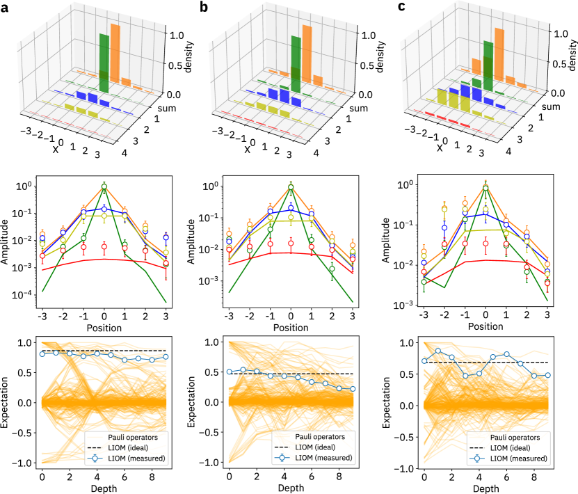
Fig. S15: Examples of local integrals of motion (LIOMs) with varying levels of error. The plot illustrates three LIOMs with different levels of imprecision: the lowest error (panel a, $\epsilon=0.065$), the median error (panel b, $\epsilon=0.135$), and the highest error (panel c, $\epsilon=0.357$). The top subpanels display the density of the LIOMs, while the middle subpanels present a logarithmic scale plot comparing the LIOM to the theoretical curve derived from the limited-size numerical simulation. The bottom subpanels depict the time dependence of the involved Pauli operators (orange curves) and the expectation value of the LIOM itself. The dashed line represents the ideal behavior of the LIOM for infinite-depth evolution, as derived from the limited-size numerical simulation. All numerics use 12-qubit sub-regions to approximate the behavior of the LIOMs in the larger 104-qubit system.

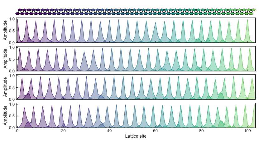
Fig. S16: Operator density representation for 104 LIOMs in a 1D spin chain. This graph provides an experimental reconstruction of operator amplitudes for each of the 104 Local Integrals of Motion (LIOMs) in a 104-qubit chain, depicted schematically above the topmost plot. For improved readability and to prevent overlap, the LIOMs are distributed across four axes to enhance visual spacing. More specifically, the topmost axis displays the LIOMs at sites $i=0,4,8,\ldots$, the second from the top axis shows the LIOMs at sites $i=1,5,9,\ldots$, and so forth. The y-axes represent the operator spatial amplitudes $W(x)=\sqrt{\sum_{\mu}a_{\mu}^{2}w_{x\mu}}$, where $a_{\mu}$ is the reconstructed coefficients for the Pauli $\mu$ operator in a LIOM decomposition and $w_{x\mu}$ is the weight associated this Pauli operator at site $x$.

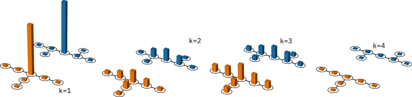
Fig. S17: Structure of local integrals of motion (LIOMs) in a 2D lattice. The figure illustrates the decomposition of the “average” LIOM into contributions from $k$-local Pauli operators, for $k$ in the range from 1 to 4. The blue bars represent the two-vertex configuration, while the orange bars represent the three-vertex configuration.

II.3 Error mitigation

Quantum error mitigation [Cai2022] describes strategies aimed at mitigating the detrimental effects of noise in quantum computations. Two popular and primary strategies are zero-noise extrapolation (ZNE) [Li2017ZNE, Temme2017PECandZNE] and probabilistic error cancellation (PEC) [Temme2017PECandZNE, Berg2022, Berg2022TREX], which have recently been combined in [Kim2023].

Here, we developed a tailored, composite error-suppression and mitigation strategy that includes logical-to-physical qubit mapping [Nation2023Mapomatic], M3 readout mitigation [Nation2021M3], Pauli twirling [Wallman2017Twirling], and ZNE [Li2017ZNE, Temme2017PECandZNE, GiurgicaTiron2020ZNEReviewAndAdaptive]. This strategy is straightforwardly scalable to large system sizes and accessible via open-sourced packages offered through the Qiskit ecosystem.

First, virtual qubits in the quantum circuit are mapped to physical qubits on the device. In the case of the 104-qubit 1D chain, the 124-qubit 2D lattice, and the 2D OPDM measurements, there are limited possibilities for this mapping. For the 1D OPDMs measured on 6, 8, or 10 qubits, the best qubits for a given circuit on a given device are selected using the Qiskit package mapomatic [Nation2023Mapomatic]. Based on the connectivity of the transpiled circuit, mapomatic finds possible mappings between virtual and physical qubits of a given device, ranks them based on a simple cost function that takes into account the characterized errors of each qubit and gate, and selects the best one.

In order to mitigate coherent errors during runtime, we employ a combination of two strategies. The first strategy involves applying a technique known as “twirling” to the noise present in the two-qubit gate layers of the circuits [Wallman2017Twirling]. For a tutorial on twirling, see Ref. [Minev2022twirl]. This approach entails the addition of random single-Pauli gates before and after the noisy two-qubit gates. These gates serve to “mix up” the noise, helping to reduce its impact. Notably, the errors associated with the two-qubit gates are typically an order of magnitude larger than those of the single-qubit gates. We randomly sample the twirled circuits $N_{\mathrm{twirl}}=5$ times and run each twirled circuit with $1/N_{\mathrm{twirl}}$ of the shots for the original circuit. The second strategy is dynamical decoupling (DD), which can suppress crosstalk errors [Viola1999DD, Jurcevic2021]. Here, we insert evenly spaced XY4 pulses in idle periods for 1D single particle density matrix measurements, but do not use DD for spin imbalance and local integrals of motion measurements on larger systems as the brickwork quantum circuits have little idle time.

We also mitigate readout and incoherent errors by running additional circuits. Readout errors are mitigated on the noisy bitstring-level with the quasi-probability-based M3 method [Nation2021M3]. The “balanced” version of the method requires $2N_{\mathrm{qubit}}$ readout calibration circuits to be run as opposed to the full matrix-inversion method that requires $2^{N_{\mathrm{qubit}}}$ calibration circuits [Bravyi2021ReadoutMatrixInversion], which is infeasible for the system sizes considered here. We empirically find that the readout calibration need only be repeated every hour or so to maintain the performance of readout mitigation. Because many of the circuits—over many Floquet cycles, measurement bases, and initial states—in this study are run on the same qubits, running the readout calibration circuits incurs only a small overhead. Incoherent errors are mitigated with digital zero-noise extrapolation (ZNE) [Li2017ZNE, Temme2017PECandZNE, GiurgicaTiron2020ZNEReviewAndAdaptive]. In dZNE, additional digital quantum gates that resolve to identity are inserted into the circuit to amplify the noise. Expectation values are computed at multiple noise factors, where a noise factor of 1 corresponds to the original circuit and, e.g., a noise factor of 3 corresponds to appending the inverse of the circuit followed by the circuit itself. Then, the zero-noise expectation value is estimated by extrapolating from the expectation values at these non-zero noise factors. In this study, we use noise factors of 1 and 3, and we use linear extrapolation, which generally underestimates the magnitude of observables but is more stable than exponential extrapolation.

We quantify the improvement in noisy expectation values in Fig. S10 with and without quantum error mitigation for an 8-qubit Floquet circuit with $\theta=0.1\pi$ and find that, after 20 Floquet cycles, the average single-qubit $Z_{i}$ error is around 0.1 using the best settings for zero-noise extrapolation.

Finally, error due to shot noise propagated through the error mitigation pipeline and data post-processing is quantified via bootstrapping over the bitstring counts.

Overall, this composite error mitigation strategy involves minimal additional classical compute to twirl the circuits and insert DD pulses, as well as minimal overhead of quantum resources—the total shot count of the entire composite strategy is just twice that of the unmitigated execution due to ZNE.

III Additional data

In this section, we present additional experimental data to support the claims of the paper. Below, we simply list the additional results and provide the accompanying description.

Additional data on spin imbalance. Figure S11 extends the plots presented in Figs. 2c and 4c by showing non-normalized imbalance values and the dynamics of the circuits for both $\theta=0$ and $\theta=0.05\pi$. The plots show a significant decay of the imbalance at $\theta=0$, even though the circuit must exhibit no dynamics if applied to a state in the computational basis. This decay can be attributed to the presence of noise. To mitigate the effect of noise, we perform a partial compensation by renormalizing the remaining curves using the average decay curve of $\theta=0$, which is represented by the dashed black curve. The result of this normalization process can be observed in the right subpanels and is also shown in the main text. In Fig. 2c, we have performed a fit analysis of the MBL regime data using the fit function $\mathcal{I}(d)=\mathcal{I}_{s}+(1-\mathcal{I}_{s})\exp(-\gamma d)$, where we find $\mathcal{I}_{s}=0.425$ and $\gamma=0.0966$ (blue dashed curve). The horizontal dotted line in the figure visually represents the value of $\mathcal{I}_{0}$.

Additional data on OPDMs. Figure S12 provides a visual representation of the OPDM for one-dimensional chains composed of 6, 8, and 10 qubits. This state has evolved over $D=10$ cycles for a specific disorder realization. In addition to the experimental data, the figure also shows theoretical predictions. In the ergodic regime ($\theta=0.3\pi$), the off-diagonal elements become more prominent, while the diagonal elements show a more uniform pattern compared to the MBL regime ($\theta=0.1\pi$). The average spectra resulting from the diagonalized OPDMs are shown in the main text in Fig. 2c.

Figure S13 shows similar data for the OPDMs of 2D lattices containing 1, 3, 6, and 10 heavy hexagons. These correspond to 12, 28, 49, and 75 qubits, respectively. The corresponding circuit layouts for these configurations are shown in Fig. S7b. As with the one-dimensional system, we consider a state that has evolved over $D=10$ Floquet cycles for a singular disorder realization. The gap contrast of the spectra from the diagonalized OPDMs is shown in the main text in Fig. 4d.

Figure S14 shows the rescaled discontinuity, similar to that shown in Fig. 2d for the one-dimensional circuit. However, unlike the one-dimensional system, this parameter does not exhibit a system-size scaling that depends on the coupling angle $\theta$ values for more than a single heavy hexagon. This phenomenon can be attributed to the strong influence of noise, which technically closes the hard gap in the OPDM spectrum for small $\theta$, resulting in a “soft” gap (i.e. region of significantly reduced density without a real gap). As a result, the $n\delta$ parameter plateaus at a constant value that is independent of the system size. The thermalization process of the system as a function of system size can still be examined by observing the gap ratio in Fig. 4d, which is applicable to both hard and soft gaps.

Additional data on LIOMs. Figure S15 presents additional examples of individual approximate LIOMs for comparison. Here one can compare individual LIOMs with the ‘average’ approximate LIOM shown in Figure 3b in the main text. For demonstration purposes, we have chosen three LIOMs with different levels of imprecision: the smallest, the median, and the highest. It is noteworthy that these operators have very similar shapes. We also plot the time dependence of each approximate LIOM as a function of cycle depth. As expected, the LIOM with the highest imprecision shows noticeable oscillations.

In Fig. S16, we present a depiction of all 104 Local Integrals of Motion (LIOMs), as experimentally reconstructed in the one-dimensional, 104-qubit experiment. Each LIOM is localized around a specific qubit site, exhibiting a distinct spatial extent and profile influenced by both the interactions and disorder realization. The amplitude of the weight assigned to each LIOM is plotted to showcase the varying spatial contributions across the entirety of weight Paulis. Due to the substantial overlap among the LIOMs, we have opted to distribute them across four axes for clearer visualization.

In Fig. S17, we decompose the LIOM density shown in Fig. 4e into contributions from one-local to four-local Pauli operators. Similar to the one-dimensional scenario, the dominant contribution comes from the one-local Pauli operators, with a single Pauli $Z$ acting on the central qubit having the largest contribution. Interestingly, the three-local contribution is nearly equal to the two-qubit contributions, suggesting quantum scrambling dynamics in the system.

References

- Arnol’d [2013] V. I. Arnol’d, Mathematical methods of classical mechanics, Vol. 60 (Springer Science & Business Media, 2013).
- Caux and Mossel [2011] J.-S. Caux and J. Mossel, Remarks on the notion of quantum integrability, J. Stat. Mech.-Theory E. 2011, P02023 (2011).
- Sutherland [2004] B. Sutherland, Beautiful Models: 70 Years of Exactly Solved Quantum Many-body Problems (World Scientific, 2004).
- Shiraishi and Matsumoto [2021] N. Shiraishi and K. Matsumoto, Undecidability in quantum thermalization, Nature communications 12, 5084 (2021).
- Basko et al. [2006] D. M. Basko, I. L. Aleiner, and B. L. Altshuler, Metal–insulator transition in a weakly interacting many-electron system with localized single-particle states, Ann. Phys. 321, 1126 (2006).
- Pal and Huse [2010] A. Pal and D. A. Huse, Many-body localization phase transition, Phys. Rev. B 82, 174411 (2010).
- Nandkishore and Huse [2015] R. Nandkishore and D. A. Huse, Many-body localization and thermalization in quantum statistical mechanics, Annu. Rev. Condens. Matter Phys. 6, 15 (2015).
- Abanin et al. [2019] D. A. Abanin, E. Altman, I. Bloch, and M. Serbyn, Colloquium: Many-body localization, thermalization, and entanglement, Rev. Mod. Phys. 91, 021001 (2019).
- Serbyn et al. [2013] M. Serbyn, Z. Papić, and D. A. Abanin, Local conservation laws and the structure of the many-body localized states, Phys. Rev. Lett. 111, 127201 (2013).
- Huse et al. [2014] D. A. Huse, R. Nandkishore, and V. Oganesyan, Phenomenology of fully many-body-localized systems, Phys. Rev. B 90, 174202 (2014).
- De Roeck and Huveneers [2017] W. De Roeck and F. m. c. Huveneers, Stability and instability towards delocalization in many-body localization systems, Phys. Rev. B 95, 155129 (2017).
- Morningstar et al. [2022] A. Morningstar, L. Colmenarez, V. Khemani, D. J. Luitz, and D. A. Huse, Avalanches and many-body resonances in many-body localized systems, Phys. Rev. B 105, 174205 (2022).
- Sels [2022] D. Sels, Bath-induced delocalization in interacting disordered spin chains, Phys. Rev. B 106, L020202 (2022).
- Léonard et al. [2023] J. Léonard, S. Kim, M. Rispoli, A. Lukin, R. Schittko, J. Kwan, E. Demler, D. Sels, and M. Greiner, Probing the onset of quantum avalanches in a many-body localized system, Nat. Phys. 19, 481 (2023).
- Rispoli et al. [2019] M. Rispoli, A. Lukin, R. Schittko, S. Kim, M. E. Tai, J. Léonard, and M. Greiner, Quantum critical behaviour at the many-body localization transition, Nature 573, 385 (2019).
- Lukin et al. [2019] A. Lukin, M. Rispoli, R. Schittko, M. E. Tai, A. M. Kaufman, S. Choi, V. Khemani, J. Léonard, and M. Greiner, Probing entanglement in a many-body–localized system, Science 364, 256 (2019).
- Roushan et al. [2017] P. Roushan, C. Neill, J. Tangpanitanon, V. M. Bastidas, A. Megrant, R. Barends, Y. Chen, Z. Chen, B. Chiaro, A. Dunsworth, et al., Spectroscopic signatures of localization with interacting photons in superconducting qubits, Science 358, 1175 (2017).
- Choi et al. [2016] J.-y. Choi, S. Hild, J. Zeiher, P. Schauß, A. Rubio-Abadal, T. Yefsah, V. Khemani, D. A. Huse, I. Bloch, and C. Gross, Exploring the many-body localization transition in two dimensions, Science 352, 1547 (2016).
- Schreiber et al. [2015] M. Schreiber, S. S. Hodgman, P. Bordia, H. P. Lüschen, M. H. Fischer, R. Vosk, E. Altman, U. Schneider, and I. Bloch, Observation of many-body localization of interacting fermions in a quasirandom optical lattice, Science 349, 842 (2015).
- Smith et al. [2016] J. Smith, A. Lee, P. Richerme, B. Neyenhuis, P. W. Hess, P. Hauke, M. Heyl, D. A. Huse, and C. Monroe, Many-body localization in a quantum simulator with programmable random disorder, Nat. Phys. 12, 907 (2016).
- Bordia et al. [2017a] P. Bordia, H. Lüschen, U. Schneider, M. Knap, and I. Bloch, Periodically driving a many-body localized quantum system, Nat. Phys. 13, 460 (2017a).
- Bordia et al. [2017b] P. Bordia, H. Lüschen, S. Scherg, S. Gopalakrishnan, M. Knap, U. Schneider, and I. Bloch, Probing slow relaxation and many-body localization in two-dimensional quasiperiodic systems, Phys. Rev. X 7, 041047 (2017b).
- Guo et al. [2021] Q. Guo, C. Cheng, Z.-H. Sun, Z. Song, H. Li, Z. Wang, W. Ren, H. Dong, D. Zheng, Y.-R. Zhang, R. Mondaini, H. Fan, and H. Wang, Observation of energy-resolved many-body localization, Nat. Phys. 17, 234 (2021).
- Mi et al. [2022] X. Mi, M. Ippoliti, C. Quintana, A. Greene, Z. Chen, J. Gross, F. Arute, K. Arya, J. Atalaya, R. Babbush, et al., Time-crystalline eigenstate order on a quantum processor, Nature 601, 531 (2022).
- Sels and Polkovnikov [2023] D. Sels and A. Polkovnikov, Thermalization of dilute impurities in one-dimensional spin chains, Phys. Rev. X 13, 011041 (2023).
- [26] See Supplementary Materials.
- Zhang et al. [2016] L. Zhang, V. Khemani, and D. A. Huse, A floquet model for the many-body localization transition, Phys. Rev. B 94, 224202 (2016).
- Ponte et al. [2015] P. Ponte, Z. Papić, F. m. c. Huveneers, and D. A. Abanin, Many-body localization in periodically driven systems, Phys. Rev. Lett. 114, 140401 (2015).
- Nahum et al. [2018] A. Nahum, S. Vijay, and J. Haah, Operator spreading in random unitary circuits, Phys. Rev. X 8, 021014 (2018).
- Bera et al. [2015] S. Bera, H. Schomerus, F. Heidrich-Meisner, and J. H. Bardarson, Many-body localization characterized from a one-particle perspective, Phys. Rev. Lett. 115, 046603 (2015).
- Bera et al. [2017] S. Bera, T. Martynec, H. Schomerus, F. Heidrich-Meisner, and J. H. Bardarson, One-particle density matrix characterization of many-body localization, Ann. Phys. (Berlin) 529, 1600356 (2017).
- Elben et al. [2023] A. Elben, S. T. Flammia, H.-Y. Huang, R. Kueng, J. Preskill, B. Vermersch, and P. Zoller, The randomized measurement toolbox, Nat. Rev. Phys. 5, 9 (2023).
- Mahan [2000] G. D. Mahan, Many-particle physics (Springer Science & Business Media, 2000).
- Mierzejewski et al. [2015] M. Mierzejewski, P. Prelovšek, and T. c. v. Prosen, Identifying local and quasilocal conserved quantities in integrable systems, Phys. Rev. Lett. 114, 140601 (2015).
- Chandran et al. [2015] A. Chandran, I. H. Kim, G. Vidal, and D. A. Abanin, Constructing local integrals of motion in the many-body localized phase, Phys. Rev. B 91, 085425 (2015).
- Kim et al. [2023a] Y. Kim, A. Eddins, S. Anand, K. X. Wei, E. van den Berg, S. Rosenblatt, H. Nayfeh, Y. Wu, M. Zaletel, K. Temme, and A. Kandala, Evidence for the utility of quantum computing before fault tolerance, Nature 618, 500 (2023a).
- Burrell and Osborne [2007] C. K. Burrell and T. J. Osborne, Bounds on the speed of information propagation in disordered quantum spin chains, Phys. Rev. Lett. 99, 167201 (2007).
- Kim et al. [2023b] Y. Kim, C. J. Wood, T. J. Yoder, S. T. Merkel, J. M. Gambetta, K. Temme, and A. Kandala, Scalable error mitigation for noisy quantum circuits produces competitive expectation values, Nat. Phys. 10.1038/s41567-022-01914-3 (2023b).
- Cai et al. [2022] Z. Cai, R. Babbush, S. C. Benjamin, S. Endo, W. J. Huggins, Y. Li, J. R. McClean, and T. E. O’Brien, Quantum error mitigation, arxiv:2210.00921 (2022).
- Li and Benjamin [2017] Y. Li and S. C. Benjamin, Efficient variational quantum simulator incorporating active error minimization, Phys. Rev. X 7, 021050 (2017).
- Temme et al. [2017] K. Temme, S. Bravyi, and J. M. Gambetta, Error mitigation for short-depth quantum circuits, Phys. Rev. Lett. 119, 180509 (2017).
- van den Berg et al. [2023] E. van den Berg, Z. K. Minev, A. Kandala, and K. Temme, Probabilistic error cancellation with sparse pauli–lindblad models on noisy quantum processors, Nature Physics 10.1038/s41567-023-02042-2 (2023).
- van den Berg et al. [2022] E. van den Berg, Z. K. Minev, and K. Temme, Model-free readout-error mitigation for quantum expectation values, Phys. Rev. A 105, 032620 (2022).
- Nation and Treinish [2023] P. D. Nation and M. Treinish, Suppressing quantum circuit errors due to system variability, PRX Quantum 4, 010327 (2023).
- Nation et al. [2021] P. D. Nation, H. Kang, N. Sundaresan, and J. M. Gambetta, Scalable mitigation of measurement errors on quantum computers, PRX Quantum 2, 040326 (2021).
- Wallman and Emerson [2016] J. J. Wallman and J. Emerson, Noise tailoring for scalable quantum computation via randomized compiling, Phys. Rev. A 94, 052325 (2016).
- Giurgica-Tiron et al. [2020] T. Giurgica-Tiron, Y. Hindy, R. LaRose, A. Mari, and W. J. Zeng, Digital zero noise extrapolation for quantum error mitigation, in 2020 IEEE International Conference on Quantum Computing and Engineering (QCE) (2020) pp. 306–316.
- Minev [2022] Z. Minev, A tutorial on tailoring quantum noise - Twirling 101 (2022).
- Viola et al. [1999] L. Viola, E. Knill, and S. Lloyd, Dynamical decoupling of open quantum systems, Phys. Rev. Lett. 82, 2417 (1999).
- Jurcevic et al. [2021] P. Jurcevic, A. Javadi-Abhari, L. S. Bishop, I. Lauer, D. F. Bogorin, M. Brink, L. Capelluto, O. Günlük, T. Itoko, N. Kanazawa, A. Kandala, G. A. Keefe, K. Krsulich, W. Landers, E. P. Lewandowski, D. T. McClure, G. Nannicini, A. Narasgond, H. M. Nayfeh, E. Pritchett, M. B. Rothwell, S. Srinivasan, N. Sundaresan, C. Wang, K. X. Wei, C. J. Wood, J.-B. Yau, E. J. Zhang, O. E. Dial, J. M. Chow, and J. M. Gambetta, Demonstration of quantum volume 64 on a superconducting quantum computing system, Quantum Sci. Technol. 6, 025020 (2021).
- Bravyi et al. [2021] S. Bravyi, S. Sheldon, A. Kandala, D. C. Mckay, and J. M. Gambetta, Mitigating measurement errors in multiqubit experiments, Phys. Rev. A 103, 042605 (2021).
Supplementary Materials for