Prescaling relaxation to nonthermal attractors

Abstract

We study how isotropic and homogeneous far-from-equilibrium quantum systems relax to nonthermal attractors, which are of interest for cold atoms and nuclear collisions. We demonstrate that a first-order ordinary differential equation governs the self-similar approach to nonthermal attractors, i.e., the prescaling. We also show that certain natural scaling-breaking terms induce logarithmically slow corrections that prevent the scaling exponents from reaching the constant values during the system’s lifetime. We propose that, analogously to hydrodynamic attractors, the appropriate mathematical structure to describe such dynamics is the transseries. We verify our analytic predictions with state-of-the-art $2$PI simulations of the large-$N$ vector model and QCD kinetic theory.

Introduction.– Thermalization of isolated quantum many-body systems is an important contemporary research problem of a broad scope. Its relevance ranges from cold atom systems, through QCD in ultrarelativistic nuclear collisions all the way to gravity and black hole physics [1]. Given the complexity of modeling quantum many-body dynamics and the richness of non-equilibrium phenomena, emergent regularities that form a basis for a quantitative understanding are of particular interest.

In this work we are concerned with an important instance of such an emergent regularity: far-from-equilibrium self-similar time evolution of nonthermal attractors, also known as nonthermal fixed points. These phenomena are transient stages in the thermalization dynamics, whose defining feature is self-similar scaling behavior in time. Consider a momentum distribution function $f(t,\mathbf{p})$ of a homogeneous and isotropic system, where $t$ is time and $\mathbf{p}$ spatial momentum. The system reaches a nonthermal attractor, when $f$ scales with time

$$f(t,\mathbf{p})=(t/t_{\mathrm{ref}})^{\alpha_{\infty}}f_{S}((t/t_{\mathrm{ref}})^{\beta_{\infty}}|\mathbf{p}|)$$ (1)

with constant scaling exponents $\alpha_{\infty}$ and $\beta_{\infty}$. Indeed, such behavior corresponds to a vast reduction in the complexity, as the knowledge of the distribution function at some time allows one to determine the distribution function at a different time by a simple rescaling.

Nonthermal attractors appear in the studies of isolated quantum systems across a wide range of energy scales: ultracold quantum gases [2, 3, 4, 5, 6, 7, 8, 9, 10, 11], ultrarelativistic nuclear collisions [12, 13, 14] and early universe cosmology [15, 16]. Despite significant interest in nonthermal attractors, a quantitative understanding of how a system approaches a nonthermal fixed point remains elusive [17, 18, 19, 20, 21].

In [17] it was proposed that even prior to reaching the nonthermal attractor (1) the system can exhibit prescaling with time dependent scaling exponents $\alpha(t)$ and $\beta(t)$

$$f(t,\mathbf{p})=A(t)\,f_{S}(B(t)|\mathbf{p}|),$$ (2)

where the prescaling factor $A(t)=\exp[\int_{t_{0}}^{t}dt^{\prime}\alpha(t^{\prime})/t^{\prime}]$ reduces to the fixed-point scaling of Eq. (1) when $\alpha(t)$ approaches $\alpha_{\infty}$. The same holds for $B(t)$ in terms of $\beta(t)$.

Given that scaling (1) is an asymptotic late times statement known to be reached slowly, the systems of interest might in fact spend a much greater fraction of their lifetime prescaling (2) rather than scaling (1). Therefore, a quantitative understanding of prescaling is as important as understanding scaling itself.

In our work, we develop a simple theoretical description of prescaling dynamics that uses the same assumptions as the ones used to derive scaling. We test our predictions using strongly-correlated large-$N$ vector model and weak coupling QCD kinetic theory simulations.

Scaling implies prescaling.– Understanding prescaling requires identifying laws governing time evolution of $A(t)$ and $B(t)$ (or, alternatively, $\alpha(t)$ and $\beta(t)$). As we show, these laws have a surprisingly simple origin and form.

The key role in deriving scaling (1) is played by conserved quantities: particle number density $n=\int d^{d}\mathbf{p}\,f/(2\pi)^{d}$ or energy density $\mathcal{E}=\int d^{d}\mathbf{p}\,\omega_{\mathbf{p}}f/(2\pi)^{d}$, where $d$ is the number of spatial dimensions and $\omega_{\mathbf{p}}$ is the dispersion relation of particles. We focus on $\omega_{\mathbf{p}}\sim|\mathbf{p}|^{z}$. Requiring conservation of $n$ or $\mathcal{E}$ is known to impose the relation between the scaling exponents: $\alpha_{\infty}=\sigma\,\beta_{\infty}$ [22]. When $n=\text{const}$, then $\sigma=d$, while $\mathcal{E}=\text{const}$ gives $\sigma=(d+z)$. The conserved quantities are local in time, which means that they in fact constrain also prescaling exponents in exactly the same way: $\alpha(t)=\sigma\,\beta(t)$. Equivalently, $A(t)=B(t)^{\sigma}$. This implies that there is only one independent degree of freedom in the isotropic and homogeneous prescaling, which we will choose to be $B(t)$.

The time evolution for the independent prescaling factor $B(t)$ is still subject to the equation of motion for $f$. In the case of a kinetic theory it is given by the Boltzmann equation with collision kernel ${\cal C}[f]$

$$\partial_{t}f(t,\mathbf{p})={\cal C}[f](t,\mathbf{p}).$$ (3)

In the present section, we assume the collision kernel to be a homogeneous functional of particles momenta, i.e., to simply scale under Eq. (2) by $A(t)^{\mu_{\alpha}}B(t)^{\mu_{\beta}}\equiv B(t)^{\sigma\mu_{\alpha}+\mu_{\beta}}$ for some real numbers $\mu_{\alpha,\beta}$. This assumption applies to many (but not all) collision kernels describing nonthermal attractors. Typically overoccupation singles out terms with the highest power of the distribution function and associated matrix elements often happen to scale homogeneously under rescalings of momenta. For such collision kernels we can separate time-dependent and (rescaled) momentum-dependent contributions in the Boltzmann equation

$$\frac{B(t)^{1-1/\beta_{\infty}}}{\partial_{t}B(t)}=\frac{1}{D_{1}}=\frac{\left[\sigma+\bar{\mathbf{p}}\cdot\partial_{\bar{\mathbf{p}}}\right]f_{S}(\bar{\mathbf{p}})}{{\cal C}[f_{S}](\bar{\mathbf{p}})},$$ (4)

with $\bar{\mathbf{p}}=B(t)\,\mathbf{p}$ being the rescaled momentum, $1/\beta_{\infty}=(1-\mu_{\alpha})\sigma-\mu_{\beta}$, and $D_{1}$ being a separation of variables constant. The intrinsic time dependence of our setup implies nonzero $D_{1}$. The right-hand side of Eq. (4) has the same form for constant scaling exponents but the left-hand side is more general, and is an exact equation of motion for prescaling.

The idea of separation of variables in the context of nonthermal attractors appeared already in [23], but only solutions with constant scaling exponents were considered. In particular, the late time form (1) fixes $D_{1}=\beta_{\infty}/t_{\mathrm{ref}}$. Our key observation here is that prescaling is encapsulated by the general solution of Eq. (4),

$$B(t) =\left(\tfrac{t-t_{*}}{t_{\mathrm{ref}}}\right)^{\beta_{\infty}}\approx\left(\tfrac{t}{t_{\mathrm{ref}}}\right)^{\beta_{\infty}}\left(1-\beta_{\infty}\tfrac{t_{*}}{t}+\ldots\right)$$ (5a)

$$\beta(t) =\beta_{\infty}\tfrac{t}{t-t_{*}}\approx\beta_{\infty}+\beta_{\infty}\tfrac{t_{*}}{t}+\ldots\quad.$$ (5b)

From Eq. (5) it is clear that prescaling induces power-law corrections to scaling. The prescaling originates from the presence of nonzero $t_{*}$. Its appearance comes as no surprise: the dynamics of the system in question is time translationally invariant and therefore $t$ appearing in formulas needs to be measured with respect to some time, $t_{*}$. The reason why it does not appear in Eq. (1) is because the exact scaling is an asymptotic late time statement and dependence on $t_{*}$ drops. Note that while $\beta_{\infty}$ and $\alpha_{\infty}$ are theory specific and independent of initial conditions, $t_{*}$ is going to depend on a chosen initial state.

Before we move to testing Eq. (5) using ab initio solutions of quantum dynamics, let us reiterate that this result originates from the Boltzmann equation and pertinent conservation laws. These are exactly the same constraints as used in a conventional scaling analysis [22]. Prescaling in the case of collision kernels being homogeneous functionals of momenta can therefore be understood as a direct consequence of the existence of scaling.

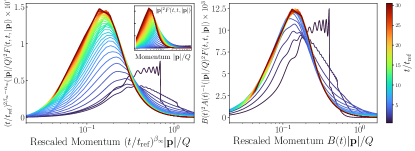
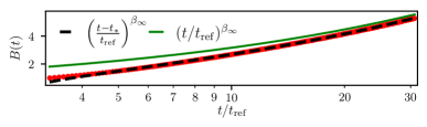
Figure 1: (Top) Statistical function $|\mathbf{p}|^{2}F(t,t,|\mathbf{p}|)$ from 2PI simulations of large-$N$ vector model rescaled with (left) fixed point exponents $(\alpha_{\infty},\beta_{\infty})=(3/2,1/2)$ and (right) with prescaling factors $A(t),B(t)$, where $t_{\mathrm{ref}}\,Q\sim 93$. The unrescaled distribution is shown in the inset. (Bottom) Extracted $B(t)$ compared with Eq. (5a) and asymptotic form.

Prescaling in large-$N$ vector model.– We begin by benchmarking Eq. (5a) against the full quantum dynamics of a large-$N$ vector model at small coupling $\lambda$. The resulting nonthermal fixed point, residing in the infrared, is characterized by $(\alpha_{\infty},\beta_{\infty})=(d/2,1/2$) and was also realized in cold quantum gases [2]. This fixed point arises for large occupations $f\sim 1/\lambda\gg 1$ such that its description requires going beyond a standard kinetic theory analysis. Large-$N$ kinetic theory addresses this regime due to inclusion of relevant resummations [22, 24]. The corresponding collision kernel scales homogeneously with $\mu_{\alpha}=1$ and $\mu_{\beta}=-2$, with the associated scattering matrix element void of scaling breaking terms.

We perform ab initio studies of this fixed point using the $2$PI formalism following [21]. Below the mass gap the equal-time statistical function $F(t,t,|\mathbf{p}|)$ reduces to $f(t,|\mathbf{p}|)$ [22]. Following [17] we extract the prescaling factors $A(t)$ and $B(t)$ from the time evolution of integral moments of $F(t,t,|\mathbf{p}|)$, e.g., $B(t)=n(t)\mathcal{E}(t_{0})/(\mathcal{E}(t)n(t_{0}))$ (see Eq. (A4) in the Appendix). In the upper right panel of Fig. 1 we show how rescaling with $A(t)$ and $B(t)$ leads to an early collapse of distributions at different times, while a considerable spread remains when rescaling with the fixed point exponents (left panel). The evolution of the extracted $B(t)$ is shown in the lower panel to be well described by Eq. (5a) already at early times (dashed black line), and only asymptotes to the corresponding fixed point scaling behavior (1) (solid green line).

Prescaling in isotropic QCD kinetic theory.– We move now to studying prescaling dynamics in QCD, whose nonthermal fixed point plays an important role in our understanding of thermalization dynamics in weakly-coupled models of ultrarelativistic nuclear collisions [1]. We use QCD kinetic theory, where the evolution of the color and polarization averaged gluon distribution function $f(t,\mathbf{p})$ is described by $2\leftrightarrow 2$ and $1\leftrightarrow 2$ processes [25]: $\partial_{t}f(t,\mathbf{p})={\cal C}^{2\leftrightarrow 2}[f](t,\mathbf{p})+{\cal C}^{1\leftrightarrow 2}[f](t,\mathbf{p}).$ Explicit expressions can be found in the Appendix, see Eq. (A5), and in [25, 26, 27]. Nonthermal fixed points can be reached from a wide range of initial conditions including large occupation numbers [28, 29, 30, 31, 32, 33, 34], which we implement via $f(t_{i},\mathbf{p})=n_{0}/g^{2}\exp\left[-\mathbf{p}^{2}/Q^{2}\right].$ Here $g^{2}$ is the square of the coupling and $n_{0}$ is the initial occupation. We consider $n_{0}=1$ and $g^{2}=10^{-8}$. To obtain the precise late time behavior we initialize at $t_{i}Q=0$ and evolve for very long times until $t_{f}Q=10^{8}$. Results will be given in units of the characteristic energy scale $Q$ as given by the maximum of $|\mathbf{p}|^{2}f(t_{i},\mathbf{p})$. We discuss explicitly only the pure gluon simulations where the scaling phenomenon is encountered after checking that our results do not change under the inclusion of quark/anti-quark dynamics.

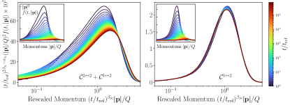
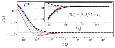
Figure 2: (Top) Gluon distribution function $|\mathbf{p}|^{2}f(t,|\mathbf{p}|)$ from kinetic theory simulation with (left) elastic and inelastic and (right) only inelastic processes rescaled with fixed point exponents $(\alpha_{\infty},\beta_{\infty})=(-4/7,-1/7)$, with $t_{\mathrm{ref}}\,Q\sim 66$. The unrescaled distributions are shown in the insets. (Bottom) Comparison of prescaling exponents from inelastic-only simulations to analytical expectation (5b). We determine $t_{*}=t_{0}(1-\beta_{\infty}/\beta_{0})$ from the data at $t_{0}\,Q\sim 2$ (dashed black line) and at $t_{0}\,Q\sim 10^{4}$ (solid black line). Different colors represent prescaling exponents extracted from different integral moments, see Eq. (A3).

A scaling analysis for the vacuum QCD collision kernel together with energy conservation $\sigma=d+z=4$ reveals the direct energy cascade fixed point $(\alpha_{\infty},\beta_{\infty})=(-4/7,-1/7)$, see [35, 36, 37]. However, the overall scaling of the elastic collision kernel is broken by the presence of the Debye mass $m^{2}_{D}(t)\sim\int d^{3}\mathbf{p}f(t,\mathbf{p})/p\sim A(t)B(t)^{-2}\bar{m}^{2}_{D}$ that regulate soft elastic scatterings where $\bar{m}^{2}_{D}\equiv m^{2}_{D}(t_{0})$, see Eq. (A7). The time-dependent (scaling) Debye mass can not generally be factored from the elastic scattering matrix element, which breaks the assumption of overall scaling behavior of the collision kernel. This breaking of scaling is visualized in the top panel of Fig. 2, where we show $|\mathbf{p}|^{2}f(t,|\mathbf{p}|)$ rescaled with fixed point exponents. The rescaling for simulations with only inelastic scatterings (top right) shows a very clear collapse of all curves from shortly after initialization over an evolution of six orders of magnitude, but a spread cannot be removed for all times even by time dependent rescalings if one includes elastic scatterings (top left) due to the presence of the Debye mass. In the lower panel we extract prescaling exponents for only inelastic scatterings ${\cal C}^{1\leftrightarrow 2}$ from different moments of the distribution function (see Eq. (A3)). The resulting approach of $\beta(t)$ to the fixed point value $\beta_{\infty}=-1/7$ (dashed gray line) is demonstrated to be well-described over more than seven orders of magnitude in time by Eq. (5b) (dashed black line) with $\mu_{\alpha}=3$ and $\mu_{\beta}=-1$, see Eq. (A15), even at surprisingly early times shortly after initialization. In the inset, we show that this solution initialized at a very early time $t_{0}\,Q\sim 2$ with $t_{*}$ obtained from $\beta(t_{0})\equiv\beta_{0}$ captures the evolution at intermediate times $t\,Q\sim 10^{4}$ only qualitatively. If we obtain $t_{*}$ in the same way at a later time $t_{0}\,Q\sim 10^{4}$, Eq. (5b) describes the late-time evolution quantitatively well as given by the solid black line. We do not display $\alpha(t)$ explicitly here and in the following as we find the scaling relation $\alpha(t)/\beta(t)=4$ realized to a very good accuracy.

The conclusion here is that the separation of variables, see Eq. (4), in QCD kinetic theory can thus not generally be performed, as $m_{D}(t)$ leads to a mixing of time and (rescaled) momentum scales in the prescaling regime. With $\alpha_{\infty},\beta_{\infty}<0$, the Debye mass decreases over time such that the violation of scaling becomes increasingly small. These two effects lead to the expectation that different momenta of the distribution function approach the fixed point on different timescales. This is visible already in the top left of Fig. 2, where (rescaled) momenta $\gtrsim 4$ are observed to scale well with fixed point exponents whilst smaller ones do not. We then expect scaling exponents from different moments to converge only asymptotically in the approach to the fixed point. This we corroborate in Fig. 3, where a spread in prescaling exponents obtained from different moments is observed to remain for the latest times reached.

Effect of scaling breaking terms in the Fokker-Planck approximation.– The breaking of scaling inhibits prescaling exponents extracted from different moments to share the same universal prescaling dynamics. Nevertheless, at qualitative level the scaling dynamics can be reasonably modeled via the Fokker-Planck (FP) approximation [38, 39, 40]. This approach assumes the dominance of small angle scatterings and has previously been used in the context of nonthermal attractors [41] and prescaling [19, 20]. We will compare our analytical results from the FP approximation to simulations using the full QCD collision kernel. The corresponding FP collision kernel allows us to factorize the scaling-breaking Coulomb logarithm, which involves the ratio of the UV scale, the characteristic gluon energy $\langle p\rangle$, and the IR scale, the Debye mass $m_{D}$

$${\cal C}^{\mathrm{FP}}[f](t,\mathbf{p}) =\frac{A(t)^{3}}{B(t)}\log\left[\frac{\langle\bar{p}\rangle}{A(t)^{\frac{1}{2}}\bar{m}_{D}}\right]\tilde{C}^{\mathrm{FP}}[f_{S}](\bar{\mathbf{p}}),$$ (6)

where we only display terms relevant for the scaling analysis and refer to Eq. (A18) for details. Upon separating variables with associated constant $D_{2}$, see Eq. (4), and relating $\alpha(t)=\sigma\beta(t)$ as before, we now obtain

$$\partial_{t}B(t)=\frac{\beta_{0}}{t_{0}}B(t)^{2\sigma}\left[1-\frac{\sigma}{2}\frac{\log[B(t)]}{\log[\langle\bar{p}\rangle/\bar{m}_{D}]}\right].$$ (7)

We identified $D_{2}=\beta_{0}/(t_{0}\log[\langle\bar{p}\rangle/\bar{m}_{D}])$, which is an intricate self-consistent equation as $\log[\langle\bar{p}\rangle/\bar{m}_{D}]$ depends implicitly on $D_{2}$ via $f_{S}$, see also the discussion below Eq. (4). We avoid the need to solve it as we utilize our simulations to obtain $\langle\bar{p}\rangle/\bar{m}_{D}$ as a function of $\beta_{0}/t_{0}$.

Equation (7) can be directly integrated, but then $B(t)$ appears as an argument of a nontrivial transcendental function. A more useful approach is to derive from Eq. (7) a second order differential equation for $\beta(t)$

$$\frac{\ddot{\beta}(t)}{\beta(t)}=\frac{\dot{\beta}(t)^{2}}{\beta(t)^{2}}+\frac{14\dot{\beta}}{t}-\frac{(7\beta(t)+1)^{2}}{t^{2}}.$$ (8)

This equation is also subtle, as its second order character stays in contrast with the number of parameters needed to solve Eq. (7), which requires specifying only $\beta_{0}$ at $t_{0}$. Indeed, there is a nontrivial constraint on initial data for Eq. (8) directly following from a derivative of Eq. (7): $\dot{\beta}(t_{0})\equiv\dot{\beta}_{0}=\tfrac{\beta_{0}}{t_{0}}[1-\beta_{0}/\beta_{\infty}-1/\log{\sqrt{\langle\bar{p}\rangle/\bar{m}_{D}}}]$. Its complexity arises from the dependence of $\langle\bar{p}\rangle/\bar{m}_{D}$ on $\beta_{0}$ and $t_{0}$. What one can already see quickly is that $\beta(t)=\beta_{\infty}=-1/7$ is a consistent late time solution of (8), as it satisfies the constraint in the limit $t_{0}\rightarrow\infty$.

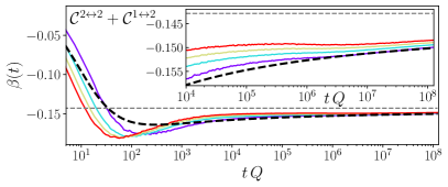
Figure 3: Comparison between prescaling exponents extracted from QCD kinetic theory simulations with scaling-breaking elastic processes (see Fig. 2 (top left)) and the analytical prescaling expectation of Eq. (8) (dashed black line).

In Fig. 3 the evolution of $\beta(t)$ extracted from QCD kinetic theory (solid color lines) is shown to be captured well by Eq. (8) (dashed black line) from times shortly after initialization of the system over more than seven orders of magnitude. We obtain this result by solving Eq. (8) with initial condition at $t_{0}$ for $\dot{\beta}_{0}$ determined by the constraint and $\beta_{0}$ (as well as $\log\sqrt{\langle\bar{p}\rangle/\bar{m}_{D}}$) extracted from the data. In the inset we show that solving Eq. (8) shortly after initialization also describes the late-time dynamics qualitatively well, where the prescaling exponents from different moments retain a finite spread for the latest simulated times.

We now want to understand the prescaling dynamics in the vicinity of the fixed point. We can linearize Eq. (8) in perturbations $\delta\beta(t)$ around the fixed point value $\beta_{\infty}=-1/7$, which yields a power-law decay from below $\delta\beta(t)\sim-1/t$. On top of this, the slow part of the solution to Eq. (8) is

$$\beta(t) \approx \beta_{\infty}+\sum_{m=1}^{\infty}\sum_{n=0}^{m-1}\beta_{m,n}\frac{\log(\log(t\,Q))^{n}}{\log(t\,Q)^{m}}$$ (9a)

$$\approx \beta_{\infty}\left[1+\frac{1}{\log(t\,Q)}\right],$$ (9b)

where we used $Q$ as the reference scale but emphasize that the choice of a constant does not matter at late enough times. This logarithmic correction is a non-linear effect not captured by the linearization procedure. Similar late-time power-law [20] corrections from linearization and late-time logarithmic [19] corrections induced by the temporal evolution of the Coulomb logarithm were found for the Baier-Mueller-Schiff-Son [12] fixed point in longitudinal expanding plasma.

The simple power-law approach to the fixed point found in the absence of scaling breaking terms in Eq. (5b) is therefore enriched to involve both fast (power-law) and slow (inverse powers of logarithms and slower) behavior. This discussion is reminiscent of the transseries form [42, 43] for late time dynamics of the energy-momentum tensor of matter undergoing longitudinal boost-invariant expansion [44, 45, 46, 47]. There slow modes came from relativistic hydrodynamics and exponentially faster modes from transient excitations. Here slow modes come from the Debye mass breaking the homogeneity of the collision kernel with respect to rescalings of momenta and fast modes are the original prescaling excitations encountered already in (5b). Similarly to [44, 45, 46, 47], it is not difficult to gather finite order indications that the series containing slow modes (9a) is likely to have a vanishing radius of convergence with $\beta_{m+1,0}/\beta_{m,0}\sim m$. Curiously, the leading (at each $m$) doubly logarithmic term behaves geometrically: $\beta_{m+1,m}/\beta_{m,m-1}=-1$. It would be interesting to develop systematic understanding of this behavior, including resummations of the resulting transseries.

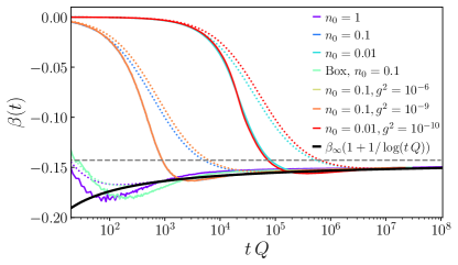
Figure 4: Comparison of prescaling trajectories in QCD kinetic theory simulations. Solid lines correspond to prescaling exponents extracted from simulations with different initial conditions, where for visibility only results from the first moment are displayed. Dotted color lines are solutions to Eq. (8) with initial conditions obtained from these different simulations.

In Fig. 4 we visualize the attractive nature of the prescaling dynamics by extracting prescaling exponents from different initial conditions (solid color lines) and corresponding solutions to Eq. (8) (dotted color lines). All simulations are initialized with variations in parameters of the class of initial condition used in this work apart from the data represented by green, which uses box initial conditions $f(t_{i},\mathbf{p})=n_{0}/g^{2}\theta(Q-|\mathbf{p}|)$. Comparing solid and dotted lines of the same color, we observe that the slow approach to the fixed point value from below is described well by Eq. (8) in accordance with the discussion for Fig. 3. Deviations are observed at early times with $\beta(t)$ approaching the fixed point value initially from above, where Eq. (8) captures the fast dynamics in the fall-off region only qualitatively. Finally, the prescaling exponents extracted from different simulations and the corresponding solutions to Eq. (8) are all found to converge to a universal late-time behavior, which we additionally show is well described by Eq. (9b) (solid black line). Furthermore, we want to emphasize the similarity between the behavior shown in Fig. 4 and hydrodynamic attractors, where different solutions converge to a single universal curve which at sufficiently late times is described by relativistic hydrodynamics [44, 48, 49].

The above analysis has an important bearing on the appearance of scaling. The regime when the highest order terms in the collision kernel dominate parametrically ends when the typical occupancy becomes of $\mathcal{O}(1)$. This is realized if $t_{f}Q\geq\alpha^{-7/4}_{S}$ [13]. At that time, we have a deviation of $\delta\beta(t)/\beta\sim 1/\log(\alpha^{-7/4}_{S})\lesssim 0.03$ with $g^{2}=10^{-8}$. As a consequence of this, the system will therefore still show percent deviations from the fixed point values when the direct energy cascade ceases and ultraviolet modes $|\mathbf{p}|/Q\geq 1$ start to thermalize.

Conclusions.– We studied the approach of isotropic and spatially homogeneous quantum many-body systems to nonthermal attractors. Our results demonstrate that the prescaling is governed by a simple first-order ordinary differential equation obtained from the underlying dynamics via emergent conservation laws.

Our analytical prediction implies that prescaling entails infinitely many power-law corrections to constant scaling exponents. They conspire to a simple time off-set in the fixed point scaling. We have successfully tested our simple formula for prescaling against ab initio simulations of a vector model relativistic QFT using 2PI formalism and QCD kinetic theory simulations. Our QCD kinetic theory simulations span eight orders of magnitude in time and provide the most accurate extraction of scaling exponents to date.

The exact scaling associated with nonthermal attractors requires the collision term to be a homogeneous functional of particle momenta at large occupations. For QCD kinetic theory this property is violated by the Debye mass term that regulates the Coulomb divergence in the elastic scattering matrix element. We demonstrate that exact scaling exponents are not reached during the lifetime of the system. Using the Fokker-Planck approximation to QCD kinetic theory we show that the scaling-breaking Couloumb logarithm significantly enriches the prescaling dynamics. The late-time behavior is given by a factorial divergent series that includes inverse powers of logarithms and positive powers of double logarithms of time. This constitutes a striking structural similarity with theoretical descriptions of hydrodynamic attractors in the boost-invariant models of nuclear collisions.

Our work shows that prescaling is an unavoidable consequence of nonthermal attractors. Therefore our analytical predictions for prescaling can be verified experimentally in cold atom systems. Furthermore, we uncovered that scaling breaking terms generate rich prescaling dynamics that bares similarities to transseries in the context of hydrodynamic attractors. It would be fascinating to utilize the enormous degree of control in cold atom systems to induce scaling breaking terms and experimentally discover the phenomenology of transseries.

Acknowledgments.– We thank I. Aniceto, J. Berges, K. Boguslavski, J. Brewer, A. Kurkela, A. Mikheev, J. Noronha, B. Scheihing-Hitschfeld, S. Schlichting, A. Serantes, R. Venugopalan, and Y. Yin for useful discussions and comments on the draft. The authors acknowledge support by the state of Baden-Württemberg through bwHPC and the German Research Foundation (DFG) through grant no INST 40/575-1 FUGG (JUSTUS 2 cluster), and DFG under the Collaborative Research Center SFB 1225 ISOQUANT (Project-ID 27381115) and the Heidelberg STRUCTURES Excellence Cluster under Germany’s Excellence Strategy EXC2181/1-390900948. The work of AM is funded by DFG – Project number 496831614. We would like to thank KITP for its hospitality during the program “The Many Faces of Relativistic Fluid Dynamics” supported by the National Science Foundation under Grant No. NSF PHY-1748958.

Appendix A Appendix

A.1 Extraction of scaling exponents

Under the prescaling ansatz for an isotropic system, Eq. (2), we introduce moments of the distribution function

$$n_{m}(t) =\int\frac{d^{d}\mathbf{p}}{(2\pi)^{d}}|\mathbf{p}|^{m}f(t,\mathbf{p})=A(t)B(t)^{-(d+m)}\bar{n}_{m},$$ (A1)

whose evolutions are given by the dynamics of prescaling exponents [17]

$$\frac{d}{d\log t}\log(n_{m}(t))=\alpha(t)-(d+m)\beta(t).$$ (A2)

We can thus extract prescaling exponents from the evolution of the moments, for example,

$$\alpha_{m}(t)=(m+d)(m+1+d)\frac{d}{d\log t}\log\left[\frac{n^{\frac{1}{m+d}}_{m}(t)}{n^{\frac{1}{m+1+d}}_{m+1}(t)}\right],\qquad\beta_{m}(t)=\frac{d}{d\log t}\log\left(\frac{n_{m}(t)}{n_{m+1}(t)}\right).$$ (A3)

We can similarly obtain the general $A(t)$ and $B(t)$ from the moments of the distribution function (or equivalently from moments of the equal-time statistical function $F(t,t,|\mathbf{p}|)$ for the inverse cascade fixed point) according to

$$A(t)=\left[\frac{n^{1/(d+m)}_{m}(t)}{n^{1/(d+m+1)}_{m+1}(t)}\frac{\bar{n}^{1/(d+m+1)}_{m+1}(t)}{\bar{n}^{1/(d+m)}_{m}}\right]^{(d+m)(d+m+1)},\hskip 71.13188ptB(t)=\frac{n_{m}(t)}{n_{m+1}(t)}\frac{\bar{n}_{m+1}}{\bar{n}_{m}},$$ (A4)

where $\bar{n}_{m}\equiv n_{m}(t_{0})$ such that $B(t_{0})=1$.

A.2 QCD kinetic theory and prescaling

In this work we study QCD kinetic theory which includes $2\leftrightarrow 2$ and $1\leftrightarrow 2$ collinear scattering terms. We will give the corresponding equations for the gluon sector here and refer to [27, 1] for the complete expressions including other particle species. The gluon collision kernels are parametrized as

$$C^{2\leftrightarrow 2}[f](t,\mathbf{p}) =-\frac{1}{8p(N^{2}_{c}-1)}\int\frac{d^{3}\mathbf{k}d^{3}\mathbf{p}^{\prime}d^{3}\mathbf{k}^{\prime}}{(2\pi)^{9}2k2p^{\prime}2k^{\prime}}|\mathcal{M}^{gg}_{gg}|^{2}(p,k,p^{\prime},k^{\prime})(2\pi)^{4}\delta^{(4)}(p^{\mu}+k^{\mu}-p^{\prime\mu}-k^{\prime\mu})$$

$$\times\left[f_{\mathbf{p}}f_{\mathbf{k}}(1+f_{\mathbf{k}^{\prime}})(1+f_{\mathbf{p}^{\prime}})-f_{\mathbf{p}^{\prime}}f_{\mathbf{k}^{\prime}}(1+f_{\mathbf{p}})(1+f_{\mathbf{k}})\right]$$ (A5a)

$$C^{1\leftrightarrow 2}[f](t,\mathbf{p}) =-\frac{(2\pi)^{3}}{8p^{2}(N^{2}_{c}-1)}\int_{0}^{\infty}dp^{\prime}dk^{\prime}\left\{\gamma^{g}_{gg}(p;p^{\prime},k^{\prime})\delta^{(1)}(p-p^{\prime}-k^{\prime})\left[f_{p\hat{\mathbf{p}}}(1+f_{p^{\prime}\hat{\mathbf{p}}})(1+f_{k^{\prime}\hat{\mathbf{p}}})-f_{p^{\prime}\hat{\mathbf{p}}}f_{k^{\prime}\hat{\mathbf{p}}}(1+f_{p\hat{\mathbf{p}}})\right]\right.$$

$$\left.-2\gamma^{g}_{gg}(p^{\prime};p,k^{\prime})\delta^{(1)}(p^{\prime}-p-k^{\prime})\left[f_{p^{\prime}\hat{\mathbf{p}}}(1+f_{p\hat{\mathbf{p}}})(1+f_{k^{\prime}\hat{\mathbf{p}}})-f_{p\hat{\mathbf{p}}}f_{k^{\prime}\hat{\mathbf{p}}}(1+f_{p^{\prime}\hat{\mathbf{p}}})\right]\right\},$$ (A5b)

where we used the abbreviations $f_{\mathbf{p}}=f(t,\mathbf{p})$, $p=|\mathbf{p}|$, and $\hat{\mathbf{p}}=\mathbf{p}/p$ is the direction of collinear splitting with corresponding rate $\gamma^{g}_{gg}$. $|\mathcal{M}^{gg}_{gg}|^{2}$ is the $2\leftrightarrow 2$ scattering matrix element averaged over spin and color degrees of freedom. In vacuum, the corresponding expression [25]

$$|\mathcal{M}^{gg}_{gg}|^{2}(p,k,p^{\prime},k^{\prime})=16(N^{2}_{c}-1)N^{2}_{c}g^{4}\left(3-\frac{s_{M}t_{M}}{u^{2}_{M}}-\frac{s_{M}u_{M}}{t^{2}_{M}}-\frac{t_{M}u_{M}}{s^{2}_{M}}\right)$$ (A6)

contains an infrared divergent term $(u_{M}-s_{M})/t_{M}\sim 1/q^{2}$ (also in the $u_{M}$-channel) with $q$ the $t_{M}$-channel momentum transfer for a soft gluon exchange and $u_{M},s_{M},t_{M}$ denote the usual Mandelstam variables. This is regulated by inclusion of necessary physical interactions with the medium, where the leading thermal corrections are obtained as [37, 27]

$$\frac{u_{M}-s_{M}}{t_{M}}\to\frac{u_{M}-s_{M}}{t_{M}}\frac{q^{2}}{q^{2}+\xi^{2}_{g}m^{2}_{D}(t)}=\frac{\bar{u}_{M}-\bar{s}_{M}}{\bar{t}_{M}}\frac{\bar{q}^{2}}{\bar{q}^{2}+\xi^{2}_{g}A(t)\bar{m}^{2}_{D}}$$ (A7)

with $\xi_{g}=e^{5/6}/2$. The inclusion of screening effects however makes the scattering matrix element not invariant under rescaling as indicated due to different scaling of the Debye mass

$$m^{2}_{D}=2g^{2}N_{c}\int\frac{d^{3}\mathbf{p}}{(2\pi)^{3}p}f(t,\mathbf{p})=A(t)B(t)^{-2}\bar{m}^{2}_{D}.$$ (A8)

Moreover, the time-dependent Debye mass enters the scattering matrix element via Eq. (A7) in the denominator such that it can not be factored out thereby violating the assumption of overall scaling for the elastic collision kernel.

We now show that the inelastic collision kernel (A5b) scales with $\mu_{\alpha}=3$ and $\mu_{\beta}=-1$ under prescaling in the non-expanding system (2). We consider only the first term since both have the same scaling behavior. Crucially, we need to know the scaling behavior of the splitting rate, which can be extracted from its two prevalent limiting regimes for soft gluon radition $z=p^{\prime}/p\ll 1$: the Bethe-Heitler (BH) limit in which interferences between successive scatterings are negligible and the Landau-Pomeranchuk-Migdal (LPM) limit in which successive scattering events by the medium interfere destructively. The rate in the respective limit reads

$$\gamma^{g}_{gg}(p;p^{\prime},k^{\prime})|^{z\ll 1}_{\mathrm{BH}}\sim\frac{\hat{q}(\mu)p}{m^{2}_{D}}|_{\mu=em_{D}},\qquad\gamma^{g}_{gg}(p;p^{\prime},k^{\prime})|^{z\ll 1}_{\mathrm{LPM}}\sim\sqrt{\hat{q}(\mu)p},$$ (A9)

where we only included those terms relevant for a scaling analysis with diffusion coefficient

$$\hat{q}(\mu)\sim\log\frac{\mu^{2}}{2m^{2}_{D}}\int\frac{d^{3}\mathbf{p}}{(2\pi)^{3}}f_{\mathbf{p}}(1+f_{\mathbf{p}})\simeq\log\frac{\mu^{2}}{2A(t)B(t)^{-2}\bar{m}^{2}_{D}}A(t)^{2}B(t)^{-3}\int\frac{d^{3}\bar{\mathbf{p}}}{(2\pi)^{3}}f_{S,\bar{\mathbf{p}}}f_{S,\bar{\mathbf{p}}}$$ (A10)

in this overoccupied scenario. For $\hat{q}(\mu)|_{\mu=em_{D}}$ in the BH limit, we thus have $\hat{q}(\mu)=A(t)^{2}B(t)^{-3}\bar{\hat{q}}$ and

$$\gamma^{g}_{gg}(p;p^{\prime},k^{\prime})|^{z\ll 1}_{\mathrm{BH}}\sim\frac{A(t)^{2}B(t)^{-3}\bar{\hat{q}}B(t)^{-1}\bar{p}}{A(t)B(t)^{-2}\bar{m}_{D}}\sim A(t)B(t)^{-2}(t)\bar{\gamma}^{g}_{gg}|^{z\ll 1}_{\mathrm{BH}}.$$ (A11)

For the LPM limit, $\mu$ is to next-to-leading-logarithmic order given self-consistently via

$$\mu^{2}\sim\sqrt{\hat{q}(\mu)p}\sim\sqrt{A(t)^{2}B(t)^{-3}\log\left(\frac{\mu^{2}}{2A(t)B(t)^{-2}\bar{m}^{2}_{D}}\right)B(t)^{-1}}\sim A(t)B(t)^{-2}\sqrt{\log\left(\frac{\mu^{2}}{2A(t)B(t)^{-2}\bar{m}^{2}_{D}}\right)},$$ (A12)

which show that $\mu$ scales self-consistently as $\mu^{2}\sim A(t)B(t)^{-2}$ such that the time dependence drops out of $\log(\mu^{2}/(2m^{2}_{D}))$. Accordingly, for the LPM limit we thus find again

$$\gamma^{g}_{gg}(p;p^{\prime},k^{\prime})|^{z\ll 1}_{\mathrm{LPM}}\sim\sqrt{\hat{q}(\mu)p}\sim\sqrt{A(t)^{2}B(t)^{-3}\bar{\hat{q}}(\mu)B(t)^{-1}\bar{p}}\sim A(t)B(t)^{-2}\hat{\gamma}^{g}_{gg}|^{z\ll 1}_{\mathrm{LPM}}$$ (A13)

The rate therefore scales like the Debye mass in both limits and we will adopt this scaling for the complete rate $\gamma^{g}_{gg}\sim A(t)B(t)^{-2}\bar{\gamma}^{g}_{gg}$. This leads to the overall scaling prediction

$$C^{1\leftrightarrow 2}[f](t,\mathbf{p}) \sim\frac{1}{B(t)^{-2}\bar{p}^{2}}\int_{0}^{\infty}B(t)^{-2}d\bar{p}^{\prime}d\bar{k}^{\prime}A(t)B(t)^{-2}\bar{\gamma}^{g}_{gg}(\bar{p};\bar{p}^{\prime},\bar{k}^{\prime})B(t)\delta^{(1)}(\bar{p}-\bar{p}^{\prime}-\bar{k}^{\prime})$$

$$\qquad\qquad\qquad\times A(t)^{2}\left[f_{S,\bar{p}\bar{\hat{\mathbf{p}}}}(f_{S,\bar{p}^{\prime}\bar{\hat{\mathbf{p}}}}+f_{\bar{k}^{\prime}\bar{\hat{\mathbf{p}}}})-f_{S,\bar{p}^{\prime}\bar{\hat{\mathbf{p}}}}f_{S,\bar{k}^{\prime}\bar{\hat{\mathbf{p}}}}\right]$$ (A14)

$$\sim A(t)^{3}B(t)^{-1}C^{1\leftrightarrow 2}[f_{S}](\bar{\mathbf{p}})$$ (A15)

such that we can identify $\mu_{\alpha}=3$ and $\mu_{\beta}=-1$ as anticipated. $C^{1\leftrightarrow 2}$ will therefore lead to the direct energy cascade fixed point $(\alpha_{\infty},\beta_{\infty})=(-4/7,-1/7)$ as we demonstrate in Fig. 2 of the main text.
The scaling analysis for the elastic collision kernel in the absence of the Debye mass has been performed in [36] and can simply be generalized to the prescaling case with again $\mu_{\alpha}=3$ and $\mu_{\beta}=-1$. This scaling analysis however needs to be augmented by the inclusion of the Debye mass as we discussed above, which leads to an effective regulation of the divergent soft contributions to the elastic collision kernel and prevents one from extracting an overall scaling behavior thereof.

A.3 Fokker-Planck approximation

We assume the gluons to interact via elastic small-angle scatterings such that the collision kernel takes a FP form [38, 40, 1, 19]

$$C^{\mathrm{FP}}(t,\mathbf{p}) \sim\ln\frac{\langle p\rangle(t)}{m_{D}(t)}\left[\int\frac{d^{3}\mathbf{k}}{(2\pi)^{3}}f_{\mathbf{k}}(1+f_{\mathbf{k}})\;\partial^{2}_{p}f_{\mathbf{p}}+\int\frac{d^{3}\mathbf{k}}{(2\pi)^{3}k}2f_{\mathbf{k}}\;\vec{\nabla}_{\mathbf{p}}\cdot\left(\frac{\mathbf{p}}{p}(1+f_{\mathbf{p}})f_{\mathbf{p}}\right)\right]$$ (A16)

$$\equiv\ln\frac{\langle p\rangle(t)}{m_{D}(t)}\tilde{C}^{\mathrm{FP}}[f](t,\mathbf{p}),$$ (A17)

where we highlighted the contributions relevant for a scaling analysis and here $\langle\dots\rangle\equiv\int\frac{d^{3}\mathbf{p}}{(2\pi)^{3}}\dots f(t,\mathbf{p})/\int\frac{d^{3}\mathbf{p}}{(2\pi)^{3}}f(t,\mathbf{p})$. The advantage of the FP approximation for a prescaling analysis becomes apparent here, as the contribution due to the Debye mass in the elastic QCD scattering matrix element is simply factorized into a logarithm of the characteristic UV and IR scale. Plugging in the prescaling ansatz, we then find directly that

$$C^{\mathrm{FP}}[f](t,\mathbf{p}) =\ln\left[\frac{\langle\bar{p}\rangle}{A(t)^{\tfrac{1}{2}}\bar{m}_{D}}\right]A(t)^{3}B(t)^{-1}\tilde{C}^{\mathrm{FP}}[f_{S}](\bar{\mathbf{p}}).$$ (A18)

References

- Berges et al. [2021] J. Berges, M. P. Heller, A. Mazeliauskas, and R. Venugopalan, Rev. Mod. Phys. 93, 035003 (2021), arXiv:2005.12299 [hep-th] .
- Prüfer et al. [2018] M. Prüfer, P. Kunkel, H. Strobel, S. Lannig, D. Linnemann, C.-M. Schmied, J. Berges, T. Gasenzer, and M. K. Oberthaler, Nature 563, 217 (2018), arXiv:1805.11881 [cond-mat.quant-gas] .
- Erne et al. [2018] S. Erne, R. Bücker, T. Gasenzer, J. Berges, and J. Schmiedmayer, Nature 563, 225 (2018), arXiv:1805.12310 [cond-mat.quant-gas] .
- Glidden et al. [2021] J. A. P. Glidden, C. Eigen, L. H. Dogra, T. A. Hilker, R. P. Smith, and Z. Hadzibabic, Nature Phys. 17, 457 (2021), arXiv:2006.01118 [cond-mat.quant-gas] .
- Navon et al. [2016] N. Navon, A. L. Gaunt, R. P. Smith, and Z. Hadzibabic, Nature 539, 72 (2016), arXiv:1609.01271 [cond-mat.quant-gas] .
- Johnstone et al. [2019] S. P. Johnstone, A. J. Groszek, P. T. Starkey, C. J. Billington, T. P. Simula, and K. Helmerson, Science 364, 1267 (2019), ”https://www.science.org/doi/pdf/10.1126/science.aat5793” .
- Helmrich et al. [2020] S. Helmrich, A. Arias, G. Lochead, T. Wintermantel, M. Buchhold, S. Diehl, and S. Whitlock, Nature 577, 481 (2020), arXiv:1806.09931 [cond-mat.quant-gas] .
- García-Orozco et al. [2022] A. D. García-Orozco, L. Madeira, M. A. Moreno-Armijos, A. R. Fritsch, P. E. S. Tavares, P. C. M. Castilho, A. Cidrim, G. Roati, and V. S. Bagnato, Phys. Rev. A 106, 023314 (2022), arXiv:2107.07421 [cond-mat.quant-gas] .
- Martirosyan et al. [2023] G. Martirosyan, C. J. Ho, J. Etrych, Y. Zhang, A. Cao, Z. Hadzibabic, and C. Eigen, (2023), arXiv:2304.06697 [cond-mat.quant-gas] .
- Huh et al. [2023] S. Huh, K. Mukherjee, K. Kwon, J. Seo, S. I. Mistakidis, H. R. Sadeghpour, and J.-y. Choi, (2023), arXiv:2303.05230 [cond-mat.quant-gas] .
- Lannig et al. [2023] S. Lannig, M. Prüfer, Y. Deller, I. Siovitz, J. Dreher, T. Gasenzer, H. Strobel, and M. K. Oberthaler, (2023), arXiv:2306.16497 [cond-mat.quant-gas] .
- Baier et al. [2001] R. Baier, A. H. Mueller, D. Schiff, and D. T. Son, Phys. Lett. B 502, 51 (2001), arXiv:hep-ph/0009237 .
- Berges et al. [2014a] J. Berges, K. Boguslavski, S. Schlichting, and R. Venugopalan, Phys. Rev. D 89, 074011 (2014a), arXiv:1303.5650 [hep-ph] .
- Kurkela and Zhu [2015] A. Kurkela and Y. Zhu, Phys. Rev. Lett. 115, 182301 (2015), arXiv:1506.06647 [hep-ph] .
- Micha and Tkachev [2003] R. Micha and I. I. Tkachev, Phys. Rev. Lett. 90, 121301 (2003), arXiv:hep-ph/0210202 .
- Berges et al. [2008] J. Berges, A. Rothkopf, and J. Schmidt, Phys. Rev. Lett. 101, 041603 (2008), arXiv:0803.0131 [hep-ph] .
- Mazeliauskas and Berges [2019] A. Mazeliauskas and J. Berges, Phys. Rev. Lett. 122, 122301 (2019), arXiv:1810.10554 [hep-ph] .
- Mikheev et al. [2019] A. N. Mikheev, C.-M. Schmied, and T. Gasenzer, Phys. Rev. A 99, 063622 (2019), arXiv:1807.10228 [cond-mat.quant-gas] .
- Brewer et al. [2022] J. Brewer, B. Scheihing-Hitschfeld, and Y. Yin, JHEP 05, 145 (2022), arXiv:2203.02427 [hep-ph] .
- Mikheev et al. [2022] A. N. Mikheev, A. Mazeliauskas, and J. Berges, Phys. Rev. D 105, 116025 (2022), arXiv:2203.02299 [hep-ph] .
- Preis et al. [2023] T. Preis, M. P. Heller, and J. Berges, Phys. Rev. Lett. 130, 031602 (2023), arXiv:2209.14883 [hep-ph] .
- Piñeiro Orioli et al. [2015] A. Piñeiro Orioli, K. Boguslavski, and J. Berges, Phys. Rev. D 92, 025041 (2015), arXiv:1503.02498 [hep-ph] .
- Micha and Tkachev [2004] R. Micha and I. I. Tkachev, Phys. Rev. D 70, 043538 (2004), arXiv:hep-ph/0403101 .
- Walz et al. [2018] R. Walz, K. Boguslavski, and J. Berges, Phys. Rev. D 97, 116011 (2018), arXiv:1710.11146 [hep-ph] .
- Arnold et al. [2003] P. B. Arnold, G. D. Moore, and L. G. Yaffe, JHEP 01, 030 (2003), arXiv:hep-ph/0209353 .
- Keegan et al. [2016] L. Keegan, A. Kurkela, A. Mazeliauskas, and D. Teaney, JHEP 08, 171 (2016), arXiv:1605.04287 [hep-ph] .
- Kurkela and Mazeliauskas [2019] A. Kurkela and A. Mazeliauskas, Phys. Rev. D 99, 054018 (2019), arXiv:1811.03068 [hep-ph] .
- Berges et al. [2015] J. Berges, K. Boguslavski, S. Schlichting, and R. Venugopalan, Phys. Rev. Lett. 114, 061601 (2015), arXiv:1408.1670 [hep-ph] .
- Deng et al. [2018] J. Deng, S. Schlichting, R. Venugopalan, and Q. Wang, Phys. Rev. A 97, 053606 (2018), arXiv:1801.06260 [hep-th] .
- Chantesana et al. [2019] I. Chantesana, A. Piñeiro Orioli, and T. Gasenzer, Phys. Rev. A 99, 043620 (2019), arXiv:1801.09490 [cond-mat.quant-gas] .
- Piñeiro Orioli and Berges [2019] A. Piñeiro Orioli and J. Berges, Phys. Rev. Lett. 122, 150401 (2019), arXiv:1810.12392 [cond-mat.quant-gas] .
- Schmied et al. [2019] C.-M. Schmied, A. N. Mikheev, and T. Gasenzer, Phys. Rev. Lett. 122, 170404 (2019), arXiv:1807.07514 [cond-mat.quant-gas] .
- Boguslavski and Piñeiro Orioli [2020] K. Boguslavski and A. Piñeiro Orioli, Phys. Rev. D 101, 091902 (2020), arXiv:1911.04506 [hep-ph] .
- Boguslavski et al. [2022] K. Boguslavski, T. Lappi, M. Mace, and S. Schlichting, Phys. Lett. B 827, 136963 (2022), arXiv:2106.11319 [hep-ph] .
- Schlichting [2012] S. Schlichting, Phys. Rev. D 86, 065008 (2012), arXiv:1207.1450 [hep-ph] .
- Berges et al. [2014b] J. Berges, K. Boguslavski, S. Schlichting, and R. Venugopalan, Phys. Rev. D 89, 114007 (2014b), arXiv:1311.3005 [hep-ph] .
- Abraao York et al. [2014] M. C. Abraao York, A. Kurkela, E. Lu, and G. D. Moore, Phys. Rev. D 89, 074036 (2014), arXiv:1401.3751 [hep-ph] .
- Mueller [2000] A. H. Mueller, Phys. Lett. B 475, 220 (2000), arXiv:hep-ph/9909388 .
- Blaizot et al. [2013] J.-P. Blaizot, J. Liao, and L. McLerran, Nucl. Phys. A 920, 58 (2013), arXiv:1305.2119 [hep-ph] .
- Schlichting and Teaney [2019] S. Schlichting and D. Teaney, Ann. Rev. Nucl. Part. Sci. 69, 447 (2019), arXiv:1908.02113 [nucl-th] .
- Tanji and Venugopalan [2017] N. Tanji and R. Venugopalan, Phys. Rev. D 95, 094009 (2017), arXiv:1703.01372 [hep-ph] .
- Dorigoni [2019] D. Dorigoni, Annals Phys. 409, 167914 (2019), arXiv:1411.3585 [hep-th] .
- Aniceto et al. [2019a] I. Aniceto, G. Basar, and R. Schiappa, Phys. Rept. 809, 1 (2019a), arXiv:1802.10441 [hep-th] .
- Heller and Spalinski [2015] M. P. Heller and M. Spalinski, Phys. Rev. Lett. 115, 072501 (2015), arXiv:1503.07514 [hep-th] .
- Basar and Dunne [2015] G. Basar and G. V. Dunne, Phys. Rev. D 92, 125011 (2015), arXiv:1509.05046 [hep-th] .
- Aniceto and Spaliński [2016] I. Aniceto and M. Spaliński, Phys. Rev. D 93, 085008 (2016), arXiv:1511.06358 [hep-th] .
- Aniceto et al. [2019b] I. Aniceto, B. Meiring, J. Jankowski, and M. Spaliński, JHEP 02, 073 (2019b), arXiv:1810.07130 [hep-th] .
- Romatschke [2018] P. Romatschke, Phys. Rev. Lett. 120, 012301 (2018), arXiv:1704.08699 [hep-th] .
- Jankowski and Spaliński [2023] J. Jankowski and M. Spaliński, Prog. Part. Nucl. Phys. 132, 104048 (2023), arXiv:2303.09414 [nucl-th] .