Azimuthal temperature variations in ISO-Oph 2 from multi-frequency ALMA observations

Abstract

Environmental effects, such as stellar fly-bys and external irradiation, are thought to affect the evolution of protoplanetary disks in clustered star formation. Previous ALMA images at 225 GHz of the ISO-Oph 2 binary revealed a peculiar morphology in the disk of the primary, perhaps due to a possible fly-by with the secondary. Here we report on new ALMA continuum observations of this system at 97.5 GHz, 145 GHz and 405 GHz, which reveal strong morphological variations. Multi-frequency positional alignment allows to interpret these spectral variations in terms of underlying physical conditions. ISO-Oph 2A is remarkably offset from the centroid of its ring, at all frequencies, and the disk is lopsided, pointing at gravitational interactions. However, the dust temperature also varies in azimuth, with two peaks whose direction connects with HD 147889, the earliest-type star in the Ophiuchus complex, suggesting that it is the dominant heat source. The stellar environment of ISO-Oph 2 appears to drive both its density structure and its thermal balance.

1 Introduction

Interferometric observations at (sub)-millimeter wavelengths can resolve circumstellar disks at subarcsecond resolution and trace the thermal continuum emission due to dust (e.g. Andrews et al., 2009, 2010; Isella et al., 2009). Also, multi-wavelength (sub)-millimeter data can help constrain dust properties such as the maximum grain size (Guilloteau et al., 2011). With unprecedented capabilities, the Atacama Large Millimetre/sub-millimeter Array (ALMA) has revolutionized the field over the last decade. ALMA has already surveyed most star-forming regions in nearby (distances $d<300$ pc) molecular clouds, including Chameleon (Pascucci et al., 2016; Villenave et al., 2021), Lupus (Ansdell et al., 2016, 2018), Taurus (Long et al., 2018, 2019), and Ophiuchus (Cox et al., 2017; Cieza et al., 2019). Even though these surveys have mostly been carried out in a single frequency at a modest resolution (0$\aas@@fstack{\prime\prime}$1 - 0$\aas@@fstack{\prime\prime}$2), they still allow us to investigate disk properties as a function of different variables, such as IR Class (Williams et al., 2019), stellar mass (Barenfeld et al., 2016; Pascucci et al., 2016), age (Ansdell et al., 2018; Ruíz-Rodríguez et al., 2018), and stellar-multiplicity (Cox et al., 2017; Zurlo et al., 2020, 2021).

In models of clustered star formation, the stellar environment affects disk structure and evolution (e.g. Haworth, 2021; Winter & Haworth, 2022; Wilhelm et al., 2023), both through external irradiation, which may lead to photo-evaporation, and through gravitational interaction, including disk truncation and accretion bursts. The Orion proplyds (O’dell & Wen, 1994) are spectacular examples of the impact of environment through external photo-evaporation. Demographic surveys in the Orion nebula cluster show that disk structure is determined in part by the distance to $\theta^{1}$ Ori C (Mann et al., 2014; Eisner et al., 2018). In turn, models of flybys may explain the structures seen in several binary disks (e.g. Dong et al., 2022; Cuello et al., 2023). However, the probability for witnessing such close encounters (with a crossing time of $\lesssim 400$ yr within 500 au at a typical relative velocity of $\sim$6 km s^-1) is very small compared to the disk lifetime ($\sim$10 Myr), and isolated spiral systems haven been shown not to have undergone recent stellar encounters (Shuai et al., 2022, in the past $10^{4}$ yr). In any case, whichever the mechanism, the environment bears a significant role in exoplanet demographics (Winter et al., 2020; Longmore et al., 2021).

The demographic surveys also allow us to identify particularly interesting targets for follow-up studies. Such is the case for the ISO-Oph 2 system, a wide separation (240 au) binary targeted by the Ophiuchus DIsc Survey Employing ALMA (ODISEA, Cieza et al., 2019) in band-6 (230 GHz). ISO-Oph 2 was observed at 0$\aas@@fstack{\prime\prime}$02 resolution, also in band-6, as part of the high-resolution follow-up of the brightest ODISEA targets (Cieza et al., 2021). The high-resolution observation showed that the disk around the primary consists of two non-axisymmetric rings and that the disk around the secondary is a narrow ring with a 2 au inner radius and a 1 au width (González-Ruilova et al., 2020). Furthermore, the ¹²CO data show a bridge of gas connecting both disks, suggesting that the binary is interacting, and is perhaps in a flyby orbit.

Another particularly interesting aspect of ISO-Oph 2 is that, among the long-baseline ODISEA sample (Cieza et al., 2021), it is the closest to HD 147889 (B2IV, B3IV, Casassus et al., 2008), the earliest-type star in the Ophiuchus complex. This proximity raises a question on the role of external irradiation in the thermal balance in the outer ring of ISO-Oph 2. ISO-Oph 2 is thus an interesting case-study for the effect of the stellar environment on protoplanetary disk evolution, both in gravitational interactions and external irradiation.

The ODISEA project has recently been extended to multi-frequency observations covering over 90 objects in ALMA Band-4 (at 145 GHz, Chavan et al. in prep) and Band-8 (405 GHz, Bhowmik et al. in prep.; Cieza et al. in prep) in order to better constrain the physical properties of the Ophiuchus disks when combined with existing data. A crucial aspect of such an analysis is the alignment of the multi-frequency data, which might not be acquired with the same phase center, or could be affected by pointing errors, that could bias spectral trends such as spectral index maps. Casassus & Cárcamo (2022) proposed a strategy for the alignment of multi-epoch and multi-configuration radio-interferometric data, although their application was restricted to the same correlator setups. It is interesting to investigate whether the same strategy might be applied to multi-frequency data.

A crucial aspect of image synthesis is the process of image restoration, which conveys imaging residuals in the final images, along with a well-defined angular resolution. In the last couple of years a technique, usually referred to as the “JvM correction”, has recently been incorporated in image restoration (Jorsater & van Moorsel, 1995; Czekala et al., 2021). The JvM correction reduces the noise and residuals in the final images. Here we stress that the present analysis does not make us of this technique, as the resulting improvement in dynamic range is spurious. The proof, provided by Casassus & Cárcamo (2022), may not have been clear enough since applications of the JvM correction have become widespread. Here we attempt to clarify some of the aspects of the proof in Appendix A.

This article reports on a multi-frequency analysis of ISO-Oph 2. The new observations, along with our alignment strategy, are described in Sec. 2. The data show strong morphological variations with frequency, which we interpret in terms of underlying physical conditions in Sec. 3. We conclude, in Sec. 4, on a particularly strong impact of the environment in the case of ISO-Oph 2.

2 Observations

2.1 Data acquisition

The Band 6 ALMA observations of ISO-Oph 2 are described in Cieza et al. (2021) and González-Ruilova et al. (2020). The new ALMA observations, in Band 3, Band 4 and Band 8, were acquired as part of ALMA programmes 2019.1.01111.S, 2021.1.00378.S and 2022.1.01734.S. An observation log can be found in Table 1, and includes a nomenclature for the data-sets.

Table 1: Observation log. All dataset are original except for 225 GHz, i.e. all scheduling blocks for B6, which have previously been reported in Cieza et al. (2021) and González-Ruilova et al. (2020) (but with different synthesis imaging tools)

$\nu^{\rm a}$	Date	$\Delta t^{\rm b}$	Baseline	pwvc	Dataset		Beam & Noised
			Range (m)		Code		r=0	r=1	r=2
405	04-Aug-2022	56.4 s	15 - 1300	0.6		B8	0.157$\times$0.132/88 & 340	0.195$\times$0.164/84 & 260	0.209 $\times$ 0.173 / 83 & 270
	11-Aug-2022	56.4 s	15 - 1300	0.5
225	12-Jun-2019	15 mn	83 - 16196	1.2	LB19	B6	0.028$\times$0.017 / -32 & 20	0.034$\times$0.025 / -23 & 11	0.036$\times$ 0.027 / -19 & 10
	21-Jun-2019	24 mn	83 - 16196	0.9
	13-Jul-2017	20 s	16 - 2647	1.95	SB17
	13-Jul-2017	20 s	16 - 2647	1.8
	14-Jul-2017	20 s	16 - 2647	1.1
145	20-Jul-2022	24 s	15 - 2617	3.0		B4	0.228 $\times$ 0.161 / 77 & 100	0.346 $\times$ 0.237 / 79 & 67	0.385 $\times$ 0.266 / 79 & 67
	21-Jul-2022	24 s	15 - 2617	2.4
	21-Jul-2022	24 s	15 - 2617	2.7
97.5	27-Jul-2021	128 s	15 - 3321	0.6		B3	0.157 $\times$ 0.108 / 88 & 38	0.260 $\times$ 0.199 / -86 & 24	0.288 $\times$ 0.224 /-83 & 23
	31-Oct-2021	128 s	63 - 6855	1.0
	03-Nov-2021	128 s	47 - 5185	1.4

^a center frequency in GHz ^b time on-source ^c column of precipitable water vapour, in mm ^d the beam major axis (bmaj, arcsec), minor axis (bmin, arcsec) and direction (bpa, degrees) and noise (rms, $\mu$Jy beam^-1) are reported in the format bmaj$\times$bmin/bpa& rms, for a choice of 3 Briggs robustness parameter $r$.

2.2 Imaging, self-calibration and alignment

Automatic self-calibration was performed with the OOselfcal package, described in Casassus & Cárcamo (2022), which we re-baptised to “Self-calibratioN Object-oriented frameWork”, i.e. snow. In brief, snow applies the self-calibration tasks gaincal and applycal from the CASA package, but replaces the imager tclean by uvmem (Casassus et al., 2006; Cárcamo et al., 2018). Here uvmem was run with pure-$\chi^{2}$ optimization, i.e. without any regularization other than the requirement of image positivity. Image restoration was performed with natural weights (Briggs robustness parameter $r=2$) for the self-calibration iterations, and with various choices of weights for the final images.

Each individual scheduling block, corresponding to the rows in Table 1, were self-calibrated individually before concatenation. Significant improvements were obtained only for B8, where the peak signal-to-noise ratio (PSNR) increased from 29 and 36 to 79 and 74 after 4 rounds of phase-only calibration (with solution intervals set to the scan length, 64 s, 32 s and 15 s) and one round of amplitude and phase calibration (for the scan length). We aligned both scheduling blocks in B8 with the VisAlign package (Casassus & Cárcamo, 2022), but with the corrections described in the Appendix C. Choosing 04-Aug-2022 as the reference, the corresponding astrometric shift is $\Delta x=-100\pm 3$ mas in the direction of R.A. and $\Delta y=-31\pm 3$ mas in Dec., while the flux scale correction factor is $\alpha_{R}=1.20\pm 0.01$. We note the very large astrometric shift, of about half a beam (in natural weights). Such a shift is larger than the nominal pointing accuracy of $1/10$ the clean beam, and may reflect poor weather in either of the two epochs (the same procedure applied before self-calibration yields an even larger shift, $\alpha_{R}=1.20\pm 0.02$, $\Delta_{x}=-99\pm 6$ mas and $\Delta_{y}=-53\pm 5\,$mas). For B8, the concatenated scheduling blocks have PSNR of 100, with no further improvement for phase-only calibration, and but a small increase to 102 after amplitude and phase self-calibration.

The resulting continuum dataset was aligned to our choice of astrometric reference, which is the B6 dataset. We applied VisAlign without scaling in flux. B6 and B8 have very different phase centers, which may lead to the propagation of large numerical errors when performing the alignment in the $uv$-plane (as with VisAlign). We therefore performed the alignment in two steps. First we applied a coarse shift, corresponding to the difference between the nominal phase centers, or $\Delta x=-149.7$ mas and $\Delta y=-57$ mas. We then optimized the small shift, which yielded $\alpha_{R}=0.240\pm 0.003$, $\Delta x=179\pm 2$ mas and $\Delta y=50\pm 2$ mas. We stress that, in this application of VisAlign, across different ALMA bands, we set $\alpha_{R}=1$.

For our astrometric reference dataset, B6, the coarse shift in the alignment of SB17 to LB19 was $\Delta x=-16$ mas and $\Delta y=82$ mas. The optimization of the residual shift yielded $\alpha_{R}=1.02\pm 0.06$, $\Delta x=13\pm 9$ mas and $\Delta y=-56\pm 8$ mas. Self-calibration did not yield any improvement for B6, and the imaging residuals are thermal.

For B4, self-calibration yielded a small improvement in PSNR for all concatenated scheduling blocks, from 60 to 65 after amplitude and phase calibration. However, the aligment of each scheduling block, for which we chose 21-Jul as the reference, revealed an intriguing anomaly in flux. The shift of 20-Jul to 21-Jul was $\alpha_{R}=1.00\pm 0.02$, $\Delta x=-50\pm 9$ mas and $\Delta y=63\pm 8$ mas. However, the shift of the second 21-Jul block to the first, which were observed consecutively, yielded $\alpha_{R}=1.05\pm 0.02$, $\Delta x=-51\pm 9$ mas and $\Delta y=22\pm 6$ mas, corresponding to a 5% flux scale difference. Although barely at $3\sigma$, this flux scale difference is exactly as obtained when comparing the total flux densities. Such a flux scale difference is still well within the absolute flux calibration accuracy of ALMA, considered to be of $\sim 5\%$ in Band 4 (e.g. Remijan et al., 2019).

The self-calibration procedure for B3 improved PSNR from 28 to 30 for 27-Jul-2021, after 3 rounds of phase-only self-calibration (with solution intervals set to the scan length, 64 s, 32 s and 15 s), and very small improvements from 20 to 21 for 31-Oct-2021 and from 26 to 28 for 03-Nov-2021, both after a single round of phase-calibration. We chose 27-Jul-2021 as the reference, and shifted 31-Oct-2023 by $\alpha_{R}=1.03\pm 0.03$, $\Delta_{x}=-11\pm 7\,$mas and $\Delta_{y}=35\pm 6\,$mas, and 03-Nov-2021 by $\alpha_{R}=0.98\pm 0.02$, $\Delta_{x}=38\pm 7$ mas and $\Delta_{y}=15\pm 7$ mas. The concatenated dataset reaches a PNSR of 44 in natural weights, with no further improvements with self-calibration.

A summary of the self-calibrated and aligned data can be found in Fig. 1. The same figure but in brightness temperature is provided in Appendix B. A resolved multi-frequency analysis requires all datasets to have a common angular resolution. In Fig. 2 we compare B3 with degraded version of B6 and B8, both smoothed to match B3. We also report in Fig. 3 the intensity spectral index maps, in the form $\alpha_{\nu_{1}}^{\nu_{2}}=\ln\left(I_{\nu_{2}}/I_{\nu_{1}}\right)/\ln\left(\nu_{2}/\nu_{1}\right)$. The structure of $\alpha_{97.5}^{225}$ and $\alpha_{225}^{405}$ are remarkably different, which will be interpreted in Sec. 3.

Figure 1: Summary of the multi-frequency observations of ISO-Oph 2. The yellow star marks the position of ISO-Oph 2A, while the plus sign marks the position of the ring centroid (see Sec. 2.5. ISO-Oph 2B is the point source to the South. a) B3 continuum, restored with $r=1$. b) B4 continuum, restored with $r=1$. c) B6 continuum, restored with $r=2$. The arrow points to the direction of HD 147889. d) B8 continuum, restored with $r=1$. We provide a linear scale in au, assuming a distance of $134.3\pm 7.7\,pc$ (Gaia Collaboration et al., 2022).

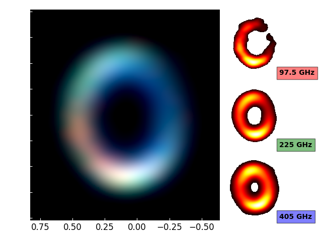
Figure 2: RGB image of the multi-frequency observations of ISO-Oph 2 A. Each image is masked below 10$\sigma$. Red: B3 continuum, restored with $r=0.7$, with a beam of $0\aas@@fstack{\prime\prime}230\times 0\aas@@fstack{\prime\prime}171$ along 90 deg. Green: B6 continuum, degraded to the B3 beam. Blue: B8 continuum, degraded to the B3 beam.

Figure 3: Intensity spectral index maps. a) Spectral index between B3 and B6, at the resolution of B3 ($r=0.7$). b) Spectral index between B6 and B8, at the resolution of B8 ($r=0$).

2.3 Astrometry of ISO-Oph 2B

The accuracy of the multi-frequency alignment is $\lesssim 9$ mas, which is slightly better than the rule-of-thumb for the ALMA pointing accuracy, of about $1/10$ of the clean beam (Remijan et al., 2019). In Table 2 we record the positions of ISO-Oph 2B, measured with elliptical Gaussian fits. The error budget is dominated by that of the Gaussian centroid, except for B6, for which we assign the nominal ALMA pointing accuracy.

It appears that ISO-Oph 2B is moving too fast, relative to ISO-Oph 2A, for Keplerian rotation. At their projected separation, of $\sim 257\,$au, the Keplerian velocity for a $0.5\,M_{\odot}$ system is $\sim$1.3 km s^-1, and only $\sim$0.8 km s^-1 after projection onto the plane of the sky with a disk inclination of 36 deg. However, the projected velocity comparing SB17 and B8 is $10.1\pm 3.4$ km s^-1, and is $6.0\pm 2.5$ km s^-1 when comparing B6 and B8. The difference with a bound orbit and circular orbit in the plane of the circum-primary disk are $\sim 2.7\sigma$ and $\sim$2.1$\sigma$. A new epoch is required to conclude.

To further assess the possibility of an unbound trajectory for ISO-Oph 2B, we attempted to fit the 5 astrometric measurements with a bound orbit using Orbitize! (Blunt et al., 2020). We assumed a total mass of $0.58\pm 0.15M_{\odot}$ for the system (0.5 $M_{\odot}$ for A and 80 $M_{J}$ for B; González-Ruilova et al., 2020), and a parallax of $7.449\pm 0.074$ mas (Gaia Collaboration et al., 2016, 2022). We considered two cases: no prior on the orbit, and tight Gaussian priors on the inclination and longitude of the ascending node for the orbital plane to match the plane of the circumprimary disc. In either cases, we drew 10,000 orbits with the OFTI algorithm and noted that the first epoch datum was $\sim$2 $\sigma$ diskrepant from the closest orbit predictions at that epoch out of these 2 $\times$ 10,000 samples. This provides another piece of evidence in favour of an unbound hyperbolic trajectory (i.e. a fly-by).

Table 2: Multi-epoch astrometry for ISO-Oph 2B, relative to the phase-center for B6. In this system, the GAIA coordinates for the primary are $\Delta\alpha=0\aas@@fstack{\prime\prime}101$, $\Delta\delta=0\aas@@fstack{\prime\prime}438$.

Date	Dataset	$\Delta\alpha^{a}$	$\Delta\delta^{b}$
2017-07-13	SB17	$0\aas@@fstack{\prime\prime}363\pm 0\aas@@fstack{\prime\prime}023$	$-1\aas@@fstack{\prime\prime}349\pm 0\aas@@fstack{\prime\prime}023$
2019-06-12	B6	$0\aas@@fstack{\prime\prime}399\pm 0\aas@@fstack{\prime\prime}003$	$-1\aas@@fstack{\prime\prime}385\pm 0\aas@@fstack{\prime\prime}003$
2021-07-27	B3	$0\aas@@fstack{\prime\prime}367\pm 0\aas@@fstack{\prime\prime}028$	$-1\aas@@fstack{\prime\prime}341\pm 0\aas@@fstack{\prime\prime}028$
2022-07-20	B4	$0\aas@@fstack{\prime\prime}423\pm 0\aas@@fstack{\prime\prime}024$	$-1\aas@@fstack{\prime\prime}368\pm 0\aas@@fstack{\prime\prime}024$
2022-08-04	B8	$0\aas@@fstack{\prime\prime}426\pm 0\aas@@fstack{\prime\prime}013$	$-1\aas@@fstack{\prime\prime}393\pm 0\aas@@fstack{\prime\prime}013$

^a Offset along R.A., in arcsec. ^b Offset along Dec., in arcsec.

2.4 Photometry

Table 3 reports the integrated flux densities for each component of ISO-Oph 2. For ISO-Oph 2A we used aperture photometry within a radius of $0\aas@@fstack{\prime\prime}8$, centered on the primary. For ISO-Oph 2B we used the integrated flux density obtained with elliptical Gaussian fits.

Table 3: Photometry of ISO-Oph 2 for each of the datasets presented in Fig. 1. We report flux densities in mJy. The errors do not include the systematic calibration uncertainty.

	B3	B4	B6	B8
ISO-Oph 2B	$0.32\pm 0.03$	$0.50\pm 0.07$	$1.81\pm 0.01$	$7.3\pm 0.3$
ISO-Oph 2A	$6.05\pm 0.15$	$23.6\pm 0.3$	$85.5\pm 0.5$	$316\pm 2$

2.5 Disk orientation and stellar offset

The position of ISO-Oph 2A (from GAIA DR 3, Gaia Collaboration, 2020), corrected for proper motion, is at $\Delta\alpha=0\aas@@fstack{\prime\prime}101$ and $\Delta\delta=0\aas@@fstack{\prime\prime}438$ relative to the B6-LB19 phase center. The errors on these coordinates are negligible relative to the ALMA pointing accuracy for B6-LB19, which is $\sim$3 mas. ISO-Oph 2A is remarkably offset from the ring centroid. Fig. 1 indicates the stellar position and the cavity centers for B6 and B8. We first centered each image on the primary, and then estimated the disk orientation and center using the MPolarMaps package (described in Casassus et al., 2021). MPolarMaps minimizes the azimuthal scatter in radial profiles, which should yield the correct orientation parameters for an axially symmetric disk. Under this assumption, the best fit parameters for B6 are a position angle PA$=2.42^{+0.45}_{-0.49}$ deg, an inclination of $i=36.92^{+0.21}_{-0.24}$ deg, and disk center relative to the stellar position: $\Delta\alpha=-0\aas@@fstack{\prime\prime}011\pm 0\aas@@fstack{\prime\prime}001$ $\Delta\delta=-0\aas@@fstack{\prime\prime}062\pm 0\aas@@fstack{\prime\prime}001$. The corresponding PA and $i$ are consistent with those reported by González-Ruilova et al. (2020). For B4, we obtain PA$=12.4^{+1.4}_{-1.4}$ deg, $i=31.8^{+0.8}_{-0.9}$ deg, and $\Delta\alpha=-0\aas@@fstack{\prime\prime}015\pm 0\aas@@fstack{\prime\prime}002$ $\Delta\delta=-0\aas@@fstack{\prime\prime}065\pm 0\aas@@fstack{\prime\prime}002$, while for B8, PA$=7.8^{+0.58}_{-0.65}$ deg, an inclination of $i=36.62^{+0.41}_{-0.38}$ deg, and disk center relative to the stellar position: $\Delta\alpha=-0\aas@@fstack{\prime\prime}001\pm 0\aas@@fstack{\prime\prime}001$ $\Delta\delta=-0\aas@@fstack{\prime\prime}076\pm 0\aas@@fstack{\prime\prime}001$.

In terms of their posterior distributions, the disk orientations inferred from MpolarMaps are well constrained (see Fig. 4). However, the above errors do not consider the systematics induced by the non-axial symmetry of the disk, which could well be intrinsically eccentric, hence the significant differences for each image. Still, a qualitatively large stellar offset, which can readily be seen by eye, is common to all 3 images. Such a large offset, of $\sim 62$ to $\sim 76$ mas, is rare in ringed systems with accurate optical/IR stellar astrometry. The associated eccentricity, for a 0$\aas@@fstack{\prime\prime}$43 ring, ranges between 0.12 and 0.17. By comparison, the largest of such offsets, inferred from long-baseline continuum ALMA data, is $33\pm 3$ mas in MWC 758 (Dong et al., 2018), and $12\pm 4$ mas in HD 135344B (Casassus et al., 2021). The ring around IRS 48 also appears to be extremely eccentric, with $e\sim 0.27$ and an offset between the ring centroid and the central sub-mm emission of $\sim$0$\aas@@fstack{\prime\prime}$15 (Yang et al., 2023).

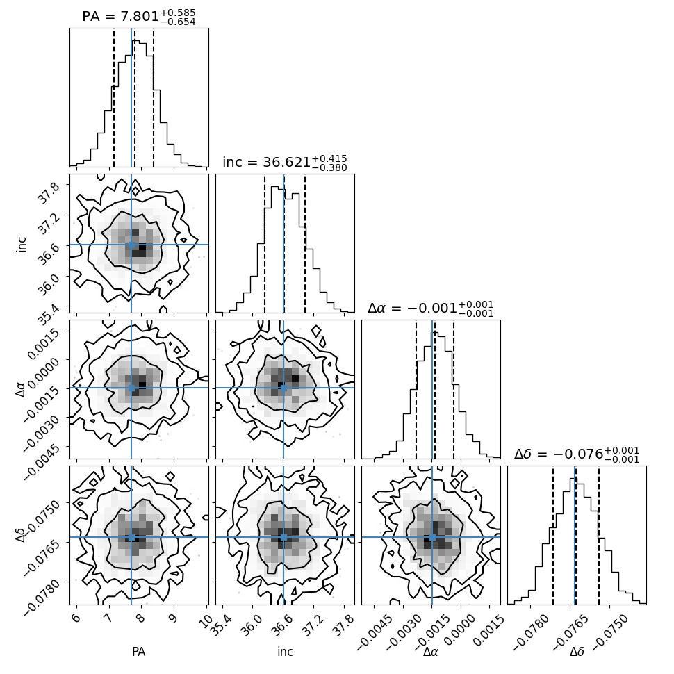
Figure 4: Corner plot from the optimisation of the orientation parameters in ISO-Oph 2 A, using the B8 image with $r=0$. The histograms plot the 1D probability density functions of the parameters indicated in titles, along with their median values and 1$\sigma$ confidence intervals (i.e. at 16% and 84%), which are also shown by the vertical dashed lines. The contour plots show the marginalized 2D distributions (i.e. the 2D projection of the 8D posterior probability distribution), for the corresponding pairs of parameters. Contour levels are chosen at 0.68, 0.95 and 0.997.

3 Analysis

3.1 Qualitative spectral trends

The RGB image in Fig. 2 is rich in structure, suggesting strong azimuthal variations in physical conditions. The low frequency spectral index $\alpha_{97.5}^{225}$ in Fig. 3a reveals a clump of values around $\sim 2.4$ to the South-East, which could be the result of optically thin emission from a concentration of large grains, while the rest of the disk corresponds to smaller grains with $\alpha_{97.5}^{225}\sim 3.0$. In turn $\alpha_{225}^{405}$ in Fig. 3b is more uniform with values of around 2.0 to the East, which could correspond to optically thick emission, while emission on the Western side is more optically thin, with $\alpha_{225}^{405}\sim 3$. An optically thick region to the East could correspond to a lopsided disk, which would be consistent with the large grain clump in the dust trap hypothesis: grains with larger dimensionless stopping time (Stokes number), up to $S_{t}\lesssim 1$, pile up near the center of the pressure maximum (e.g. Birnstiel et al., 2013; Lyra & Lin, 2013; Zhu & Stone, 2014; Mittal & Chiang, 2015; Baruteau & Zhu, 2016; Casassus et al., 2019a).

3.2 Implementation of uniform-slab diagnostics in Slab.Continuum

We quantify the dust trapping scenario by interpreting the spectral variations in terms of dust properties averaged along the line of sight. We developed the package Slab.Continuum to model the emergent intensities from a uniform-slab, including isotropic scattering (in the Eddington approximation and with two-streams boundary conditions, following Miyake & Nakagawa, 1993; D’Alessio et al., 2001; Sierra et al., 2017, 2019; Casassus et al., 2019a):

$$I^{m}_{\nu}(\tau_{\nu},\mu)=B_{\nu}(T)\left[1-\exp\left(-\frac{\tau_{\nu}}{\mu}\right)+\omega_{\nu}\mathcal{F_{\nu}}\right]$$ (1)

where

$$\begin{split}\mathcal{F_{\nu}}=&\frac{1}{(\sqrt{1-\omega_{\nu}}-1)\exp\left(-\sqrt{3(1-\omega_{\nu})}\tau_{\nu}\right)-(\sqrt{1-\omega_{\nu}}+1)}\times\\ &\left\{\frac{1-\exp\left[-\left(\sqrt{3(1-\omega_{\nu})}+\mu^{-1}\right)\tau_{\nu}\right]}{\sqrt{3(1-\omega_{\nu})}\mu+1}~{}+\right.\\ &\left.\frac{\exp\left(-\frac{\tau_{\nu}}{\mu}\right)-\exp\left(-\sqrt{3(1-\omega_{\nu})}\tau_{\nu}\right)}{\sqrt{3(1-\omega_{\nu})}\mu-1}\right\},\end{split}$$ (2)

$\omega=\frac{\kappa^{\rm sca}}{\kappa^{\rm abs}+\kappa^{\rm sca}}$ is the dust albedo, $\tau_{\nu}\equiv\Sigma_{g}\kappa_{\nu}$, and $\kappa_{\nu}=\kappa^{\rm abs}+\kappa^{\rm sca}$. The angle of incidence, $\mu=\cos(i)$, was set to 1 for simplicity, thus reducing Eq. 2 to Eqs. 24 and 25 of Sierra et al. (2019).

The size-averaged dust opacities $\kappa_{\nu}^{\rm abs}$ and $\kappa_{\nu}^{\rm sca}$ were computed using routines from the dsharp_opac package, described in Birnstiel et al. (2018), and with their default effective optical constants (Fig. 2 in Birnstiel et al., 2018, , i.e. “DSHARP” opacities). Forward scattering was accounted for by correcting the scattering opacity $\kappa_{\nu}^{\rm sca}$ to $(1-g_{\nu})\kappa_{\nu}^{\rm sca}$, where $g_{\nu}$ is the Henyey-Greenstein anisotropy parameter.

For a power-law distribution of dust grain sizes, with a single dust composition, and for a fixed gas-to-dust mass ratio (taken here to be 100), the free-parameters for any given line-of-sight are the total mass column density $\Sigma_{g}$, the maximum grain size $a_{\rm max}$, the dust size exponent $q$, and the dust temperature $T_{\rm d}$. We fit the spectral-energy-distribution (SED) for each line-of-sight, with $N$ independent frequency points $\{I_{\nu_{i}}\}_{i=1}^{N}$, by minimizing

$$\chi^{2}=\sum_{i}\frac{(I_{\nu_{i}}-I^{m}_{\nu_{i}})^{2}}{\sigma_{i}^{2}},$$ (3)

Where the weights $\{1/\sigma_{i}^{2}\}$ are approximated as the root-mean-square dispersion for each residual image, including the flux calibration error in quadrature. The flux calibration accuracy was taken to be 5% in B3, 5% in B4, 5% in B6, and 10% in B8.

The posterior disributions were calculated with a Markov chain Monte Carlo ensemble sampler (Goodman & Weare, 2010). We used the emcee package (Foreman-Mackey et al., 2013), with 1000 iterations, a burn-in of 800, and 10 walkers per free-parameter. Except for $q$, we varied the logarithm of each parameter, with flat priors, and across wide domains in parameter space: $0<\log(T_{\rm d}/{\rm K})<3$, $-5<\log(\left(\Sigma_{g}/{\rm g\,cm}^{-2}\right)<3$ and $-3<\log\left(a_{\rm max}/{\rm cm}\right)<10$, and $-3.99<q<-2$. The Slab.Continuum package optionally runs a final optimization with the Powell variant of the conjugate-gradient minimization algorithm, using the maximum likelihood parameters obtained with emcee. Rather than calculate size-averaged opacities for all sampled values of $a_{\rm max}$ and $q$, we first computed opacity grids in $a_{\rm max}$ and $q$, at each of the frequencies $\{\nu_{i}\}_{i=1}^{N}$, and used bi-linear interpolation.

3.3 Application of Slab.Continuum to ISO-Oph 2A

Initial trials including B4 resulted in strong biases due to beam dilution, when the beam is much larger than the structures (see below). We therefore discarded B4 from the spectral fits. With $N=3$ independent spectral points we may optimize only up to 3 parameters. For the present application of Slab.Continuum we thus chose to fix $q=-3.5$, i.e. as in the standard ISM size distribution (Mathis et al., 1977).

Before running the optimization on all lines-of-sights, and in order to reduce the load on computer resources, we resampled each image $\{I_{\nu_{i}}\}_{i=1}^{N}$ into coarser pixels (in synthesis imaging the pixel size is usually chosen to be around 1/10 of the natural-weights clean beam). We additionally set an intensity mask at $10\sigma$ in B6.

The coarsest data-point is B3, and thus the full set of frequency points was degraded to the B3 beam with $r=0$. The result is summarised in Fig. 5, where we see that the inferred dust parameters bear fairly large uncertainties, especially to the West, where the disk is faintest in B3. Example SEDs, for the lines-of-sight towards the intensity extrema in B6 and along the eastern side of the ring, are shown in Fig. 6. A corner-plot for the posterior probability distributions towards the peak is shown in Fig. 7. We see that $a_{\rm max}$ is poorly constrained, which we tentatively interpret in terms of two dominant effects. First, towards the minimum in B4, to the West of the ring, the solutions for large grains, $\log(a_{\rm max}/{\rm cm})>0.8$, correspond to optically thin emission at all frequencies, where intensities are proportional to optical depth, $I_{\nu}\propto T_{\rm d}\tau_{\nu}$. Since $\tau_{\nu}\propto\Sigma_{g}$, the lack of an additional point in the optically thick regime prevents lifting the $T_{\rm d}-\Sigma_{g}$ degeneracy. Second, even with an optically thick point with which to set $T_{\rm d}$, for grains that are larger than the wavelength, increasing grains larger have lower opacity $\kappa_{\nu}$, so that a given optical depth may result from arbitrarily large grains $\tau_{\nu}=\kappa_{\nu}\,\Sigma_{g}$, leading to the $a_{\rm max}-\Sigma_{g}$ degeneracy (e.g. Sierra et al., 2021). We set the maximum grain size to 100 cm, which corresponds to the maximum size in the default opacities from Birnstiel et al. (2018).

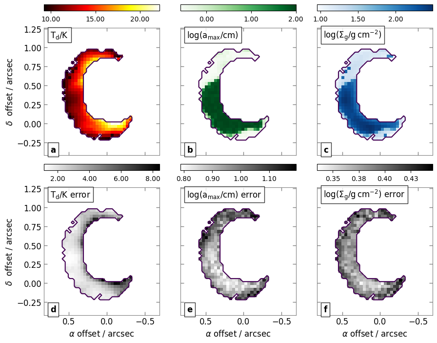
Figure 5: Dust parameters for each line of sight from the uniform-slab optimizations of $T_{\rm d}$, $a_{\rm max}$ and $\Sigma_{g}$, and constrained with the B3, B6 and B8 all degraded to the B3 beam with $r=0.7$. The black contours outline an error mask on $\log_{10}(T_{\rm d})$, set to 0.2. a: Maximum-likelihood $T_{\rm d}$. b: Maximum-likelihood $\log_{10}(a_{\rm max})$. c: Maximum-likelihood $\log_{10}(\Sigma_{g})$. d: One-sigma uncertainty on $T_{\rm d}$, approximated as $\sigma(T_{\rm d})=\ln(10)T_{\rm d}\sigma(\log(T_{\rm d}))$, where $\sigma(\log(T_{\rm d}))$ is estimated with the average of the upwards and downwards 34% confidence intervals around the median. e: One-sigma uncertainty on $\log_{10}(a_{\rm max})$. f: One-sigma uncertainty on $\log_{10}(\Sigma_{g})$. The blue lines correspond to the maximum-likelihood values.

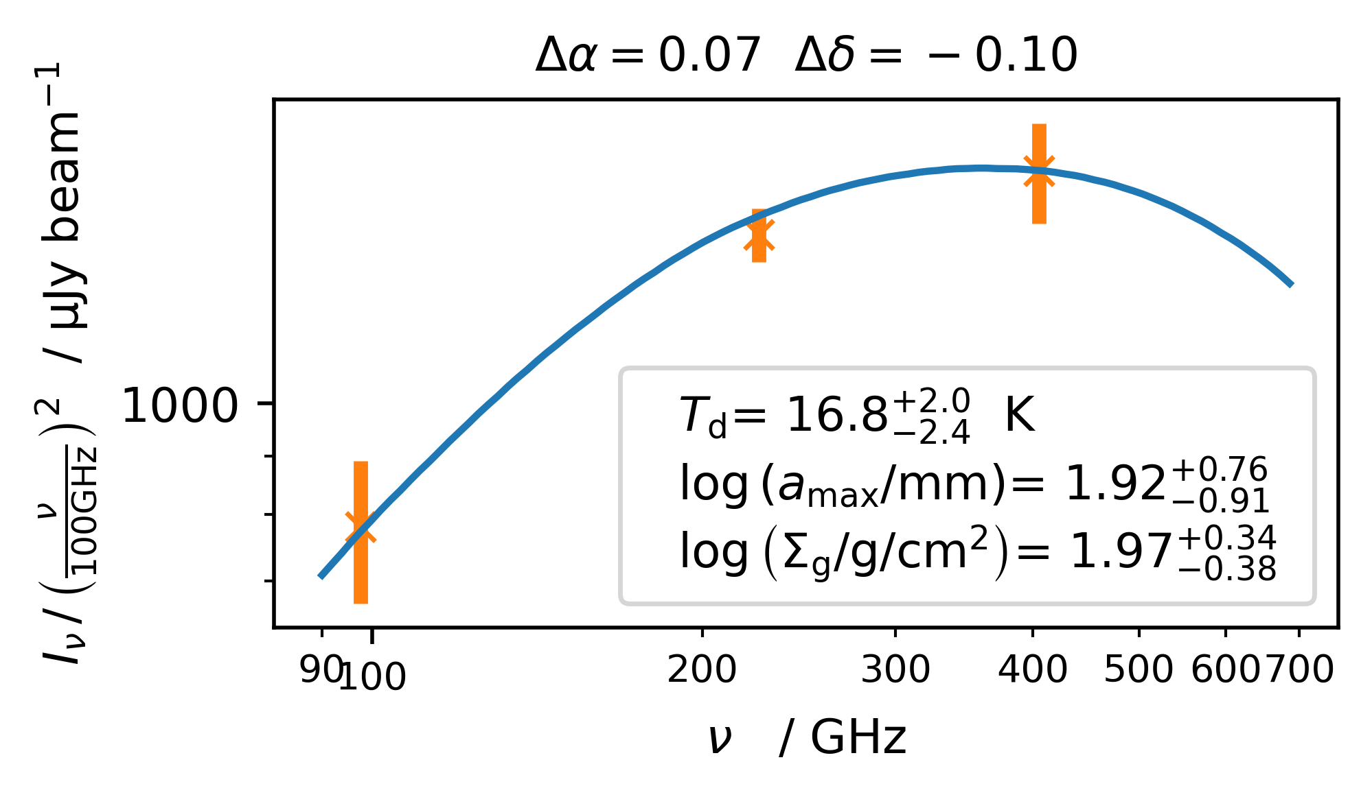
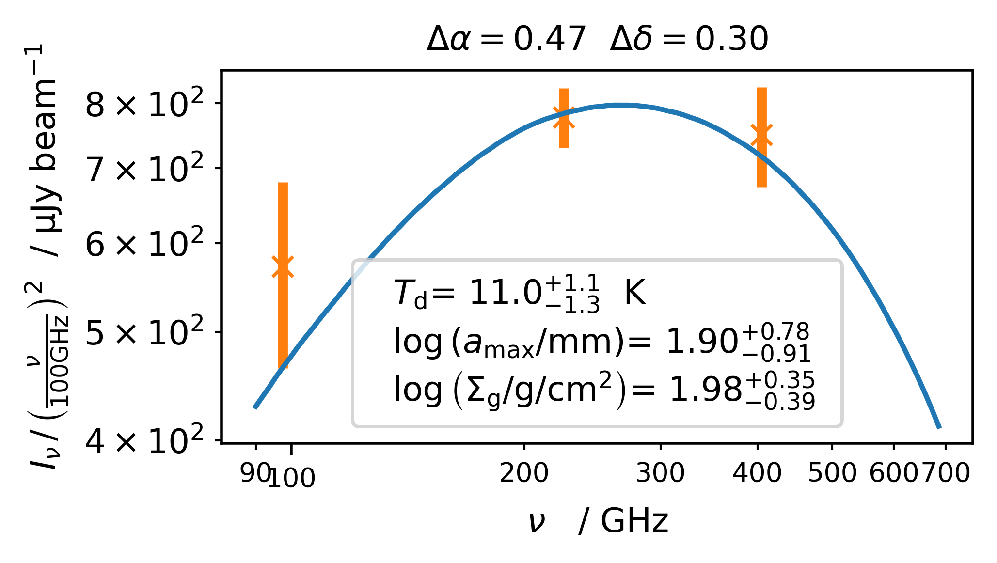
Figure 6: Spectral energy distribution and best-fit uniform-slab model for two example lines of sight (LOS). The direction of each LOS is given as offset from the phase centers, in arcsec, on top of each plot. Top: LOS towards the peak B6 intensity. Bottom: LOS towards the minimum in B6 intensity along the eastern side of the ring.

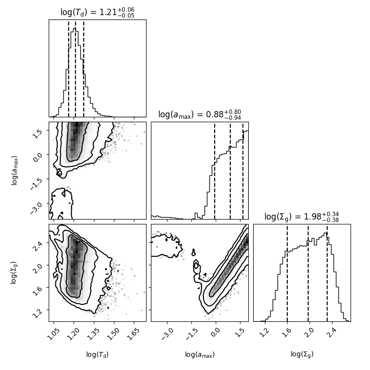
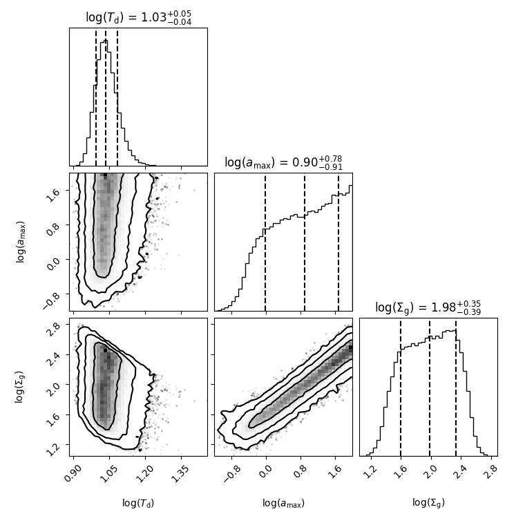
Figure 7: Annotations follow from Fig. 4. Left: Corner plot for the dust parameters towards the peak B6 intensity, corresponding to Fig. 6 (top). Left: Corner plot for the dust parameters towards the minimum B6 intensity along the Eastern ring, and corresponding to Fig. 6 (bottom).

3.4 Incorporation of a beam filling-factor

Beam-dilution, or the reduction of specific intensities in sources that do not fill the clean beam, is strong in the coarse B3 beam, even with $r=0$. This also translates into a reduction in brightness temperature, which reach only $\sim$5 K in B3, and $\sim$10 K in the finer beam of B6 (in ISO-Oph 2A, Fig. B). Without a beam filling factor among the free-parameters, the uniform-slab model is a poor approximation. For instance, in the case of $T_{\rm d}$ and optically thick emission, beam-dilution would lower the brightness temperature, but the spectral indices would still correspond to the undiluted black-body emission. Similarly, $a_{\rm max}$ determines the spectral indices and opacity, which may not match the observed intensities if they are diluted. A question arises on the impact of beam-dilution on the inferred physical parameters.

The B6 dataset is well-sampled, and can be used to estimate the filling factor in B6, by comparing the B6 map in native resolution ($I_{\rm B6}$) with its smoothed version ($I_{\rm B6}^{\rm s}$), $f=I_{\rm B6}^{\rm s}/I_{\rm B6}$, with an upper limit of 1. The resulting map is shown in Fig. 8. We use this map to scale the multi-frequency intensities, i.e. the corrected intensities are $I_{\nu}^{c}=I_{\nu}/f$. The corresponding dust properties are shown in Fig. 9 , with examples SEDs in Fig. 10. It is interesting to note that $\chi^{2}$, as given by Eq. 5, is reduced from 1.1 to 0.11 with the incorporation of the filling factor for the line of sight toward the peak B6 intensity. This probably reflects the improved model in B6. However, there is no appreciable difference for the line of sight towards the minimum B6 intensity (to the East of the ring), where $\chi^{2}$ increases from 1.1 to 1.2 with the inclusion of a filling factor.

Figure 8: Beam filling factor inferred from the B6 dataset.

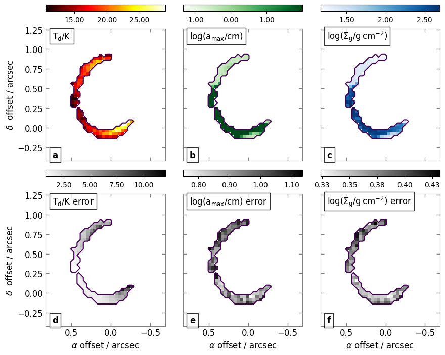
Figure 9: Dust parameters for each line of sight from the uniform-slab optimizations of $T_{\rm d}$, $a_{\rm max}$ and $\Sigma_{g}$, including a filling-factor, and constrained with the B3, B6 and B8 all degraded to the B3 beam with $r=0.7$. Annotations follow from Fig. 5.

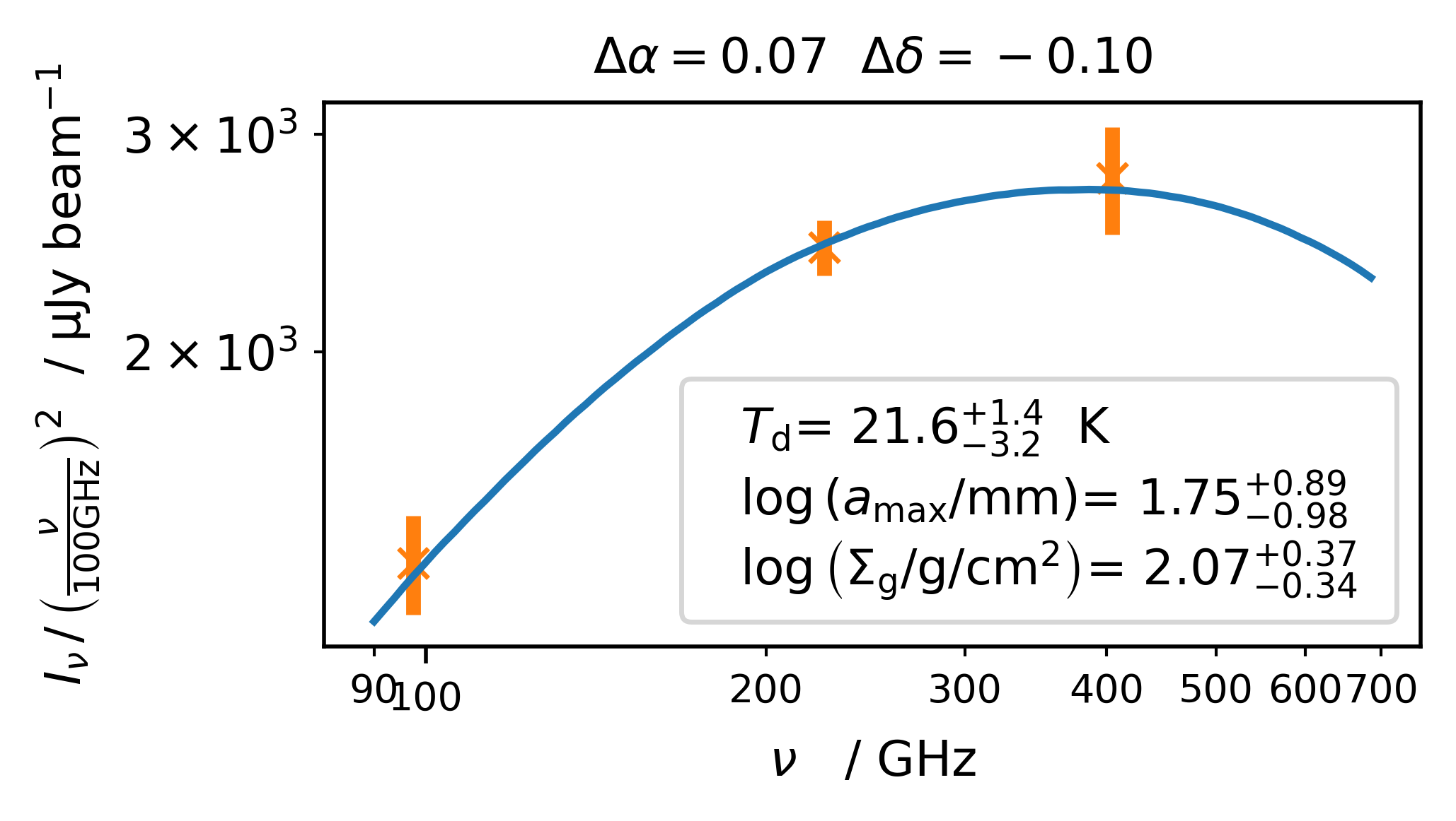
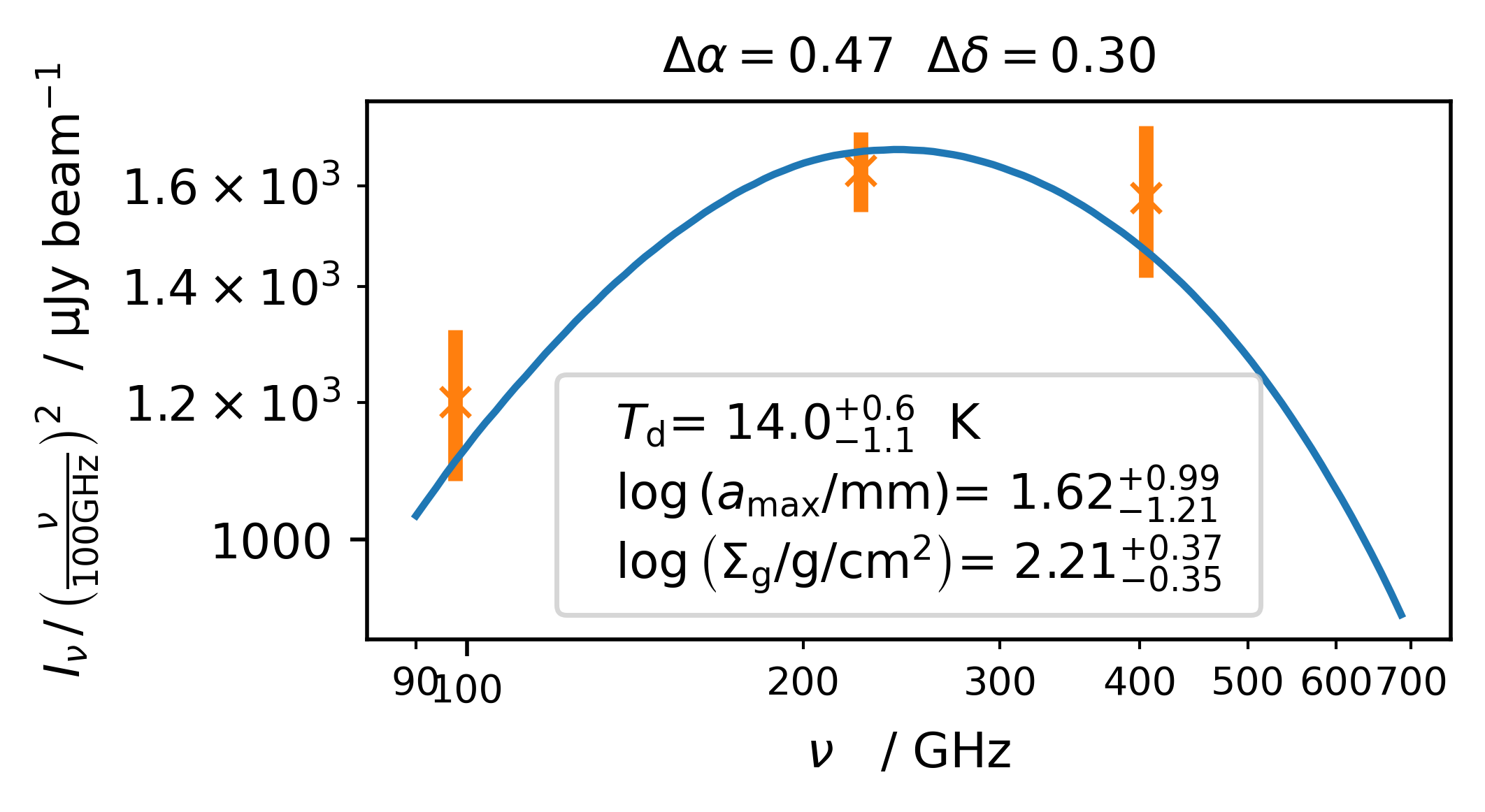
Figure 10: Spectral energy distribution and best-fit uniform-slab model for two example lines of sight (LOS), with a filling factor. Annotations follow from Fig. 6.

3.5 Fixing $a_{\rm max}$

In Fig. 11 we explore a fit with only two free-parameters, i.e. $T_{\rm d}$ and $\Sigma_{g}$. In order to reach the optically thick limit close to B8, and thus lift the $T_{\rm d}-\Sigma_{g}$ degeneracy, we set $a_{\rm max}=0.01\,$cm. This choice yields well-constrained posteriors for $T_{\rm d}$ and $\Sigma_{g}$. Fixing $a_{\rm max}\gtrsim 1\,$cm results in optically thin emission to the West, and large errors on $T_{\rm d}$. However, in the East the morphologies of $T_{\rm d}$ and $\Sigma_{g}$ are very similar in both cases.

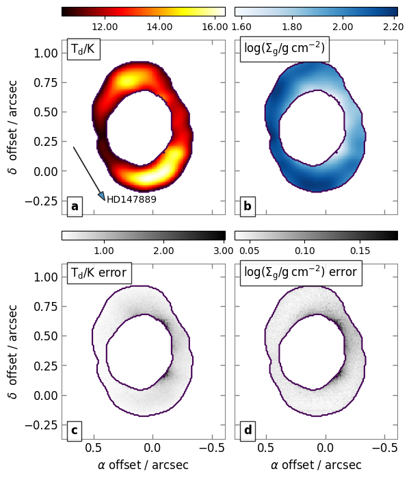
Figure 11: Dust parameters for each line of sight from the uniform-slab optimizations of $T_{\rm d}$ and $\Sigma_{g}$, constrained with the B8 and B6 data, degraded to the B8 beam with $r=0$. The black contours outline an intensity mask, set to $20\,\sigma$ in B8. a: Maximum-likelihood $T_{\rm d}$. The arrow points to the direction of HD 147889. b: Maximum-likelihood $\log_{10}(\Sigma_{g})$. c: One-sigma uncertainty on $T_{\rm d})$, approximated as $\sigma(T_{\rm d})=\ln(10)T_{\rm d}\sigma(\log(T_{\rm d}))$. d: One-sigma uncertainty on $\log_{10}(\Sigma_{g})$.

3.6 Discussion

An interesting result of the present estimates of physical conditions are the significant variations in $T_{\rm d}$ along the ring, and especially along the eastern arc. In the fits including B3, the minimum along the ring is $\log(T_{\rm d}/K)=1.04\pm 0.04$, while $T_{\rm d}$ reaches $\log(T_{\rm d}/K)=1.32\pm 0.08$ to the North and South. The fits to the B6 and B8 data reach higher $T_{\rm d}$, as expected since beam-dilution is reduced, and cover all azimuth. In Fig. 12 we extracted the azimuthal profile for $T_{\rm d}$, for which we adopted the orientation from the B8 estimates, i.e. PA=7.8 deg and $i=36.6$ deg. The variations in $T_{\rm d}$ are quite significant, and reach $\log(T_{\rm d}/K)=1.175\pm 0.017$ in the North, and $\log(T_{\rm d}/K)=1.210\pm 0.015$ in the South, with a minimum towards the East at $\log(T_{\rm d}/K)=1.036\pm 0.014$, which represents over $8\sigma$.

Interestingly, the PA on the sky of the line joining the two peaks in Fig. 12b is 193.5 deg, and is remarkably close to the direction of HD 147889, which is at 210.5 deg. The azimuthal temperature modulation might thus result from a variation of the angle of incidence of radiation coming from HD 147889. Such external irradiation would hit the Southern edge of the disk almost edge-on, and, since the disk is flared, the region where it would reach the disk surface at closest to normal incidence is to the North. The small difference between the PA joining the two temperature maxima might be due to biases in our estimate of the dust temperature, since here we kept the dust grain size fixed at a small value that ensures that B8 is in the optically thick regime. Another interesting possibility is that, if the disk is retrograde (rotating clock-wise), then the small angular shift could be due to the thermal lag discussed in Casassus et al. (2019b).

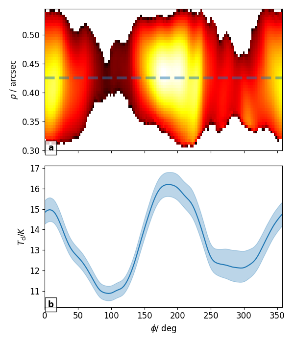
Figure 12: Polar expansion of the temperature map from Fig. 11a, shown with the same colour scale, and its azimuthal profile, as extracted at a radius $\rho=0\aas@@fstack{\prime\prime}425$. The shaded area corresponds to the region enclosed by the 1-$\sigma$ uncertainties (its total vertical extent is 2$\sigma$). The extraction radius is indicated as a dashed line in $a)$.

4 Conclusions

We report new ALMA continuum observations of the ISO-Oph 2 binary, at 97 GHz, 145 GHz and 405 GHz, that complement existing 225 GHz data. A novel strategy for the alignment of multi-frequency data, acquired with broadly different angular resolutions, allowed us to reach the following conclusions:

1. The offset of ISO-Oph 2A relative to the centroid of the circumprimary disk is remarkably large, of 62 mas to 76 mas depending on the image (Fig. 1). Such a large offset points at dynamical interactions, either with ISO-Oph 2B or with other massive bodies inside the ring of ISO-Oph 2A.

2. The multi-frequency data reveal strong morphological variations with frequency in ISO-Oph 2A (Fig. 2). We linked these variations to the underlying physical conditions by modeling the data with uniform-slab intensities (Figs. 5 and 11).

3. Surprisingly, the dust temperature varies strongly in azimuth (Fig. 12), and roughly traces a second harmonic with 4 nodes. The PA joining the two peaks, each to the North and South of the disk, is aligned in the direction towards HD 147889 within 10 deg. Such an azimuthal temperature modulation is in qualitative agreement with external irradiation as the dominant heat source.

4. As in several other disks, we find indications for a lopsided disk, where the dust column density is shaped into a crescent. The maximum grain size appears to coincide with the peak column density, as expected for aerodynamic dust trapping (Fig. 5).

5. The multi-epoch astrometry of the binary is only marginally consistent with a bound orbit, in support (but at $\sim 2\sigma$) of the view that the binary is in fact a fly-by.

The binary disks of ISO-Oph 2 are interesting laboratories for the impact of environmental effects on disk structure, with strong dynamical perturbations on the circumprimary ring. The temperature structure of this ring is also suggestive of heating by external irradiation, probably from HD 147889. This possibility will be considered in a companion article on radiative transfer modeling of external irradiation in ISO-Oph 2.

Data Availability

The reduced ALMA data presented in this article are available upon reasonable request to the corresponding author. The original or else non-standard software packages underlying the analysis are available at the following URLs: MPolarMaps (https://github.com/simoncasassus/MPolarMaps, Casassus et al., 2021), uvmem (https://github.com/miguelcarcamov/gpuvmem, Cárcamo et al., 2018), pyralysis (https://gitlab.com/clirai/pyralysis), VisAlign (https://github.com/simoncasassus/VisAlign), snow (https://github.com/miguelcarcamov/snow).

Appendix A On the JvM correction

The so-called “JvM correction” (Jorsater & van Moorsel, 1995; Czekala et al., 2021) is thought to improve the dynamic range of images restored from radio-interferometric data. However, here we did not apply the JvM correction, because the resulting improvement is due to a spurious down-scaling of the image residuals, as shown in Casassus & Cárcamo (2022). Despite the proof, since its publication several workers have kept on applying the JvM correction, which leads us to believe that perhaps the arguments presented in Casassus & Cárcamo (2022) may not be clear enough. Here we give more details on the argumentation that defines the units of the dirty map in interferometric image reconstruction.

As summarised in Appendix A of Casassus & Cárcamo (2022, Eq. A2 ), the restored image is obtained by adding the dirty map $R_{D}$ of the visibility residuals with the model image $I_{m}$, after convolution with the clean beam $g_{b}$:

$$I_{R}=I_{m}\ast g_{b}+R_{D}.$$ (4)

Both the convolved model image and dirty residuals must of course bear the same units. Casassus & Cárcamo (2022) proposed to tie these units to the case of a point source at the phase center, where the flux of the point source and its uncertainty can be inferred from parametric modelling of the visibility data (e.g. their Eqs. A11 and A12). They matched this uncertainty to the thermal uncertainty on the specific intensity in the dirty map at the phase center (their Eqs. A13 and A14).

However, Casassus & Cárcamo (2022) did not explain the relationship between the general expression for the dirty map $I_{D}$ (originally in Eq. A9) and that of the residuals $R_{D}$ in Eq. 4 above. Here we clarify that, for the test-case of a point source at the phase center, the uncertainties on $I_{R}$ stem from the thermal noise in $R_{D}$, since the model of the source is known. The dirty map $R_{D}$ is itself an application of the general formula for $I_{D}$ to the residual visibilities of the parametric fit. These residuals should contain only noise in this idealised test-case.

Appendix B Brightness temperature maps

Fig. 13 includes a summary of the self-calibrated and aligned data, as in Fig. 1, but in brightness temperature.

Figure 13: Same as Fig. 1, but for brightness temperature maps. The images have been clipped at 0 K.

Appendix C Figure of merit for the alignment of visibility datasets

The alignment of the multi-frequency visibility data was performed with the VisAlign package, described in Casassus & Cárcamo (2022). However, here we improved VisAlign with an adjustment to the figure of merit, as the least-squares formula associated to the alignment of two visibility datasets, i.e. Equation 1 in Casassus & Cárcamo (2022), was biased in the choice of reference dataset. In this appendix we revisit the least-squares figure of merit used to perform the alignment of two visibility datasets, i.e. Equation 1 in Casassus & Cárcamo (2022), which we reproduce here for clarity:

$$\chi^{2}_{\rm align}(\alpha_{R},\delta{\vec{x}})=\sum_{k=1}^{N}W^{\rm align}_{k}\|\tilde{V}_{k}^{L}-\tilde{V}_{k}^{Lm}\|^{2},$$ (5)

where

$$\tilde{V}_{k}^{Lm}=\alpha_{R}\,e^{i2\pi\,\delta\vec{x}\cdot\vec{u}_{k}}\,\tilde{V}_{k}^{S},$$ (6)

and

$$W_{k}^{\rm align}=\frac{W_{k}^{S}\,W_{k}^{L}}{W_{k}^{S}+W_{k}^{L}}.$$ (7)

With such weights $W_{k}$, the minimization of $\chi^{2}_{\rm align}$ in Eq. 5 is not symmetric in the choice of reference dataset for the alignment of the two visibilty datasets $\left\{\tilde{V}^{S}_{k}\right\}_{k=1}^{N}$ and $\left\{\tilde{V}^{L}_{k}\right\}_{k=1}^{N}$. In other words, aligning $\tilde{V}^{S}$ to $\tilde{V}^{L}$ does not yield the opposite shift and reciprocal flux correction as aligning $\tilde{V}^{L}$ to $\tilde{V}^{S}$. A symmetric expression, now implemented in the VisAlign package, is obtained by replacing the weights with:

$$W_{k}^{\rm align}=\frac{W_{k}^{S}\,W_{k}^{L}}{W_{k}^{S}+\alpha_{R}^{2}W_{k}^{L}}.$$ (8)

We confirmed that with this modification the alignment is now independent on the choice of reference data-set, in the sense that the astrometric shifts are opposite and the flux scale factors are reciprocal (down to the round-off numerical accuracy).

The impact on the corresponding flux scale factors and astrometric shifts is small ($\sim 5\%-10\%$). For example, following the nomenclature of Benisty et al. (2021) for the each visibility dataset, the updated flux scale correction factors are $\alpha_{R}=0.817\pm 0.003$ to match SB16 to LB19, and $\alpha_{R}=0.837\pm 0.002$ to match IB17 and LB19.

Another consequence is that the shifts are no longer sensitive on the choice of $uv-$range, and depend only on the choice of $uv$-plane cell size for gridding, $\Delta u$. We checked that the shifts are all consistent within the errors for widely different choices of $\Delta u$, ranging from the antenna diameter to the minimum baseline length.

Appendix D Update to the multi-epoch radio-continuum imaging of PDS 70

The impact of the revised alignment on the corresponding flux scale factors and astrometric shifts, although small ($\sim 5\%-10\%$), affects the multi-epoch analysis of PDS 70 reported in Casassus & Cárcamo (2022). Here we update the resulting images. All the conclusions from Casassus & Cárcamo (2022) hold, but the variability of PDS 70c is more significant.

As in Casassus & Cárcamo (2022), we self-calibrated each data-set individually before concatenation. Self-calibration was performed automatically with the OOselfcal package, which we re-baptised to “Self-calibratioN Object-oriented frameWork”, i.e. snow. A consequence of the updated figure of merit is that the peak signal-to-noise ratios for the concatenated datasets are already close to the values obtained after joint self-calibration.

The LB19 dataset was used as reference for the alignment of the multi-epoch data. However, the 2020 GAIA coordinates (DR 3, Gaia Collaboration, 2020) for PDS 70 are offset by 9.2 mas relative to the LB19 phase center, by 8.2 mas in R.A. and -4.2 mas in Dec.. This shift is larger than the nominal pointing accuracy of the LB19 dataset (whose standard deviation is about a tenth of a beam or $\sim$5 mas).

In addition to the correction on the alignment procedure, the scheduling block from Dec. 6, 2017, was missing in the images for the IB17 dataset re-processed in Casassus & Cárcamo (2022), who therefore included only 2/3 of the available dataset. The incorporation of this scheduling block improves the sensitivity of the IB17 images, and results in tighter constraints on the absence of PDS 70c in the IB17 data. The corrected images are shown in Fig. 14.

A final correction to the analysis presented in (Cárcamo et al., 2018) concerns the choice of reference frequency for multi-frequency synthesis. In the uvmem imaging package (Cárcamo et al., 2018), multi-frequency synthesis is implemented with two options. The user can select to fit a spectral index map $\alpha(\vec{x})$ to the data, or use a single and constant spectral index value $\alpha$ to propagate the model visibilities to all frequencies (in specific intensity units, i.e $I_{\nu}=I_{\circ}(\nu/\nu_{\circ})^{\alpha}$). We usually adopt a flat spectral index, $\alpha=0$, but Casassus & Cárcamo (2022) opted to fix $\alpha=3$, with a reference frequency taken as the median of the centroid frequencies of all spectral windows in the concatenated datasets. This choice of reference frequency is slightly different from the default in CASA tclean, which uses the middle frequency. We have now unified the choice of frequency, as required for image restoration. With this correction the point source in LB19 coincident with PDS 70c is now also visible in the concatenation LB19+IB17+SB16 (see Fig. 14c).

Figure 14: Annotations follow from Fig. 4 in Casassus & Cárcamo (2022), except for the red cross in the insets on the inner disk, which is now pointed at the latest GAIA coordinates for PDS 70. The updated beam and noise values follow. a: Clean beam $\Omega_{b}=0\aas@@fstack{\prime\prime}048\times 0\aas@@fstack{\prime\prime}040\,/\,61$ deg. The noise in the residual image is $\sigma=16.6\,\mu$Jy beam^-1. b: $\Omega_{b}=0\aas@@fstack{\prime\prime}047\times 0\aas@@fstack{\prime\prime}039\,/\,57$deg, $\sigma=15.5\,\mu$Jy beam^-1. c: $\Omega_{b}=0\aas@@fstack{\prime\prime}056\times 0\aas@@fstack{\prime\prime}047\,/\,67$deg, and $\sigma=13.1\,\mu$Jy beam^-1. d: $\Omega_{b}=0\aas@@fstack{\prime\prime}062\times 0\aas@@fstack{\prime\prime}046\,/\,60$ deg, and $\sigma=25.9\,\mu$Jy beam^-1. e: $\Omega_{b}=0\aas@@fstack{\prime\prime}066\times 0\aas@@fstack{\prime\prime}050\,/\,61$ deg, and $\sigma=23.8\,\mu$Jy beam^-1. f: approximate resolution of 1/3 the natural weight beam (Cárcamo et al., 2018), or $\Omega_{b}\approx 0\aas@@fstack{\prime\prime}033\times 0\aas@@fstack{\prime\prime}029\,/\,88$ deg. The contours start at 3 $\sigma$, where $\sigma=0.16\,\mu$Jy pix^-1 is a representative noise level (with 4 mas pixels).

The noise level in the residuals for the SB16+IB17 image is 23.9 $\mu$Jy beam^-1 (versus 31.9 $\mu$Jy beam^-1 in our original publication). The point source coincident with PDS 70c in the LB19 dataset, with peak flux 118.5 $\mu$Jy beam^-1 (from Fig. 14a), should have been picked up in IB17 at 5.0$\sigma$. The point source injections tests are accordingly updated in Fig. 15. With these new numbers, if we assign a 3$\sigma$ upper limit flux for PDS 70c in IB17, then it was fainter by $40\%\pm 8\%$ relative to LB19 (versus $42\%\pm 13\%$ in the original publication).

Figure 15: Annotations follow from Fig. 6 in Casassus & Cárcamo (2022).

An update on the face-on views of the inner disk, and its variability, is given in Fig. 16, including the updated stellar position. The relative pointing accuracy of the multi-epoch data, as estimated from VisAlign, is $\sim 0.4$ mas, but the absolute pointing accuracy of the LB19 data-set is $\sim$5 mas and affects both epochs equally (in the same direction). The accuracy on the position of the ring centroid is 0.5 mas in SB16+LB19 and 0.7 mas in SB16+IB17. The offset between the nominal stellar position and the ring centroid is 8 mas in IB17, and 10 mas in LB19.

Figure 16: Annotations follow from Fig. 7 in Casassus & Cárcamo (2022), except that the red plus sign is now centered on the ring centroid (at the origin of coordinates), while the orange star indicates the position of the star.

In summary, the improvements to the analysis of the multi-epoch radio-continuum data from PDS 70 lead to tigher constraints on the variability of PDS 70c. The associated point source is variable by at least 40$\pm$ 8% in 1.75 yr, assigning the upper limit flux of 3$\sigma$ in the 2017.

References

- Andrews et al. (2009) Andrews S. M., Wilner D. J., Hughes A. M., Qi C., Dullemond C. P., 2009, ApJ, 700, 1502
- Andrews et al. (2010) Andrews S. M., Wilner D. J., Hughes A. M., Qi C., Dullemond C. P., 2010, ApJ, 723, 1241
- Ansdell et al. (2016) Ansdell M., et al., 2016, ApJ, 828, 46
- Ansdell et al. (2018) Ansdell M., et al., 2018, ApJ, 859, 21
- Barenfeld et al. (2016) Barenfeld S. A., Carpenter J. M., Ricci L., Isella A., 2016, ApJ, 827, 142
- Baruteau & Zhu (2016) Baruteau C., Zhu Z., 2016, MNRAS, 458, 3927
- Benisty et al. (2021) Benisty M., et al., 2021, ApJ, 916, L2
- Birnstiel et al. (2013) Birnstiel T., Dullemond C. P., Pinilla P., 2013, A&A, 550, L8
- Birnstiel et al. (2018) Birnstiel T., et al., 2018, ApJ, 869, L45
- Blunt et al. (2020) Blunt S., et al., 2020, AJ, 159, 89
- Cárcamo et al. (2018) Cárcamo M., Román P. E., Casassus S., Moral V., Rannou F. R., 2018, Astronomy and Computing, 22, 16
- Casassus & Cárcamo (2022) Casassus S., Cárcamo M., 2022, MNRAS, 513, 5790
- Casassus et al. (2006) Casassus S., Cabrera G. F., Förster F., Pearson T. J., Readhead A. C. S., Dickinson C., 2006, ApJ, 639, 951
- Casassus et al. (2008) Casassus S., et al., 2008, MNRAS, 391, 1075
- Casassus et al. (2019a) Casassus S., et al., 2019a, MNRAS, 483, 3278
- Casassus et al. (2019b) Casassus S., Pérez S., Osses A., Marino S., 2019b, MNRAS, 486, L58
- Casassus et al. (2021) Casassus S., et al., 2021, MNRAS, 507, 3789
- Cieza et al. (2019) Cieza L. A., et al., 2019, MNRAS, 482, 698
- Cieza et al. (2021) Cieza L. A., et al., 2021, MNRAS, 501, 2934
- Cox et al. (2017) Cox E. G., et al., 2017, ApJ, 851, 83
- Cuello et al. (2023) Cuello N., Ménard F., Price D. J., 2023, European Physical Journal Plus, 138, 11
- Czekala et al. (2021) Czekala I., et al., 2021, ApJS, 257, 2
- D’Alessio et al. (2001) D’Alessio P., Calvet N., Hartmann L., 2001, ApJ, 553, 321
- Dong et al. (2018) Dong R., et al., 2018, ApJ, 860, 124
- Dong et al. (2022) Dong R., et al., 2022, Nature Astronomy, 6, 331
- Eisner et al. (2018) Eisner J. A., et al., 2018, ApJ, 860, 77
- Foreman-Mackey et al. (2013) Foreman-Mackey D., Hogg D. W., Lang D., Goodman J., 2013, PASP, 125, 306
- Gaia Collaboration (2020) Gaia Collaboration 2020, VizieR Online Data Catalog, p. I/350
- Gaia Collaboration et al. (2016) Gaia Collaboration et al., 2016, A&A, 595, A1
- Gaia Collaboration et al. (2022) Gaia Collaboration et al., 2022, arXiv e-prints, p. arXiv:2208.00211
- González-Ruilova et al. (2020) González-Ruilova C., et al., 2020, ApJ, 902, L33
- Goodman & Weare (2010) Goodman J., Weare J., 2010, Communications in Applied Mathematics and Computational Science, Vol.~5, No.~1, p.~65-80, 2010, 5, 65
- Guilloteau et al. (2011) Guilloteau S., Dutrey A., Piétu V., Boehler Y., 2011, A&A, 529, A105
- Haworth (2021) Haworth T. J., 2021, MNRAS, 503, 4172
- Isella et al. (2009) Isella A., Carpenter J. M., Sargent A. I., 2009, ApJ, 701, 260
- Jorsater & van Moorsel (1995) Jorsater S., van Moorsel G. A., 1995, AJ, 110, 2037
- Long et al. (2018) Long F., et al., 2018, ApJ, 869, 17
- Long et al. (2019) Long F., et al., 2019, ApJ, 882, 49
- Longmore et al. (2021) Longmore S. N., Chevance M., Kruijssen J. M. D., 2021, ApJ, 911, L16
- Lyra & Lin (2013) Lyra W., Lin M.-K., 2013, ApJ, 775, 17
- Mann et al. (2014) Mann R. K., et al., 2014, ApJ, 784, 82
- Mathis et al. (1977) Mathis J. S., Rumpl W., Nordsieck K. H., 1977, ApJ, 217, 425
- Mittal & Chiang (2015) Mittal T., Chiang E., 2015, ApJ, 798, L25
- Miyake & Nakagawa (1993) Miyake K., Nakagawa Y., 1993, Icarus, 106, 20
- O’dell & Wen (1994) O’dell C. R., Wen Z., 1994, ApJ, 436, 194
- Pascucci et al. (2016) Pascucci I., et al., 2016, ApJ, 831, 125
- Remijan et al. (2019) Remijan A., et al., 2019, ALMA Technical Handbook,ALMA Doc. 7.3, ver. 1.1, 2019, doi:10.5281/zenodo.4511522
- Ruíz-Rodríguez et al. (2018) Ruíz-Rodríguez D., et al., 2018, MNRAS, 478, 3674
- Shuai et al. (2022) Shuai L., Ren B. B., Dong R., Zhou X., Pueyo L., De Rosa R. J., Fang T., Mawet D., 2022, ApJS, 263, 31
- Sierra et al. (2017) Sierra A., Lizano S., Barge P., 2017, ApJ, 850, 115
- Sierra et al. (2019) Sierra A., Lizano S., Macías E., Carrasco-González C., Osorio M., Flock M., 2019, ApJ, 876, 7
- Sierra et al. (2021) Sierra A., et al., 2021, ApJS, 257, 14
- Villenave et al. (2021) Villenave M., et al., 2021, A&A, 653, A46
- Wilhelm et al. (2023) Wilhelm M. J. C., Portegies Zwart S., Cournoyer-Cloutier C., Lewis S. C., Polak B., Tran A., Mac Low M.-M., 2023, MNRAS, 520, 5331
- Williams et al. (2019) Williams J. P., Cieza L., Hales A., Ansdell M., Ruiz-Rodriguez D., Casassus S., Perez S., Zurlo A., 2019, ApJ, 875, L9
- Winter & Haworth (2022) Winter A. J., Haworth T. J., 2022, European Physical Journal Plus, 137, 1132
- Winter et al. (2020) Winter A. J., Kruijssen J. M. D., Longmore S. N., Chevance M., 2020, Nature, 586, 528
- Yang et al. (2023) Yang H., Fernández-López M., Li Z.-Y., Stephens I. W., Looney L. W., Lin Z.-Y. D., Harrison R., 2023, ApJ, 948, L2
- Zhu & Stone (2014) Zhu Z., Stone J. M., 2014, ApJ, 795, 53
- Zurlo et al. (2020) Zurlo A., et al., 2020, MNRAS, 496, 5089
- Zurlo et al. (2021) Zurlo A., et al., 2021, MNRAS, 501, 2305