The torsion of stellar streams

Abstract

Context. Flat rotation curves $v(r)$ are naturally explained by elongated (prolate) Dark Matter (DM) distributions, and we have provided competitive fits to the SPARC database . To further probe the geometry of the halo, or the equivalent source of gravity in other formulations, one needs out-of-plane observables. Stellar streams, poetically analogous to airplane contrails, but caused by tidal dispersion of massive substructures such as satellite dwarf galaxies, would lie on a plane (consistently with angular momentum conservation) should the DM-halo gravitational field be spherically symmetric. Entire orbits are seldom available because their periods are commensurable with Hubble time, with streams often presenting themselves as short segments.

Aims. Therefore, we aim at establishing stellar stream torsion, a local observable that measures the deviation from planarity in differential curve geometry, as a diagnostic providing sensitivity to aspherical DM distributions which ensures the use of even relatively short streams.

Methods. We perform small-scale simulations of tidally distorted star clusters to check that indeed a central force center produces negligible torsion while distorted haloes can generate it. Turning to observational data, we identify among the known streams those that are at largest distance from the galactic center and likely not affected by the Magellanic clouds, as most promising for the study, and by means of polynomial fits we extract their differential torsion.

Results. We find that the torsion of the few known streams that should be sensitive to most of the Milky Way’s DM Halo is much larger than expected for a central spherical bulb alone. This is consistent with nonsphericity of the halo.

Conclusions. Future studies of stellar stream torsion with larger samples and further out of the galactic plane should be able to extract the ellipticity of the halo to see whether it is just a slight distortion of a spherical shape or rather ressembles a more elongated cigar.

1 Introduction: shape of Dark Matter Haloes

The problem of galactic rotation is the empirical statement that rotational velocity around the galactic center seems to flatten out for a large fraction of the galaxy population where this has been measured at long enough distances Rubin et al. (1978). This is at odds with orbital equilibrium outside a spherical source (Kepler’s third law written for the velocity),

$$\frac{v^{2}}{r}=\frac{GM}{r^{2}}\implies v=\sqrt{\frac{GM}{r}}$$ (1)

that implies falling velocities for objects or clouds of gas further away. Because typical velocities in spiral galaxies are of order 200-300 km/s, $v/c\sim 10^{-3}$, relativity is a correction and Newtonian mechanics should get the bulk of the rotation right. Therefore, either a modification of mechanics, such as MOND Milgrom (1983), or a modification of the gravity source, typically in the form of a spherical Dark Matter halo Frenk et al. (1985), are invoked. MOND however runs into problems at larger, cosmological scales Aguirre et al. (2001); Dodelson & Liguori (2006); and a spherical DM distribution has to be fine-tuned to have very nearly an isothermal $\rho(r)\propto 1/r^{2}$ profile to explain the flatness of the rotation curve.

If we inhabited a two-dimensional cosmos, however, the natural gravitational law would be $|F|\propto\frac{1}{r}$ instead of $\propto\frac{1}{r^{2}}$ and the observed rotational law would be $v_{\rm 2D}\propto{\rm constant}$ which is the law that the experimental data demands. We do not; but a cylindrical matter source achieves the same dimensional reduction by providing translational symmetry along the $OZ$ symmetry axis of the cylinder Slovick (2010); Llanes-Estrada (2021). If the linear density of the cylindrical dark matter source is $\lambda$, we can write

$$\frac{v^{2}}{r}=\frac{2G\lambda}{r}\implies v=\sqrt{2G\lambda}\ .$$ (2)

That is, the constant velocity function $v(r)$ is natural for a filamentary source. Moreover, if the rotation curve is only measured to a finite $r$, obviously the case, the source does not need to be infinitely cylindrical: it is sufficient that it be prolate (elongated) instead of spherical, as shown by detailed fits Bariego-Quintana et al. (2022) to the SPARC database Lelli et al. (2016) and consistently with simulations of DM haloes Allgood et al. (2006).

Observables in the galactic plane alone, such as detailed rotation curves, cannot distinguish between competing models such as spherical haloes with nearly $\rho_{\rm DM}(r)\propto\frac{1}{r^{2}}$ profiles or elongated haloes with arbitrary profile. To lift the degeneracy between shape and profile one needs to find adequate, simple observables from out-of-plane data.

For a while now, stellar streams Ibata & Gibson (2007) in the Milky Way galaxy have been a promising new source of information on the DM distribution Nibauer et al. (2023), as they will eventually be for other galaxies Pearson et al. (2022). In the rest of this article we develop what we think is a key observable to be measured on those streams to bear on the question of the overall shape of the presumed halo. Section 2 is dedicated to reviewing the definition of torsion in differential curve geometry and showing that, around a spherical halo, orbits as well as streams are torsionless. Section 3 then shows how we expect tidal streams around elongated gravitational sources to show torsion if there is a component of the velocity parallel to the axis of elongation of the source. Section 4 makes a reasonable selection among the known stellar streams and we plot the torsion calculated along each of them, showing that there seems to be a signal here. Section 5 then concludes how further studies can improve the conclusion.

2 Orbits and streams around central potentials are torsionless

2.1 Torsion quantifies separation from orbital planarity

Before explaining why we wish to propose torsion as a useful observable to probe the DM halo, let us recall a few concepts of differential geometry to fix the notation. In differential geometry do Carmo (2017) the torsion of a curve measures how sharply it is twisting out of the osculating plane, instantaneously defined by the velocity and normal acceleration.

To a curve ${\bf r}(t)$ in three-dimensional space parametrized by an arbitrary variable $t$ we can associate an arclength $s(t)=\int^{t}\arrowvert{\bf r}(t^{\prime})\arrowvert dt^{\prime}$ and the tangent vector ${\bf T}=d{\bf r}/ds$; if at a certain point $P$ the curvatuve is non-zero, then the normal vector at $P$ is defined by ${\bf N}=d{\bf T}/ds$ (its inverse modulus giving the radius of the circumference best approximating the curve at $P$); and the binormal vector (that completes the Frenet-Serret trihedron) by the vector product of both,

$${\bf B}={\bf T}\times{\bf N}\ .$$ (3)

If the curve is perfectly planar the tangent and normal vectors will always lie in the same plane, and in such case the binormal vector stays parallel to itself along the curve. Any natural definition of torsion will then yield zero.

But if the curve twists out of the plane (like a uniformly advancing helix which corresponds to constant torsion), the binormal vector will acquire a rotation. Torsion will then measure the speed of that rotation of the binormal, and it is a locally defined vector at each point $P$ along the curve ${\bf r}(t)$, as the scalar product of the intrinsic derivative of ${\bf B}$ and the normal vector (this discounts the change of the modulus of ${\bf B}$ and rather measures its twisting),

$$\tau=-\frac{d{\bf B}}{ds}\cdot{\bf N}\ .$$ (4)

If the arc length is not at hand and the arbitrary parameter $t$ needs to be used, then a convenient formula (with the prime denoting $d/dt$) is

$$\tau=\frac{({\bf r}^{\prime}\times{\bf r}^{\prime\prime})\cdot{\bf r}^{\prime\prime\prime}}{|{\bf r}^{\prime}\times{\bf r}^{\prime\prime}|^{2}}\ .$$ (5)

Since up to three derivatives of the position along the curve need to be computed, several adjacent points of a discretized curve are needed to extract the torsion: but it is still quite a local observable that does not need long trajectory stretches.

We are going to demonstrate the use of this observable $\tau$ for stellar streams, particularly around the Milky Way, to determine the shape of the gravitational potential of its DM Halo.

2.2 Movement around a Newtonian spherical source

Newtonian gravity predicts, for motion around a spherical body,

$${\bf r}^{\prime\prime}=\frac{\bf F}{m}=-GM\frac{\bf r}{|{\bf r}|^{3}}$$ (6)

with $M$ the mass inside the sphere of radius $|{\bf r}|$. The needed third derivative can be computed in a straight-forward manner, taking into account that $|{\bf r}|^{\prime}=\hat{\bf r}\cdot{\bf r}^{\prime}$ is the modulus of the projection of the velocity along the visual from the origin,

$${\bf r}^{\prime\prime\prime}=\frac{-GM}{|{\bf r}|^{2}}\left(\hat{\bf r}^{\prime}-\frac{2}{|{\bf r}|}(\hat{\bf r}\cdot{\bf r}^{\prime})\hat{\bf r}\right)$$ (7)

in terms of components along the velocity and along the position.

Because of Eq. (6),

$$({\bf r}^{\prime}\times{\bf r}^{\prime\prime})\propto({\bf r}^{\prime}\times{\bf r})$$ (8)

and therefore, observing that both terms of Eq. (7) are proportional to either ${\bf r}^{\prime}$ or ${\bf r}$, we see that $({\bf r}^{\prime}\times{\bf r}^{\prime\prime})\perp{\bf r}^{\prime\prime\prime}$. Therefore, the scalar product in the denominator of Eq. (5) vanishes, and thus $\tau=0$ for motion around a spherical body.

The planarity of the orbit around a central potential is, of course, a textbook consequence Goldstein et al. (2001) of the conservation of the direction of the angular momentum vector $\hat{\bf L}$ that in this language is parallel to the binormal vector. And additionally, the Newtonian gravity law is not strictly necessary: any central potential will yield the same result. This observation is of particular interest for the MOND explanation of the galactic rotation curves in Eq. (1) since, while the intensity of the acceleration induced by matter is different from Newtonian mechanics, the central direction of the force is respected: MOND likewise predicts no torsion.

2.3 Simulation of an N-point stellar stream around a spherical gravitational source

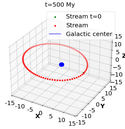
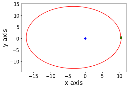
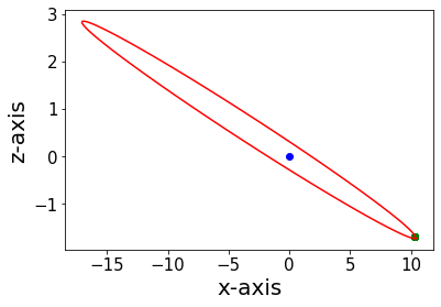
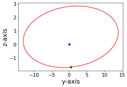
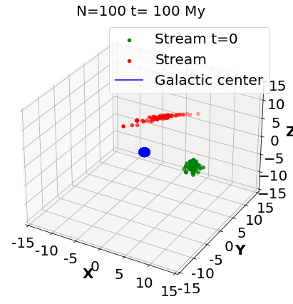
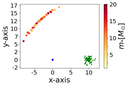
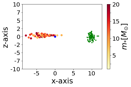
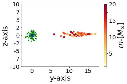
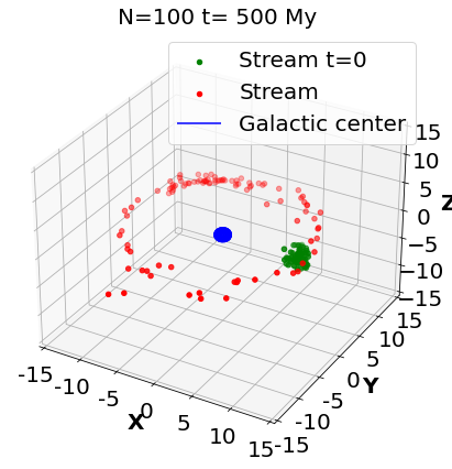
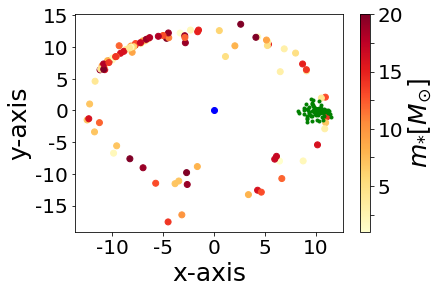
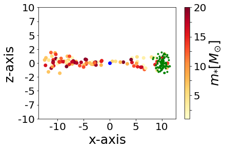
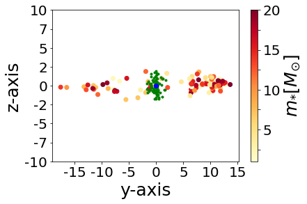
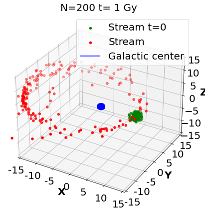
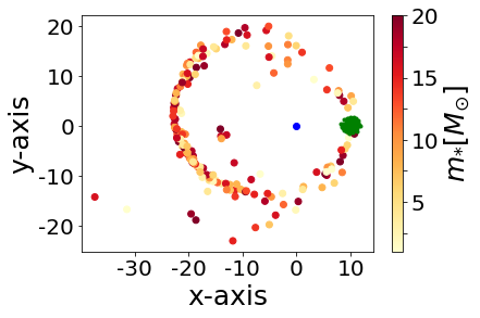
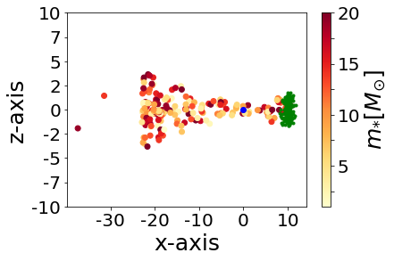
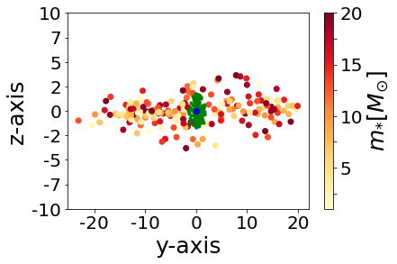
Figure 1: Top row: movement of a single star around a spherical gravitational source akin to the Milky Way. Next three rows: generation of a tidal stream around the same source, measured at times $t=80$ $My$, $t=100$ $My$ and $t=1$ $Gy$. The initial cluster has a radius of 1 kpc and is at a distance of 10 kpc from the galactic origin of coordinates. Member stars have slightly different velocities $v_{*}=220{\rm kpc}\pm\Delta v$ due to the additional random $\Delta v$.

The discussion just presented in subsection 2.2 refers to the torsion of one test body moving in a central field. So if the body lost dust grains forming a kind of contrail, its shape through space would be a planar curve. But stellar streams are not quite of this nature, rather the result of the tidal stretching of a globular cluster or dwarf galaxy Noreña et al. (2019). Since each star or other object in the cluster starts off at a different height $z$ respect to the galactic plane, its orbit around the center of force lies on a slightly different plane, the effect being that the cluster, additionally to stretching, contorts, with the upper particles passing under the center of mass and becoming the lower ones with each half orbit.

We here show that this effect is negligible and the torsion of a stream around a central potential can safely be neglected, as the center of mass of the stream follows one of the trajectories of subsection 2.2, with $\tau=0$. Rather than entangling the discussion in detailed theory, a couple of simple simulations will serve to illustrate the point.

We simulate a globular cluster of $N$ (typically up to a few hundred) pointlike stars with a certain mass $m_{*}$ and common initial velocity ${\bf v}_{*}\sim 220$kpc, randomly distributed at $t=0$ over a sphere of radius $R_{0}$ (of order one or few kpc, typically; in the following simulation, 2 kpc) at a distance $|r|$ from the galactic center (of order 10 kpc in the following example). An additional random velocity kick $\Delta v_{0}=Gm_{\rm cluster}/2r_{0}$ in a random direction is given.

We then let it evolve under the gravitational force of the central source with mass $M\in(10^{9},10^{11})$, standing for a galactic bulb or a spherical DM halo, and we allow for a correction due to the inner binding forces of the cluster. This is small because the random masses are taken in the interval $m_{*}\in(0,20)M_{\odot}$ and thus their mutual interactions are orders of magnitude smaller than those with the galactic center. The constant $GM$ of the central source can conveniently be eliminated in terms of the typical velocity of circular orbits around the galactic center, from orbital equilibrium $v_{\rm rot}^{2}/r=GM/r^{2}$. For the Milky Way this is typically 220 km/s.

The positions of the stellar objects are updated in Cartesian coordinates. The position is updated using Euler’s Method with time step $\Delta t=t_{f}/N_{t}$, with the velocity updated via a once-improved Euler step,

$$x_{j+1}^{i} = x^{i}_{j}+\Delta tv^{i}_{j}\thinspace\thinspace\thinspace\thinspace\text{for i=1,2,3}$$ (9)

$$v^{i}_{j+1} = v^{i}_{j}+\frac{1}{2}\Delta tf^{i}({\bf x}_{j}+\frac{1}{2}h{\bf v}_{j})\thinspace\thinspace\thinspace\thinspace\text{for i=1,2,3}$$ (10)

where $f^{i}$ is the function yielding each component’s acceleration.

The acceleration is calculated at each step from standard formulae

$$a_{i=1,2,3}= - GM\frac{x^{i}}{(x^{2}+y^{2}+z^{2})^{3/2}}$$ (11)

$$- \sum^{N-1}_{j=1}G\frac{m_{j}x^{i}}{((x-x_{j})^{2}+(y-y_{j})^{2}+(z-z_{j})^{2})^{3/2}}\ .$$

The first line of this expression is the acceleration caused by the central spherical source, and the second is the force that attempts to bind the stellar-stream stars together (and that is too weak to avoid the tidal stretching).

We show the simulation in Fig. 1. The concentrated green points mark the initial cluster at $t=0$ in all panels (three dimensional views as well as Cartesian projections as marked in the axes). The evolved cluster at later times, the cloud of red dots, is seen to stretch under tidal tensions. In the panels of the two right columns we see that, due to the initial random velocity in the $z$ direction, the cloud expands and compresses along the vertical $OZ$ axes. But the left colum shows that the stream remains near the (slightly tilted) plane that contains the initial velocity, without developing out-of-plane motion, and therefore no measurable torsion.

3 Orbits around elongated potentials and $\tau\neq 0$

3.1 Movement around a Newtonian cylindrical source

We now move on to quickly show how torsion is expected to look for an orbit around a perfectly cylindrical source of gravity, in a discussion paralleling that of subsection 2.2. We naturally employ cylindrical coordinates $(\rho,\varphi,z)$, so that

$${\bf r} = \rho\hat{\boldsymbol{\rho}}+z\hat{\bf z}$$ (12)

$${\bf r}^{\prime} = \rho^{\prime}\hat{\boldsymbol{\rho}}+\rho\varphi^{\prime}\hat{\boldsymbol{\varphi}}+z^{\prime}\hat{\bf z}$$ (13)

$${\bf r}^{\prime\prime} = (\rho^{\prime\prime}-\rho\varphi^{{}^{\prime}2})\hat{\boldsymbol{\rho}}+(2\rho^{\prime}\varphi^{\prime}+\rho\varphi^{\prime\prime})\hat{\boldsymbol{\varphi}}+z^{\prime\prime}\hat{\bf z}$$ (14)

where in the acceleration we recognize, from left to right, the radial, centrifugal, Coriolis, azimuthal and vertical accelerations, respectively. The force law is the same as that for a line of charge in electromagnetism, except of course with the constant replaced, so that in terms of the linear mass density $\lambda$,

$${\bf r}^{\prime\prime}=\frac{\bf F}{m}=\frac{-2G\lambda}{\rho}\hat{\boldsymbol{\rho}}+0\cdot\hat{\boldsymbol{\varphi}}+0\cdot\hat{\bf z}\ .$$ (15)

Comparing with the general form in Eq. (14) we recover $z^{\prime\prime}=0\implies z^{\prime}={\rm constant}$ (reflecting translational invariance along the $OZ$ axis) and $\rho^{2}\varphi^{\prime}={\rm constant}$ so that the third component $l_{z}/m$ of angular momentum per unit mass is conserved just as in the central force problem. However, now the direction of ${\bf l}$ is not conserved, so that the binormal vector changes and one expects a torsion. To obtain it, start from Eq. (15) and take a further derivative to obtain

$${\bf r}^{\prime\prime\prime}=\frac{-2G\lambda}{\rho}\left(-\frac{\rho^{\prime}}{\rho}\hat{\boldsymbol{\rho}}+\varphi^{\prime}\hat{\boldsymbol{\varphi}}\right)$$ (16)

(valid for the Newtonian force with cylindrical symmetry only). Calculating the cross-product of Eq. (13) and Eq. (15), while using the righthandedness of the trihedron $(\hat{\boldsymbol{\rho}},\hat{\boldsymbol{\varphi}},\hat{\bf z})$ to evaluate each basis vector product, yields

$${\bf r}^{\prime}\times{\bf r}^{\prime\prime}=(-2G\lambda)\left[-\varphi^{\prime}\hat{\bf z}+\frac{z^{\prime}}{\rho}\hat{\boldsymbol{\varphi}}\right]\ .$$ (17)

Next we take the scalar product with ${\bf r}^{\prime\prime\prime}$ and evaluate Eq. (5) to obtain the torsion, yielding

$$\tau=\frac{z^{\prime}\varphi^{\prime}}{(\rho\varphi^{\prime})^{2}+z^{{}^{\prime}2}}=\frac{1}{\rho}\frac{v_{z}v_{\varphi}}{v_{\varphi}^{2}+v_{z}^{2}}$$ (18)

that we have cast in an easier to remember form in the second expression. Clearly, for there to be a torsion we need both azimuthal and vertical velocities (so stellar streams in the galactic plane are not sensitive, as expected). Additionally, because $|v_{z}v_{\varphi}|\leq v_{z}^{2}+v_{\varphi}^{2}$, torsion belongs to the interval $\tau\in[-\rho^{-1},\rho^{-1}]$, so its maximum magnitude is controlled by the distance from the stellar stream segment to the galactic axis.

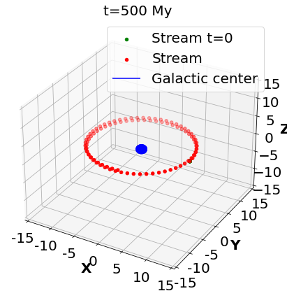
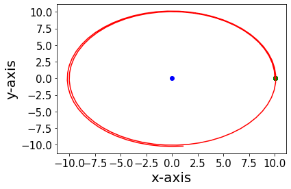
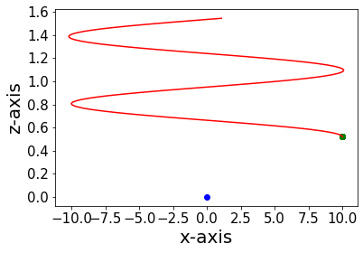
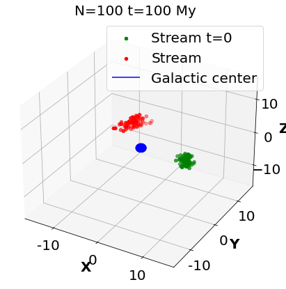
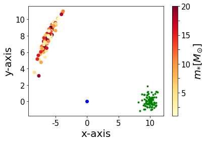
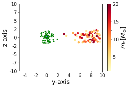
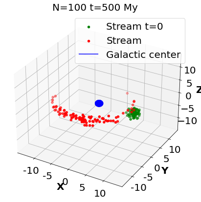
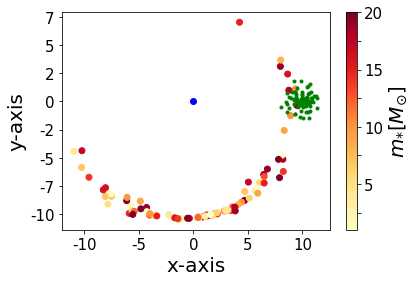
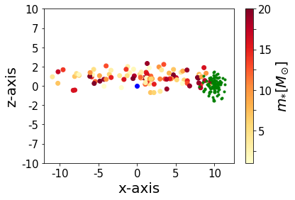
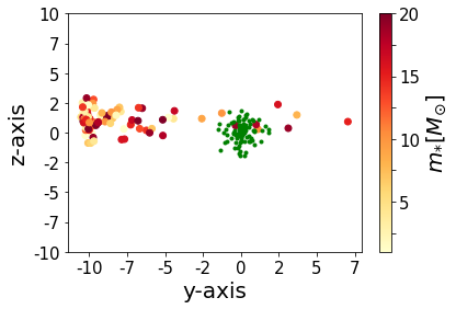
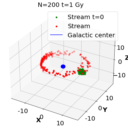
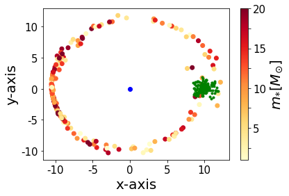
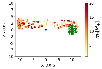
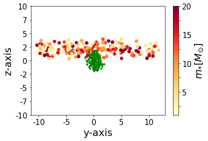
Figure 2: As in Fig. 1 but with a cylindrical gravitational source. The top row tracks the motion of a particle around the cylindrical source, following a spiral trajectory with an initial $v_{z}=$ 2 km/s. From top to bottom, rows 2 to 4 correspond to a cluster of stars with similar initial velocity seen at times $t=80$ $My$, $t=100$ $My$ and $t=1$ $Gy$.

3.2 Simulation of an N-point stellar stream around a cylindrical source

Next we proceed to repeat the exercise of subsection 2.3 with the same starting data, but replacing the central spherical Newtonian source by a cylindrical source. The force in Eq. (11) needs to be replaced, so that

$$a_{i=1,2}= - 2G\lambda\frac{x^{i}}{x^{2}+y^{2}}$$

$$- \sum^{N-1}_{j=1}G\frac{m_{j}x^{i}}{((x-x_{j})^{2}+(y-y_{j})^{2}+(z-z_{j})^{2})^{3/2}}$$

$$a_{i=3}= - \sum^{N-1}_{j=1}G\frac{m_{j}x^{i}}{((x-x_{j})^{2}+(y-y_{j})^{2}+(z-z_{j})^{2})^{3/2}}.$$ (20)

Its first term is the acceleration caused by the cylindrical gravitational source (that along the $OZ$ axis being zero by translational symmetry). Its linear mass-density $\lambda=M/L$ is obtained from the typical rotation curve around a galaxy $v_{rot}=\sqrt{2G\lambda}$ Llanes-Estrada (2021). The second term of Eq. 3.2 is, again, the correction due to the tiny binding of the stellar streams stars among themselves, together with Eq. (20). An example can be seen in Fig 2, where all trajectories seem to overall fall in a plane.

The result of the analogous simulation is represented in Fig. 2. If the starting velocity profile was perfectly set in the $XY$ plane perpendicular to the cylinder, the torsion would still be zero as per Eq. (18). We give it a slight tilt and then the orbit starts behaving as a helix (which can be appreciated in the bottom row, where the originally compact cluster of stars has, after 1 Gyr, become a tidal stream that does not close on itself but ascends in a spiral, showing a small torsion). We detail in Fig 3 how the effect becomes more noticeable upon rigging the initial star cluster with a larger speed along the OZ axis.

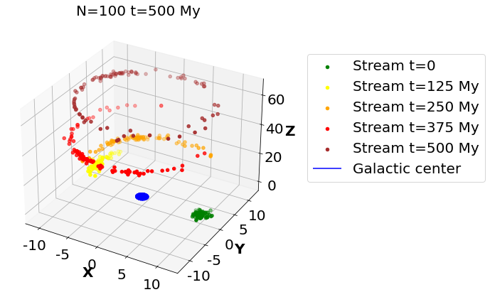
Figure 3: We show the spread of a 100-body stellar cluster with initial vertical speed $v_{z}=50$km/s after $t=$ 0, 125, 250, 375 and 500 My. The resulting stream at different times clearly shows an upward advancing helix moving around the z-axis.

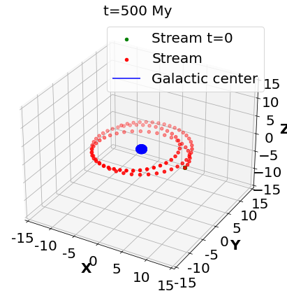
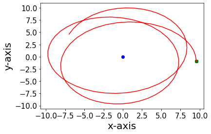
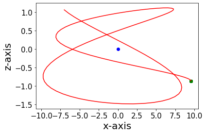
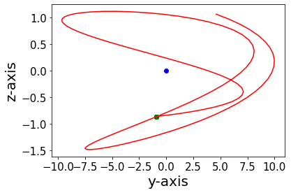
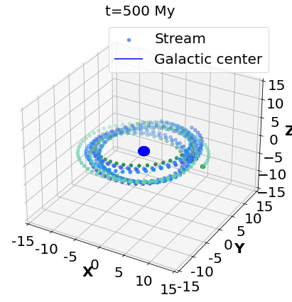
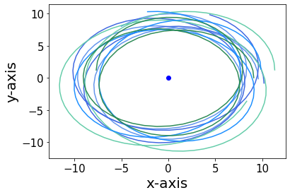
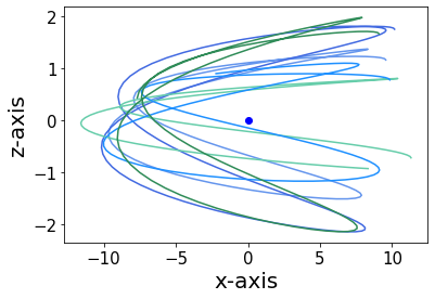
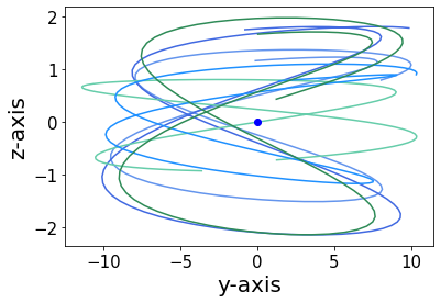
Figure 4: In the first row we represent the trajectory of a pointlike mass with initial velocity $v_{z}=$5 km/s around a source combining both a sphere and a cylinder. The second row extends this to simultaneously show the motion of five stars.

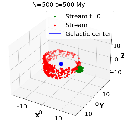
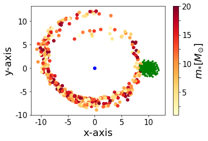
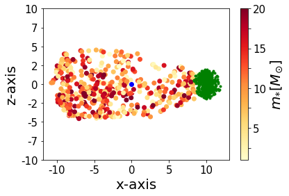
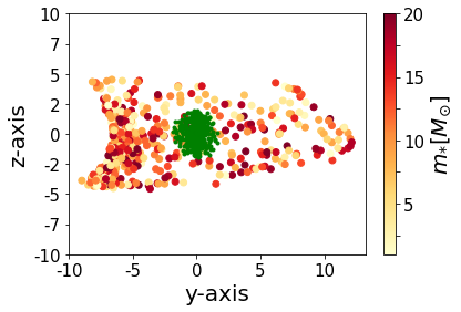
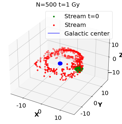
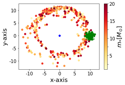
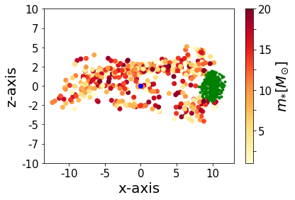
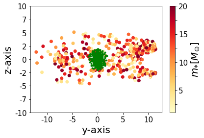
Figure 5: Formation of a stellar stream from initial cluster orbiting a combined spherical+cylindrical source as in Fig. 4 for two times $t=500$ My and $t=1$ Gy.

3.3 Sphere and cylinder with additional $v_{z,0}$

To close this section, we will combine together both types of sources, a sphere (akin to a visible-matter galactic bulb) and a cylinder (mimicking an elongated DM halo). For the sphere we take the typical mass of a galaxy $M_{s}\in(10^{9},10^{12})M_{\odot}$ Busha et al. (2011), Binney & Tremaine (1987) and for the cylinder we use the expression for the linear mass density that we obtain from the asymptotic velocity at large $r$ in the rotation curve $v_{rot}$ of the Milky Way, as exposed in the previous section 3.

The updated expression for the acceleration of the stars in the stream is obtained by combining Eqs. (11) and (3.2), that is,

$$z^{\prime\prime} = -\frac{v_{0}^{2}}{|{\bf r}|^{3}}z$$ (21)

$${\bf r}_{\perp}^{\prime\prime} = -\frac{|{\bf v}|^{2}}{|{\bf r}_{\perp}|^{2}}{\bf r}_{\perp}-\frac{v_{0}^{2}}{|{\bf r}|^{3}}{\bf r}_{\perp}$$ (22)

where $v$ is taken from the galactic rotation velocity when it has flatted out at large $r$, and $v_{0}$ estimated from the visible mass.

We have added a small but appreciable contribution to the initial velocity in the $z$ direction, $v_{*}$ = $(220+\Delta v,\Delta v,5+\Delta v)$ km/s to induce sufficient vertical, out of plane motion that will generate torsion as per Eq. (18).

In Fig. 4 we clearly observe traits of the motion around cylinder+sphere sources as described in Llanes-Estrada (2021). Along the symmetry $OZ$ axis, a star will describe harmonic oscillations between the two hemispheres due to the Newtonian pull of the spherical part of the distribution acting towards the center (unless it is provided with escape velocity, in which case it will approach an asymptotic trajectory, a helix around the $OZ$ axis). The orbit on the $XY$ plane is not closed due to the additional $1/r$ force. The net effect in three dimensions can be seen as a precession of the orbital plane around the $OZ$ axis, with the trajectory creating complicated helicoidal patterns.

The simulation in Fig. 5 reflects this and clearly shows the appearance of nonvanishing torsion in the stellar streams (see particularly the three-dimensional rendering in the left bottom plot).

3.4 Torsion in a galaxy with a spherical halo and a galactic plane

We wish to have a reference for a minimum torsion that we would consider “normal” in order of magnitude, so that if extensive studies of stellar streams show that their torsion exceeds that level, one could reject the hypothesis of a spherical halo.

For this purpose we propose here a toy model in which the halo is taken spherical, but we add a disk component. This adds a vertical (not radial) velocity outside of the galactic plane that points towards it.

The simplest (and coarsest) such model takes the galactic disk as being uniform and infinite. This is a reasonable approximation only for streams that do not elevate too much along the $OZ$ axis; otherwise it provides an upper bound to a more realistic torsion (since such additional vertical force will always be larger than that of a finite disk, whose effect will fall off with $z$). In that case, observed torsions above this bound would still entail an incompatibility with a spherical halo to be studied further.

Therefore, in this minimum-torsion model we take the acceleration as

$$a_{i=1,2}= - GM\frac{x^{i}}{(x^{2}+y^{2}+z^{2})^{3/2}}$$

$$a_{3}= - GM\frac{z}{(x^{2}+y^{2}+z^{2})^{3/2}}-2\pi G\sigma{\rm sign}(z)\ .$$ (23)

In this equation, $\sigma$ is a surface mass density for the disk, in the range $50-100M_{\odot}/$parsec² which is a usual estimate Kuijken & Gilmore (1989), Kuijken & Gilmore (1991) at 8 kpc from the galactic center.

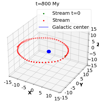
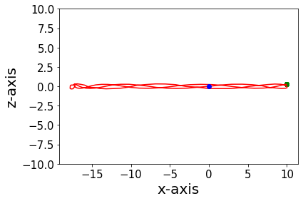
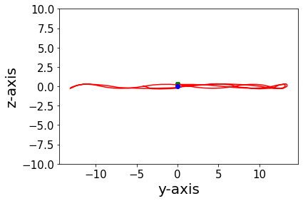
Figure 6: Simulation of a small tidal stream in the presence of a typical non-spherical galactic source, here the galactic plane model of Eq. (23). From top to bottom: three-dimensional view, $XZ$ and $YZ$ sections.

Fig. 6 shows the characteristic wobbling of movement near the galactic plane caused by the planar disk, which is qualitatively consistent with Cordoni et al. (2021).

We can provide an analytical estimate of the torsion following the now familiar reasoning. Since an instantaneous velocity that is parallel to any of the three coordinate vectors of the cylindrical base $\{\hat{\boldsymbol{\rho}},\hat{\boldsymbol{\varphi}},\hat{\mathbf{z}}\}$ will display zero torsion, we take a trajectory combining two of them,

$${\bf r}^{\prime}=v_{\varphi}\hat{\boldsymbol{\varphi}}+v_{z}\hat{\mathbf{z}}\ .$$ (24)

Multiplying by the acceleration in Eq. (3.4) we obtain

$${\bf r}^{\prime}\times{\bf r}^{\prime\prime}=\frac{GM\rho}{r^{3}}(v_{\varphi}\hat{\mathbf{z}}-v_{z}\hat{\boldsymbol{\varphi}})-Gv_{\varphi}\left(\frac{M}{r^{3}}z+(2\pi)\sigma{\rm sign}(z)\right)\hat{\mathbf{\rho}}\ .$$ (25)

To construct the determinant $(({\bf r}^{\prime}\times{\bf r}^{\prime\prime})\cdot{\bf r}^{\prime\prime\prime})$ necessary for the torsion, we evaluate the third derivative outside the galactic plane (where it is undefined),

$${\bf r}^{\prime\prime\prime}=-\frac{GM}{r^{2}}\left(\hat{\bf r}^{\prime}-\frac{2}{r}(\hat{\bf r}\cdot\mathbf{r}^{\prime})\hat{\mathbf{r}}\right)$$ (26)

that is in the plane given by position and velocity, employing

$$\hat{\bf r}^{\prime} = \frac{1}{r}\left({\bf v}-(\hat{\bf r}\cdot{\bf v})\hat{\mathbf{r}}\right)$$ (27)

$$= \frac{1}{r}\left(v_{\varphi}\hat{\boldsymbol{\varphi}}+v_{z}\hat{\mathbf{z}}-\frac{zv_{z}}{r^{2}}(\rho\hat{\boldsymbol{\rho}}+z\hat{\mathbf{z}})\right)\ .$$

A slightly tedious but straightforward calculation then yields

$$\tau=\frac{-6\pi\,(M\sigma)\,(|z|\rho)\,(v_{z}v_{\varphi})}{v_{\varphi}^{2}(M^{2}r+4\pi\sigma M|z|r^{2}+4\pi^{2}\sigma^{2}r^{5})+v_{z}^{2}M^{2}\rho^{2}/r}\ .$$ (28)

The numerator has mechanical dimensions of a squared momentum, and the denominator of squared momentum times length, yielding the correct $1/L$ dimensionality of the torsion. Moreover, the structure of the denominator shows that in the presence of a spherical source ($M$) alone, or a plane ($\sigma$) alone, the torsion vanishes as it should. Likewise, both components of the velocity have to be nonvanishing as in Eq. (18) for the cylindrical source; and the torsion is null both on the galactic plane ($z=0$) and on its perpendicular axis through the center of the sphere ($\rho=0$). We can then numerically evaluate Eq. (28) to obtain the floor value of the torsion that we should expect to be able to use in the galaxy. Taking into account that the galactic plane is not infinite so that the elevation $z$ will yield a diminishing multipolar field, it may be that galactic torsions from a spherical halo plus disk are even smaller; what we mean by this estimate is that those streams that may be found with larger values need to be further investigated as they may be teaching us something about the dark matter halo or about dark matter inhomogeneities.

Employing z$\sim 1$kpc, $\rho\sim r\sim 10$ kpc, $v_{z}\sim v_{\varphi}\sim 220$ km/s (to take the most conservative floor to the torsion), $M\sim 10^{12}\ M_{\odot}$, and $\sigma\sim 10^{8}\ M_{\odot}/$kpc² as already discussed, the denominator of Eq. (28) is dominated by the $M^{2}$ terms, with the $\sigma r^{2}$ correcting $M$ only at the percent level. With these numbers we then find $\tau\sim-9\cdot 10^{-4}$kpc^-1.

We then conclude that torsions of stellar streams below $10^{-3}$ in our galaxy can be explained without resort to deformed dark matter haloes or exotic phenomena. Of the few streams presently known, most present torsions at this level or below and are thus of no further interest for this application of the shape of the haloes. It is those that reach $\tau$ at the percent level that deserve further scrutiny to bear on the halo shape, among the ones known and in future searches for streams.

4 Stellar streams in the Milky Way and their torsion

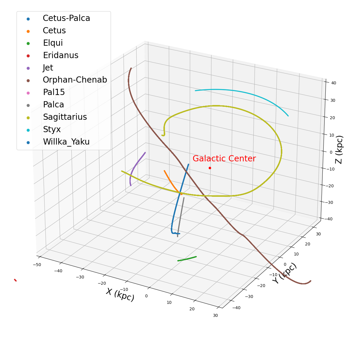
Figure 7: Trajectories in galactocentric coordinates for some of the MW outer streams, extracted from Mateu (2023).

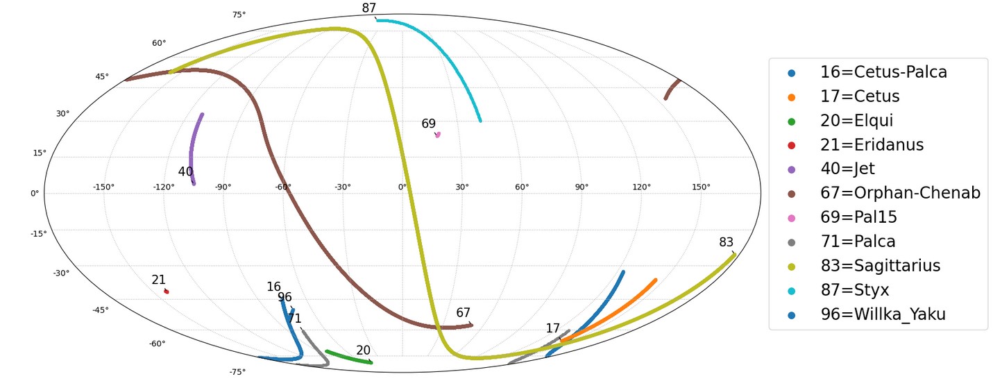
Figure 8: Trajectories for some of the MW outer streams in Mollweide projection, extracted from Mateu (2023).

In this section we finally turn to some of the known stellar streams in the Milky Way. We select as relevant those found at distances $d>30$ $kPc$ from the galactic center, so that the internal structure of the galaxy, such as the disk and spiral arms, produces the minimum possible alteration in the stream. These streams, see Figs. 7 and 8, have been extracted from Mateu (2023). The intention in this section is to extract the value of the torsion of the parametrized stream curves with Eq. (5) and check for their vanishing (or not).

We have taken two of the streams out of further consideration, namely those at Orphan-Chenab and Styx. The reason is that they may be influenced by gravity sources outside the MW. Due to the proximity of the Large Magellanic Cloud (LMC) to our galaxy, the streams in its periphery in the angular direction of that cloud could suffer alterations due to this additional source of gravity Conroy et al. (2021), Lilleengen et al. (2022).

To obtain the torsion of the curves following the stream we have opted for employing a smooth (polynomial) parametrization. Therefore, we first fit each of the galactocentric Cartesian coordinates tracking the individual streams in the data compilation of Mateu (2023) to order-four polynomial parametric curves. The parameter that describes each curve takes values in the interval $k\in[0,5]$. The generic parametrization and a plot of each of them for the various streams, projected over the Cartesian axes, are relegated to the appendix, see Eq. (30) and Fig. 10. This parameter $k$ is an arbitrary coordinate that can be converted to arc length, that has clearer geometric significance, by means of

$$s=\int\sqrt{\sum^{3}_{i=1}\left(\frac{dx^{i}}{dk}\right)^{2}}dk\ ;$$ (29)

the derivatives in Eq. (5) are to be taken respect to the parameter $k$, in general, or $s$, if a change is variables is effected (the outcome is the same, of course) to obtain the torsion.

To work with the streams in the database we use the galstream library and to perform the fits we use the polyfit command in the numpy module within a standard Python installation.

A word about the uncertainty in this extraction is warranted. The data points for the extracted stream trajectories are quoted without errors in the original reference of Mateu (2023), perhaps because they are rather small; thus, the uncertainty of our parametric reconstruction stems in its entirety from the interpolation of Eq. (30) until uncertainties in the data are compiled.

After the reconstruction of the parametric curves in Fig. 10, we can obtain the expression for the torsion of each curve $r=(x,y,z)$ using once more Eq. (5) $\tau=\frac{Det(r^{\prime},r^{\prime\prime},r^{\prime\prime})}{||r^{\prime}\times r^{\prime\prime}||^{2}}$, where the derivative is taken respect to the $k$ parameter, ${}^{\prime}=d/dk$. We analytically express the derivatives in terms of the polynomial parametrization and then evaluate them as function of the $k$ parameter that we used for the fit, taking values from 0 to 5. Because the torsion is parametrization independent, the torsion can also be given as function of the arclength $\tau(s)$ calculating the derivatives respect to either of $k$ or $s$.

The torsion along the curve shows significant variations in some of the streams in Fig. 9, such as Cetus-Palca, Cetus, Elqui, Jet and Pal15. In Table (1) we quantify this variation between minimum and maximum values in the relevant streams that we look at. Reasons for this variation might be a non-spherical gravitational source and also the interaction with other gravitational sources different from the overall galactic field.

Stream	$CV=\frac{\tau_{max}-\tau_{min}}{\tau_{min}}$
Cetus-Palca	0.94
Cetus	1904.7
Elqui	2.67
Eridanus	2.04
Jet	1.00
Pal15	2.04
Palca	1.63
Sagittarius	1.00
Willka-Yaku	2.17

Table 1: Coefficient of variation (CV) with respect to background for the torsion along each stream.

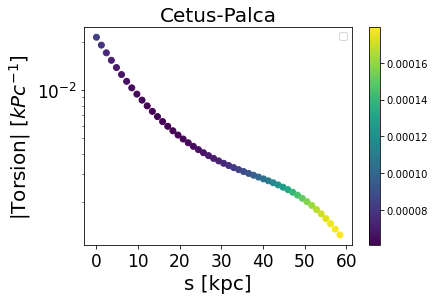
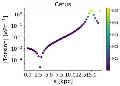
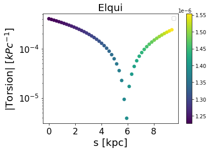
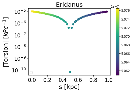
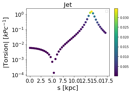
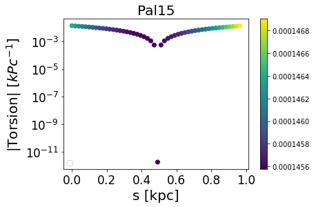
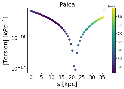
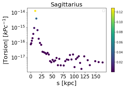
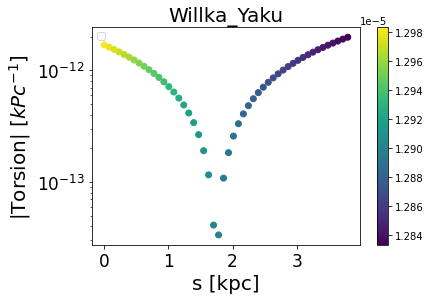
Figure 9: Torsion (in units of kPc^-1) of the streams considered in this work with uncertainties from the error propagation of the calculated torsion in Eq. (5) given with the color code (the lighter shades stand for the largest uncertainties). The errors of the bottom–row streams (Palca, Sagitarius and Willka Yaku) are very large in comparison to any torsion, so their $\tau$ is to be taken compatible with zero within those errors.

Because torsion (as curvature) has dimensions of inverse length, we would expect stellar streams to perhaps show an inverse relation with respect to their distance from the galactic center, as defined in Eq. (5). Irrespectively, in a galaxy such as the Milky Way the torsion of galactic streams should have a characteristic scale of $(10$ kPc$)^{-1}$. As per the discussion around Eq. (18), where we established $\tau\in\left[-\frac{1}{\rho},\frac{1}{\rho}\right]$, our selection of streams at 30 kpc or more means that we would consider values of the torsion of order 0.03 in units of inverse kiloparsec to be sizeable and very different from zero. Also, as per the discussion below Eq. (28), those above 0.001 could perhaps carry interesting information about the DM distribution.

Turning to the data, the torsions that we seem to observe in the MW streams show orders of magnitude variation, with some factors of 20 or more larger than the expected scale and others totally negligible, perhaps due to their being close to lying on the galactic plane or moving in an $OZ-r$ vertical plane, so that $v_{z}$ or $v_{\varphi}$, respectively, are small.

The Jet and Cetus streams have sizeable $OZ$-axis displacements and consistently with Eq. (18) they present sizeable torsion.

5 Conclusions and outlook

The problem of galactic rotation curves suggests that galaxies are surrounded by significant amounts of dark matter, and the overall shape of these sources is yet to be ascertained. Whereas spherical DM distributions around galaxies have to be fine-tuned to explain the flatness of rotation curves, a cylindrical (or, generally, prolate) DM source can naturally explain the flattening of rotation curves. This avoids the fine-tuning of spherical DM haloes to precisely follow the $1/r^{2}$ fall-off for a large swath of $r$ values. Observables inside the galactic plane cannot however distinguish between spherical (though fine tuned) and cylindrical/elongated gravitational sources, but out-of-galactic-plane information could provide new strong discriminants.

The stellar streams around the Milky Way have been extensively investigated for a while now, and are still nowadays a relevant subject of research. The trajectory followed by streams can be used as a tool to infer the geometry of these gravitational sources. Orbits can be characterized by their torsion according to Eq.  (5); around a central potential orbits move in a plane and are expected to be torsionless (see Fig. 1). In addition, test masses around cylindric sources are expected to follow helical orbits in which the torsion is non-zero (see Fig. 2). Another approach is to consider an ellipsoid-shaped halo, which is not perfectly cylindrical but rather elongated. The expected orbit of the streams would arise from the combination of the orbits around central potentials and the helical orbits around cylinders, as is seen in Fig. 4.

The streams of the Milky Way have been a subject of research for a considerable time span, and many of the objects that constitute these streams have been catalogued. From a reconstruction of the orbits followed by these streams we infer the torsion caused by the gravitational source in Fig. 9. In this work we only consider those streams that seem to be far enough away from the galactic center to (1) avoid large effects from the baryonic component of the galaxy and (2) have a bird’s eye view of the DM halo from outside a large fraction thereof. From the extraction of the torsion we see that it is non-negligible in some of the streams considered.

From our evaluation of the torsion we do not dare favor one or another interpretation of the DM halo shape in view of current data; this article should be seen as a proposal for a new observable, $\tau$, and a first exploratory study. We do find streams with significant torsion, but that have also with significant variability, which begs for further understanding.

In future observational work it might be interesting to actively seek streams that show both vertical motion (along the axis perpendicular to the MW plane) and also azimuthal motion around that axis, as those with large $v_{z}$ and $v_{\varphi}$ will be most sensitive to the torsion. Should those streams show trajectories that are compatible with lying on a plane (zero torsion), a spherical halo will be prefered. Should they however appear helicoidal, with nonnegligible torsion, they would be pointing to an elongated DM halo.

Streams that may be detected in nearby galaxies carry the same information about their respective haloes.

Finally, other observables can bear on the overall shape of the halo, and we are considering investigating the shape-sensitivity of the gravitational lensing of both electromagnetic and gravitational radiation.

6 Appendix

The parametrization $(x(k),y(k),z(k))$ that we employ reads

$$x^{i}(k)=a_{i}k^{4}+b_{i}k^{3}+c_{i}k^{2}+d_{i}k+e_{i}\thinspace\thinspace\thinspace\text{for i=1,2,3}.$$ (30)

It is idle to try to relate $k$ to a Newtonian time $t$ since, not knowing a priori the dynamics of the system, it is unknown at which time a star was at what position along its trajectory. Only the instantaneous (present) geometry of the stream is known with certainty, and therefore an arbitrary parameter $k$ (or the arc length after computing it) should suffice.

In Figs. 10 and 11 we then display the polynomial fit to each one of the streams considered in this work using Eq. (30) by plotting the parametrization $(x(k),y(k),z(k))$.

In particular, note that the Jet and Cetus streams, that show the largest torsions in Fig. 8 are well described by the simple $4^{\rm th}$ order polynomial fit and have no structure worth mentioning.

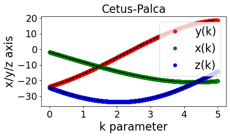
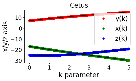
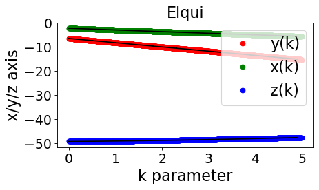
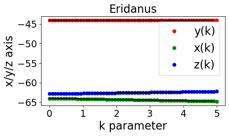
Figure 10: Reconstruction of the parametric curves using Eq. (30).

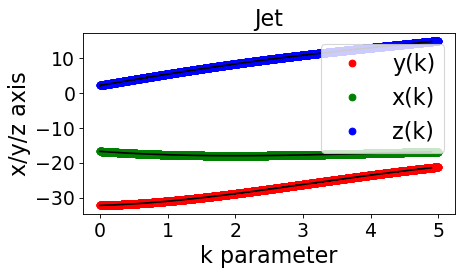
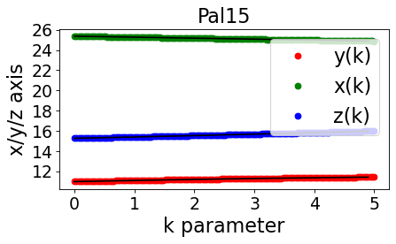
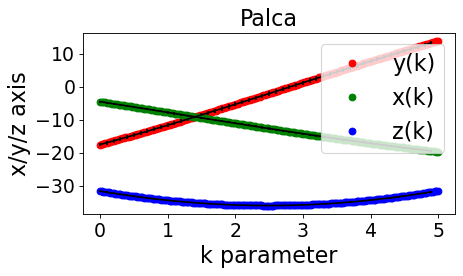
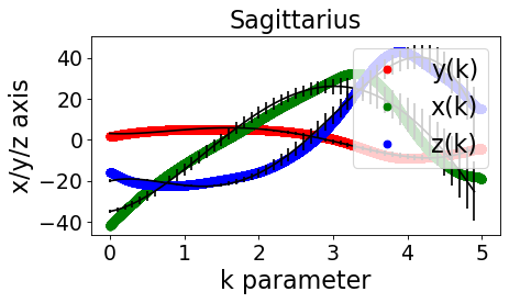
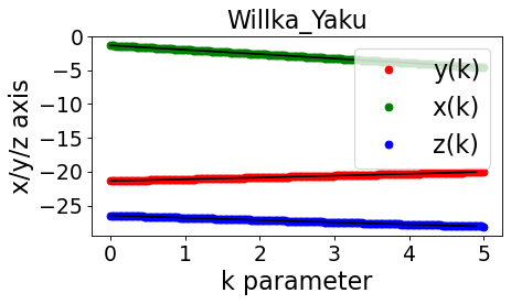
Figure 11: Reconstruction of the parametric curves using Eq. (30).