HEAL-SWIN: A Vision Transformer On The Sphere

Abstract

High-resolution wide-angle fisheye images are becoming more and more important for robotics applications such as autonomous driving. However, using ordinary convolutional neural networks or vision transformers on this data is problematic due to projection and distortion losses introduced when projecting to a rectangular grid on the plane. We introduce the HEAL-SWIN transformer, which combines the highly uniform Hierarchical Equal Area iso-Latitude Pixelation (HEALPix) grid used in astrophysics and cosmology with the Hierarchical Shifted-Window (SWIN) transformer to yield an efficient and flexible model capable of training on high-resolution, distortion-free spherical data. In HEAL-SWIN, the nested structure of the HEALPix grid is used to perform the patching and windowing operations of the SWIN transformer, resulting in a one-dimensional representation of the spherical data with minimal computational overhead. We demonstrate the superior performance of our model for semantic segmentation and depth regression tasks on both synthetic and real automotive datasets. Our code is available at https://github.com/JanEGerken/HEAL-SWIN.

1 Introduction

Figure 1: Our HEAL-SWIN model uses the nested structure of the HEALPix grid to lift the windowed self-attention of the SWIN model onto the sphere.

High-resolution fisheye cameras are among the most common and important sensors in modern intelligent vehicles [1]. Due to their non-rectilinear mapping functions and large field of view, fisheye images are highly distorted. The traditional approach for dealing with this kind of data is nevertheless to use standard (flat) convolutional neural networks which are adjusted to the distortions introduced by the mapping function and either preprocess the data [2, 3, 4, 5, 6, 7] or deform the convolution kernels [8]. However, these approaches struggle to capture the inherent spherical geometry of the images since they operate on a flat approximation of the sphere. Errors and artifacts arising from handling the strong and spatially inhomogeneous distortions are particularly problematic in safety-critical applications such as autonomous driving. Furthermore, certain downstream tasks like 3D scene understanding inherently require spherical information, such as the angle under which an object is detected, which needs to be extracted from the predictions of the model.

In this paper we show that projecting spherical data to the plane and learning on distorted data, only to project the resulting predictions back onto the sphere, introduces considerable performance losses. We demonstrate this for standard computer vision tasks from the autonomous driving domain. We therefore argue that, for applications that require a very precise 3D scene understanding, computer vision models that operate on fisheye images should be trained directly on the sphere in order to avoid the significant losses associated with flat plane projections.

Optimizing on the sphere is an approach taken by some models [9, 10, 11], which lift convolutions to the sphere. These models rely on a rectangular grid in spherical coordinates, namely the Driscoll–Healy grid [12], to perform efficient Fourier transforms. However, this approach has several disadvantages for high-resolution data: First, the sampling in this grid is not uniform but much denser at the poles, necessitating very high bandwidths to resolve fine details around the equator. Second, the Fourier transforms in the aforementioned models require tensors in the Fourier domain of the rotation group $\mathrm{SO}(3)$ which scale with the third power of the bandwidth, limiting the resolution. Third, the Fourier transform is very tightly coupled to the input domain: If the input data lies only on a half-sphere as in the case of fisheye images, the definition of the convolutional layers would need to be changed to use this data efficiently.

As a novel way of addressing all of these problems at the same time, we propose to combine an adapted vision transformer with the Hierarchical Equal Area iso-Latitude Pixelisation (HEALPix) grid [13]. The HEALPix grid was developed for capturing the high-resolution measurements of the cosmic microwave background performed by the MAP and PLANCK satellites and features a uniform distribution of grid points on the sphere which assosciates the same area to each pixel. This is in contrast to most other grids used in the literature like the Driscoll–Healy grid or the icosahedral grid. Furthermore, due to its widespread use in the astrophysics- and cosmology communities, efficient implementations in C++ of the relevant computations are readily available as a Python package [14].

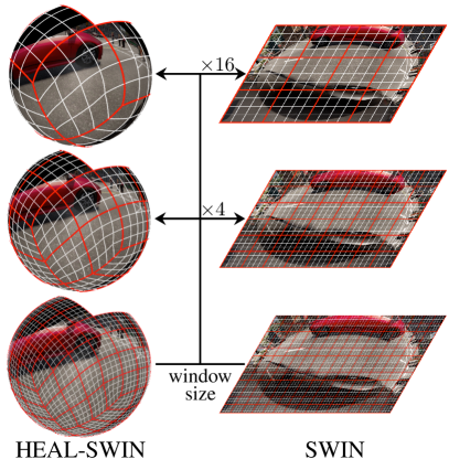
In our model, which we call HEAL-SWIN, we use a modified version of the Hierarchical Shifted-Window (SWIN) transformer [15] to learn directly on the HEALPix grid. The SWIN transformer performs attention over blocks of pixels called windows which aligns well with the nested structure of the HEALPix grid (Figure 1). To distribute information globally, the SWIN transformer shifts the windows in every other layer, creating overlapping regions. We propose two different strategies for shifting windows in the HEALPix grid: Either aligned with the hierarchical structure of the grid or in a spiral from one pole to the other.

Besides their excellent performance, an additional benefit of using a transformer model is that the attention layers do not require a Fourier transform and can therefore easily deal with high-resolution data and with data that covers only part of the sphere, such as images captured by fisheye cameras, resulting in significant efficiency gains. However, our model is not specific to fisheye images but can be trained on any high-resolution spherical data, as provided for instance by satellites mapping the sky or the earth.

Figure 2: Chamfer distance (lower is better) between predicted and ground truth point clouds from depth estimation on SynWoodScape.

Figure 3: Mean intersection over union (higher is better) on the HEALPix grid for semantic segmentation on SynWoodScape.

In order to verify the efficacy of our proposed model, we train HEAL-SWIN on computer vision tasks from the autonomous driving domain, namely depth estimation and semantic segmentation of fisheye camera images. In this domain, high-resolution input images and very precise outputs in terms of 3D information are critical. We show that it is beneficial to optimize on the sphere instead of projecting predictions in the plane onto the sphere to extract the 3D spatial information. To the best of our knowledge, we are the first to treat fisheye images in automotive applications as spherical signals.

We perform fisheye-image-based depth estimation and compare the resulting predicted 3D point clouds to the corresponding ground truth point clouds. In this way, we can assess how well our model captures the 3D information needed for downstream tasks. We show that our model outperforms the corresponding flat model (SWIN transformer) in this setting on the SynWoodScape dataset  [16] of computer-generated fisheye images of street scenes (Figure 3). For the semantic segmentation task, we confirm the superior performance of our model on both the real-world WoodScape dataset [17] and the SynWoodScape dataset when performance is measured on the sphere (Figure 3). Finally, we investigate the performance advantage of our model for different amounts of data by training our segmentation models on subsets of SynWoodScape.

Our main contributions are as follows:

• We argue that in applications involving spherical data, it is essential to take the domain of downstream tasks into account when designing the network architecture. Therefore, we propose to leverage the inherent geometry in the data by training directly on the sphere in cases like depth estimation, where 3D spatial information is required.

• We construct the HEAL-SWIN model for high-resolution spherical data, which combines the spherical HEALPix grid with an adapted SWIN transformer by exploiting their similar hierarchical structures. In particular, we construct windowing and shifting mechanisms for the HEALPix grid which efficiently deal with data that only covers part of the sphere.

• We consider fisheye images in automotive applications for the first time as distortion-free spherical signals. We demonstrate the superiority of this approach for depth estimation and semantic segmentation on both synthetic and real automotive datasets.

2 Related work

The transformer architecture was introduced in [18], extended to the Vision Transformer (ViT) in [19], and further refined in [15] to the Shifted-Window (SWIN) transformer based on attention in local windows combined with window shifting to account for global structure. A first step towards spherical transformer models has been proposed in [20] where various spherical grids are used to extract patches on which the ViT is applied, and in [21] where icosahedral grid sampling is combined with the Adaptive Fourier Neural Operator (AFNO, see [22]) architecture for spatial token mixing to account for the geometry of the sphere. Compared to previous spherical transformer designs, such as [20], our model constitutes a significant improvement by incorporating local attention and window shifting to accommodate high-resolution images in the spherical geometry, without requiring the careful construction of accurate graph representations of the spherical geometry.

The SWIN paradigm has been incorporated into transformers operating on 3D point clouds (e.g. LiDAR depth data) by combining voxel based models (see [23]) with sparse [24] and stratified [25] local attention mechanisms. In [26], spherical geometry is used to account for long range interactions in the point cloud to create a transformer based on local self-attention in radial windows. Closer in spirit to our approach is [27], where the point cloud is projected to the sphere, and partitioned into neighborhoods. Local self-attention and patch merging is then applied to the corresponding subsets of the point cloud, and shifting of subsets is achieved by rotations of the underlying sphere. Our HEAL-SWIN model inherits windowing and shifting from the SWIN architecture, but in contrast to the point cloud based approaches we handle data native to the sphere and use the HEALPix grid to construct a hierarchical sampling scheme which minimizes distortions, allows for the handling of high-resolution data, and, in addition, incorporates new shifting strategies specifically adapted to the HEALPix grid.

Several Convolutional Neural Network (CNN) based models have been proposed to accommodate spherical data. As mentioned above, [9, 10, 11] use an equirectangular grid and implement convolutions in Fourier space, while [28] applies CNNs directly to the HEALPix partitions of the sphere. Other works that consider spherical CNNs combined with the HEALPix grid include [29, 30, 6, 31]. Compared to previous works combining CNNs and the HEALPix grid, the transformer architecture equips our model with the ability to efficiently encode long-range interactions.

3 HEAL-SWIN

We propose to combine the SWIN-transformer [15, 32] with the HEALPix grid [13] resulting in the HEAL-SWIN-transformer which is capable of training on high-resolution images on the sphere. In this section, we describe the structure of the HEAL-SWIN model in detail.

3.1 Background

The SWIN-transformer is a computationally efficient vision transformer which attends to windows that are shifted from layer to layer, enabling a global distribution of information while mitigating the quadratic scaling of attention in the number of pixels.

In the first layer of the SWIN-transformer, squares of pixels are joined into tokens called patches to reduce the initial resolution of the input images. Each following SWIN-layer consists of two transformer blocks which perform attention over squares of patches called windows. The windows are shifted along the patch-grid axes by half a window size, before the attention for the second transformer block is computed. In this way, information is distributed across window boundaries. To down-scale the spatial resolution, two-by-two blocks of patches are periodically merged.

An important detail in this setup is that at the boundary of the image, shifting creates partially-filled windows. Here, the SWIN-transformer fills up the windows with patches from other partially-filled windows and then performs a masked version of self-attention which does not attend to pixel pairs which originated from different regions of the original.

For the depth-estimation and segmentation tasks we consider in this work, we use a UNet-like variant of the SWIN-transformer [33] which extends the encoding layers of the original SWIN-transformer by corresponding decoding layers connected via skip connections. The decoding layers are identical to the encoding layers, only the patch merging layers are replaced by patch expansion layers which expand one patch into a two-by-two block of patches such that the output of the entire model has the same resolution as the input.

In the HEAL-SWIN-transformer, the patches are not associated to an underlying rectangular pixel grid as in the original SWIN-transformer, but to the HEALPix grid on the sphere. The HEALPix grid (Figure 1) is constructed from twelve equal-area quadrilaterals of different shapes which tessellate the sphere and are subdivided along their edges $n_{\mathrm{side}}$ times to yield a high-resolution partition of the sphere into $12\cdot n_{\mathrm{side}}^{2}$ equal-area, iso-latitude quadrilaterals, as illustrated in Figure 1. To allow for a nested (hierarchical) grid structure, $n_{\mathrm{side}}$ needs to be a power of two. The pixels of the grid are then placed at the centers of the quadrilaterals. The resulting positions are sorted in a list either in the nested ordering descending from the iterated subdivisions of the base-resolution quadrilaterals or in a ring ordering which follows rings of equal latitude from one pole to the other. Given this data structure, we use a one-dimensional version of the SWIN-UNet which operates on these lists. For retrieving the positions of the HEALPix pixels at a certain resolution, translating between the nested- and ring indexing and interpolating in the HEALPix grid, we use the Python package healpy [14].

Since for our experiments, we consider images taken by fisheye cameras which cover only half of the sphere, we use a modification of the HEALPix grid, where we only use the pixels in eight out of the twelve base-resolution quadrilaterals which we will call base pixels. These cover approximately half of the sphere and allow for an efficient handling of the input data, in contrast to many methods used in the literature which require a grid covering the entire sphere. The restriction to the first eight base pixels is performed by selecting the first $\nicefrac{{8}}{{12}}$ entries in the HEALPix grid list in nested ordering.

3.2 Patches and windows

The nested structure of the HEALPix grid aligns very well with the patching, windowing, patch-merging and patch-expansion operations of the SWIN-UNet model. Correspondingly, the modifications to the SWIN transformer amount to making it compatible with the one-dimensional structure of the HEALPix grid instead of the two-dimensional structure of the original rectangular pixel grid, at minimal computational overhead.

The input data is provided in the nested ordering described in Section 3.1 above. Then, the patching of the input pixels amounts to joining $n$ consecutive pixels into a patch, where $n$ is a power of four. Due to the nested ordering and the homogeneity of the HEALPix grid, the resulting patches cover quadrilateral areas of the same size on the sphere. Similarly, to partition patches into windows over which attention is performed, $n$ consecutive patches are joined together, where $n$ is again a power of four. The patch merging layers for downscaling and the patch expansion layer for upscaling operate in the same spirit on $n=4^{k}$ consecutive patches in the HEALPix list.

3.3 Shifting

Figure 4: Grid (left) and spiral (right) shifting strategies for the HEAL-SWIN transformer, projected onto the plane. The grid lines outline the eight base pixels used for this dataset, arrows indicate the directions in which pixels move. Highlighted regions are masked in the attention layers. Note that in grid shifting, pixels at boundaries of colliding base pixels are moved to the outer edge. In ring shifting, distortions are introduced towards the pole (center). For better visibility, the amount of shifting in these images is exaggerated.

As mentioned above, to distribute information globally in the image, the SWIN transformer shifts the windows by half a window size along both image axes in every second attention layer. We have experimented with two different ways of performing the shifting in the HEALPix grid.

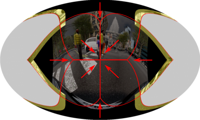
The most direct generalization of the shifting in the pixel grid of the original SWIN-transformer is a shifting in the HEALPix grid along the axes of the quadrilaterals of the base-resolution pixels, cf. Figure 4 (left). We call this grid shifting. Similarly to the original SWIN shifting scheme, there are boundary effects at the edge of the half sphere covered by the grid. Additionally, due to the alignment of the base pixels relative to each other, the shifting necessarily clashes at some base-pixel boundaries in the bulk of the image. As in the original SWIN transformer, both of these effects are handled by reshuffling the problematic pixels to fill up all windows and subsequently masking the attention mechanism to not attend to pixel pairs which originate from different regions of the sphere.

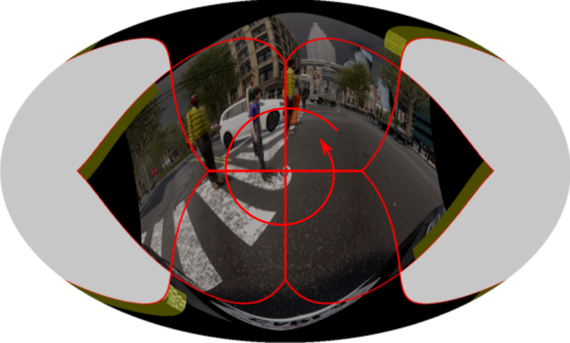
In the spiral shifting scheme, we first convert the nested ordering into a ring ordering and then perform a roll operation on that list. Finally, we convert back to the nested ordering. In this way, windows are shifted along the azimuthal angle, with slight distortions which grow larger towards the poles due to the decreased length of circles of constant latitude, cf. Figure 4 (right). As in the grid shifting scheme, we encounter boundary effects. In the spiral shifting, they occur at the pole and at the boundary of the half sphere covered by the grid. These effects are again handled by reshuffling the pixels and masking the attention mechanism appropriately. In this scheme, there are no boundary effects in the bulk of the image.

Both shifting strategies can be implemented as precomputed indexing operations on the list holding the HEALPix features and are therefore efficient. In ablation studies we found that the spiral shifting outperforms the grid shifting slightly.

3.4 Relative position bias

In the SWIN-transformer, an important component that adds spatial information is the relative position bias which is added to the query-key product in the attention layers. This bias is a learned value which depends only on the difference vector between the pixels in a pixel pair, i.e. all pixel pairs with the same relative position receive the same bias contribution.

In the HEALPix grid, the pixels inside each base quadrilateral are arranged in an approximately rectangular grid which we use to compute the relative positions of pixel pairs for obtaining the relative position bias mapping. We share the same relative position bias table across all windows, so in particular also across base quadrilaterals. We also experimented with an absolute position embedding after the patch embedding layer but observed no benefit for performance.

4 Experiments

To verify the performance of our model, we trained the HEAL-SWIN and the SWIN transformer on challenging realistic datasets of fisheye camera images from the autonomous driving domain. We show that our model reaches better predictions for semantic segmentation and depth estimation on both datasets we tried.

4.1 Datasets

Figure 5: Example from the Large+AD SynWoodScape dataset, projected onto the plane. Regions not covered by the $\nicefrac{{8}}{{12}}$ base pixels of the HEALPix grid are shown as hatched. The left panel shows the RGB image while the right panel shows the corresponding semantic segmentation ground truth. See Section 4.4 for more details.

We evaluate our models using the SynWoodScape [16] dataset of 2000 fisheye images from synthetic street scenes generated using the driving simulator CARLA [34] and the real-world WoodScape dataset [17] consisting of 8234 fisheye images recorded in various environments in the US, Europe and China. We use the pixel-wise classification labels contained in both datasets for semantic segmentation and the pixel-wise depth values in SynWoodScape for depth regression. For SynWoodScape, the ground truth labels are pixel-perfect and in particular provide dense depth maps, allowing for a clean comparison of model performances. For WoodScape however, we noticed inconsistencies in the semantic labels and no dense depth values are available. Further details can be found in Appendix A.

In both datasets, the images are presented as flat pixel grids together with calibration data which allows for a projection onto the sphere. In order to project the data to the HEALpix grid, we use the healpy [14] package to get the azimuthal and polar angles of the grid points inside the $\nicefrac{{8}}{{12}}$ base pixels which roughly cover half of the sphere. These angles are then projected to the plane using the calibration information and the data is resampled to the projected points. For the images, we use bilinear interpolation for the resampling, while the ground truths are resampled with a nearest neighbor interpolation.

Although using only eight out of the twelve base pixel of the HEALPix grid allows for an efficient representation of the fisheye images, some image pixels are projected to regions outside of the coverage of our subset of the HEALPix grid; see hatched regions in Figure 5. However, the affected pixels lie at the corners of the image, making the tradeoff well worth it for the autonomous driving tasks considered here. We restrict evaluation to the eight base pixels, as detailed in section 4.3 for depth estimation and section 4.4 for semantic segmentation.

For the SWIN transformer, we rescale the input images to a size of $640\times 768$, corresponding to around $492\mathrm{k}$ pixels, for HEAL-SWIN, we use $n_{\mathrm{side}}=256$, corresponding to roughly $525\mathrm{k}$ pixels.

4.2 Models

For both the depth estimation and the semantic segmentation task, we compare the performance of HEAL-SWIN on the HEALPix images to that of the SWIN transformer on the original, i.e. flat and distorted fisheye images. The architecture and training hyperparameters were fixed by ablation studies for semantic segmentation on WoodScape unless stated otherwise. Furthermore, we use the same SWIN and HEAL-SWIN models for both semantic segmentation and depth estimation, and change only the number of output channels in the final layer.

As a baseline, we use the SWIN transformer in a $12$-layer configuration similar to the “tiny” configuration SWIN-T from the original paper [15] with a patch size of $2\times 2$ and a window size of $8\times 8$, adapted to the size of our input images. Since both tasks require predictions of the same spatial dimensions as the input, we mirror the SWIN encoder in a SWIN decoder and add skip connections in a SWIN-UNet architecture [33], resulting in a model of around $41\mathrm{M}$ parameters. We found the improved layer-norm placement and cosine attention introduced in [32] to be very effective and use them in all our models.

For the HEAL-SWIN models, we use the same configurations as for the SWIN model with a (one-dimensional) patch size of $4$, mirroring the $2\times 2$ on the flat side and a window size of $64$, mirroring the $8\times 8$ on the flat side. For shifting, we use the spiral shifting introduced in Section 3.3 with a shift size of $4$, corresponding roughly to half windows. Again, we mirror the encoder and add skip connections to obtain a UNet-like architecture. Patch merging reduces the number of pixels by a factor of four leading to four windows per base pixel in the bottleneck. A table with the spatial feature dimensions throughout the network can be found in Appendix B. The shared model configuration gives our HEAL-SWIN model the same total parameter count as the SWIN model.

For the semantic segmentation task we train all models on four Nvidia A40 GPUs with an effective batch size of $8$ and a constant learning rate of about $9.4\times 10^{-4}$. For the depth estimation task we used an effective batch size of 4 and learning rates of $5\times 10^{-3}$ and $5\times 10^{-5}$ for the HEAL-SWIN and SWIN models respectively, chosen from the best performing models after a learning rate ablation.

4.3 Depth estimation

Figure 6: Depth-map ground truth for the image in Figure 5 (left) and corresponding point cloud (right). The red arrow indicates the orientation of the camera.

Estimating distances to obstacles and other road users is an important task for 3d scene understanding and route planning in autonomous driving. In depth estimation, pixel-wise distance maps are predicted from camera images. For the SynWoodScape dataset, pixel-perfect ground truth depth maps are available on which we train our models, adjusted to one output channel. The model is trained using an $L_{2}$ loss and the depth data is standardized to have zero mean and unit variance; in addition the sky is masked out during training and evaluation. In order to preserve the common high-contrast edges all resampling is done using nearest neighbor interpolation.

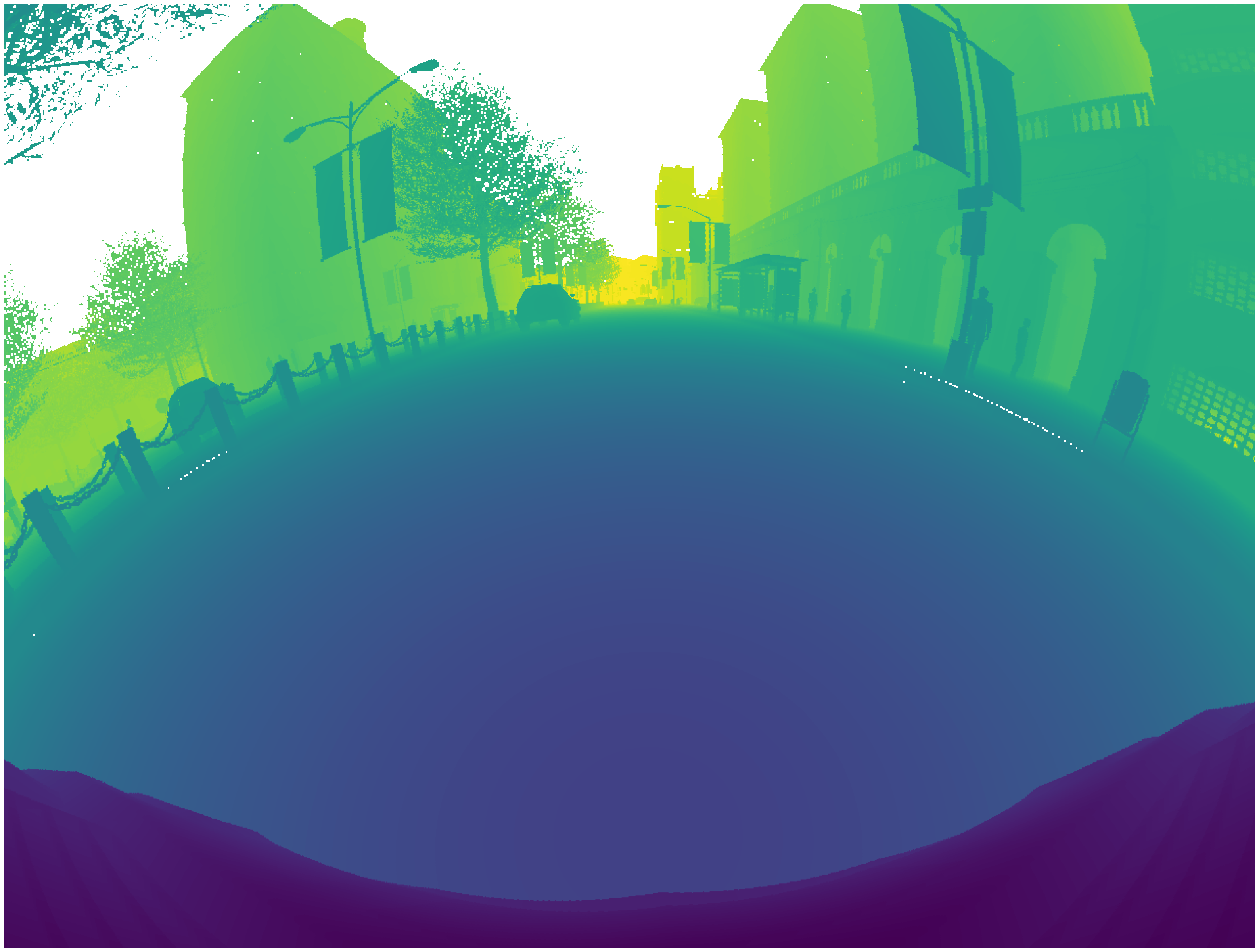
In order to capture the quality of 3D scene predictions of the different models, we evaluate the depth estimations in terms of point clouds. More specifically, we generate a point cloud from the ground truth depth values by computing azimuthal and polar angles for each pixel from the calibration information of the camera and scaling the corresponding vectors on the unit sphere with the depth values. An example of the resulting point cloud is displayed in Figure 6 (right). Similarly, the SWIN predictions are transformed into a point cloud, as are the HEAL-SWIN predictions, for which we use the pixel positions in HEALPix for the spherical angles. Comparing the predicted point clouds to the full-resolution ground truth point cloud leads to an evaluation scheme which is sensitive to the 3D information in the predicted depth values, which is essential for downstream tasks.

To compare the predicted point cloud $P_{\text{pred}}$ to the ground truth point cloud $P_{\text{gt}}$ in a symmetrical way, we use the Chamfer distance [35] defined by

$$\text{CD}(P_{\text{pred}},P_{\text{gt}})=\frac{1}{|P_{\text{pred}}|}\sum_{p\in P_{\text{pred}}}\min_{p^{\prime}\in P_{\text{gt}}}d(p,p^{\prime})^{2}+\frac{1}{|P_{\text{gt}}|}\sum_{p\in P_{\text{gt}}}\min_{p^{\prime}\in P_{\text{pred}}}d(p,p^{\prime})^{2}\,,$$

where $d(p,p^{\prime})$ is the Euclidean distance between $p$ and $p^{\prime}$. As mentioned in Section 4.1, some pixels in the corners of the image are lost when converted to the HEALPix grid. In order to ensure a fair comparison, we mask the pixels unavailable to the HEAL-SWIN model in the loss of the SWIN model and exclude them from $P_{\text{pred}}$ and $P_{\text{gt}}$.

The resulting depth estimation Chamfer distances are plotted in Figure 3. From this there is a clear signal that the point clouds predicted by HEAL-SWIN match the ground truth point cloud better than the point cloud predicted by the SWIN transformer, indicating that the HEAL-SWIN model has indeed learned a better 3D representation of the spherical images.

4.4 Semantic segmentation

Table 1: Mean intersection over union on the sphere for semantic segmentation with HEAL-SWIN and SWIN, averaged over three runs. For WoodScape, we exclude the void class from the mean but keep it in the loss.

Model	Dataset	mIoU
HEAL-SWIN	Large SynWoodScape	0.947
SWIN	Large SynWoodScape	0.918
HEAL-SWIN	Large+AD SynWoodScape	0.841
SWIN	Large+AD SynWoodScape	0.809
HEAL-SWIN	WoodScape	0.628
SWIN	WoodScape	0.617

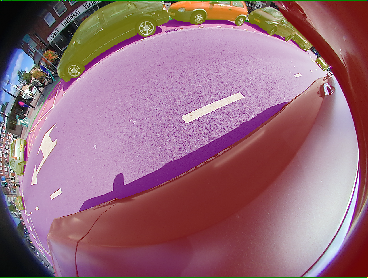
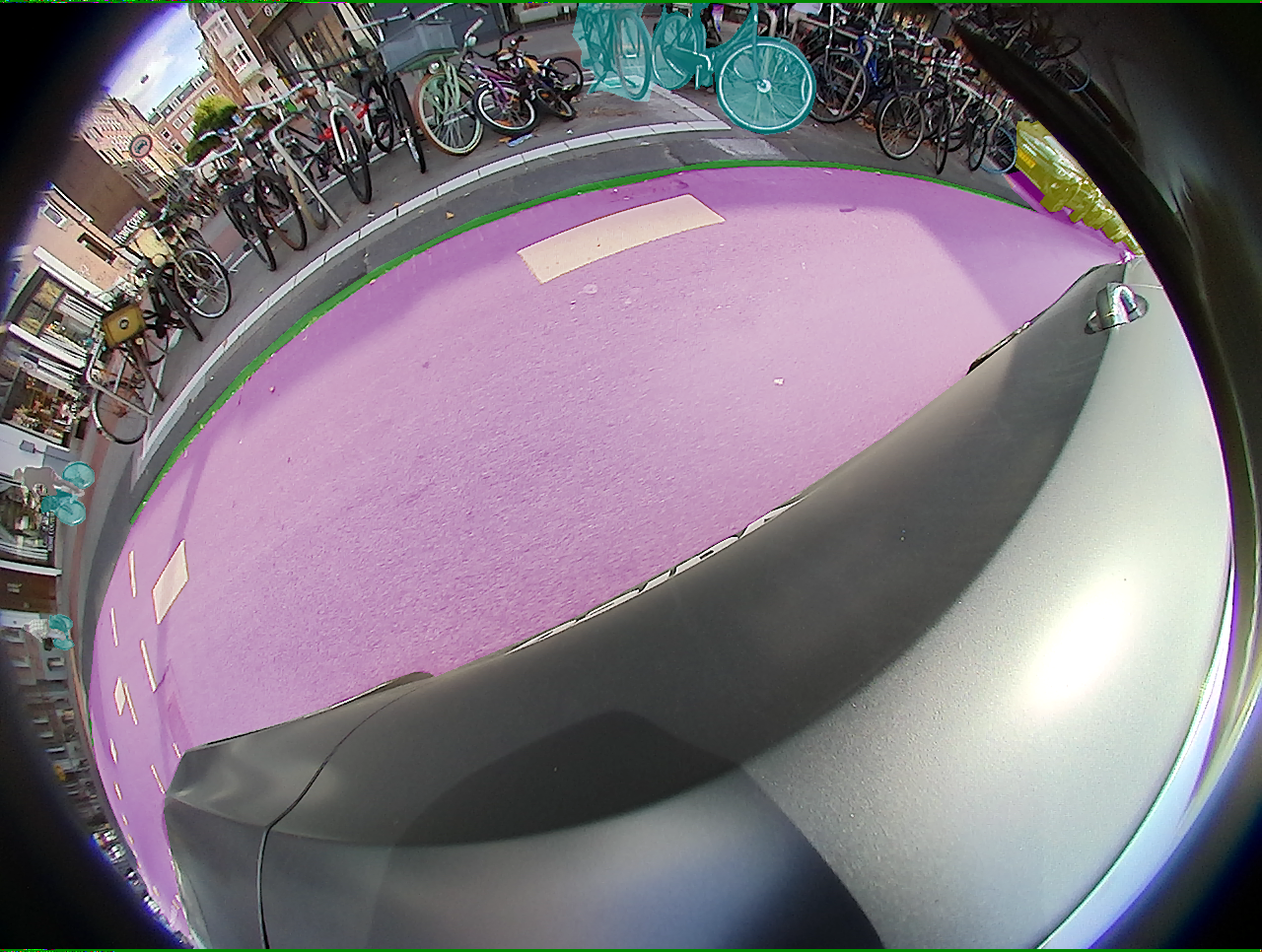
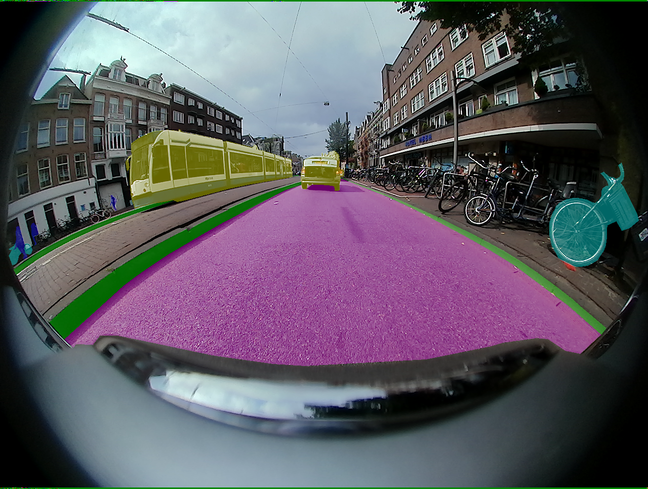
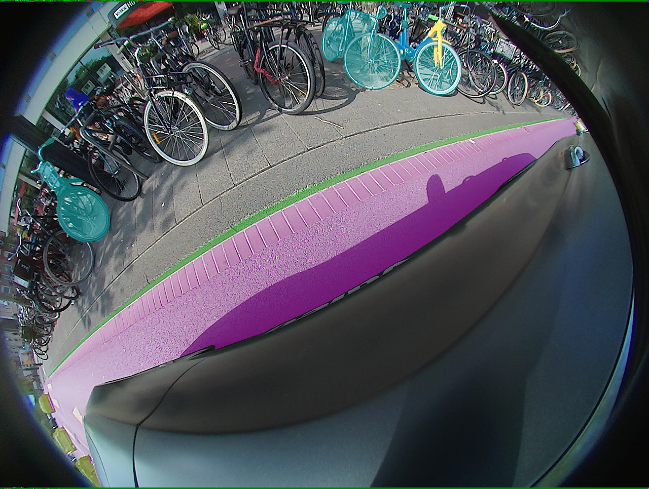
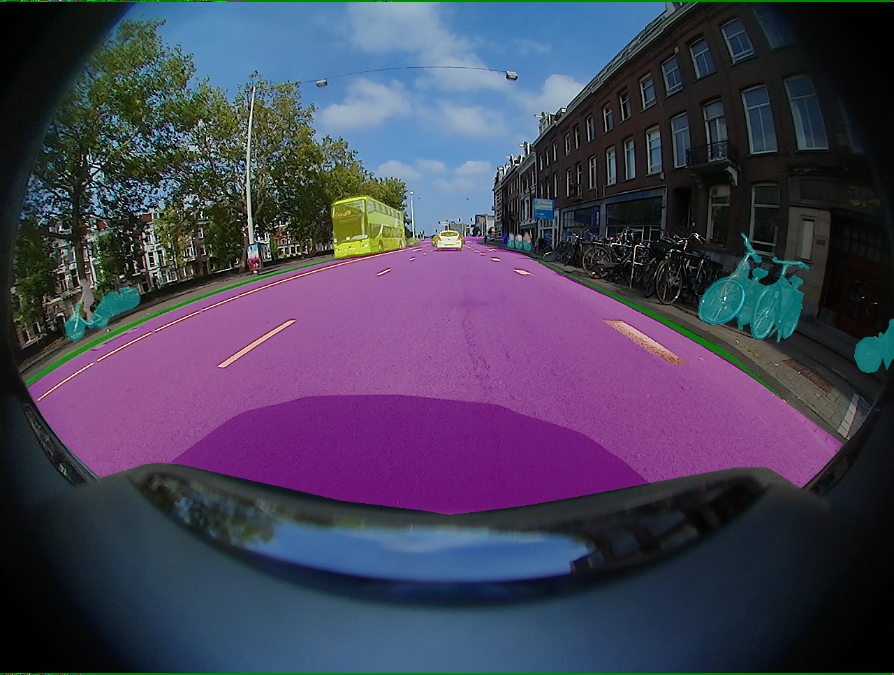
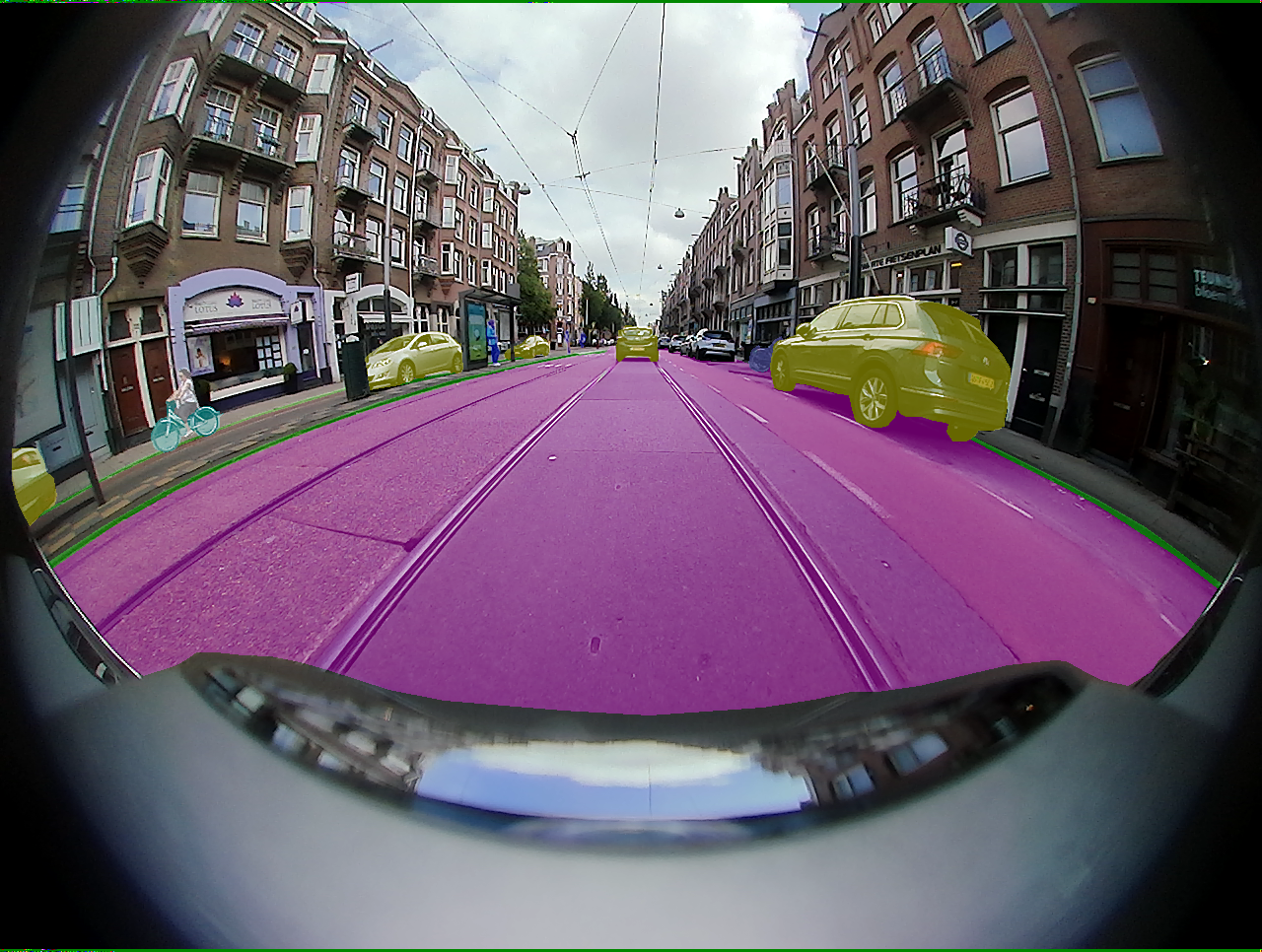
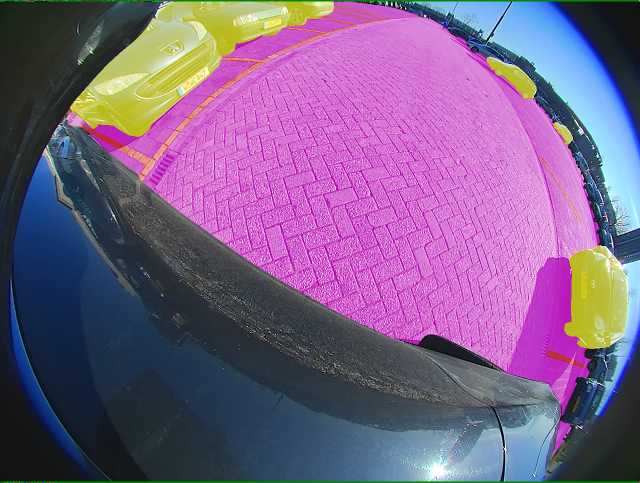
Semantic segmentation is a pixel-wise classification task for which we train HEAL-SWIN and SWIN on ground truth segmentation masks from WoodScape and SynWoodScape. For WoodScape, we train on the ten classes for which segmentation masks are directly available in the provided dataset. For SynWoodScape, we use two different subsets out of the 25 classes provided in the dataset. All excluded classes are mapped to void. In the first subset, which we call Large SynWoodScape, we train on 8 classes which cover large areas of the image, like building, ego-vehicle, road etc. obtaining a dataset which lacks a lot of fine details and hence minimizes projection effects between the flat projection and HEALPix. For the second subset, Large+AD SynWoodScape, we include further classes relevant to autonomous driving, like pedestrian, traffic light and traffic sign to create a more realistic dataset of 12 classes which also features finer details; see Figure 5 for a sample. Further details about the datasets can be found in Appendix A.

We adjust the number of output channels in the base HEAL-SWIN and SWIN models described in Section 4.2 to the number of classes and train with a weighted pixel-wise cross-entropy loss. We choose the class weights $w_{i}$ to be given in terms of the class prevalences $n_{i}$ by $w_{i}=n_{i}^{-1/4}$.

Figure 7: Semantic Segmentation for varying training set sizes. Performance is measured as the mean intersection over union (higher is better) computed on the HEALPix grid (spherical mIoU).

As we argued in the introduction, for downstream tasks like collision avoidance, spatial information, such as the angle relative to the driving direction under which a pedestrian is detected, is essential. This information is obtained from the segmentation mask on the sphere as directly predicted by HEAL-SWIN. As summarized in Table 1, the HEAL-SWIN predictions are considerably more accurate than the SWIN predictions projected onto the sphere. For reference, we also evaluated both models on the distorted segmentation masks on the flat grid, projecting the predicted HEAL-SWIN masks, as summarized in Appendix C. Note that on WoodScape, we compute the mIoU in a different way from the 2021 CVPR competition [36] to account for the flaws in the metric used there, as discussed in more detail in Appendix A. We clearly see that on the sphere, the HEAL-SWIN model performs best for all datasets, whereas SWIN loses a considerable amount of performance in the projection step onto the sphere.

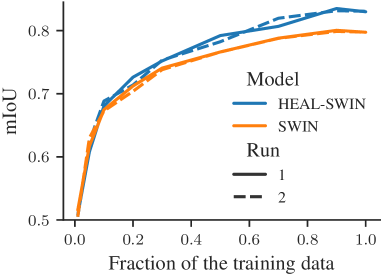
We also study the effects of the size of the dataset used in training. Since we have limited data, we simulate different data set sizes by using different subsets of the training data. We train on the SynWoodScape data with the Large+AD SynWoodScape class subset. Within a run, we use exactly the same subset for both models, HEAL-SWIN and SWIN, while strictly increasing the subset when moving to a larger training set. All models are trained entirely from scratch until convergence and evaluated using the entire validation set. We find that the HEAL-SWIN model can make better use of larger training sets than the SWIN model, as the difference in performance becomes larger the more training data is used as shown in Figure 7.

5 Conclusion

High-resolution spherical data is ubiquitous in application domains ranging from robotics to climate science. Safety-critical downstream tasks based on fisheye cameras, such as collision avoidance in autonomous driving, require precise 3D spatial information to be extracted from 2D spherical images, and we therefore proposed to incorporate the geometry without projection distortions by training with images directly on the sphere. To implement this idea, we constructed the efficient vision tranformer HEAL-SWIN, combining the HEALPix spherical grid with the SWIN transformer. We showed superior performance of our HEAL-SWIN model on the sphere, in comparison to a comparable SWIN model on flat images, for depth estimation and semantic segmentation on automotive fisheye images.

Although showing high performance already in its present form, HEAL-SWIN still has ample room for improvement. Firstly, in the presented setup, the grid is cut along base pixels to cover half of the sphere, leaving parts of the image uncovered while parts of the grid are unused. This could be improved by descending with the boundary into the nested structure of the grid and adapting the shifting strategy accordingly. Secondly, the relative position bias currently does not take into account the different base pixels around the poles and around the equator. This could be solved by a suitable correction deduced from the grid structure. Thirdly, the UNet-like architecture we base our setup on, is not state-of-the-art in tasks like semantic segmentation. Adapting a modern vision transformer decoder head to HEALPix could boost performance even further. Finally, our setup is not yet equivariant with respect to rotations of the sphere. For equivariant tasks like semantic segmentation or depth estimation, a considerable performance boost can be expected from making the model equivariant [37]. In this context it would also be very interesting to investigate equivariance with respect to local transformations. This has been thoroughly analyzed for CNNs in [38, 39, 40] and a gauge equivariant transformer has been proposed in [41].

Appendix to
HEAL-SWIN: A Vision Transformer On The Sphere

In this appendix to the article “HEAL-SWIN: A Vision Transformer On The Sphere”, we provide further details about the datasets and models used in the experimental section.

Appendix A Datasets

For our experiments we use the WoodScape [17] and the SynWoodScape [16] dataset. Note that we used the 2k samples which were published at https://drive.google.com/drive/folders/1N5rrySiw1uh9kLeBuOblMbXJ09YsqO7I at the time of writing, instead of the full 80k samples. In all experiments, we split the available samples randomly (but consistently across models and runs) into 80% training data and 20% validation data.

For the semantic segmentation task, we use the 10 classes for which semantic masks are provided in the WoodScape dataset and two different subsets of the 25 classes for the SynWoodScape dataset. Table 2 shows the relation between the 25 original classes and the classes in our two subsets. See Figure 8 for the class prevalences in the different datasets. Examples for the inconsistent semantic masks in the WoodScape dataset mentioned in the main text can be found in Figure 9.

Table 2: Classes from the Large SynWoodScape and the Large+AD SynWoodScape datasets in terms of the classes provided by SynWoodScape.

SynWoodScape	Our Classes
	Large SynWoodScape	Large+AD SynWoodScape
unlabeled	void	void
building	building	building
fence	void	void
other	void	void
pedestrian	void	pedestrian
pole	void	void
road line	road line	road line
road	road	road
sidewalk	sidewalk	sidewalk
vegetation	void	void
four-wheeler vehicle	four-wheeler vehicle	four-wheeler vehicle
wall	void	void
traffic sign	void	traffic sign
sky	sky	sky
ground	void	void
bridge	void	void
rail track	void	void
guard rail	void	void
traffic light	void	traffic light
water	void	void
terrain	void	void
two-wheeler vehicle	void	two-wheeler vehicle
static	void	void
dynamic	void	void
ego-vehicle	ego-vehicle	ego-vehicle

In the 2021 CVPR competition for segmentation of the WoodScape dataset [36], pixels which are labeled with the dominant void class in the ground truth were excluded from the mIoU used for ranking. Therefore, many teams excluded the void class from their training loss, resulting in random predictions for large parts of the image. This shortcoming was noted in [36], but the evaluation score could not be changed after the competition had been published. Given these circumstances, we decided to include the void class into our training loss but exclude it from the mean over classes in the mIoU to more accurately reflect the performance of our models on the more difficult classes. However, this also means that our results cannot be directly compared to the results of the competition.

The same problem does not arise for the SynWoodScape dataset and our two variants since their class lists include all major structures in the image, leading to a much reduced prevalence of the void class. Therefore, we include all classes in the mIoU for these datasets.

Figure 8: Class distributions for the datasets used in semantic segmentation.

(a) Large parts of the ego vehicle are labeled as lanemarks.

(b) Some (but not all) parked bicycles are labeled as bicycle.

(c) Some (but not all) parked cars are labeled as vehicles.

Figure 9: Examples of inconsistencies in semantic masks of the WoodScape dataset.

Appendix B SWIN and HEAL-SWIN models

In Table 3 we provide further details on the spatial size of the features throughout the HEAL-SWIN model used in the experiments discussed in Section 4.

Table 3: Spatial features per layer in the HEAL-SWIN models used for the experiments described in Section 4.

layer	pixel / patches	windows	windows per base pixel	$n_{\mathrm{side}}$	followed by
input	524288	8192	1024	256	patch embedding
HEAL-SWIN block 1	131072	2048	256	128	patch merging
HEAL-SWIN block 2	32768	512	64	64	patch merging
HEAL-SWIN block 3	8192	128	16	32	patch merging
HEAL-SWIN block 4	2048	32	4	16	patch expansion
HEAL-SWIN block 5	8192	128	16	32	patch expansion
HEAL-SWIN block 6	32768	512	64	64	patch expansion
HEAL-SWIN block 7	131072	2048	256	128	patch expansion
output	524288	8192	1024	256	—

Appendix C HEAL-SWIN versus SWIN for flat segmentation

In Table 4, we show the results of evaluating the segmentation models discussed in Section 4.4 on the plane. In this case, the HEAL-SWIN predictions are projected onto the pixel grid of the SWIN predictions before evaluation. To ensure a fair comparison, the flat mIoU is calculated on a masked region of this grid, removing pixels which lie outside of the (restricted) HEALPix grid we use.

Table 4: Mean IoU for semantic segmentation with HEAL-SWIN and SWIN, averaged over three runs, after projection onto the plane. For WoodScape, we exclude the void class from the mean but keep it in the loss.

Model	Dataset	flat mIoU
HEAL-SWIN	Large SynWoodScape	0.899
SWIN	Large SynWoodScape	0.930
HEAL-SWIN	Large+AD SynWoodScape	0.790
SWIN	Large+AD SynWoodScape	0.837
HEAL-SWIN	WoodScape	0.611
SWIN	WoodScape	0.620

References

- [1] Y. Qian, M. Yang, and J. M. Dolan, “Survey on fish-eye cameras and their applications in intelligent vehicles,” IEEE Transactions on Intelligent Transportation Systems 23 (2022) 22755–22771.
- [2] C. Zhang, S. Liwicki, W. Smith, and R. Cipolla, “Orientation-aware semantic segmentation on Icosahedron spheres,” in Proceedings of the IEEE/CVF International Conference on Computer Vision (ICCV), pp. 3532–3540. IEEE, 2019. arXiv:1907.12849.
- [3] Y. Lee, J. Jeong, J. Yun, W. Cho, and K.-J. Yoon, “SpherePHD: Applying CNNs on a spherical PolyHeDron representation of 360 degree images,” arXiv:1811.08196.
- [4] N. Haim, N. Segol, H. Ben-Hamu, H. Maron, and Y. Lipman, “Surface Networks via general covers,” in Proceedings of the IEEE/CVF International Conference on Computer Vision (ICCV), pp. 632–641. IEEE, 2019. arXiv:1812.10705.
- [5] M. Eder and J.-M. Frahm, “Convolutions on spherical images,” in Proceedings of the IEEE/CVF Conference on Computer Vision and Pattern Recognition (CVPR) Workshops, pp. 1–5. IEEE, 2019. arXiv:1905.08409.
- [6] H. Du, H. Cao, S. Cai, J. Yan, and S. Zhang, “Spherical Transformer: Adapting spherical signal to CNNs,” arXiv:2101.03848.
- [7] M. Shakerinava and S. Ravanbakhsh, “Equivariant networks for pixelized spheres,” in Proceedings of the 38th International Conference on Machine Learning (ICML), pp. 9477–9488. PMLR, 2021. arXiv:2106.06662.
- [8] K. Tateno, N. Navab, and F. Tombari, “Distortion-aware convolutional filters for dense prediction in panoramic images,” in Computer Vision – ECCV 2018, V. Ferrari, M. Hebert, C. Sminchisescu, and Y. Weiss, eds., vol. 11220 of Lecture Notes in Computer Science, pp. 732–750. Springer International Publishing, 2018.
- [9] T. S. Cohen, M. Geiger, J. Köhler, and M. Welling, “Spherical CNNs,” in Proceedings of the International Conference on Learning Representations (ICLR). 2018. arXiv:1801.10130.
- [10] C. Esteves, A. Makadia, and K. Daniilidis, “Spin-weighted spherical CNNs,” in Advances in Neural Information Processing Systems, vol. 33, pp. 8614–8625. Curran Associates Inc., 2020. arXiv:2006.10731.
- [11] O. Cobb, C. G. R. Wallis, A. N. Mavor-Parker, A. Marignier, M. A. Price, M. d’Avezac, and J. McEwen, “Efficient generalized spherical CNNs,” in Proceedings of the International Conference on Learning Representations (ICLR). 2021. arXiv:2010.11661.
- [12] J. R. Driscoll and D. M. Healy, “Computing Fourier transforms and convolutions on the 2-sphere,” Advances in Applied Mathematics 15 (1994) 202–250.
- [13] K. M. Gorski, E. Hivon, and B. D. Wandelt, “Analysis issues for large CMB data sets,” arXiv:astro-ph/9812350.
- [14] A. Zonca, L. Singer, D. Lenz, M. Reinecke, C. Rosset, E. Hivon, and K. Gorski, “healpy: equal area pixelization and spherical harmonics transforms for data on the sphere in Python,” Journal of Open Source Software 4 (2019) 1298.
- [15] Z. Liu, Y. Lin, Y. Cao, H. Hu, Y. Wei, Z. Zhang, S. Lin, and B. Guo, “Swin transformer: Hierarchical vision transformer using shifted windows,” in Proceedings of the IEEE/CVF International Conference on Computer Vision (ICCV), pp. 9992–10002. IEEE, 2021. arXiv:2103.14030.
- [16] A. R. Sekkat, Y. Dupuis, V. R. Kumar, H. Rashed, S. Yogamani, P. Vasseur, and P. Honeine, “SynWoodScape: Synthetic surround-view fisheye camera dataset for autonomous driving,” IEEE Robotics and Automation Letters 7 (2022) 8502–8509, arXiv:2203.05056.
- [17] S. Yogamani, C. Hughes, J. Horgan, G. Sistu, S. Chennupati, M. Uricar, S. Milz, M. Simon, K. Amende, C. Witt, H. Rashed, S. Nayak, S. Mansoor, P. Varley, X. Perrotton, D. Odea, and P. Perez, “Woodscape: A multi-task, multi-camera fisheye dataset for autonomous driving,” in Proceedings of the IEEE/CVF International Conference on Computer Vision (ICCV), pp. 9307–9317. IEEE, 2019. arXiv:1905.01489.
- [18] A. Vaswani, N. Shazeer, N. Parmar, J. Uszkoreit, L. Jones, A. N. Gomez, and Łukasz Kaiser, “Attention is all you need,” in Advances in Neural Information Processing Systems, vol. 30. Curran Associates, Inc., 2017. arXiv:1706.03762.
- [19] A. Dosovitskiy, L. Beyer, A. Kolesnikov, D. Weissenborn, X. Zhai, T. Unterthiner, M. Dehghani, M. Minderer, G. Heigold, S. Gelly, J. Uszkoreit, and N. Houlsby, “An image is woth 16x16 words: Transformers for image recognition at scale,” in Proceedings of the International Conference on Learning Representations (ICLR). 2021. arXiv:2010.11929.
- [20] S. Cho, R. Jung, and J. Kwon, “Spherical transformer,” arXiv:2202.04942.
- [21] S. R. Cachay, P. Mitra, H. Hirasawa, S. Kim, S. Hazarika, D. Hingmire, P. Rasch, H. Singh, and K. Ramea, “Climformer – a spherical transformer model for long-term climate projections,” in Proceedings of the Machine Learning and the Physical Sciences Workshop, NeurIPS 2022. 2022.
- [22] J. Guibas, M. Mardani, Z. Li, A. Tao, A. Aanandkumar, and B. Catanzaro, “Adaptive Fourier neural operators: Efficient token mixers for transformers,” in Proceedings of the International Conference on Learning Representations (ICLR). 2022. arXiv:2111.13587.
- [23] J. Mao, Y. Xue, M. Niu, H. Bai, J. Feng, X. Liang, H. Xu, and C. Xu, “Voxel transformer for 3d object detection,” in Proceedings of the IEEE/CVF International Conference on Computer Vision (ICCV), pp. 3144–3153. IEEE, 2021. arXiv:2109.02497.
- [24] L. Fan, Z. Pang, T. Zhang, Y.-X. Wang, H. Zhao, F. Wang, N. Wang, and Z. Zhang, “Embracing single stride 3d object detector with sparse transformer,” in Proceedings of the IEEE/CVF Conference on Computer Vision and Pattern Recognition (CVPR), pp. 8448–8458. IEEE, 2022. arXiv:2112.06375.
- [25] X. Lai, J. Liu, L. Jiang, L. Wang, H. Zhao, S. Liu, X. Qi, and J. Jia, “Stratified transformer for 3d point cloud segmentation,” in 2022 IEEE/CVF Conference on Computer Vision and Pattern Recognition (CVPR), pp. 8490–8499. IEEE, 2022. arXiv:2203.14508.
- [26] X. Lai, Y. Chen, F. Lu, J. Liu, and J. Jia, “Spherical transformer for LiDAR-based 3d recognition,” arXiv:2303.12766.
- [27] X. Guo, Y. Sun, R. Zhao, L. Kuang, and X. Han, “SWPT: Spherical window-based point cloud transformer,” in Computer Vision – ACCV 2022. ACCV 2022, L. Wang, J. Gall, T. J. Chin, I. Sato, and R. Chellappa, eds., vol. 13841 of Lecture Notes in Computer Science, pp. 396–412. Springer International Publishing, 2023.
- [28] Krachmalnicoff, N. and Tomasi, M., “Convolutional neural networks on the HEALPix sphere: A pixel-based algorithm and its application to CMB data analysis,” A&A 628 (2019) A129, arXiv:1902.04083.
- [29] N. Perraudin, M. Defferrard, T. Kacprzak, and R. Sgier, “DeepSphere: Efficient spherical convolutional neural network with HEALPix sampling for cosmological applications,” Astronomy and Computing 27 (2019) 130–146, arXiv:1810.12186.
- [30] M. Defferrard, M. Milani, F. Gusset, and N. Perraudin, “DeepSphere: A graph-based spherical CNN,” in Proceedings of the International Conference on Learning Representations (ICLR). 2020. arXiv:2012.15000.
- [31] C. Jiang, J. Huang, K. Kashinath, Prabhat, P. Marcus, and M. Nießner, “Spherical CNNs on unstructured grids,” in Proceedings of the International Conference of Learning Representations (ICLR). 2019. arXiv:1901.02039.
- [32] Z. Liu, H. Hu, Y. Lin, Z. Yao, Z. Xie, Y. Wei, J. Ning, Y. Cao, Z. Zhang, L. Dong, F. Wei, and B. Guo, “Swin transformer v2: Scaling up capacity and resolution,” in Proceedings of the IEEE/CVF International Conference on Computer Vision and Pattern Recognition (CVPR), pp. 11999–12009. IEEE, 2022. arXiv:2111.09883.
- [33] H. Cao, Y. Wang, J. Chen, D. Jiang, X. Zhang, Q. Tian, and M. Wang, “Swin-Unet: Unet-like pure transformer for medical image segmentation,” in Computer Vision – ECCV 2022 Workshops. ECCV 2022, L. Karlinsky, T. Michaeli, and K. Nishino, eds., vol. 13803 of Lecture Notes in Computer Science, pp. 205–218. Springer International Publishing, 2022. arXiv:2105.05537.
- [34] A. Dosovitskiy, G. Ros, F. Codevilla, A. Lopez, and V. Koltun, “CARLA: An open urban driving simulator,” in Proceedings of the 1st Annual Conference on Robot Learning, pp. 1–16. 2017.
- [35] H. Barrow and J. Tenenbaum, “Parametric correspondence and chamfer matching: Two new techniques for image matching,” in Proceedings of the International Joint Conferences on Artificial Intelligence (IJCAI), vol. 2, pp. 659–670. MIT, 1977.
- [36] S. Ramachandran, G. Sistu, J. McDonald, and S. Yogamani, “Woodscape Fisheye Semantic Segmentation for Autonomous Driving – CVPR 2021 OmniCV Workshop Challenge,” arXiv:2107.08246.
- [37] J. E. Gerken, O. Carlsson, H. Linander, F. Ohlsson, C. Petersson, and D. Persson, “Equivariance versus augmentation for spherical images,” in Proceedings of the International Conference on Machine Learning (ICML), pp. 7404–7421. PMLR, 2022. arXiv:2202.03990.
- [38] T. Cohen, M. Weiler, B. Kicanaoglu, and M. Welling, “Gauge equivariant convolutional networks and the Icosahedral CNN,” in Proceedings of the International Conference on Machine learning (ICML), pp. 1321–1330, PMLR. 2019. arXiv:1902.04615.
- [39] M. C. Cheng, V. Anagiannis, M. Weiler, P. de Haan, T. S. Cohen, and M. Welling, “Covariance in physics and convolutional neural networks,” arXiv:1906.02481.
- [40] J. E. Gerken, J. Aronsson, O. Carlsson, H. Linander, F. Ohlsson, C. Petersson, and D. Persson, “Geometric deep learning and equivariant neural networks,” arXiv:2105.13926.
- [41] L. He, Y. Dong, Y. Wang, D. Tao, and Z. Lin, “Gauge equivariant transformer,” in Neural Information Processing Systems, vol. 34, pp. 27331–27343. Curran Associates, Inc., 2021.