Attainable bounds for algebraic connectivity and maximally-connected regular graphs

Abstract

We derive attainable upper bounds on the algebraic connectivity (spectral gap) of a regular graph in terms of its diameter and girth. This bound agrees with the well-known Alon-Boppana-Friedman bound for graphs of even diameter, but is an improvement for graphs of odd diameter. For the girth bound, we show that only Moore graphs can attain it, and these only exist for very few possible girths. For diameter bound, we use a combination of stochastic algorithms and exhaustive search to find graphs which attain it. For 3-regular graphs, we find attainable graphs for all diameters $D$ up to and including $D=9$ (the case of $D=10$ is open). These graphs are extremely rare and also have high girth; for example we found exactly 45 distinct cubic graphs on 44 vertices attaining the upper bound when $D=7$; all have girth 8 (out of a total of about $10^{20}$ cubic graphs on 44 vertices, including 266362 having girth 8). We also exhibit families of $d$-regular graphs attaining upper bounds with $D=3$ and $4$, and with $g=6.$ Several conjectures are proposed.

1 Introduction

The Algebraic Connectivity of a graph (AC; also called the spectral gap) is an important measure of how well information propagates through the graph [1, 2], and corresponds to the second eigenvalue of the graph Laplacian matrix. The higher the AC, the better the graph is at diffusing information [3, 4, 5]. Graphs with high algebraic connectivity are related to expander graphs, and are important in many applications [6, 7]. This paper is motivated by the following question.

Problem 1.1

Find graphs which have the highest possible AC among all regular graphs of a given degree d and diameter $D,$ girth $g,$ or number of nodes $n.$

There are numerous works addressing this and related questions. A well known upper bound for AC in terms of diameter is the so-called Alon-Boppana-Friedman bound – see [8, 9, 10, 6]. Papers [11, 12, 13, 14] consider the question of maximizing AC over some families of possible graphs with a fixed number of vertices and edges. In paper [15] AC is maximized subject to a fixed diameter and number of edges. Papers [5, 16, 17] propose graph-growing algorithms to generate a high-AC graph on a large network with a given number of edges and vertices. Paper [18] considers maximizing AC for several families of random regular graphs. A complimentary question is explored in [19, 20], which asks what is the largest $n$ for a given AC and degree $d$.

In this work, we explore question 1.1 for a fixed girth or diameter. For even diameter, [8] gives a tight upper bound which – as we will see in §3 – is attained in many cases. In theorem 1.2 below, we will also derive the analogous tight bound for odd diameter, as well as for odd and even girths.

Theorem 1.2

Suppose that a $d-$regular graph has girth $g$ and diameter $D$ and let $AC$ be its algebraic connectivity. Then

$$AC\leq d-2(d-1)^{1/2}\cos\theta$$ (1)

where $\theta$ can be two of the following values.

• If $D$ is even with $D=2K,$ then $\theta$ is the smallest positive root of

  $$\tan(\theta K)=-\frac{d}{d-2}\tan\theta.$$ (2)

• If $D$ is odd with $D=2K-1,$ then $\theta$ be the smallest positive root of

  $$\tan(\theta K)=-\frac{\left(2\sqrt{d-1}\cos\theta+d\right)\sin\theta}{\sqrt{d-1}\left(d-2\cos^{2}\theta\right)+\left(d-2\right)\cos\theta}.$$ (3)

• If $g$ is even with $g=2K,$ then $\theta=\pi/K.$

• If $g$ is odd with $g=2K+1,$ then $\theta$ be the smallest root of

  $$\tan\left(\theta K\right)=-\frac{\sin\theta}{\left(d-1\right)^{-1/2}+\cos\theta}.$$ (4)

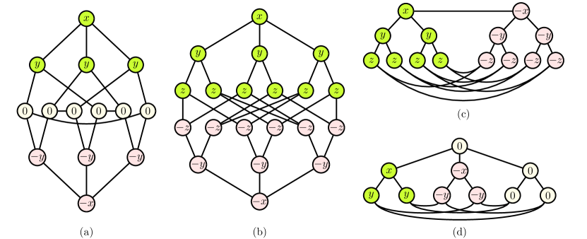
Figure 1: Some maximal cubic graphs and the form of the eigenvector corresponding to the second eigenvalue $\lambda_{2}$ of Laplacian. (a) Diameter-maximal graph “Crossing number 3H” [21] with D=4, AC=1.2679. (b) Diameter-maximal graph “Cubic integral G10” [22] with D=5, AC=1. (c) Girth-maximal graph with $g=6$, which is the Heawood graph having AC=1.585. (d) Girth-maximal graph with $g=5$, which is the Petersen graph having AC=2.

Upper bound for AC in terms of girth

3 4 5 6 7 8 9 10 11

3 4.0000 5.0000 6.0000 7.0000 8.0000 9.0000 10.000 11.000 12.000

4 3.0000 4.0000 5.0000 6.0000 7.0000 8.0000 9.0000 10.000 11.000

5 2.0000 2.6972 3.4384 4.2087 5.0000 5.8074 6.6277 7.4586 8.2984

6 1.5858 2.2679 3.0000 3.7639 4.5505 5.3542 6.1716 7.0000 7.8377

7 1.1864 1.7466 2.3738 3.0443 3.7458 4.4709 5.2147 5.9739 6.7460

8 1.0000 1.5505 2.1716 2.8377 3.5359 4.2583 5.0000 5.7574 6.5279

9 0.8088 1.3004 1.8706 2.4913 3.1481 3.8322 4.5380 5.2616 6.0000

10 0.7118 1.1975 1.7639 2.3820 3.0366 3.7191 4.4235 5.1459 5.8833

11 0.6069 1.0600 1.5983 2.1912 2.8229 3.4840 4.1685 4.8721 5.5916

12 0.5505 1.0000 1.5359 2.1270 2.7574 3.4174 4.1010 4.8038 5.5228

13 0.4872 0.9168 1.4356 2.0114 2.6277 3.2748 3.9462 4.6376 5.3456

Upper bound for AC in terms of diameter

3 4 5 6 7 8 9 10 11

3 2.0000 3.0000 4.0000 5.0000 6.0000 7.0000 8.0000 9.0000 10.000

4 1.2679 2.0000 2.7639 3.5505 4.3542 5.1716 6.0000 6.8377 7.6834

5 1.0000 1.6972 2.4384 3.2087 4.0000 4.8074 5.6277 6.4586 7.2984

6 0.7639 1.3542 2.0000 2.6834 3.3944 4.1270 4.8769 5.6411 6.4174

7 0.6571 1.2266 1.8587 2.5321 3.2356 3.9621 4.7070 5.4671 6.2398

8 0.5505 1.0665 1.6508 2.2810 2.9446 3.6340 4.3440 5.0709 5.8123

9 0.4965 1.0000 1.5762 2.2006 2.8597 3.5456 4.2527 4.9772 5.7164

10 0.4384 0.9111 1.4601 2.0598 2.6964 3.3613 4.0487 4.7546 5.4762

11 0.4069 0.8717 1.4156 2.0118 2.6456 3.3083 3.9939 4.6984 5.4187

12 0.3714 0.8167 1.3436 1.9245 2.5444 3.1941 3.8677 4.5607 5.2701

13 0.3512 0.7912 1.3148 1.8934 2.5115 3.1599 3.8323 4.5243 5.2329

Table 1: Upper bounds for AC in terms of girth and diameter. Known attainable bounds are in bold. Known unattainable are in italics. The rest are unknown.

The derivation of this theorem is given in §2. For even diameter, the bound (2) was already obtained in [8] (see Proposition 3.2 there; equation (2) is equivalent to formula for $\theta$ in Corollary 3.6 of [8]). For odd diameter, formula (3) is an improvement to the current literature as far as we are aware. The tight upper bound $\theta=\pi/K$ for even girth was previously derived in [14] in the context of cubic graphs. The bound for odd girth was given in [23].

For $g,G\leq 6$ and arbitrary $d,$ we have the following explicit formulas upper bounds:

$$D$$ upper bound

3

4

5

6

            

upper bound

3

4

5

6

It is easy to see that in all four cases of Theorem 1.2, $\frac{\pi}{2K}<\theta<\frac{\pi}{K}$, and $\theta\rightarrow\frac{\pi}{K}$ as $K\rightarrow\infty.$ The bound $\theta=\pi/K$ was also derived by Nilli [10], and both asymptote to the the Alon-Boppana estimate [24, 8] of $AC\sim d-2\sqrt{d-1}$ for random regular graphs as $D\rightarrow\infty$.

Table 1 lists the upper bounds for small $d,g,D$, and summarizes known attainable bounds. Many of these bounds are attainable, particularly with respect to diameter. Let us define a graph to be diameter-maximal or girth-maximal if it attains diameter (resp. girth) bound of theorem 1.2 (we will abbreviate it to “maximal” when prefix is understood from the context). Sections 3 and 4 of this paper are dedicated to a search for maximal graphs.

To illustrate where these bounds come from, consider the graph in figure 1(a). An eigenvector assigns a number to each vertex. Here, we take a specific eigenvector whose entries have values of $\pm x,\pm y,0$ associated to vertices as shown in the figure. This choice guarantees that the sum of the entries in the eigenvector is zero, and as such it is orthogonal to the $\left[1,1,\ldots,1\right]^{T}$ eigenvector corresponding to the zero eigenvalue of the Laplacian. Moreover both top and bottom vertices yield $\lambda x=3x-3y;$ whereas vertices at 2nd and 4th rows both read $\lambda y=3y-x.$ Correspondingly, the Laplacian matrix includes the spectrum of the matrix $\left[\begin{array}[c]{rr}3&-3\\ -1&3\end{array}\right].$ The smallest eigenvalue of this matrix is $1.2679,$ which is the upper bound for the AC of cubic graphs of diameter 4; a bound that is in fact attained by this graph.

Similarly, vertex assignment in (b), (c) and (d) yields matrices

$$\left[\begin{array}[c]{rrr}3&-3&0\\ -1&3&-2\\ 0&-1&5\end{array}\right],\ \left[\begin{array}[c]{rrr}4&-2&0\\ -1&3&-2\\ 0&-1&5\end{array}\right],\ \text{and\ }\left[\begin{array}[c]{rr}3&-2\\ -1&5\end{array}\right]$$

respectively, whose smallest eigenvalues (and upper bounds for AC) are $1,\ 1.5858,$ and$\ 2,$ respectively. In fact, these numbers are exactly the AC for these graphs.

Naturally most graphs don’t have such a nice structure. Nonetheless we show in §2 that these bounds hold for all graphs. For maximal graphs with odd diameter or odd/even girth, the proof also yields the exact number of vertices needed (the case of even diameter is more complicated). For example, figure 1(b) shows a maximal diameter-5 cubic graph with $n=20$ vertices. More generally, when $D=2K-1$ is odd, any maximal graph must contain exactly two Moore trees with $K$ levels. Girth-maximal graphs must consist entirely of the corresponding Moore trees (rooted at a vertex for odd girth, or at an edge for an even girth) along with additional edges joining the leafs. Correspondingly, maximal-girth graphs can only be attained by Moore graphs. This puts a severe restriction on the possible girth-maximal graphs. We summarize this as follows.

Theorem 1.3

Suppose that a diameter-maximal graph has an odd diameter, $D=2K-1.$ Then it is bipartite, and consists of two disjoint Bethe trees of $K$ levels with an additional $d\left(d-1\right)^{K-1}$ edges joining their leafs. It has exactly

$$n=2\left(1+d\sum_{j=0}^{K-2}\left(d-1\right)^{j}\right)=2\left(\frac{d\left(d-1\right)^{K-1}-2}{d-2}\right)$$ (5)

vertices.

Theorem 1.4

A girth-maximal graph must be a Moore graph, that is, a graph that attains a Moore bound for the number of vertices.

The situation is more complicated for even diameter $D=2K.$ In this case, a maximal graph consists of two Bethe trees with $K$ levels, plus a middle layer that is not part of either tree (see figure 1(a)). Each Bethe tree has $d-1$ edges going from each of its $d\left(d-1\right)^{K-2}$ leafs to the middle layer, for a total of $2d\left(d-1\right)^{K-1}$ edges going into the middle layer. This requires a minimum of $2\left(d-1\right)^{K-1}$ of vertices in the middle layer. We summarize:

Theorem 1.5

Suppose that a diameter-maximal graph has an even diameter, $D=2K.$ Then it consists of two disjoint Bethe trees of $K$ levels, plus a center of at least $\left(d-1\right)^{K-1}$ vertices that is not part of either trees. The total number of vertices $n$ satisfies

$$n\geq 2\left(1+d\sum_{j=0}^{K-2}\left(d-1\right)^{j}\right)+2\left(d-1\right)^{K-1}=4\left(\frac{\left(d-1\right)^{K}-1}{d-2}\right).$$

This lower bound on $n$ is sometimes attained and sometimes not. For example,when $d=3,D=4$, the lower bound $n=12$ is not attained (the smallest such maximal graph has 14 vertices, see §3.2). On the other hand, the lower bound is $n=16$ when $d=4,D=4,$ and it is attained by six distinct graphs (see §3.9).

Unlike odd diameter, we do not have a tight upper bound on $n$ for maximal graphs with even diameter. Asides from the obvious Moore bound, a nontrivial upper bound is given in [20]. For example consider the case of $d=3,D=4$, for which Theorem 1.2 gives $\max AC\approx 1.2679.$ Applying Theorem 8 from [20] with $r=3,t=5$ and $c=4.1$ yields $M\approx 27.8$ and therefore an upper bound of $n\leq 26,$ which is the best possible bound that can be obtained from Theorem 8 of [20] for this case. On the other hand, the biggest maximal graph that we were able to find (and the conjectured upper bound) has $n=18$ vertices (see §3.2).

The outline of the paper is as follows. Theorems 1.2 to 1.5 are derived in §2. In §3 we classify maximal graphs for specific values of $D$ and $d.$ In §4 we discuss maximizing AC for a given girth. In §5 we present several infinite families of infinite graphs for $D=3,4$ and $g=6$. Some open questions and conjectures are posed in §6.

2 Proofs of Theorems 1.2-1.5

In this section we derive the upper bounds in Theorem 1.2. The bounds on graph order in Theorems 1.3-1.5 will follow from the proof of Theorem 1.2.

The proof of Theorem 1.2 follows closely the arguments presented in [10, 8], with an additional argument to get a tighter bound in the case of odd diameter.

We start with the following lemma.

Lemma 2.1

Consider a $K\times K$ tri-diagonal matrix

$$M=\left[\begin{array}[c]{ccccc}a&-b&&&\\ -1&d&-\left(d-1\right)&&\\ &-1&\ddots&\ddots&\\ &&\ddots&d&-\left(d-1\right)\\ &&&-1&c\end{array}\right].$$ (6)

Its eigenvalues are given by

$$\lambda=d-(d-1)^{1/2}2\cos\theta$$ (7)

where $\theta\neq 0$ satisfies the following equation, depending on values of $a,b,c.$

• If $a=d,b=d$ and $c=d$ then

  $$\tan\left(\theta K\right)=-\frac{d}{d-2}\tan\theta$$ (8)

• If $a=d,b=d$ and $c=2d-1$ then

  $$\tan(\theta K)=\frac{\left(2\sqrt{d-1}\cos\theta+d\right)\sin\theta}{\sqrt{d-1}\left(2\cos^{2}\theta-d\right)+\left(2-d\right)\cos\theta}.$$ (9)

• If $a=d+1,b=d-1,\$and $c=2d+1$ then

  $$\sin\left(K\theta\right)=0$$ (10)

• If $a=d,b=d-1,\$and $c=d+1$ then

  $$\tan\left(\theta K\right)=-\frac{\sin\theta}{\left(d-1\right)^{-1/2}+\cos\theta}$$ (11)

For the case (a), the corresponding eigenvector has entries

$$v_{j+1}=\left(d-1\right)^{-j/2}\sin\left(\theta(j-K)\right),\ \ j=0\ldots K-1.$$ (12)

For the case (b), the corresponding eigenvector has entries

$$v_{j+1}=\left(d-1\right)^{-j/2}\left[\sin\left(\theta(j-K)\right)+(d-1)^{1/2}\sin\left(\theta(j+1)\right)\right],\ \ j=0\ldots K-1.$$ (13)

In both cases, $v_{j}$ decreases with $j.$

In all cases the smallest eigenvalue satisfies $\pi/2<\theta K\leq\pi.$

Proof.

We consider the following anzatz for the eigenvector,

$$v_{j+1}=\left(d-1\right)^{-j/2}\left[Ae^{i\theta j}+Be^{-i\theta j}\right],\ j=0\ldots K-1.$$ (14)

Then all rows except the first and last yield the same equation, namely.

$$\lambda=d-(d-1)^{1/2}\left(e^{i\theta}+e^{-i\theta}\right).$$

Consider first the case $a,b=d.$ Then the first row simplifies to

$$A\left\{e^{i\theta}-\left(d-1\right)e^{-i\theta}\right\}+B\left\{e^{-i\theta}-\left(d-1\right)e^{i\theta}\right\}=0$$ (15)

while the last row simplifies to

$$\frac{c-d}{(d-1)^{1/2}}\left[Ae^{i\theta\left(K-1\right)}+Be^{-i\theta\left(K-1\right)}\right]+Ae^{i\theta K}+Be^{-i\theta K}=0.$$ (16)

A solution to (15) is given by

$$A=e^{-i\theta}-\left(d-1\right)e^{i\theta},\ \ \ B=-\bar{A}.$$ (17)

Upon substituting (17) into (16) we obtain

$$\sin\left(\theta\left(K-1\right)\right)-\left(d-1\right)\sin\left(\theta\left(1+K\right)\right)+\frac{c-d}{(d-1)^{1/2}}\left(\sin\left(\theta\left(K-2\right)\right)-\left(d-1\right)\sin\left(\theta K\right)\right)=0.$$

Using the sine addition formula then yields

$$\tan\left(\theta K\right)=\frac{\left(2\left(c-d\right)d\cos\theta+d\sqrt{d-1}\right)\sin\theta}{\left(c-d\right)\left(2\cos^{2}\theta-d\right)d+\left(2-d\right)\sqrt{d-1}\cos\theta}.$$ (18)

Cases (8) and (9) correspond to special cases of (18).

Substituting (17) into (14) yields the formula for the eigenvector

$$v_{j+1}=\left(d-1\right)^{-j/2}\left[\sin\left(\theta(j-K)\right)+\frac{c-d}{(d-1)^{1/2}}\sin\left(\theta(j+1)\right)\right],\ \ j=0\ldots K-1.$$ (19)

Formulas (a) and (b) correspond to special cases of (19).

Other cases are derived similarly; we omit the details. $\blacksquare$

Even diameter. We now present the proof of Theorem 1.2 for the case of the even diameter. To illustrate the proof, consider the graph such as in figure 1(a). It consists of a “double-tree” structure plus a middle layer. The top and bottom trees both have $K=D/2$ levels (here, $K=2,D=4$). The vertices in each level of the top tree are assigned the same value, and the opposite value is assigned to layers of the bottom tree. Vertices in the middle layer are assigned a value of zero. For our symmetric example, this guarantees that the entries of the resulting vector sum to zero, so that it is perpendicular to the eigenvector $\left(1,1,\ldots 1\right),$ and the corresponding eigenvalue therefore bounds AC.

Now most graphs are not so symmetric as the one shown in figure 1. Nonetheless we can still use the same assignment as a test vector. The idea is to consider the top and bottom tree separately, then combine them together to get a bound for AC. To this end, consider a graph $T$ where all the vertices are a distance at most $K$ away from vertex 1, and consider the following eigenvalue problem on such a graph:

$$\left\{\begin{array}[c]{c}\lambda x_{k}=\sum\limits_{j\sim k}(x_{k}-x_{j}),\ \text{if }\operatorname{dist}(k,1)<K\\ \lambda x_{k}=(d-\deg(k))x_{k}+\sum\limits_{j\sim k}(x_{k}-x_{j})\text{, }\operatorname{dist}(k,1)=K\end{array}\right.,$$ (20)

where $j\sim k$ if vertices $j,k$ are neighbours, $\deg(k)$ denotes the degree of vertex $k$, and $\operatorname{dist}(k,1)$ is the distance of vertex $k$ from vertex 1. Let $T_{K,d}$ be a Bethe tree with $K$ levels of degree $d$, tree as illustrated below:

$$\begin{array}[c]{c}T_{K,d}\text{ with }K=4,d=3\\ \text{\includegraphics[width=216.81pt]{bethe-tree.png}}\end{array}$$

In other words, a tree having $K$ levels where each non-leaf nodes has degree $d.$ We have the following lemma.

Lemma 2.2

Suppose that $T$ is a where all the vertices are a distance at most $K$ away from vertex 1, and where each vertex has degree at most $d,$ and let $\lambda_{\min}(T)$ be the smallest eigenvalue of $T.$ Then $\lambda_{\min}(T)\leq\lambda_{\min}(T_{K,d})$ where $T_{K,d}$ is the Moore tree of level $K$ and degree $d.$ Moreover, the equality only happens when $T=T_{K,d}.$ Explicitly, $\lambda_{\min}(T_{K,d})$ is given by (7) where $\theta>0$ is the smallest solution of (8).

Proof. The argument we present here is essentially the same as that in [10]. First, we compute $\lambda=\lambda_{\min}(T_{K,d}).$ The corresponding eigenvector is obtained by assigning the same value $v_{k+1}$ to all vertices distance $k$ from the root, $k=0\ldots K-1.$ It therefore satisfies

$$\lambda v_{1} =d\left(v_{1}-v_{2}\right)$$ (21)

$$\lambda v_{2} =dv_{2}-v_{1}-\left(d-1\right)v_{3}$$

$$\vdots$$ (22)

$$\lambda v_{K} =dv_{K}-v_{k-1}$$

By Lemma 2.2, we find that $\lambda=\lambda_{\min}(T_{K,d})$ with the corresponding eigenvector $v_{j}$ given by 12.

Next, we take a test vector by assigning $v_{j}$ to all vertices at the level $j$ $\left(j=1\ldots K\right)$ of $T.$ The associated Rayleigh quotient is

$$R=\frac{\sum_{j=1}^{K-1}e_{j}\left(v_{j}-v_{j+1}\right)^{2}+e_{K}v_{K}^{2}}{\sum_{j=1}^{K}n_{j}v_{j}^{2}}$$ (23)

where $e_{j-1}$ is the number of edges from level $j-1$ to level $j$; and $e_{K}=dn_{K}-e_{K-1}.$ Since each vertex has degree at most $d,$ we also have:

$$e_{1}\leq d;\ \ \ \ e_{j}+e_{j-1}\leq dn_{j},\ \ j=2\ldots K$$

so that

$$\sum_{j=1}^{K-1}e_{j}\left(v_{j}-v_{j+1}\right)^{2}+e_{K}v_{K}^{2} =e_{1}v_{1}^{2}+\sum_{j=2}^{K}\left(e_{j}+e_{j-1}\right)v_{j}^{2}-2\sum_{1}^{K-1}e_{j}v_{j}v_{j+1}$$

$$\leq d\sum_{j=1}^{K}n_{j}v_{j}^{2}-\sum_{1}^{K-1}2e_{j}v_{j}v_{j+1}.$$

Write

$$\sum_{1}^{K-1}2e_{j}v_{j}v_{j+1}=e_{1}v_{1}v_{2}+e_{K}v_{K-1}v_{K}+\sum_{2}^{K-1}v_{j}\left(e_{j-1}v_{j-1}+e_{j}v_{j+1}\right).$$

and consider the term $e_{j-1}v_{j-1}+e_{j}v_{j+1}.$ Note that $e_{j-1}+e_{j}=n_{j}d-e_{j\rightarrow j}$ where $e_{j\rightarrow j}$ is the number of edges that are internal to level $j$ of the tree. In addition, $e_{j-1}\geq n_{j}$ (with equality when each vertex has only one parent). Moreover, $v_{j}$ is decreasing in $j.$ It follows that the minimum possible value of $e_{j-1}v_{j-1}+e_{j}v_{j+1}$ corresponds to the case when $e_{j-1}=n_{j},\ \ e_{j}=(d-1)n_{j},$ $e_{j\rightarrow j}=0.$ This yields

$$e_{j-1}v_{j-1}+e_{j}v_{j+1}\geq n_{j}v_{j-1}+(d-1)n_{j}v_{j+1}=n_{j}(d-\lambda)v_{j},\ \ \ j=2\ldots K-1.$$

Also, $e_{1}=dn_{1}$ so that

$$e_{1}v_{2}=dn_{1}v_{2}=n_{1}\left(d-\lambda\right)v_{1}.$$

Finally$\ e_{K}\geq n_{K}$ so that

$$e_{K}v_{K-1}\geq n_{K}v_{K-1}=n_{K}\left(d-\lambda\right)v_{K}.$$

Combining above we obtain

$$R\leq d-\frac{\sum_{j=1}^{K}n_{j}(d-\lambda)x_{j}^{2}}{\sum_{j=1}^{K}n_{j}x_{j}^{2}}=\lambda.$$

$\blacksquare$

We are now ready to complete the proof of Theorem 1.2 part (a). Take two vertices $r,\tilde{r}$ separated by a distance $D=2K.$ All vertices that are at a distance $j$ from $r,$ with $j=0\ldots K-1$, are assigned a value of $v_{j+1}$, where $v_{j}$ is the eigenvector for the full Bethe tree as in Lemma 2.2. All vertices that are at a distance $j$ from $\tilde{r},$ with $j=0\ldots K-1$, are assigned a value of $-\alpha v_{j+1}.$ All other vertices are assigned a value of zero. The constant $\alpha$ is chosen so that the sum of all the assigned values is zero. Then the Rayleigh quotient is given by

$$R=\frac{\sum_{j=1}^{K-1}e_{j}\left(v_{j}-v_{j+1}\right)^{2}+e_{K}v_{K}^{2}+\alpha^{2}\left(\sum_{j=1}^{K-1}\tilde{e}_{j}\left(v_{j}-v_{j+1}\right)^{2}+\tilde{e}_{K}v_{K}^{2}\right)}{\sum_{j=1}^{K}n_{j}v_{j}^{2}+\alpha^{2}\sum_{j=1}^{K}\tilde{n}_{j}v_{j}^{2}}$$

where

• $n_{j}$ (respectively $\tilde{n}_{j})$ is the number of vertices that that are assigned weight $v_{j}$ (respectively $\tilde{v}_{j}$), $j=1\ldots K;$

• $e_{j}$ (respectively $\tilde{e}_{j})$ is the number of edges between vertices that have weight $v_{j}$ and $v_{j+1}$ (respectively $\tilde{v}_{j}$ and $\tilde{v}_{j+1}$), $j=1\ldots K-1;$

• $e_{K}$ (respectively $\tilde{e}_{K})$ is the number of edges between vertices that have weight $v_{K}$ (respectively $\tilde{v}_{K})$ and zero.

We then have,

$$R \leq\min\left(\frac{\sum_{j=1}^{K-1}e_{j}\left(v_{j}-v_{j+1}\right)^{2}+e_{K}v_{K}^{2}}{\sum_{j=1}^{K}n_{j}v_{j}^{2}},\frac{\sum_{j=1}^{K-1}\tilde{e}_{j}\left(v_{j}-v_{j+1}\right)^{2}+\tilde{e}_{K}v_{K}^{2}}{\sum_{j=1}^{K}\tilde{n}_{j}v_{j}^{2}}\right)$$

$$\leq\lambda_{\min}(T_{K,d}).$$

The first inequality is true since $R$ is a monotone function of $\alpha^{2}$; the second follows from Lemma 2.2. This completes the proof of 1.2, part(a).

Odd diameter. The difference between odd and even diameter is illustrated in 1(a) (even) and 1(b) (odd). The main difference is that there are edges between the two trees without having the middle layer. Correspondingly, the problem (24) is replaced by the problem

$$\left\{\begin{array}[c]{c}\lambda x_{k}=\sum\limits_{j\sim k}(x_{k}-x_{j}),\ \text{if }\operatorname{dist}(k,1)<K\\ \lambda x_{k}=2(d-\deg(k))x_{k}+\sum\limits_{j\sim k}(x_{k}-x_{j})\text{, if}\operatorname{dist}(k,1)=K.\end{array}\right.$$ (24)

The analogue of Lemma 2.2 still holds with (21) replaced by

$$\lambda v_{1} =d\left(v_{1}-v_{2}\right)$$

$$\lambda v_{2} =dv_{2}-v_{1}-\left(d-1\right)v_{3}$$

$$\vdots$$ (25)

$$\lambda v_{K-1} =dv_{K-1}-v_{K-2}-\left(d-1\right)v_{K},$$

$$\lambda v_{K} =(2d-1)v_{K}-v_{k-1}$$

As in the even case, take two vertices $r,\tilde{r}$ that are separated by a distance $D=2K-1.$ All vertices that are at a distance $j$ from $r,$ with $j=0\ldots K-1$, are assigned a value of $v_{j+1}$. All vertices that are at a distance $j$ from $\tilde{r},$ with $j=0\ldots K-1$, are assigned a value of $-\alpha v_{j+1}.$ All other vertices are assigned a value of zero. The constant $\alpha$ is chosen so that the sum of all the assigned values is zero. Then the rayleygh quotient then reads,

$$R\leq\frac{\sum_{j=1}^{K-1}e_{j}\left(v_{j}-v_{j+1}\right)^{2}+e_{K}v_{K}^{2}+\alpha^{2}\left(\sum_{j=1}^{K-1}\tilde{e}_{j}\left(v_{j}-v_{j+1}\right)^{2}+\tilde{e}_{K}v_{K}^{2}\right)+e_{B}\left(1+\alpha\right)^{2}v_{K}^{2}}{\sum_{j=1}^{K}n_{j}v_{j}^{2}+\alpha^{2}\sum_{j=1}^{K}\tilde{n}_{j}v_{j}^{2}}.$$ (26)

Here $n_{j},e_{j}$ are as before, whereas $e_{B}$ is the number of edges between vertices that have weight $v_{K}$ and $\tilde{v}_{K}$.

Next, note that

$$\left(1+\alpha\right)^{2}\leq 2+2\alpha^{2}$$ (27)

for all $\alpha$, with equality if and only if $\alpha=1$. Replacing $\left(1+\alpha\right)^{2}$ by $2+2\alpha^{2}$ in (26) we therefore obtain

$$R\leq\frac{\sum_{j=1}^{K-1}e_{j}\left(v_{j}-v_{j+1}\right)^{2}+\left(e_{K}+2e_{B}\right)v_{K}^{2}+\alpha^{2}\left(\sum_{j=1}^{K-1}\tilde{e}_{j}\left(v_{j}-v_{j+1}\right)^{2}+\left(\tilde{e}_{K}+2e_{B}\right)v_{K}^{2}\right)}{\sum_{j=1}^{K}n_{j}v_{j}^{2}+\alpha^{2}\sum_{j=1}^{K}\tilde{n}_{j}v_{j}^{2}}.$$

The resulting expression is monotone in $\alpha^{2}$. It follows that

$$R\leq\max\left(R_{1},\tilde{R}_{1}\right)$$

where

$$R_{1}=\frac{\sum_{j=1}^{K-1}e_{j}\left(v_{j}-v_{j+1}\right)^{2}+\left(e_{K}+2e_{B}\right)v_{K}^{2}}{\sum_{j=1}^{K}n_{j}v_{j}^{2}},\ \ \ \tilde{R}_{1}=\frac{\sum_{j=1}^{K-1}\tilde{e}_{j}\left(v_{j}-v_{j+1}\right)^{2}+\left(\tilde{e}_{K}+2e_{B}\right)v_{K}^{2}}{\sum_{j=1}^{K}\tilde{n}_{j}v_{j}^{2}}.$$

Using the argument identical to Lemma 2.2, we find that $R_{1},\tilde{R}_{1}\leq\lambda$ given by (7, 9).

The proof for girth is analogous and is in fact easier. A graph of odd girth $D=2K+1$ has to contain a Bethe tree $T_{K,d}$. This leads to the corresponding thresholds in Theorem 1.2. Similarly a graph of even girth $D=2K$ has to contain a Moore tree rooted at an edge such as illustrated in Figure 1(c) for the case of $K=3$. Detailed proof for even girth was given in [14], and in the case of odd girth, the threshold (4) was worked out in [23].$\blacksquare$

To show Theorem 1.3, one simply traces the inequalities and note equality is only possible when the two trees coming from $r$ and $\tilde{r}$ are full, and moreover all the edges from the leafs of one tree go to the edges of the other (corresponding to the extreme value of $\alpha=1$ in (27)). Similar arguments show Theorems 1.5 and 1.4.

3 Diameter-maximal graphs: specific values.

In this section we present graphs that achieve the diameter bounds in Theorem 1.2 for small values of $d$ and $D$. We found experimentally that maximal graphs of diameter $D$ have girth at least $D$ (conjecture 6.3). Subsequently, for graphs of order $n>20$, we restricted our search to graphs of high girth relative to given order $n$. For cubic and quartic graphs and sufficiently small $n,$ a complete list of such graphs is available [25, 26, 27] and in that case we give an exhaustive list of maximal graphs. Where complete enumeration is impossible (e.g. $D\geq 8$ for cubic graphs), we used a stochastic algorithm (see Appendix A) to search for high-girth graphs. All of the graphs as well as some programs we used are available for download from author’s website [28].

3.1 Degree 3, Diameter 3

In this case, the AC bound is $2$, a value achieved only by the graph of the $3$-cube. The diameter-3 maximal graph is unique for any $d$; see §5.2 for the proof.

3.2 Degree 3, Diameter 4

There are three graphs that achieve the AC bound of $3-\sqrt{3}\approx 1.2679$. The graphs have orders $14$, $16$ and $18$. The graph of order $14$ is the “Crossing number 3H” graph from [21] and is shown in figure 1(a). The graph of order $16$ is the Möbius-Kantor graph and the graph of order $18$ is the Pappus graph; they are shown in figure 2.

Figure 2: Cubic graphs of orders 14, 16 and 18 having diameter $4$ and AC = $1.2679$. The middle graph is the Möbius-Kantor graph and the graph on the right is the Pappus graph.

3.3 Degree 3, Diameter 5

By Theorem 1.3, maximal such graph must have exactly 20 vertices. There are a total of 510489 cubic graphs on 20 vertices [25, 26]. Of these, there are exactly five diameter-5 graphs of that achieve the AC bound of $1$. All five have girth $6$. The most symmetric example is the Desargues graph, shown in Figure 3, which has vertex and edge transitive automorphism group of order $240.$ Its cospectral mate is also one of the five, shown in Figure 1(b).

Figure 3: The Desargues graph with diameter $5$ and AC exactly $1.0$.

3.4 Degree 3, Diameter 6

We found graphs achieving the AC bound of $3-\sqrt{5}\approx 0.7639$ for all (even) orders from $32$ to $42$, inclusive (note that the lower bound on the order of $n=28$ from Theorem 1.3 is not attained). There are two graphs each for the six orders, except for $38$. There is only one graph achieving the AC bound for order $38$. Graphs for orders 32 and 34 all have girth 7. Graphs for orders 36, 38, 40 and 42 all have girth 8.

One of the two graphs of order 40 has an automorphism group of size 480. It is shown in figure 4 .

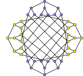
Figure 4: One of the two maximal cubic graphs with $n=40$, $D=6$. It has automorphism group of order 480.

The two graphs of order 42 have the same spectrum. They both exhibit a tripe-tree structure as shown in figure 5.

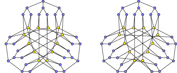
Figure 5: Two maximal cospectral graphs on 42 vertices with $D=6$. Each yellow vertex is adjacent to all three Bethe trees in blue. The graph on the left is symmetric under rotation by 120 degrees as well as reflection in vertical axis, and has automorphism group of order 48. The graph on the right is not, and has automorphism group of order 24. Both have girth 8. Their spectrum is $\pm 3,\pm\sqrt{5}^{(8)},\pm 2,\pm\sqrt{2}^{(4)},\pm 1^{(2)},0^{(10)}$.

3.5 Degree 3, Diameter 7

For diameter $7$ we found $45$ graphs that achieve the AC bound. All of these graphs are bipartite with girth $8$, and were constructed using a method that seems useful in this context. The procedure begins with two copies of the degree $3$ Moore tree of depth $3$, as shown Figure 6. To complete the graph we consider only edges that join leaf vertices in of the Moore trees to leaf vertices in the other tree. In the figure, these would be edges joining red vertices and green vertices. There are only $144$ such edges, so complete search for such graphs can be done quickly. Such a search results in the $45$ graphs mentioned earlier. Among them, the highest automorphism group has order 48, represented by a single graph.

Figure 6: Starting configuration for generating graphs with diameter $7$ and maximum AC.

3.6 Degree 3, Diameter 8

In this case, max AC=$3-\sqrt{6}\approx 0.5505.$ We found $18$ cubic graphs of order $68$ that attain this bound. All of these graph have girth $9$. None of the graph are particularly symmetric, with automorphism groups ranging in size from $1$ to $24$. The graphs were constructed by searching girth $9$ graphs of order $9$, and checking the diameter after a girth $9$ graph was constructed.

3.7 Degree 3, Diameter 9

For diameter $9$, by Theorem 1.3, all maximal graphs have exactly 92 vertices. We again used the double tree method outlined in §3.5. We generated a total of around 1500 maximal graphs which took several days of computing on 6 processors at once. Of these, 481 were distinct (non-isomorphic). All of them had girth 10. The following table lists the statistics for group size of this collection:

group size 48 32 24 16 12 8 4 2 1

#graphs 1 3 2 7 2 34 101 242 86

Note that this is not an exhautsive list, but we estimate that the actual number is close to 500. Note that the cubic cage of girth $10$ has order $70$ [29].

3.8 Degree 4, Diameter 3

The unique maximal maximal graph with $D=3$ is the modified bipartite graph described in §5.2. Figure 7 shows its symmetric realization.

Figure 7: A $4$-regular graph with diameter $3$ and AC = $3.0$.

3.9 Degree 4, Diameter 4

There are two maximal $4$-regular graphs of diameter $4$ on 16 vertices that achieve the AC bound of $2.0$: the $4$-cube and its cospectral mate [30], the Hoffman graph, shown in Figure 8. Note that $n=16$ is the smallest possible, see Theorem 1.5.

Figure 8: Two maximal graphs for $d=4,D=4,n=16.$ with AC=2. Left: the Hoffman graph. Right: the 4-Cube (Tesseract) graph

In §5.4 we exhibit a maximal graph with 30 vertices based on projective plane techniques (figure 9).

Figure 9: Maximal graph for $d=4,D=4,n=30$ with AC=2. There are 10 triplets of vertices, labelled A to J, that are at distance 4 from each other. Its automorphism group is of order 720.

Using tables of quartic regular graphs [25, 27] we found maximal graphs up to order 32. Overall, there are maximal graphs with 16, 22, 23, 24, 28, 30, and 32 vertices, see table in 3.12 for further information.

3.10 Degree 4, Diameter 5

Twelve graphs of degree $4$ and diameter $5$ were found. All have girth $6$ and all were found using the starting configuration of two Bethe trees as in figure 6.

3.11 Degree 6, Diameter 4

In §5.4 we construct a family of $D=4$ maximal graphs when $d$ is a power of prime, having $n=2d^{2}-2$ vertices. So $d=6$ is the smallest $d$ which is not part of that family. Nonetheless, we found a maximal graph using stochastic search algorithm.

3.12 Summary of diameter-maximal graphs

The table below summarizes our findings. For the column “#graphs”, a number in bold indicates that the corresponding class has been searched exhaustively, and no other graphs for the corresponding $n$ are expected. Otherwise, it is the number we managed to find, but there may be more. Note that we restricted the search to the girth as specified in the table. Where possible (for $n\leq 20$), we also confirmed using exhaustive search that no maximal graphs exist for girths smaller than indicated.

$d$	$D$	AC	$n$	#graphs	Comments
3	3	2	8	1	The $3$-cube, see §5.2.
3	4	1.2679	14 16 18	1 1 1	Graph 3H (see Figure 1(a)) Möbius Kantor Graph Pappus graph
3	5	1	20	5	All have girth $6$; includes the Desargues graph.
3	6	0.7639	32 34 36 38 40 42	2 2 2 1 2 2	Both have girth 7 Both have girth 7, cospectral Both have girth 8 Girth 8 Both have girth 8 Both have girth 8, cospectral
3	7	0.6571	$44$	45	All of have girth 8.
3	8	0.5505	68 80 90	12 1 3	Two of girth 8 and ten of girth 9 Girth 10 Girth 10
3	9	0.4965	92	$481$	All have girth 10
4	3	3	10	1	See §5.1.
4	4	2	16 17 19-21 22 23 24 28 30 32	6 0 0 3 2 2 1 1 1	Girth 4; group sizes: 6,8,12,32,48 (Hoffman), 384 (Tesseract) Girth 4: 193900 graphs, none maximal Girth 5 Girth 5, group sizes 2, 4, 8 Girth 5; group sizes 1, 4 Girth 5; co-spectral, group sizes 16, 16 Unique graph of girth 6 on 28 vertices Girth 6, see §5.4 and figure 9 Girth 6
6	4	3.5505	44	$\geq 1$	Not part of $D=4$ family of §5.4

4 Maximum AC for given girth and order

As mentioned in Theorem 1.4, girth-maximal graphs must necessarily be Moore graphs. This gives a severe restriction on existence of girth-maximal graphs. Conversely, all the Moore graphs we considered appear to be girth-maximal. This includes girth-6 projective plane family (see §5.3), Peterson graph on 10 vertices of girth 5, the cubic Tutte cage on 30 vertices of girth 8, and the cubic Benson cage of girth 12 on 126 vertices [29]. It remains an open question as to whether all known Moore graphs are girth-maximal.

We used the data from House of Graphs website [25] which contains complete enumeration of cubic graphs up to orders 64, particularly for higher girths. For each combination of order and girth, we computed the maximum AC. This is recorded in the tables below.

$g$	$n$	max AC	Comments
3	4 6 8 10 12 14 16 18	4 2 1.438447 1.120614 1 0.885092 0.82259 0.763932	Complete graph, maximal
4	6 8 10 12 14 16 18 20	3 2 1.438447 1.267949 1.068732 1 0.903097 0.845793	Modified bipartite, maximal, see §5.1
5	10 12 14 16 18 20 22	2 1.467911 1.289171 1.172909 1.043705 1 0.913969	Petersen graph, maximal

$g$	$n$	max AC	Comments
6	14 16 18 20 22 24	1.585786 1.267949 1.267949 1.064568 1 1	PG(2,2), maximal, see §5.3
7	24 26 28 30 32 30	1 0.94737 1 0.844084 0.864221 1
8	30 34 36 38 40 42	1 0.78568 0.763932 0.763932 0.763932 0.763932	Tutte graph, maximal
9	58 60 62 64	0.63766 0.697224 0.603671 0.633832	Next 3: 0.6031,0.6025,0.6011
12	126	0.5505	Benson graph, maximal

5 Maximal graph families

Here, we exhibit families of maximal graphs for infinitely many $d$: girth 3,4, and 6, and diameters 3 and 4.

5.1 Girth 3 and 4

The trivial cases are the girth-3 and girth-4 maximal graphs which are complete graph on $d+1$ vertices, and complete-bipartite graphs on $2d$ vertices. Their AC is well known to be $d+1$ and $d$ respectively, which are maximal.

5.2 Diameter 3

This is a modified bipartite graph on $2d+2$ vertices, illustrated here for the case of $d=4:$

It is constructed by starting with complete bipartite graph on $2d$ vertices, removing $d$ matching edges, and adding two extra vertices, each with $d$ edges connecting it to $d$ vertices of each of component. This graph has spectrum $\pm d$ (once)$,\ \pm 1$ ($d$ times each), so that $AC=d-1,$ which is maximal for $D=3.$

This maximal graph is in fact unique, which can be seen as follows. Maximal graph of odd diameter $D=2K-1$ must consist of two Bethe trees of $K$ levels whose leafs are connected to each-other. In the case of $D=3$, the two trees are simply two star graphs with $d$ leafs. Each leaf of the left star is connected to $d-1$ leafs of the right star and vice-versa. In other words, for each leaf on the left star, there is exactly one leaf on the right star to which it is not connected and vice-versa. Moreover, this is a one-to-one correspondence (otherwise there would be more than one leaf on the left star not connected to a single leaf on the right star). This shows that all maximal graphs with $D=3$ must be isomorphic.

5.3 Girth 6.

It is well known that a projective plane $PG(2,q)$, $q$ a prime power, is in fact a degree $d=q+1$ regular graph of girth 6, and is indeed one of the few Moore graphs [29]. Its spectrum is easy to compute, see for example [31, 32, 33]. From there it follows that $AC=d-\sqrt{d-1}$ which is maximal for girth 6. For completeness, we reproduce these arguments here.

Let us recall the construction of a projective plane graph. Given a degree $d,$ consider a finite field $F$ of size $q=d-1$ (such a field only exists when $q$ is a prime power). A line $L\in PG(2,q)$ is a non-zero tuple $\left(a,b,c\right)$ with $a,b,c\in F$, modded by an equivalence relation corresponding to scalar multiplication. More explicitly, a line can be represented uniquely by rescaling the first non-zero coordinate to one: either $\left(1,b,c\right)$ with $b,c\in F$ or $\left(0,1,c\right)$ with $c\in F$, or $\left(0,0,1\right).$ Correspondingly, there are $q^{2}+q+1$ such lines. A point $P=(x,y,z)$ in $PG(2,q)$ has the same form as a line. Then $PG(2,q)$ is a bipartite graph having $2(q^{2}+q+1)$ vertices. Half of the vertices are lines $L$, half are points $P$, and there is an edge between $L$ and $P$ if and only if $L\cdot P\equiv 0.$

One can easily check that $PG(2,q)$ is regular of degree $d=q+1;$ has $n=2d^{2}-2d+2$ vertices, has no four-cycles (and therefore has girth $g=6),$ and has diameter $D=3$. Let us compute its spectrum following [31, 32, 33].

The adjacency matrix has the form $A=\left[\begin{array}[c]{cc}0&B\\ B&0\end{array}\right]$ where $B_{ik}=\left\{\begin{array}[c]{c}1\text{, if }L_{i}\perp P_{k}\\ 0\text{, otherwise}\end{array}\right..$ Note that $B$ is symmetric since lines and points are identical and interchangeable in this geometry. Correspondingly, the eigenvalues of $A$ are given by $\lambda=\pm\sqrt{\mu}$, where $\mu$ is an eigenvalue of $M=B^{2}.$ Note that $M_{ij}=\sum_{k}B_{ik}B_{kj}$ so that $M_{ij}$ is number of points $P$ which are simultaneously orthogonal to both lines $L_{i}$ and $L_{j}$. It is easy to check that

$$M_{ij}=\left\{\begin{array}[c]{c}q+1,\text{ if }i=j\\ 1\text{ otherwise}\end{array}\right.$$

Correspondingly, the eigenvalues of $M$ are $\mu=q=d-1$ (with multiplicity $q^{2}+q$), and $q^{2}+2q+1=d^{2}$ with multiplicity one. So the spectrum of $A$ consists of four eigenvalues: $\pm d,$ and $\pm\sqrt{d-1}$ with multiplicity $d(d-1).$ It follows that $AC=d-\sqrt{d-1}.$

5.4 Diameter 4.

Here, we will construct a $d-$ regular graph $G$ which is a subgraph of $PG(2,d)$ (with $d$ a prime power). Its order is $2d^{2}-2.$ This graph is likely to be the same as girth-6 graph of same order from [34, 35, 36], although we use a different construction here to compute its spectrum and girth.

Consider the subset of lines and points of $PG(2,d)$ of the form $\left(1,b,c\right)$, where one of $b,c$ are non-zero. For example when $d=3,$ there are 8 such lines and points, namely:

$$\left(1,0,1\right),\ (1,0,2);\ \ \ (1,1,0),\ (1,2,0);\ \ \ (1,1,1),\ (1,2,2);\ \ \ (1,1,2),\ (1,2,1).$$ (28)

It is easy to see that such graph is regular of degree $d;$ has $n=2d^{2}-2$ vertices, its girth is $g=6$ and its diameter is $D=4.$ We start by showing the latter here.

Consider two distinct lines $L_{1}=\left(1,a_{1},b_{1}\right)$ and $L_{2}=\left(1,a_{2},b_{2}\right).$ They are adjacent to the same point $P=\left(1,x,y\right)$ if and only if $\left(\begin{array}[c]{cc}a_{1}&b_{1}\\ a_{2}&b_{2}\end{array}\right)\left(\begin{array}[c]{c}x\\ y\end{array}\right)=\left(\begin{array}[c]{c}-1\\ -1\end{array}\right).$ If this system has a solution, then the distance between these two lines is 2. In the opposite case, we have that $\left(a_{2},b_{2}\right)=c\left(a_{1},b_{1}\right)$ for some $c\in F.$ In this case, pick a point $P$ perpendicular to $L_{1}.$ This point has $d-1$ other lines that are perpendicular to it. Pick one such line, call it $L_{3}=\left(1,a_{3},b_{3}\right).$ Note that $\left(a_{3},b_{3}\right)\neq c\left(a_{2},b_{2}\right)$. for any $c\in F.$ But then $\operatorname{dist}(L_{2},L_{3})=2=\operatorname{dist}(L_{3},L_{1})$ so that $\operatorname{dist}(L_{1},L_{2})=4.$ Similar argument shows that $\operatorname{dist}(L,P)\leq 3$ for any line $L$ and point $P.$

Next we compute the spectrum of $G.$ As before, its spectrum is given by $\lambda=\pm\sqrt{\mu}$, where $\mu$ is an eigenvalue of matrix $M=B^{2};$ where $B_{ij}=\left\{\begin{array}[c]{c}1\text{, if }L_{i}\perp P_{k}\\ 0\text{, otherwise}\end{array},\right.$ with $M_{ij}$ being the number of points $P$ which are orthogonal to both lines $L_{i}$ and $L_{j}$. For example, in the case of $d=3$ and with lines $L_{1}\ldots L_{8}$ and points $P_{1}\ldots P_{8}$ ordered as in (28), the corresponding matrices are

$$B=\left[\begin{array}[c]{cccccccc}0&1&0&0&0&1&1&0\\ 1&0&0&0&1&0&0&1\\ 0&0&0&1&0&1&0&1\\ 0&0&1&0&1&0&1&0\\ 0&1&0&1&1&0&0&0\\ 1&0&1&0&0&1&0&0\\ 1&0&0&1&0&0&1&0\\ 0&1&1&0&0&0&0&1\end{array}\right];\ \ \ M=\left[\begin{array}[c]{cccccccc}3&0&1&1&1&1&1&1\\ 0&3&1&1&1&1&1&1\\ 1&1&3&0&1&1&1&1\\ 1&1&0&3&1&1&1&1\\ 1&1&1&1&3&0&1&1\\ 1&1&1&1&0&3&1&1\\ 1&1&1&1&1&1&3&0\\ 1&1&1&1&1&1&0&3\end{array}\right].$$

Zeros in $M$ correspond to lines that are at distance 4 from each other and ones to lines at distance 2 from each other. To see this more generally, group $d^{2}-1$ lines into distinct classes $C_{1},\ldots,C_{d+1}$ of $d-1$ members each, such that lines $L_{i}=\left(1,a_{1},b_{1}\right)$ and $L_{j}=\left(1,a_{2},b_{2}\right)$ are in the same class if and only if $\left(a_{2},b_{2}\right)=c\left(a_{1},b_{1}\right)$ for some $c\in F\backslash\left\{0\right\}.$ Then $M_{ij}=0$ iff $i\neq j$ and $i,j\in C_{k}$ for some $k;$ otherwise $M_{ij}=1$ if $i\neq j$ and $M_{ij}=d$ if $i=j.$

Define an eigenvector $v$ such that $\sum_{j\in C_{k}}v_{j}=0$ for each class $C_{k},k=1\ldots d+1.$ This gives $d+1$ linear equations, so there is a total of $\left(d^{2}-1\right)-(d+1)=d^{2}-d-2$ independent such eigenvectors; and moreover it is easy to check that $Mv=dv.$ Thus, $M$ has an eigenvalue $\mu=d$ of multiplicity $d^{2}-d-2.$ Next, for each $k=1\ldots d+1$, define $v$ such that $v_{j}=V_{k}$ if $j\in C_{k};$ and moreover choose $V_{k}$ such that $\sum_{1}^{d+1}V_{k}=0.$ Note that there are $d$ independent such choices. Then $Mv=(d-(d-1))v=v.$ This gives an eigenvalue of $\mu=1$ of multiplicity $d.$ Finally, the eigenvector $v=(1\ldots 1)$ yields an eigenvalue of $d^{2}.$

In conclusion, the spectrum of $G$ is $\pm d$ (once)$,\pm\sqrt{d}$ ($d^{2}-d-2$ times), and $\pm 1$ ($d$ times). Subsequently, $AC=d-\sqrt{d}.$

Summary. The following table summarizes some facts about attainable bounds with respect to girth and diameter. Bold font indicates whether it is maximal with respect to girth or diameter.

$d$	$D$	$g$	$n$	AC	Comments
any $d$	1	3	$d+1$	$d+1$	complete graph on $d$ vertices
any $d$	2	4	$2d$	$d$	complete-bipartite graph
any $d$	3	4	$2d+2$	$d-1$	Modified bipartite graph
$p^{\alpha}+1$, $p$ prime	3	6	$2d^{2}-2d+2$	$d-\sqrt{d-1}$	Projective plane $PG\left(2,d-1\right)$
$p^{\alpha}$, $p$ prime	4	6	$2d^{2}-2$	$d-\sqrt{d}$	Subset $PG\left(2,d\right)^{-}\subset PG\left(2,d\right)$

6 Discussion and open questions

We exhibited tight upper bounds for AC for regular graphs with respect to girth or diameter. While the girth bound is attainable only by Moore graphs – which imposes a severe restriction on $g$ – the diameter bound is less restricting but is nonetheless is very rarely attained. Using a combination of stochastic algorithms and exhaustive search, we produced examples of maximal graphs for $d=3$ and $D\leq 9,$ as well as $d=4$ and $D\leq 6.$ There are many interesting open questions – both computational and theoretical – that we hope the reader will be tempted to explore.

Complete lists of cubic and quartic graphs for small orders suggests that for a fixed $n$, the graph with a maximum AC also have the maximum possible girth; see table in §4. This was the key insight that allowed us to find diameter-maximal graphs: we simply searched for graphs of highest possible girth for a given order, and generated as many such graphs as we could; then hope that a small subset of these would end up being diameter-maximal. This leads to our first conjecture.

Conjecture 6.1

For a fixed degree $d$ and order $n$, the graph with maximum possible AC has the maximum possible girth.

In fact, the table in §4 suggests an even stronger conjecture:

Conjecture 6.2

Let $f(g;d,n)$ be the maximum possible AC among the graphs of given degree $d,$ order $n$ and girth $g.$ Then $f(g;d,n)$ is an increasing function of $g.$

Our search for diameter-maximal also suggests the following conjecture:

Conjecture 6.3

    

• A diameter-maximal graph of odd diameter $D$ must have girth $g=D+1$.

• A diameter-maximal graph of even diameter $D$ must have girth of either $g=D,D+1$ or $D+2.$

The complexity of finding maximal graphs increases tremendously with larger $D.$ We spent significant time searching for $D=10$ maximal cubic graphs, but did not find any as of this writing. We state this as an open problem.

Open question 6.4

Find a $D=10$ maximal cubic graph, or show it doesn’t exist.

We showed that girth-maximal graphs are necessarily Moore graphs, which imposes a severe restriction on $g$. The only possible Moore graphs are $d=3$, $7$, and possibly $57$, and $g=5$, or else $d-1$ is a prime power and $g=6$, $8$ or $12$. [29]). We also showed that Moore graphs with $g=6$ are maximal for any $d$ which is a prime power plus one. In addition, we verified that Moore graphs with $d=3$ and $g=5,8\,$and $12$ are also maximal. What aboutother $d?$

Open question 6.5

Are all Moore graphs girth-maximal?

In contrast to girth-maximal, we found that diameter-maximal graphs exist for all $D<10$ when $d=3$. Do they exist for all $D?$

Open question 6.6

Do diameter-maximal graphs exist for any $D?$

We described a family of diameter-maximal graphs for $D=4$ when $d$ is a prime power. A computer search also revealed a maximal graph with $d=6,D=4.$ The smallest unsettled case with $D=4$ is therefore $d=10.$

Open question 6.7

Find maximal graphs with $D=4$ when $d$ is not a prime power. Find a general family of maximal graphs for $D=5$ and higher.

Finally, a big difference between odd and even diameters is that maximal graphs for odd diameter exist only for a specific value of $n$ given in Theorem 1.3, whereas even-diameter graphs exist for a range of values of $n$. Theorem 1.5 gives the lower bound for such $n,$ although it is not always attained. What about the upper bound?

Open question 6.8

For even $D$, what is the largest $n$ that admits a maximal graph?

For example, Theorem 1.3 gives a lower bound of $n=28$ when $d=3,\ D=8;$ we found examples of maximal graphs with $n=68,80,$ and $90$. Maximal graphs for $D=9$ require $n=92.$ Do does there exist a maximal graphs with $D=8$ and $n=92?$ Do maximal graphs exist for values of $n<68?$ For other values of $n?$

We mostly concentrated on diameter-maximal graphs. While girth-maximal graphs do not generally exist due to the Moore graph constraint, there is some graph that maximizes AC. Section 4 lists some of these records based on complete enumeration of cubic graphs of high girths [25, 26]. What about higher $n$ or $g$, where complete enumeration is impossible?

Open question 6.9

For a given girth or given graph order $n$, find an efficient algorithm to produce $d-$regular graph with as high AC as possible.

A well-known Ghosh-Boyd algorithm [5] generating well-connected graphs – when modified to produce regular graphs only – does much worse than the optimal. For example, running modified Ghosh-Boyd algorithm 100 times with $d=3,n=64$ yields an average AC of $0.45$ (std=0.018, max=0.489 over 100 simulations). Moreover almost all runs produce girth 5 or 6; none produced more than 7. By contrast, the record graph (see §4) is a graph of girth 9 and AC=0.6338; the average AC of all 1408813 girth-9 such graphs is $0.53$ (std=0.018), quite far from the Ghosh-Boyd result. We also generated random cubic graphs on 64 vertices. These have average AC of 0.25 (std=0.047, max=0.367 over 100 simulations). Finding the record graph is an extremely time-consuming task; it takes thousands of computer hours to find the record AC using the full enumeration compared to a fraction of a second to run the Ghosh-Boyd algorithm. Finding an efficient algorithm that does significantly better than Ghosh-Boyd is an important problem.

Appendix A Code for maximal graph generation

Many of the graph discussed in the paper were found by a search procedure outlined below. The C code is available for download [28], along with a collection of maximal graphs.

The procedures uses a $Graph$ data structure that contains

• The adjacency list,

• The adjacency matrix,

• The edge list,

• The edge count, denoted $edgecount$,

• The target, i.e., the number of edges in a completed graph.

The procedure begins by initializing the graph. This initialization either results in a graph with no edges or else a forest. Examples of forests that might be used include a Moore tree or pair of trees like the ones shown in Figure 6.

The main loop of the procedure begins by calling the Makelist procedure which creates a list of edges that could be added to the graph without violating the degree and girth constraints. If the initial graph has no edges, then for the first iteration this list will contain all possible edges. The list is then sorted by the sum of the degrees of the two vertices in the edge, in decreasing order. Candidate edges with the same degree sum are sorted randomly. This sorting by decreasing degree sum is the single most important idea in the procedure. Without it, the procedure will be successful only on very small graphs. With it, new results can be obtained. For example, the $(4,7)$-cage was found using this method [37].

At the end of the for-loop in the procedure, we have either completed the graph, in which case we are done, or we remove a small number of edges and try again. The number of edges removed is typically very small (usually $1$), but if no increase in the maximum number of edges attained is realized for a large number of iteration through the while loop, the number of edges removed can be slowly increased, until reaching some maximum value, after which it is reset to the small value.

Algorithm 1 Graph Search

procedure Search($graph$,$initialState$)

    Initialize Graph

    while $edgecount<target$ do $\triangleright$ The $target$ is $degree*order/2$

         $feasible\leftarrow Makelist(graph)$

         $SortEdges(feasible,graph)$

         for each edge $e$ in $feasible$ do

             SortEdges($graph$)

             if EdgeCheck($e$,$graph$) then

                 AddEdge($e$, $graph$)

             end if

             Remove $e$ from $feasible$

         end for

         if $edgecount==target$ then

             Return

         end if

         Remove a few random edges

    end while

end procedure

References

- [1] Fiedler, M. (1973) Algebraic connectivity of graphs. Czechoslovak Mathematical Journal 23, 298–305.
- [2] de Abreu, N. M. M. (2007) Old and new results on algebraic connectivity of graphs. Linear algebra and its applications 423, 53–73.
- [3] Olfati-Saber, R & Murray, R. M. (2004) Consensus problems in networks of agents with switching topology and time-delays. Automatic Control, IEEE Transactions on 49, 1520–1533.
- [4] Olfati-Saber, R. (2005) Ultrafast consensus in small-world networks. American Control Conference, 2005. Proceedings of the 2005 pp. 2371–2378.
- [5] Ghosh, A & Boyd, S. (2006) Growing well-connected graphs. 2006 45th IEEE Conference on Decision and Control pp. 6605–6611.
- [6] Hoory, S, Linial, N, & Wigderson, A. (2006) Expander graphs and their applications. Bulletin of the American Mathematical Society 43, 439–561.
- [7] Lubotzky, A. (2012) Expander graphs in pure and applied mathematics. Bulletin of the American Mathematical Society 49, 113–162.
- [8] Friedman, J. (1993) Some geometric aspects of graphs and their eigenfunctions. Duke Math. J. pp. 487–525.
- [9] Alon, N. (1986) Eigenvalues and expanders. Combinatorica 6, 83–96.
- [10] Nilli, A. (2004) Tight estimates for eigenvalues of regular graphs. Electron. J. Combin 11, 1–4.
- [11] Ogiwara, K, Fukami, T, & Takahashi, N. (2015) Maximizing algebraic connectivity in the space of graphs with a fixed number of vertices and edges. IEEE Transactions on Control of Network Systems 4, 359–368.
- [12] Shahbaz, K, Belur, M. N, & Ganesh, A. (2023) Algebraic connectivity: local and global maximizer graphs. IEEE Transactions on Network Science and Engineering.
- [13] Mosk-Aoyama, D. (2008) Maximum algebraic connectivity augmentation is NP-hard. Operations Research Letters 36, 677–679.
- [14] Kolokolnikov, T. (2015) Maximizing algebraic connectivity for certain families of graphs. Linear Algebra and its Applications 471, 122–140.
- [15] Wang, H & Van Mieghem, P. (2008) Algebraic connectivity optimization via link addition. Proceedings of the 3rd International Conference on Bio-Inspired Models of Network, Information and Computing Sytems p. 22.
- [16] Kim, Y. (2009) Bisection algorithm of increasing algebraic connectivity by adding an edge. IEEE Transactions on Automatic Control 55, 170–174.
- [17] Li, G, Hao, Z. F, Huang, H, & Wei, H. (2018) Maximizing algebraic connectivity via minimum degree and maximum distance. IEEE Access 6, 41249–41255.
- [18] Kolokolnikov, T. (2021) It is better to be semi-regular when you have a low degree. arXiv preprint arXiv:2112.14289.
- [19] Cioaba, S. M, Koolen, J. H, Nozaki, H, & Vermette, J. R. (2016) Maximizing the order of a regular graph of given valency and second eigenvalue. SIAM Journal on Discrete Mathematics 30, 1509–1525.
- [20] Cioabă, S. M. (2020) Eigenvalues of graphs and spectral moore theorems. arXiv preprint arXiv:2004.09221.
- [21] Pegg Jr, E & Exoo, G. (2009) Crossing number graphs. The Mathematica Journal 11, 161–170.
- [22] Bussemaker, F & Cvetković, D. (1976) There are exactly 13 connected, cubic, integral graphs. Publikacije Elektrotehničkog fakulteta. Serija Matematika i fizika pp. 43–48.
- [23] Salamon, T. (2022) On the algebraic connectivity of graphs. (Dalhousie University, MSc thesis).
- [24] Friedman, J. (1991) On the second eigenvalue and random walks in random d-regular graphs. Combinatorica 11, 331–362.
- [25] Coolsaet, K, D’hondt, S, & Goedgebeur, J. (2023) House of graphs 2.0: A database of interesting graphs and more. Discrete Applied Mathematics 325, 97–107. Available at https://houseofgraphs.org.
- [26] McKay, B, Myrvold, W, & Nadon, J. (1998) Fast backtracking principles applied to find new cages. Proceedings of the ninth annual ACM-SIAM symposium on Discrete algorithms pp. 188–191.
- [27] Meringer, M. (1999) Fast generation of regular graphs and construction of cages. Journal of Graph Theory 30, 137–146.
- [28] (2023) A database of maximal graphs from this paper and code is available from the authors (http://www.mathstat.dal.ca/~tkolokol/maxgraphs).
- [29] Exoo, G & Jajcay, R. (2013) Dynamic Cage Survey. Electronic Journal of Combinatorics DS16, 1–55.
- [30] Hoffman, A. J. (1963) On the polynomial of a graph. American Math Monthly 70, 30–36.
- [31] Ryser, H. J. (1955) Geometries and incidence matrices. The American Mathematical Monthly 62, 25–31.
- [32] Hoffman, A. (1965) On the line graph of a projective plane. Proceedings of the American Mathematical Society 16, 297–302.
- [33] Godsil, C, Holton, D. A, & McKay, B. (1977) The spectrum of a graph. Lecture Notes in Math 622, 91.
- [34] Abreu, M, Funk, M, Labbate, D, & Napolitano, V. (2006) On (minimal) regular graphs of girth 6. Australasian Journal of Combinatorics 35, 119.
- [35] Araujo-Pardo, G, Balbuena, C, & Héger, T. (2010) Finding small regular graphs of girths 6, 8 and 12 as subgraphs of cages. Discrete mathematics 310, 1301–1306.
- [36] Araujo-Pardo, G & Balbuena, C. (2011) Constructions of small regular bipartite graphs of girth 6. Networks 57, 121–127.
- [37] Exoo, G, McKay, B. D, Myrvold, W, & Nadon, J. (2011) Computational determination of (3, 11) and (4, 7) cages. Journal of Discrete Algorithms 9, 166–169.