Polynomially knotted $2$ Spheres

Abstract.

We show that every proper, smooth 2-knot is ambient isotopic to a polynomial embedding from $\mathbb{R}^{2}$ to $\mathbb{R}^{4}$. This representation is unique up to a polynomial isotopy. Using polynomial representation of classical long knots we show that all twist spun knots posses polynomial parametrization. We construct such parametrizations for few spun and twist spun knots and provide their $3$ dimensional projections using Mathematica.

Tumpa Mahato

Rama Mishra

1. Introduction

Higher dimensional knot theory has attracted a lot of interest by knot theorists recently. By an n knot one means a smooth, proper, locally flat embedding of $S^{n}$ in $S^{n+2}$. Moving from classical knots, the simplest situation is to understand knotting of $S^{2}$ in $S^{4}$ or in $\mathbb{R}^{4}$. In fact, studies are being done on any surface getting knotted inside four dimensional space and 2-knots are just a special case. Notion of ambient isotopy can be defined as in the case of classical knots. The central problem will remain the same: classify all 2-knots on the basis of ambient isotopy.

Similar to the classical knots, a diagrammatic theory ([4]) and a braid theory ([12]) has been developed. Both theories have provided many interesting invariants for 2-knots. In case of classical knots we have encountered many numerical invariants, whose computations become easy using a suitable parametrization. Some interesting parametrizations are Fourier knots and Polynomial knots. While Fourier knots represent compact images, polynomial knots can provide only long knots. Polynomial knots are important because they bring an algebraic flavour into knot theory. One point compactification of a polynomial knot is a classical knot and projective closure of a polynomial knot is a knot in $\mathbb{R}P^{3}.$ Polynomial knots are extensively studied by Shastri [10], Mishra-Prabhakar [8], Durfee-Oshea [5]. Explicit polynomial representation for all knots up to $8$ crossings can be found in [8].

In this paper, we would like to discuss about parametrizing $2$-knots using polynomial functions. Since a $2$-knot is a proper, smooth, locally flat embedding of $S^{2}$ in $S^{4}$, removing a point from $S^{2}$ and the corresponding image under the embedding in $S^{4}$ we get an embedding of $\mathbb{R}^{2}$ to $\mathbb{R}^{4}$. We will call this embedding a long $2$-knot. We provide an explicit proof for the fact that every long $2$-knot is ambient isotopic to a polynomial embedding of $\mathbb{R}^{2}$ in $\mathbb{R}^{4}$. We also show that any two polynomial embeddings of $\mathbb{R}^{2}$ in $\mathbb{R}^{4}$ which are ambient isotopic are in fact polynomially isotopic. The idea of the proof is similar to the classical case [11].

We also address the problem of explicitly constructing a polynomial parametrization for a given $2$-knot. We begin with taking the simplest $2$-knots which are obtained from classical knots, such as Spun Knots, first introduced by Emil Artin [2]. Then we move to twist spun knots [16]. Obtaining a polynomial parametrization for these classes of knots is relatively simple because we can use the existing polynomial representation of classical knots [8] which can be brought into the form suitable for spin construction or twist spin construction. In this paper we explicitly provide the steps to parametrize spun knots and twist spun knots using polynomial functions and present their $3$ dimensional projections using Mathematica.

This paper is organized as follows: Section 2 is divided into two subsections. Section 2.1 includes the basic definitions required to study the $2$-knots. In Section 2.1 we provide a brief exposition to polynomial parametrization of classical knots. We show that for every classical long knot there exists a polynomial embedding $\phi:\mathbb{R}\to\mathbb{R}^{3}$ defined by $\phi(t)=(x(t),y(t),z(t))$ such that for some closed interval $[a,b]$ image of $\phi$ outside $[a,b]$ contains no knotting, $z(a)=z(b)=0$ and $z(t)>0$ for $t\in(a,b)$. We use this embedding to construct spun knots. In Section 3, we provide a detailed proof that for all long $2$-knots, polynomial representation exists and is unique up to a polynomial isotopy. In Sections 4.1 and 4.2 we provide detailed algorithm to write polynomial representation of spun knots and twist spun knots respectively. We write down explicit parametrization for spun trefoil and spun figure eight knot and also $k$ twist spun trefoil for $k=1,2,3$ and $10$.

2. Prerequisites

2.1. $2$-knots

Definition 2.1.

An embedding of a manifold $K$ in a manifold $M$ is called proper if $\partial K=K\cap\partial M$.

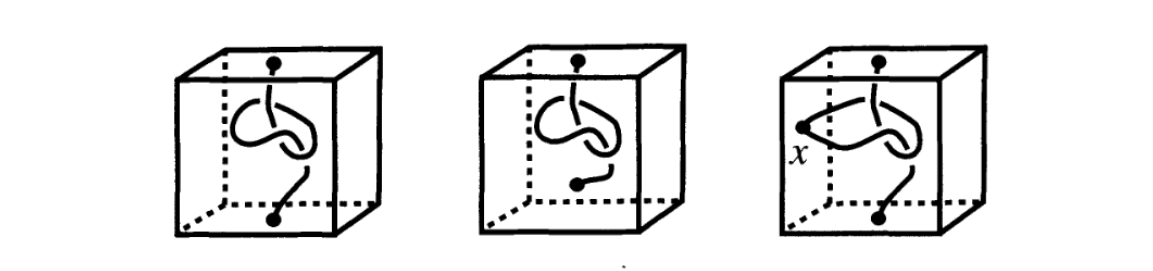
Figure 1. proper and non-proper embedding. Only the left most figure is a proper embedding.

Definition 2.2.

Let $K$ be a properly embedded k-manifold in an m-manifold $M$. Then $K$ is said to be locally flat at a point $x\in K$ if there exists a regular neighbourhood $N$ of $x$ in $M$ such that the pair $(N,N\cap K)$ is homeomorphic to a standard ball pair $(D^{m},D^{k})$. We say that $K$ is locally flat if it is locally flat at every point of $M.$

Non-locally flat embeddings exist. An example can be seen in [12].

Definition 2.3.

A locally flat embedding of $S^{2}$ in $\mathbb{R}^{4}$ or $S^{4}$ is called a $2$-knot.

Definition 2.4.

A proper, locally flat embedding of $R^{2}$ in $R^{4}$ is referred as a long $2$-knot.

Note that every $2$-knot will give rise to long $2$-knot by removing one point from $S^{2}$ and the image of that point from $S^{4}$ and consider the restriction of the embedding.

Definition 2.5.

Two $2$-knots $K_{1}$ and $K_{2}$ are said to be equivalent if there exists an orientation preserving diffeomorphism $h:S^{4}\to S^{4}$ such that $h(K_{1})=K_{2}$.

To study $2$-knots, we will need to project them on suitable $3$-dimensional space. To be able to understand the projection we restrict ourselves to long $2$-knots, i.e., proper, locally flat embeddings of $\mathbb{R}^{2}$ in $\mathbb{R}^{4}$. Thus projections will amount to understanding the image of maps from $\mathbb{R}^{2}\to\mathbb{R}^{3}$.

Definition 2.6.

Let $\phi:S^{2}\to\mathbb{R}^{4}$ be a $2$-knot. A projection $\pi:\mathbb{R}^{4}\to\mathbb{R}^{3}$ is said to be a regular projection if the composition $\pi\circ\phi:S^{2}\to\mathbb{R}^{3}$ is a smooth immersion.

Remark 2.1.

In general there may not exist a regular projection for a given $2$-knot. However, it has been proved [6] that for every $2$-knot $K$ in $\mathbb{R}^{4}$ there exists a $2$-knot $\tilde{K}$ which is ambient isotopic to $K$ and for $\tilde{K}$ a regular projection exists.

Remark 2.2.

In a regular projection, the image of $S^{2}$ in $\mathbb{R}^{3}$ is an immersion, hence the derivative map is injective at each point of $S^{2}$. Thus the singular set (points where the map fails to be one one) will consist of finite number of double point sets and triple points.

Remark 2.3.

A $2$-knot diagram consists of the projected image by a regular projection and a display of over/under information on each double point set and on each triple point.

Figure 2 gives an idea of how a $2$-knot diagram looks like.

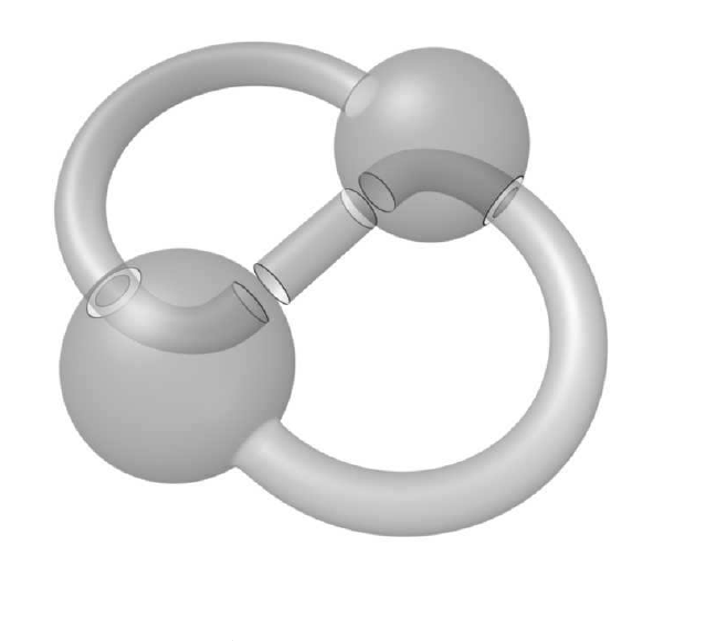
Figure 2. Broken surface diagram of a 2-knot

Artin [2] introduced a way to construct $2$-knots by spinning a knotted arc in $\mathbb{R}^{3}$ around $\mathbb{R}^{2}$. These types of knots are called Spun Knots. Spun knots are the simplest class of $2$-knots. Their construction is described as follows: In $\mathbb{R}^{4}$, consider the upper half space

$$\mathbb{R}^{3}_{+}=\Big{\{}(x_{1},x_{2},x_{3},0):x_{3}\geq 0\Big{\}}$$

with the boundary

$$\partial\mathbb{R}^{3}_{+}=\mathbb{R}^{2}=\Big{\{}(x_{1},x_{2},0,0)\Big{\}}$$

We can spin any point $x=(x_{1},x_{2},x_{3},0)$ in $\mathbb{R}^{3}_{+}$ about $\mathbb{R}^{2}$ by the following formula:

$$x_{\theta}=(x_{1},x_{2},x_{3}\,Cos\theta,x_{3}\,Sin\theta)$$

Now, to get a spin knot we choose an properly embedded arc $K$ i.e $K$ is embedded in $\mathbb{R}^{3}_{+}$ locally flatly and intersects $\partial\mathbb{R}^{3}_{+}$ transversely only at the endpoints. Then we spin $\mathbb{R}^{3}_{+}$ along $\mathbb{R}^{2}$ by $360^{o}$ and the locus of the arc gives a $2$-knot given by,

$$\Big{\{}(x_{\theta}:x\in K,0\leq\theta\leq 2\pi)\Big{\}}.$$

E.C. Zeeman in 1965 [16] generalized Artin’s spinning construction to twist spinning . In this case we imagine the knotted part of $K$ inside a 3-ball and rotate it on its axis while spinning the knot $K$ about the $xy$ plane. We can rotate the $3$-ball as many times as we want on its axis in $\mathbb{R}^{3}$. If we rotate it $k$ times then we will get a $k$-twist spun knot.

It is hard to visualize a two dimensional knot in four dimensional space. So, we see its projection on some $\mathbb{R}^{3}$. A projection of spun trefoil knot in $xzw$-upper half space is shown in Figure 8.

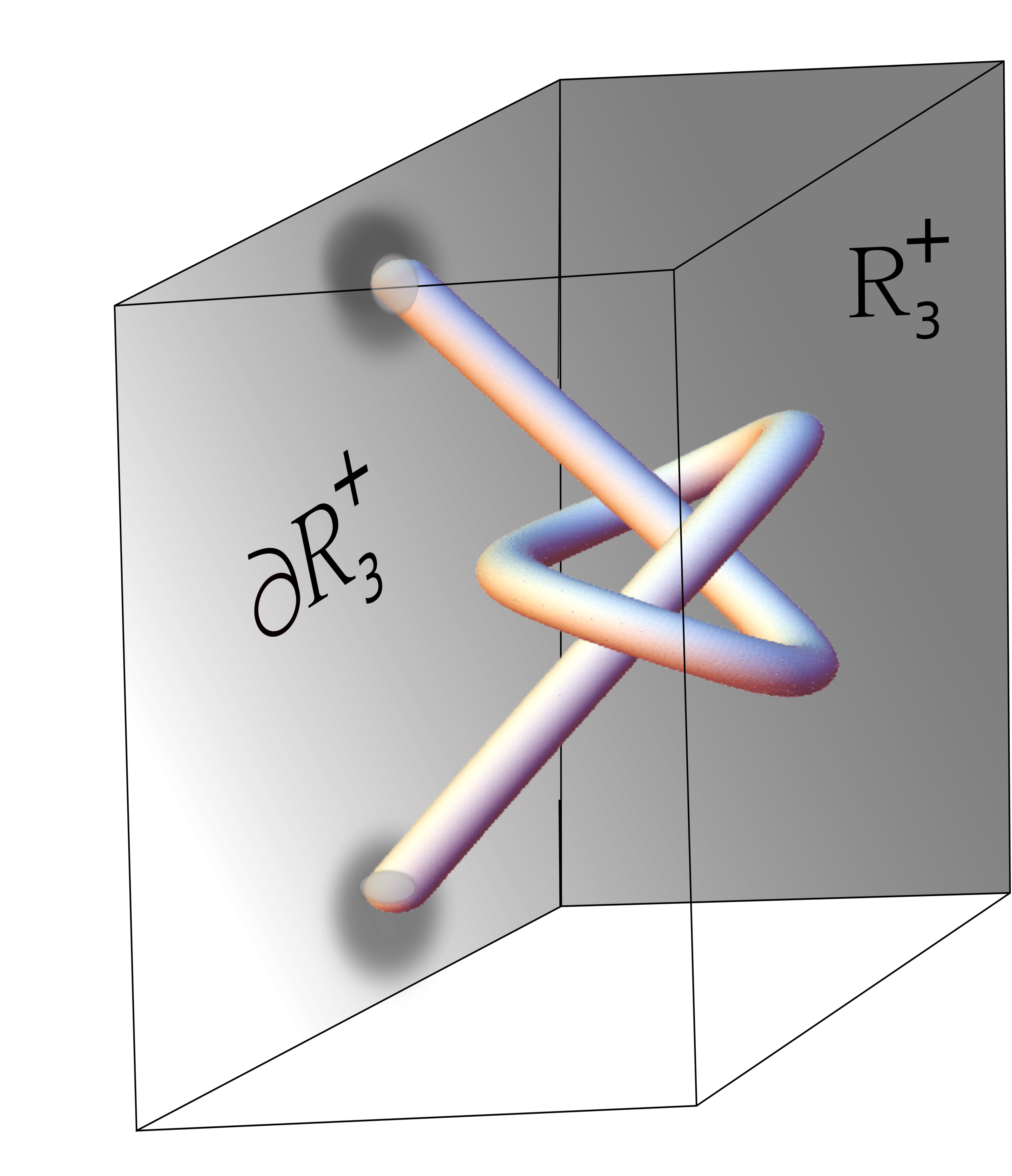
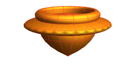
Figure 3. (a)Knotted arc in $\mathbb{R}^{3}_{+}$ with endpoints on $\partial\mathbb{R}^{3}_{+}$ ,(b)Projection of Spun Trefoil in $\mathbb{R}^{3}$

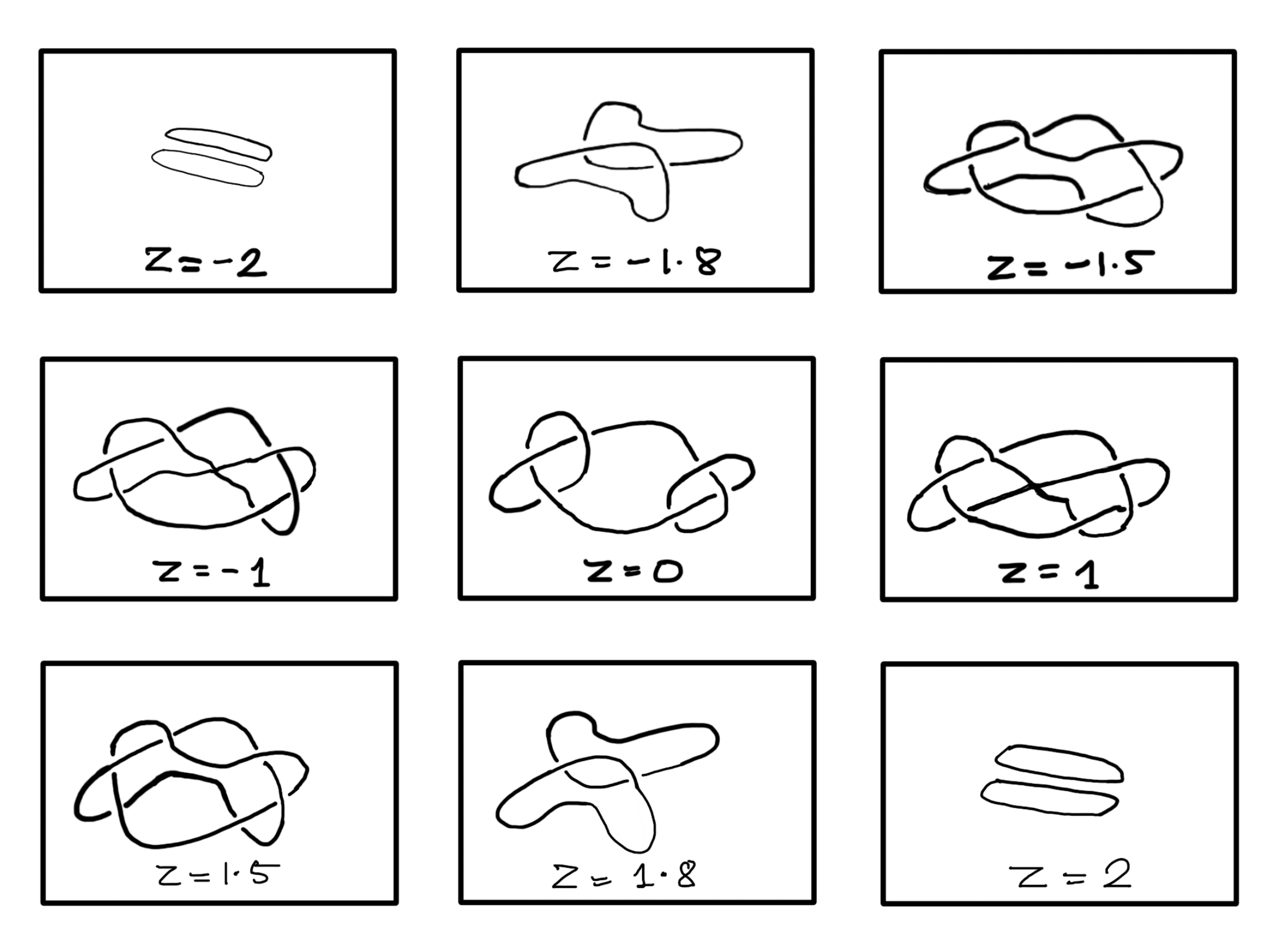
Figure 4. Motion picture of spun trefoil

Another way to visualize $2$-knots in $4$-space is to consider its intersection by hyper planes. Then each cross section will be a $1$-dimensional manifold which will be a knotted or unknotted $S^{1}$ at each cross section. A collection of such intersections is referred as a motion picture for the given $2$-knot. A motion picture of the spun trefoil is shown in Figure 4.

A detailed exposition on $2$ knots be found in [4] and [12].

2.2. Classical polynomial knots

It is easy to see that the ambient isotopy classes of classical knots ($S^{1}\subset S^{3}$) is in bijection with the ambient isotopy classes of long knots, i.e., the smooth embeddings of $\mathbb{R}$ in $\mathbb{R}^{3}$ which are proper and have asymptotic behaviour outside a closed interval. In 1994, the following theorems were proved:

Theorem 2.1 ([10], [11]).

For every long knot $K$ there exists a polynomial embedding $t\to(f(t),g(t),h(t))$ from $\mathbb{R}$ to $\mathbb{R}^{3}$ which is isotopic to $K$.

Theorem 2.2 ([11]).

If two polynomial embeddings $\phi_{0}:\mathbb{R}\to\mathbb{R}^{3}$ and $\phi_{1}:\mathbb{R}\to\mathbb{R}^{3}$ represent isotopic knots then there exists a one parameter family of polynomial embeddings $\phi_{t}:\mathbb{R}\to\mathbb{R}^{3}$ for each $t\in[0,1]$. We say that $\phi_{0}$ and $\phi_{1}$ are polynomially isotopic.

Both these theorems were proved using Weierstrass’ Approximation [15]. Later concrete polynomial embeddings representing few classes of knots were constructed and their degrees were estimated (eg., [8], [9]).

In all the constructions, the main idea is to fix a suitable knot diagram in mind and find real polynomials $f(t)$ and $g(t)$ such that the plane curve $(x(t),Y(t))=(f(t),g(t))$ provides the projection of the diagram. For this curve one can explicitly find the parameter pairs $(s_{i},t_{i})$ for which $f(s_{i})=f(t_{i})$ and $g(s_{i})=g(t_{i})$ for each $i$. Then depending upon the over/under crossing information we can construct a polynomial $h(t)$ which provides $h(s_{i})<h(t_{i})$ at an under crossing and $h(s_{i})>h(t_{i})$ at an over crossing. Note that in our construction we always project the knot on $XY$ plane and $Z$ coordinate provides the height function. All the crossings of the knot lie in the image of a closed interval $[a,b]$. We prove the following lemma which will be useful in Section 4.

Lemma 2.3.

Given a long knot $K$ there exists a polynomial embedding $t\to(x(t),y(t),z(t))$ from $\mathbb{R}\to\mathbb{R}^{3}$ such that for some interval $[a,b]$ $z(a)=z(b)=0$, $z(t)>0$ for $t\in(a,b)$ and there is no crossing outside $[a,b]$, for example the image looks as in Figure 5.

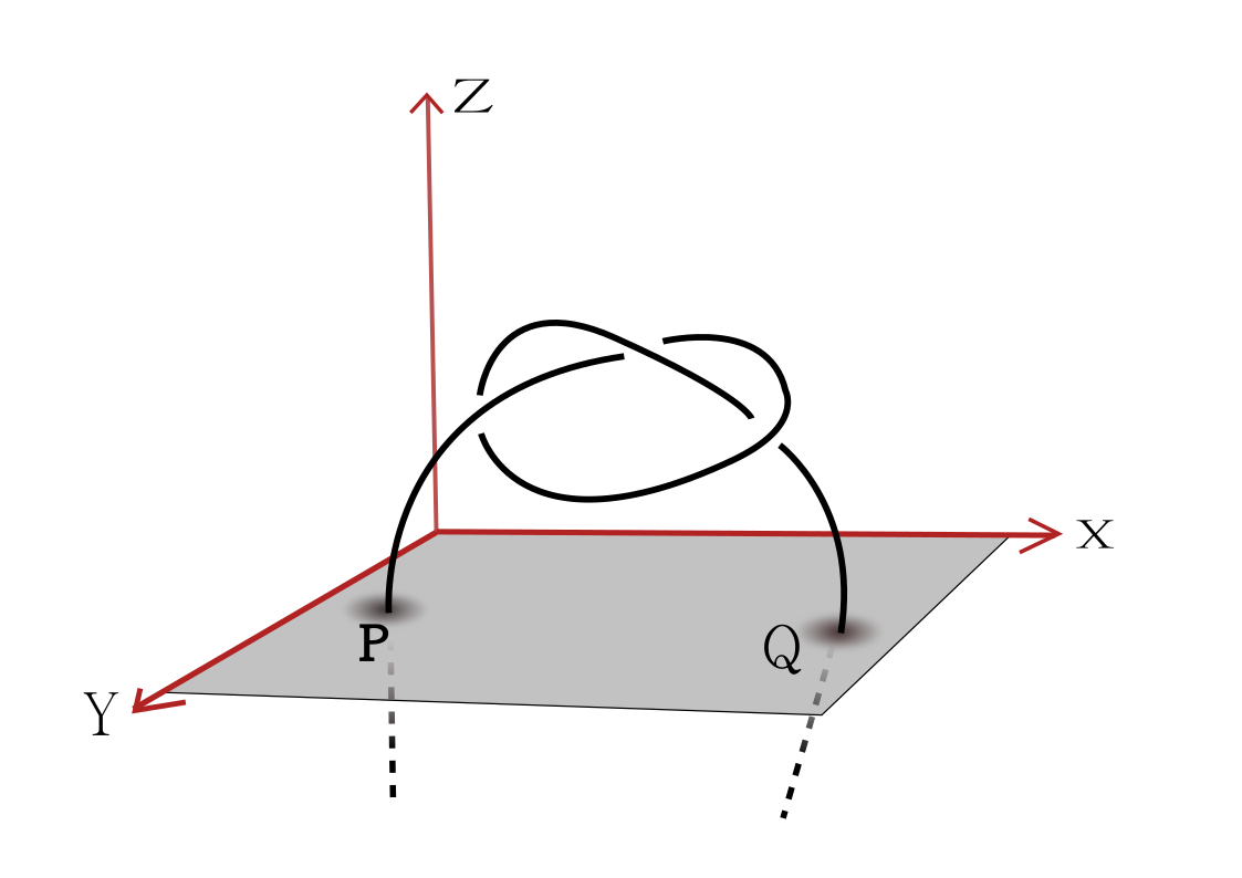
Figure 5. A long trefoil knot

Proof. We construct polynomials $f(t)$ and $g(t)$ such that the curve defined by $(x,y)=(f(t),g(t))$ represents a projection of $K$ on $XY$ plane. We choose the polynomial $h_{0}(t)$ which provides the over/under crossing information. Note that we can choose $h_{0}(t)$ to be an even degree polynomial. Now by adding a sufficiently large real number $R$ we can show that $h(t)=h_{0}(t)+R$ has exactly two real roots $a$ and $b$, $h(t)>0$ for $t\in(a,b)$ and all the double points of the projection lie inside $[a,b]$. This completes the proof.

Example 2.1.

As a demonstration, here is the embedding $t\to(t^{3}-3t,t^{4}-4t^{2},-t^{6}+2t^{5}+4.24t^{4}-8.48t^{3}-3.24t^{2}+6.48t+12)$ whose Mathematica plot is shown in Figure 6.

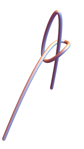
Figure 6. Mathematica plot of a polynomial embedding

3. Polynomial Representation of long $2$-knots

In this section we generalize the results in [11] in the context of $2$-knots.

Theorem 3.1.

Every smooth long $2$-knot $(\mathbb{R}^{2}\rightarrow\mathbb{R}^{4})$ has a polynomial representation.

Proof: Let $F$ be long 2-knot in $\mathbb{R}^{4}$ given by a smooth embedding $\phi:\mathbb{R}^{2}\rightarrow\mathbb{R}^{4}$. Let $\phi$ be defined by $\phi(t,s)=\Big{(}\alpha(t,s),\beta(t,s),\gamma(t,s),\delta(t,s)\Big{)}$ such that $\tilde{\phi}\equiv\Big{(}\alpha,\beta,\gamma\Big{)}:\mathbb{R}^{2}\rightarrow\mathbb{R}^{3}$ is a generic immersion (having finite number of double point sets and triple points as the only singularities). Up to equivalence we can assume that the Jacobian matrix

$$J=\begin{pmatrix}\frac{\partial\alpha}{\partial t}&\frac{\partial\alpha}{\partial s}\\[5.69054pt] \frac{\partial\beta}{\partial t}&\frac{\partial\beta}{\partial s}\\[5.69054pt] \frac{\partial\gamma}{\partial t}&\frac{\partial\gamma}{\partial s}\end{pmatrix}$$

has rank 2 outside some closed region $I_{1}\times I_{1}$,where $I_{1}=[a,b]$.
Since, we have finitely many double point sets or triple points in the image of $\tilde{\phi}$, we can choose another closed region $I_{2}\times I_{2}$, where $I_{2}=[c,d]$ such that $\tilde{\phi}\Big{(}I_{2}\times I_{2}\Big{)}$ contains all the crossings. Let,$M\times M$, where $M=[M_{1},M_{2}]$ such that $M$ contains both the rectangles $I_{1}\times I_{1}$ and $I_{2}\times I_{2}$. Let, $\phi(M\times M)$ is contained inside a $4$-ball of radius $R$ with

$$\|\phi(M_{i},M_{j})\|=R\,;\quad i,j=1,2.$$

Let $N\times N$, where $N=[N_{1},N_{2}]$ be such that $\phi(N\times N)$ is contained inside a $4$-ball of radius $2R$ with

$$\|\phi(N_{i},N_{j})\|=2R\,;\quad i,j=1,2.$$

By a smooth reparametrization we can assume that

$$[M_{1},M_{2}]=[-\frac{1}{2},\frac{1}{2}]\quad\text{and }\quad[N_{1},N_{2}]=[-1,1].$$

Thus $\phi([-\frac{1}{2},\frac{1}{2}]\times[-\frac{1}{2},\frac{1}{2}])$ and $\phi([-1,1]\times[-1,1])$ are contained inside balls of radius $R$ and $2R$ respectively with

$$\|\phi(\pm\frac{1}{2},\pm\frac{1}{2})\|=R$$

and

$$\|\phi(\pm 1,\pm 1)\|=2R$$

and the Jacobian matrix has rank 2 outside $[-\frac{1}{2},\frac{1}{2}]\times[-\frac{1}{2},\frac{1}{2}]$. Now, consider the restriction of $\phi$ to $I_{1}\times I_{1}$ i.e

$$\phi\Big{|}_{I_{1}\times I_{1}}:I_{1}\times I_{1}\rightarrow\mathbb{R}^{4}.$$

Since, the set of embeddings from a compact, Hausdorff manifold to any any manifold forms an open set in the set of all smooth maps with $C^{1}$-topology, there exists an $\varepsilon_{0}>0$ such that

$$\psi\in N(\phi,\varepsilon_{0})\quad\text{implies that}\quad\psi\quad\text{is an embedding of}\quad I_{1}\times I_{1}\quad\text{in}\quad\mathbb{R}^{3},$$

where

$$N(\phi,\varepsilon_{0})=\big{\{}\psi:\underset{(t,s)\in I_{1}\times I_{1}}{sup}\{\|\psi(t,s)-\phi(t,s)\|,\|\psi^{\prime}(t,s)-\phi^{\prime}(t,s)\|\}<\varepsilon_{0}\big{\}}.$$

Let $\varepsilon<min\{R/2,\varepsilon_{0}\}.$
For this $\varepsilon$, we can take an $\frac{\varepsilon}{2}$-approximation $\psi$ using the Bernstein polynomial [14] or the Weierstrass’ Approximation of two variables inside the square $[-1,1]\times[-1,1]$ [14]. Let $\psi_{1}\equiv(x_{1},y_{1},z_{1},w_{1})$ be the approximation,where $x_{1},y_{1},z_{1}$ and $w_{1}$ are polynomials in two variables $t,s$.
Then, det$(J)>1-\frac{\varepsilon}{2}$ in $([-1,-\frac{1}{2}]\cup[\frac{1}{2},1])\times([-1,-\frac{1}{2}]\cup[\frac{1}{2},1]).$
Now, for $\delta_{i}\in(0,\varepsilon/2),i=1,2$,we can choose $N\in\mathbb{Z}^{+}$ large enough so that

$$\psi\equiv \Bigg{(}x_{1}+\frac{\delta_{1}}{2N+1}t^{2N+1}+\frac{\delta_{2}}{2N+1}s^{2N+1},$$

$$y_{1}+\frac{\delta_{1}}{2N+1}t^{2N+1}+\frac{\delta_{2}}{2N+1}s^{2N+1},$$

$$z_{1}+\frac{\delta_{1}}{2N+1}t^{2N+1}+\frac{\delta_{2}}{2N+1}s^{2N+1},$$

$$w_{1}+\frac{\delta_{1}}{2N+1}t^{2N+1}+\frac{\delta_{2}}{2N+1}s^{2N+1}\Bigg{)}$$

$$\equiv (x,y,z,w)$$

is an $\varepsilon$-approximation of $\phi$ inside $[-1,1]\times[-1,1]$ such that determinant of $J$ is positive outside the square $[-1,1]\times[-1,1]$ as each partial derivative

$$\frac{\partial x}{\partial t},\frac{\partial x}{\partial s},\frac{\partial y}{\partial t},\frac{\partial y}{\partial s},\frac{\partial z}{\partial t},\frac{\partial z}{\partial s},\frac{\partial w}{\partial t},\frac{\partial w}{\partial s}$$

are positive outside $[-1,1]\times[-1,1]$. Inside a compact region polynomial will approximate the knot. But outside also this map should behave well which means the knot should not create another knotting outside this compact ball. The above argument along with adding higher odd degree terms ensures that the long 2-knot become asymptotically flat outside the compact region.
Now, we have to show that $\psi:\mathbb{R}^{2}\rightarrow\mathbb{R}^{4}$ is an embedding. First we check that $\psi$ is an Immersion:
Since, $\phi:\mathbb{R}^{2}\rightarrow\mathbb{R}^{4}$ is embedding implies it is an injective immersion. That means Jacobian $J(\phi;t,s)$ has rank 2. Now, in $[-1,1]\times[-1,1]$

$$\|\psi^{\prime}(t,s)\|>\|\phi^{\prime}(t,s)\|-\varepsilon/2$$

which implies Jacobian $J(\psi;t,s)$ has rank 2 in $[-1,1]\times[-1,1]$. Now, outside $[-1,1]\times[-1,1]$ , all partial derivatives are positive which implies the Jacobian $J(\psi;t,s)$ has rank 2 outside $[-1,1]\times[-1,1]$ as well. Hence, $\psi$ is an immersion.
Next we show that $\psi$ is Injective:
Since the derivative of the Jacobian matrix for $\psi$ has rank 2 in and outside $[-1,1]\times[-1,1]$, by inverse function it follows that $\psi$ is injective.

Definition 3.1.

Two polynomial embeddings $\psi_{0}\equiv(x_{0},y_{0},z_{0},w_{0})$ and $\psi_{1}\equiv(x_{1},y_{1},z_{1},w_{1})$ of $\mathbb{R}^{2}$ in $\mathbb{R}^{4}$ are said to be polynomially isotopic if there exists an isotopy $F:\mathbb{R}^{2}\times I\rightarrow\mathbb{R}^{4}$ between $\psi_{0}$ and $\psi_{1}$ such that $F_{u}:=F(t,s,u)$ is a polynomial embedding for each $u\in[0,1]$.

Notation: For $\varepsilon\in\mathbb{R}^{+},\mathit{N}\in\mathbb{Z}^{+}$ and $\phi\equiv(x,y,z,w):\mathbb{R}^{2}\rightarrow\mathbb{R}^{4}$, let $\phi_{\varepsilon,N}:\mathbb{R}^{2}\rightarrow\mathbb{R}^{4}$ given by $\phi_{\varepsilon,N}(t,s)=(x(t,s)\,,y(t,s),\,z(t,s)+\varepsilon t^{2N+1},\,w(t,s)+\varepsilon s^{2N+1})$.

We prove the following lemma.

Lemma 3.2.

Let $\phi=(x,y,z,w):\mathbb{R}^{2}\rightarrow\mathbb{R}^{4}$ be a polynomial embedding such that the map $(x,y,z):\mathbb{R}^{2}\rightarrow\mathbb{R}^{3}$ is a generic immersion. Then for each $N\in\mathbb{Z}^{+},\exists$ an $\varepsilon>0$ such that $\phi$ and $\phi_{\varepsilon,N}$ are polynomially isotopic.

Proof: We have to show that the maps $F_{u}:\mathbb{R}^{2}\rightarrow\mathbb{R}^{4}$ given by

$$F_{u}(t,s)=(x(t,s),y(t,s),z(t,s)+u\varepsilon t^{2N+1},w(t,s)+u\varepsilon s^{2N+1})$$

are embedding for each $u\in[0,1]$.
The Jacobian for each $F_{u}$

$$J=\begin{pmatrix}\frac{\partial x}{\partial t}&\frac{\partial x}{\partial s}\\[5.69054pt] \frac{\partial y}{\partial t}&\frac{\partial y}{\partial s}\\[5.69054pt] \frac{\partial z}{\partial t}+(2N+1)u\varepsilon t^{2N}&\frac{\partial z}{\partial s}\\[5.69054pt] \frac{\partial w}{\partial t}&\frac{\partial w}{\partial s}+(2N+1)u\varepsilon s^{2N}\\ \end{pmatrix}$$

has rank $2$ since Jacobian for $\phi$ has rank $2$. Hence, $F_{u}$ is an immersion for each $u\in[0,1]$. Next we have to show $F_{u}$ is injective for each $u\in[0,1]$. Let us use the notation

$$x(t_{i},s_{i})=x_{i,i}$$

Now,consider the set

$$S=\{(t_{1},s_{1}),(t_{2},s_{2})\in\mathbb{R}^{2}\,\Big{|}\,(x_{1,1},y_{1,1})=(x_{2,2},y_{2,2})\text{for}(t_{1},s_{1})\neq(t_{2},s_{2})\}$$

Since,$\phi$ is an embedding ,

$$z_{1,1}\neq z_{2,2}\quad\text{when}\quad w_{1,1}=w_{2,2}$$

or,

$$w_{1,1}\neq w_{2,2}\quad\text{when}\quad z_{1,1}=z_{2,2}$$

Consider the first case.
Now if we choose

$$0<\varepsilon<\underset{(t_{1},s_{1}),(t_{2},s_{2})\in S}{\text{min}}\Bigg{\{}\frac{\Big{|}z_{1,1}-z_{2,2}\Big{|}}{\Big{|}t_{1}^{2N+1}-t_{2}^{2N+1}\Big{|}}\Bigg{\}}$$

Then for this $\varepsilon$

$$z_{1,1}+u\varepsilon t_{1}^{2N+1}\neq z_{2,2}+u\varepsilon t_{2}^{2N+1}$$

for all $(t,s)\in S$ and $u\in[0,1]$. Same argument is applied for the second case. Thus $F_{u}$ is injective for all $u\in[0,1]$ and therefore proves the lemma.

This lemma allow us choose a polynomial embedding with higher odd degree in third and fourth coordinates that keeps the Jacobian positive outside that a compact region,say $M\times M$.

Theorem 3.3.

Let $\psi_{0}\equiv(x_{0},y_{0},z_{0},w_{0})$ and $\psi_{1}\equiv(x_{1},y_{1},z_{1},w_{1})$ be two polynomial embeddings of $\mathbb{R}^{2}$ in $\mathbb{R}^{4}$ which represent the isotopic $2$-knots. Then $\psi_{0}$ and $\psi_{1}$ are polynomially isotopic.

Proof: We can always perturb the knot so that $\tilde{\phi_{0}}:\mathbb{R}^{2}\rightarrow\mathbb{R}^{3}$ and $\tilde{\phi_{1}}:\mathbb{R}^{2}\rightarrow\mathbb{R}^{3}$ are generic immersions. Now , let $A\times A$ be the common compact region inside which both $\tilde{\phi_{0}}$ and $\tilde{\phi_{1}}$ have their double curve and triple points. Choose $N\times N\supset(M\times M)\cup(A\times A)$ and image of $N\times N$ under $\phi_{0}$ and $\phi_{1}$ are $3-$balls of radius $R_{1}$ and $R_{2}$ respectively. Let, $R=\text{max}\{R_{1},R_{2}\}$.
We can choose $N\times N=[-\frac{1}{2},\frac{1}{2}]\times[-\frac{1}{2},\frac{1}{2}]$. Since,$\phi_{0}$ and $\phi_{1}$ represent the same knot type , there exists an isotopy $F:\mathbb{R}^{2}\times I\rightarrow\mathbb{R}^{4}$ such that $F(t,s,0)=\phi_{0}(t,s)$ and $F(t,s,1)=\phi_{1}(t,s)$. Now consider the restriction of the isotopy maps $F_{u}$ on $(I_{1}\times I_{1})\times I$ where $I_{1}=[-1,1]$. Now each map $F_{u}:(I_{1}\times I_{1})\rightarrow\mathbb{R}^{4}$ is on compact region $(I_{1}\times I_{1})$ where we can choose a Weierstrass approximation of this map using Bernstein polynomial with two variables inside an $\varepsilon_{0}$ neighbourhood of $F_{u}$ for some $\varepsilon_{0}>0$ and adding higher odd order terms to the co-ordinates we can get polynomial embeddings $P_{u}:(I_{1}\times I_{1})\rightarrow\mathbb{R}^{4}$ for each $u\in[-1,1]$ whose Jacobian is positive outside. Therefore, $P_{0}$ and $P_{1}$ are polynomially isotopic. Now we can have isotopies between $\phi_{0}$ and $P_{0}$ defined by $H:\mathbb{R}^{2}\times I\rightarrow\mathbb{R}^{4}$ where

$$H(t,s,u)=(1-u)\phi_{0}(t,s)+uP_{0}(t,s).$$

Now each $H_{u}$, defined by $H_{u}(t,s)=(1-u)\phi_{0}(t,s)+uP_{0}(t,s)$, is an $\varepsilon$- approximation of $\phi_{0}$ inside $I_{1}\times I_{1}$ for our choice of $\varepsilon$ and $P$ and $\|H_{u}\|$ is increasing outside $[-\frac{1}{2},\frac{1}{2}]\times[-\frac{1}{2},\frac{1}{2}]$. We can use similar arguments as in Theorem $3.1$ to prove that $H_{u}$ is an embedding of $\mathbb{R}^{2}$ in $\mathbb{R}^{4}$. Thus we can define a polynomial isotopy between $\phi_{0}$ and $P_{0}$. Similarly we can show that $\phi_{1}$ and $P_{1}$ are polynomially isotopic. Hence,$\phi_{0}$ and $\phi_{1}$ are polynomially isotopic.

4. Polynomial Representation of some families of $2$-knots:

In Section 3, we showed that every long $2$ knot can be realized as an image of $\mathbb{R}^{2}$ in $\mathbb{R}^{4}$ under a polynomial map which is an embedding. To get the compact $2$ knot, i.e., a knotted $S^{2}$ in $S^{4}$ we will have to go through the one point compactification and the map will no longer remain polynomial. However, in this section we show that the spun knots and the twist spun knots can be realized as image of a polynomial map as the compact image.

4.1. Spun knots:

Theorem 4.1.

Given a classical knot $K$, there exist polynomials $f(t,s)$, $g(t,s),h(t,s)$ and $p(t,s)$ in two variables $t$ and $s$ such that for some interval $[a,b]$ the image of $[a,b]\times[0,2\pi]$ under the map $\phi:\mathbb{R}^{2}\to\mathbb{R}^{4}$ defined by

$$\phi((t,s))=(f(t,s),g(t,s),h(t,s),p(t,s))$$

is isotopic to the spun of $K$.

Proof:
Consider the long knot $K$. Choose a polynomial embedding $\psi:t\to(f(t),g(t),h(t))$ from $\mathbb{R}$ to $\mathbb{R}^{3}$ such that the image of some closed interval $[a,b]$ under $\psi$ looks as in Figure 5, i.e., $h(a)=h(b)=0$ and $h(t)>0$ for $t\in(a,b)$. Now we have a knotted arc lying inside the upper half space with their end points place in $XY$ plane. Now we consider the spinning construction and get a map $F:[a,b]\times[0,2\pi]\to\mathbb{R}^{4}$ defined by

$$F(t,s)=(f(t),\,g(t),\,\,h(t)\,Cos(s),\,h(t)\,Sin(s).$$

Using point set topology argument one can prove that image of $F$ in $\mathbb{R}^{2}$ is homeomorohic to $S^{2}$. Now we replace the trigonometric functions $Cos(s)$ and $Sin(s)$ by their Chebyshev polynomial approximation inside the interval $[0,2\pi]$ [1]. Let the Chebyshev approximation of $Cos(s)$ and $Sin(s)$ inside the interval $[0,2\pi]$ be denoted by $C(s)$ and $S(s)$ respectively. Then choosing $f(t,s)=f(t)$, $g(t,s)=g(t)$, $h(t,s)=h(t)\,C(s)$ and $p(t,s)=h(t)\,S(s)$ serves the purpose. This completes the proof.

Examples:

1. Spun trefoil knot: The following polynomial representation of trefoil is given by A.R Shastri in [10].

$$x(t) :t^{3}-3t$$

$$y(t) :t^{5}-10t$$

$$z(t) :t^{4}-4t^{2}$$

We will chnage $z(t)$ to

$$z(t):-t^{4}+4t^{2}+3$$

so that only two points are on xy-plane and the arc is on the upper-half space.

The figure we get after plotting this in Mathematica is shown in Figure 7.

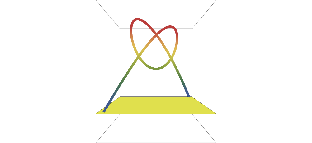
Figure 7. Long trefoil knot

Note that, the $z$ coordinate is zero exactly at two point corresponding to $t=-2.1554$ and $t=2.1554$.

Thus the spin construction will give us the map

$$(t,s)\to\big{(}x(t),y(t),z(t)\,Cos(s),z(t)\,Sin(s)\big{)}$$

giving the spun trefoil as the image. Now to obtain the polynomial map, we need to aproximate Cosine and Sine function in $[0,2\pi]$ using Chebyshev’s Polynomials. The Chebyshev approximaton of Cosine and Sine functions respectively are as follows.

$$C(s):= \,-0.0000193235s^{8}+0.000485652s^{7}-0.00399024s^{6}+0.0081095s^{5}$$

$$+0.0265068s^{4}+0.0163844s^{3}-0.509175s^{2}+0.00205416s+0.999921,$$

$$S(s):= \,8.73651067430188\times 10^{-19}s^{8}+0.000144829s^{7}-0.00318496s^{6}$$

$$+0.0220637s^{5}-0.0322337s^{4}-0.125592s^{3}-0.0257364s^{2}$$

$$+1.00614s-0.000238495.$$

Thus $(t,s)\to\big{(}x(t),y(t),z(t)\,C(s),z(t)\,S(s)\big{)}$ is a polynomial parametrization for the spun trefoil knot.
A Mathematica plot of its projection on xzw-plane, i.e.,

$$\Big{\{}\big{(}x(t),z(t)\,C(s),z(t)\,S(s)\big{)}\,\Big{|}\,t\in[-2.1554,2.1554],s\in[0,2\pi]\Big{\}}$$

and a hyperplane cross-sectional view are shown in Figure 8 and Figure 9 respectively.

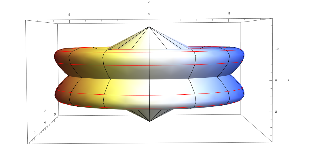
Figure 8. Projection of Spun trefoil on xzw-plane

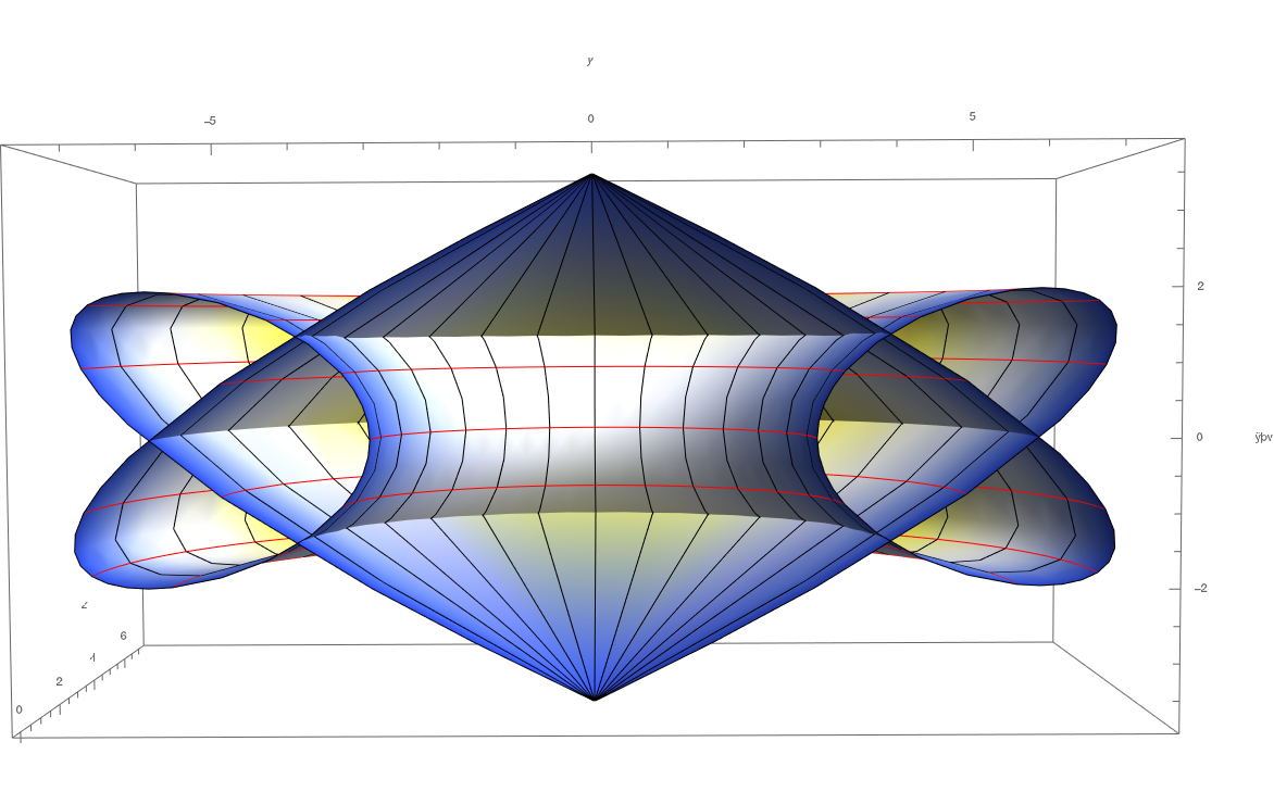
Figure 9. A cross-sectional view of Spun trefoil knot

1. Spun figure eight knot: Using the parametrization for long figure eight knot given in [3] and following the same procedure as above we obtain a polynomial parametrization of the spun figure eight knot by $(t,s)\to(x(t),y(t),z(t)\,C(s),z(t)\,S(s)\,)$ where,

$$x(t) =\frac{2}{5}\left(t^{2}-7\right)\left(t^{2}-10\right)t,$$

$$y(t) =\frac{1}{10}t\left(t^{2}-4\right)\left(t^{2}-9\right)\left(t^{2}-12\right),$$

$$z(t)\,C(s) =(20-13t^{2}-t^{4})\,(-0.0000193235s^{8}+0.000485652s^{7}-0.00399024s^{6}$$

$$+0.0081095s^{5}+0.0265068s^{4}+0.0163844s^{3}-0.509175s^{2}$$

$$+0.00205416s+0.999921\,),$$

$$z(t)\,S(s) =(20-13t^{2}-t^{4})\,(8.73651067430188\times 10^{-19}s^{8}+0.000144829s^{7}$$

$$-0.00318496s^{6}+0.0220637s^{5}-0.0322337s^{4}-0.125592s^{3}$$

$$-0.0257364s^{2}+1.00614s-0.000238495\,).$$

Figure 10 (b) and Figure 11 represent their projection on xzw-plane and a hyperplane cross-sectional view respectively.

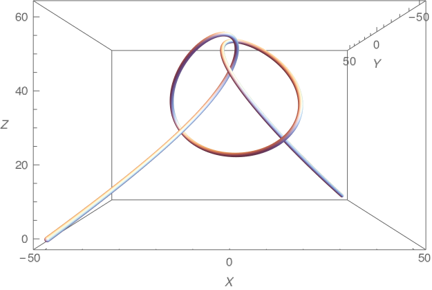
(a) long figure eight knot

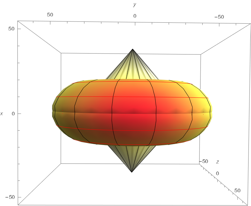
(b) Spun figure eight knot

Figure 10.

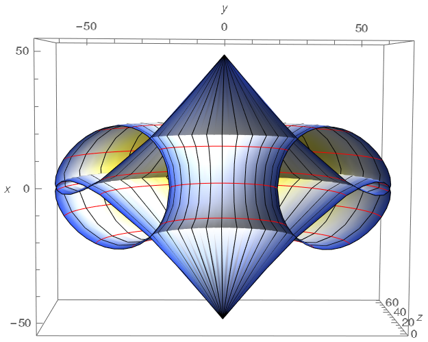
Figure 11. cross-sectional view of spun figure eight knot

4.2. Twist spun knots:

In order to polynomially parameterize twist spun of a knot $K$ we choose a polynomial parametrization for the classical long knot $K$ in $\mathbb{R}^{3}$,

$$K:\mathbb{R}\rightarrow\mathbb{R}^{3}$$

$$t\rightarrow\Big{\{}f(t),g(t),h(t)\Big{\}}$$

and consider a properly embedded arc which is the image of $K(t)$ for $t\in[a,b]$ i.e $k$ is embedded in $\mathbb{R}^{3}_{+}$ locally flatly and intersects $\partial\mathbb{R}^{3}_{+}$ transversely only at the endpoints $(f(a),g(a),0)$ and $(f(b),g(b),0)$. Now we can find an interval $[a^{\prime},b^{\prime}]\subset[a,b]$ where all the crossings of $K$ will lie.

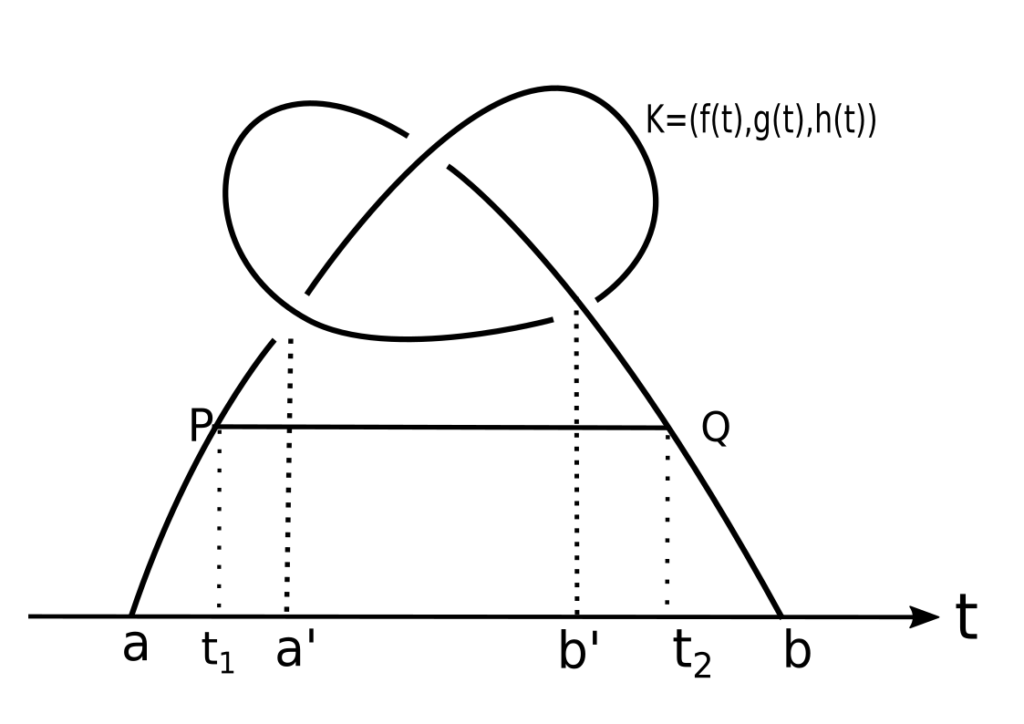
Figure 12. Rotating about $PQ$

To get a twist we choose the axis of rotation as a line segment $PQ$ parallel to the xy plane, joining two points on the knotted arc, say $P:=(f(t_{1}),g(t_{1}),h(t_{1}))$ and $Q:=(f(t_{2}),g(t_{2}),h(t_{2}))$ , where $[a^{\prime},b^{\prime}]\subset[t_{1},t_{2}]$ and $h(t_{1})=h(t_{2})=c$. We have to choose $c$ in such a way that the knotted part of the arc does not cross xy plane while rotating about $PQ$. Now, we will spin $K$ about xy plane while rotating about $PQ$ to get the twist spun knot. See Figure 12.
The rotation matrix around $PQ$ will be,

$$\mathbf{R}^{\prime}=\mathbf{T_{c}*R*T_{c}^{-1}}=\mathbf{T_{c}*R*T_{-c}},$$

where $\mathbf{T_{c}}$ is the translation matrix along z axis which will send $(x,y,z)$ to $(x,y,z+c)$ and $\mathbf{R}$ gives the rotation about the line $P^{\prime}Q^{\prime}$ on xy plane, parallel to $PQ$, joining the points $P^{\prime}=(f(t_{1}),g(t_{1}),0)$ and $Q^{\prime}=(f(t_{2}),g(t_{2}),0)$ on the knotted arc.

The matrix $\mathbf{R}$ is given by Rodrigues’ Rotation formula [13], which is described as follows: If $\mathbf{v}$ is a vector in $\mathbb{R}^{3}$ and $\mathbf{k}$ is a unit vector describing an axis of rotation about which $\mathbf{v}$ rotates by an angle $\phi$ according to the right hand rule, the Rodrigues formula for the rotated vector $\mathbf{v_{rot}}$ is given by

$$\mathbf{v}_{rot}=\mathbf{v}\,Cos\phi+(\mathbf{k}\times\mathbf{v})Sin\phi+\mathbf{k}\cdot(\mathbf{k}\cdot\mathbf{v})(1-Cos\phi)$$

In this situation $\mathbf{k}$ is along the line joining $(f(t_{1}),g(t_{1}),0)$ and $(f(t_{2}),g(t_{2}),0)$. So,

$$\mathbf{k}=\Big{(}\frac{f(t_{2})-f(t_{1})}{N},\frac{g(t_{2})-g(t_{1})}{N},0\Big{)},$$

where $N=\sqrt{(f(t_{2})-f(t_{1}))^{2}+(g(t_{2})-g(t_{1}))^{2}}.$

For simplification, denote

$$f(t_{2})-f(t_{1}):=f_{21}$$

$$g(t_{2})-g(t_{1}):=g_{21}$$

Then,

$$\mathbf{k}=\Big{(}\frac{f_{21}}{N},\frac{g_{21}}{N},0\Big{)},$$

where $N=\sqrt{f_{21}^{2}+g_{21}^{2}}.$

Then the rotation matrix through an angle $\phi$ counterclockwise about the axis $k$ is

$$\mathbf{R=I+Sin\phi\;K+(1-Cos\phi)\;K^{2}}$$

where,

$$\mathbf{K}= \begin{pmatrix}0&-k_{z}&k_{y}\\ k_{z}&0&-k_{x}\\ -k_{y}&k_{x}&0\end{pmatrix}$$

$$= \begin{pmatrix}0&0&\dfrac{g_{21}}{N}\\[14.22636pt] 0&0&-\dfrac{f_{21}}{N}\\[14.22636pt] -\dfrac{g_{21}}{N}&\dfrac{f_{21}}{N}&0\end{pmatrix}.$$

So, in our case

$$\mathbf{R}=\begin{pmatrix}\dfrac{f_{21}^{2}\;+\;g_{21}^{2}\;Cos\phi}{N^{2}}&\dfrac{f_{21}\;g_{21}\;(1-Cos\phi)}{N^{2}}&\dfrac{g_{21}\;Sin\phi}{N}\\[14.22636pt] \dfrac{f_{21}\;g_{21}\;(1-Cos\phi)}{N^{2}}&\dfrac{f_{21}^{2}\;Cos\phi\;+\;g_{21}^{2}}{N^{2}}&-\dfrac{f_{21}\;Sin\phi}{N}\\[14.22636pt] -\dfrac{g_{21}\;Sin\phi}{N}&\dfrac{f_{21}\;Sin\phi}{N}&Cos\phi\end{pmatrix}$$

Thus the rotation matrix about $PQ$ will be,

$$\mathbf{R}^{\prime}=\mathbf{T_{c}*R*T_{c}^{-1}}=\mathbf{T_{c}*R*T_{-c}},$$

where

$$\mathbf{R}=\begin{pmatrix}\dfrac{f_{21}^{2}\;+\;g_{21}^{2}\;Cos\phi}{N^{2}}&\dfrac{f_{21}\;g_{21}\;(1-Cos\phi)}{N^{2}}&\dfrac{g_{21}\;Sin\phi}{N}&0\\[14.22636pt] \dfrac{f_{21}\;g_{21}\;(1-Cos\phi)}{N^{2}}&\dfrac{f_{21}^{2}\;Cos\phi\;+\;g_{21}^{2}}{N^{2}}&-\dfrac{f_{21}\;Sin\phi}{N}&0\\[14.22636pt] -\dfrac{g_{21}\;Sin\phi}{N}&\dfrac{f_{21}\;Sin\phi}{N}&Cos\phi&0\\[14.22636pt] 0&0&0&1\end{pmatrix}$$

and $\mathbf{T_{c}}$ is the translation matrix along z axis which will send $(x,y,z)$ to $(x,y,z+c)$ given by

$$T_{c}=\begin{pmatrix}1&0&0&0\\ 0&1&0&0\\ 0&0&1&c\\ 0&0&0&1\end{pmatrix}.$$

Then,

$$\mathbf{R}^{\prime}=\begin{pmatrix}\dfrac{f_{21}^{2}\;+\;g_{21}^{2}\;Cos\phi}{N^{2}}&\dfrac{f_{21}\;g_{21}\;(1-Cos\phi)}{N^{2}}&\dfrac{g_{21}\;Sin\phi}{N}&-\dfrac{c\;g_{21}\;Sin\phi}{N}\\[14.22636pt] \dfrac{f_{21}\;g_{21}\;(1-Cos\phi)}{N^{2}}&\dfrac{f_{21}^{2}\;Cos\phi\;+\;g_{21}^{2}}{N^{2}}&-\dfrac{f_{21}\;Sin\phi}{N}&\dfrac{c\;f_{21}\;Sin\phi}{N}\\[14.22636pt] -\dfrac{g_{21}\;Sin\phi}{N}&\dfrac{f_{21}\;Sin\phi}{N}&Cos\phi&-c\;Cos\phi+c\\[14.22636pt] 0&0&0&1\end{pmatrix}.$$

This rotation about $PQ$ is given by the parametrization :

$$(t,\phi)\longrightarrow\left\{\big{(}f^{\prime}(t,\phi),g^{\prime}(t,\phi),h^{\prime}(t,\phi)\big{)}\,\middle|\,\begin{aligned} a\leq&t\leq b\\ 0\leq&\phi<2\pi\end{aligned}\,\right\}$$ (1)

where

$$f^{\prime}(t,\phi) :\frac{\big{(}f_{21}^{2}\;+\;g_{21}^{2}\;Cos\phi\big{)}\,\mathbf{f(t)}+f_{21}\;g_{21}\;(1-Cos\phi)\,\mathbf{g(t)}+N\;g_{21}\,Sin\phi\,(\mathbf{h(t)}-c)}{N^{2}}$$ (2)

$$g^{\prime}(t,\phi) :\frac{f_{21}\;g_{21}\;(1-Cos\phi)\,\mathbf{f(t)}+\big{(}f_{21}^{2}\;Cos\phi\;+\;g_{21}^{2}\big{)}\,\mathbf{g(t)}+N\;g_{21}\,Sin\phi\,(c-\mathbf{h(t)})}{N^{2}}$$ (3)

$$h^{\prime}(t,\phi) :\frac{-g_{21}\;Sin\phi\;\mathbf{f(t)}+f_{21}Sin\phi\;\mathbf{g(t)}+N\,Cos\phi\,\mathbf{h(t)}+N\,c\,(1-Cos\phi)}{N}$$ (4)

where, $N=\sqrt{f_{21}^{2}+g_{21}^{2}}.$

Now, the only thing to take care is that there should be no rotation outside the endpoints of the axis. We will achieve this by multiplying it with a bump function.
Construction of the bump function: To define the bump function $B(t)$, we first define the function $F(t)$ as :

$$F(t)=\begin{cases}e^{-\frac{1}{t}},&t>0\\ 0,&t\leq 0\end{cases}$$

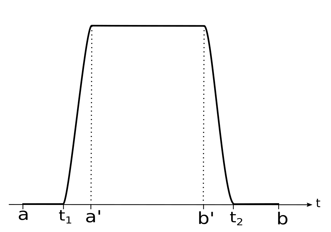
Figure 13. Constructing bump function

Then the $B(t)$ is defined as follows:

$$B(t)=\frac{F(d_{2}-t^{2})}{F(t^{2}-d_{1})+F(d_{2}-t^{2})}$$

where, we will choose $d_{1},d_{2}\in\mathbb{R}^{+}$ in such way that

$$B(t)=\begin{cases}1,&t\in[a^{\prime},b^{\prime}]\qquad\text{(which contains all crossings)}\\ 0,&t\in[a,t_{1}]\cup[t_{2},b]\\ \in(0,1),&\text{otherwise}\end{cases}$$

See Figure 13. Then, in $[a,b]$ define

$$\tilde{f}(t,\phi)= \,B(t)\,f^{\prime}(t,\phi)+(1-B(t))\,f(t)$$

$$\tilde{g}(t,\phi)= \,B(t)\,g^{\prime}(t,\phi)+(1-B(t))\,g(t)$$

$$\tilde{h}(t,\phi)= \,B(t)\,h^{\prime}(t,\phi)+(1-B(t))\,h(t)$$

Now,we will spin it about $xy$ plane in $\mathbb{R}^{4}$ while rotating about $PQ$ in $\mathbb{R}^{3}$ to get a twist spun knot. Then the rotation angle about $PQ$, $\phi=k\,\theta$, where $\theta$ will be the spinning angle about xy plane.
Hence,the parametrization for k-twist spun knot will be

$$(t,\theta)\longrightarrow\left\{\big{(}\tilde{f}(t,k\theta)\,,\,\tilde{g}(t,k\theta)\,,\,\tilde{h}(t,k\theta)\,Cos\,\theta\,,\,\tilde{h}(t,k\theta)\,Sin\,\theta\big{)}\,\middle|\,\begin{aligned} a\leq&t\leq b\\ 0\leq&\theta<2\pi\end{aligned}\right\}$$ (5)

Now, $\tilde{f},\tilde{g},\tilde{h}$ are linear combinations of the functions $f,g,h$ ,Cosine and Sine. Replacing Cosine and Sine functions with their corresponding Chebyshev polynomial approximation in $[0,2\pi]$, we obtain a polynomial parametrization of twist spun knots.

Example: Twist spun trefoil
As in the earlier example, we start with the following polynomial representation of trefoil knot:

$$x(t) :t^{3}-3t$$

$$y(t) :t^{5}-10t$$

$$z(t) :-t^{4}+4t^{2}+16$$

Here,

$$[a,b] =[-2.54404,2.54404]$$

$$[a^{\prime},b^{\prime}] =[-1.946,1.946]$$

$$P =(f[-2.19],g[-2.19],h[-2.19])$$

$$Q =(f[2.19],g[2.19],h[2.19])$$

$$c =h[2.19]$$

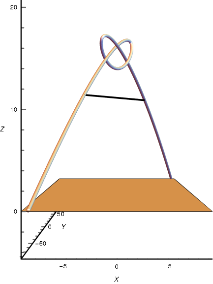
Figure 14. knotted trefoil arc with endpoints on $xy$ plane with axis of rotation

Hence, $\mathbf{k}$ is along the line joining $(-f[2.19],-g[2.19],0)$ and $(f[2.19],g[2.19],0)$.
So,

$$\mathbf{k}=\Big{(}\frac{f[2.19]}{\sqrt{f[2.19]^{2}+g[2.19]^{2}}},\frac{g[2.19]}{\sqrt{f[2.19]^{2}+g[2.19]^{2}}},0\Big{)}.$$

and

$$N=\sqrt{f[2.19]^{2}+g[2.19]^{2}}$$

This rotation about $PQ$ is given by the parametrization (See Figure 15) :

$$(t,\phi)\longrightarrow\left\{\big{(}f^{\prime}(t,\phi),g^{\prime}(t,\phi),h^{\prime}(t,\phi)\big{)}\;\middle|\;\begin{aligned} a\leq&t\leq b\\ 0\leq&\phi<2\pi\end{aligned}\,\right\}$$

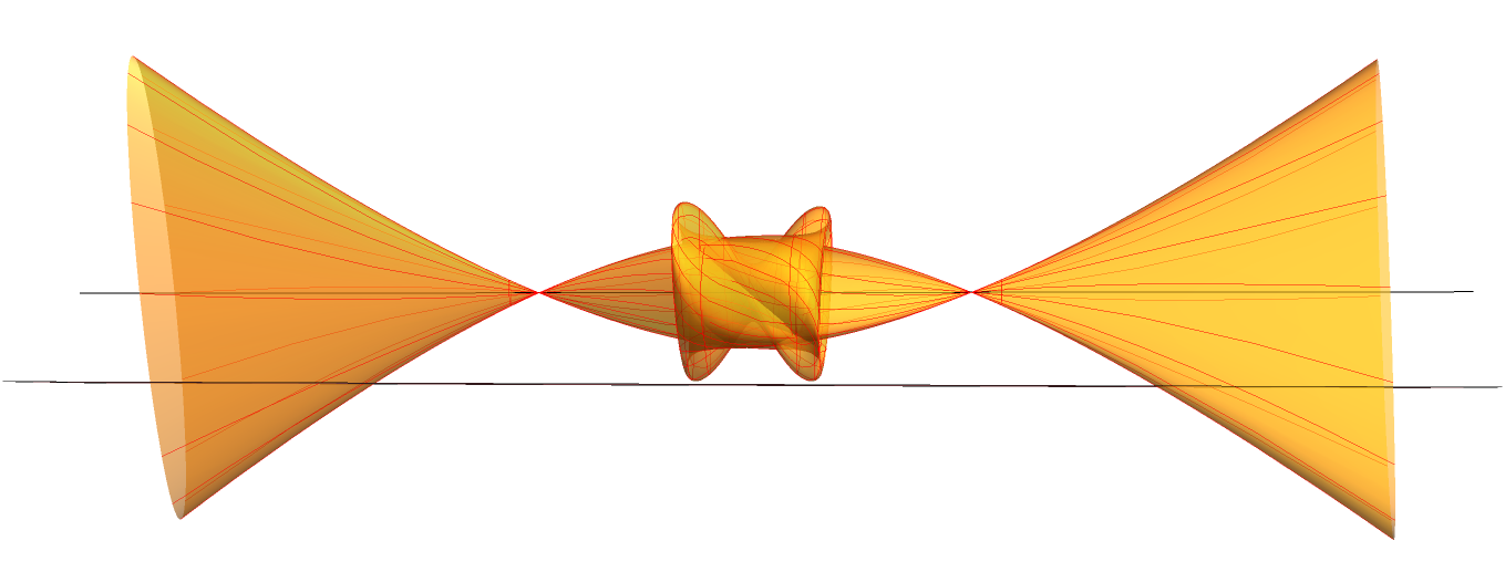
Figure 15. Rotating the long trefoil arc about $PQ$

where,

$$f^{\prime}(t,\phi) :\frac{\displaystyle\begin{multlined}\big{(}f[2.19]^{2}\;+\;g[2.19]^{2}\;Cos\phi\big{)}\,\mathbf{f(t)}+f[2.19]\;g[2.19]\;(1-Cos\phi)\,\mathbf{g(t)}\\ +(\mathbf{h(t)}-c)N\;g[2.19]\;Sin\phi\end{multlined}\big{(}f[2.19]^{2}\;+\;g[2.19]^{2}\;Cos\phi\big{)}\,\mathbf{f(t)}+f[2.19]\;g[2.19]\;(1-Cos\phi)\,\mathbf{g(t)}\\ +(\mathbf{h(t)}-c)N\;g[2.19]\;Sin\phi}{N^{2}}$$ (8)

$$g^{\prime}(t,\phi) :\frac{\displaystyle\begin{multlined}f[2.19]\;g[2.19]\;(1-Cos\phi)\,\mathbf{f(t)}+\big{(}f[2.19]^{2}\;Cos\phi\;+\;g[2.19]^{2}\big{)}\,\mathbf{g(t)}\\ +(c-\mathbf{h(t)})N\;g[2.19]\;Sin\phi\end{multlined}f[2.19]\;g[2.19]\;(1-Cos\phi)\,\mathbf{f(t)}+\big{(}f[2.19]^{2}\;Cos\phi\;+\;g[2.19]^{2}\big{)}\,\mathbf{g(t)}\\ +(c-\mathbf{h(t)})N\;g[2.19]\;Sin\phi}{N^{2}}$$ (11)

$$h^{\prime}(t,\phi) :\frac{-g[2.19]\;Sin\phi\;\mathbf{f(t)}+f[2.19]Sin\phi\;\mathbf{g(t)}+N\,\mathbf{h(t)}Cos\phi+N\,c\,(1-Cos\phi)}{N}$$ (12)

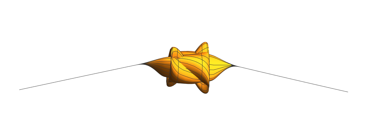
Figure 16. $(\tilde{f}(t,\phi),\tilde{g}(t,\phi),\tilde{h}(t,\phi))$ in $[-2.54404,2.54404]$

We define the bump function as:

$$B(t)=\frac{F(4.8-t^{2})}{F(t^{2}-3.8)+F(4.8-t^{2})}$$

The restricted rotation about $PQ$ (See Figure 16 ) is given by

$$(t,\theta)\longrightarrow\left\{\big{(}\tilde{f}(t,\phi),\tilde{g}(t,\phi),\tilde{h}(t,\phi)\big{)}\,\middle|\,\begin{aligned} -2.54404\leq&t\leq 2.54404\\ 0\leq&\phi<2\pi\end{aligned}\right\}$$

where,

$$\begin{aligned} \tilde{f}(t,\phi)=&\,B(t)\,f^{\prime}(t,\phi)+(1-B(t))\,f(t)\\ \tilde{g}(t,\phi)=&\,B(t)\,g^{\prime}(t,\phi)+(1-B(t))\,g(t)\\ \tilde{h}(t,\phi)=&\,B(t)\,h^{\prime}(t,\phi)+(1-B(t))\,h(t)\end{aligned}$$ (13)

.

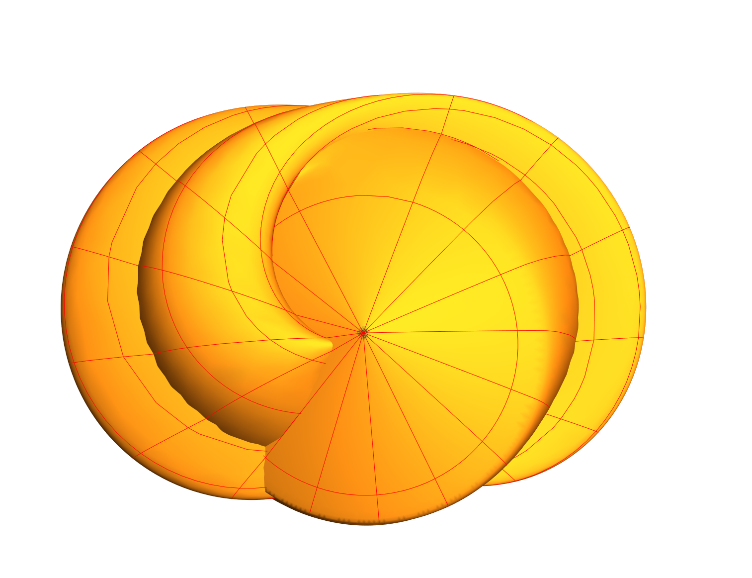
(a) Top view

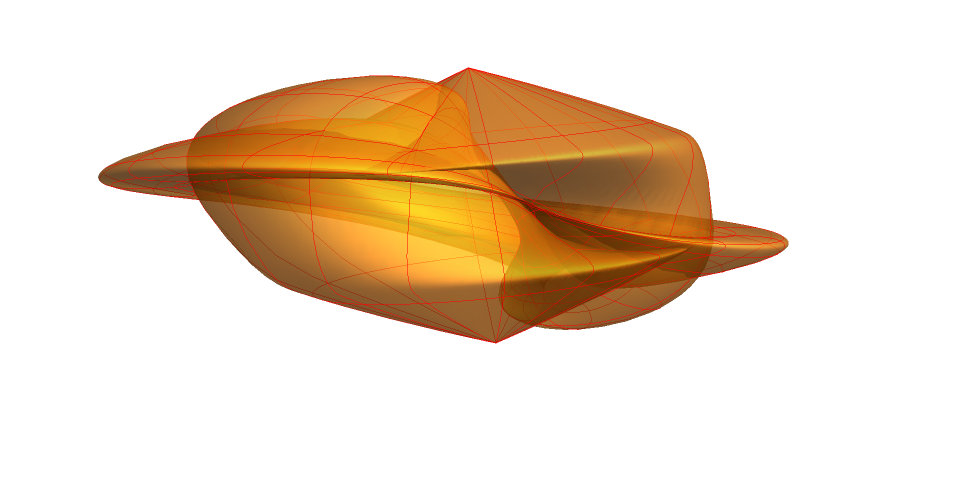
(b) Side view

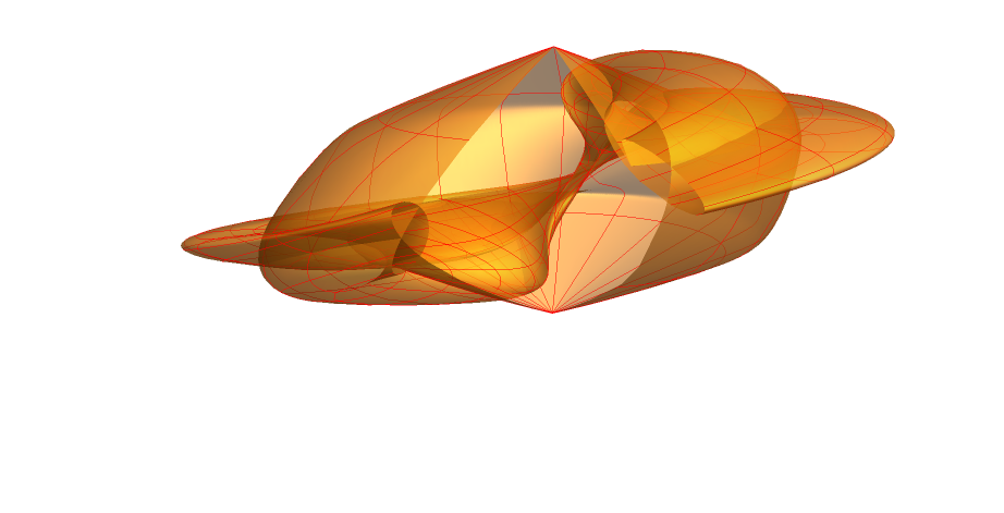
(c) $0\leq\theta\leq\frac{3\pi}{2}$

Figure 17. Projection of 1-twist spun trefoil in $\mathbb{R}^{3}$

Hence,the parametrization for k-twist spun trefoil knot will be

$$(t,\theta)\longrightarrow\left\{\big{(}\tilde{f}(t,k\theta),\tilde{g}(t,k\theta),\tilde{h}(t,k\theta)\,Cos\theta,\tilde{h}(t,k\theta)\,Sin\theta\big{)}\;\middle|\;\begin{aligned} -2.54404\leq&t\leq 2.54404\\ 0\leq&\theta<2\pi\end{aligned}\right\}$$

Some projections of the k twist spun trefoil $\text{for}\,k=2,3,10$ in $\mathbb{R}^{3}$ are shown in Figures 18,19,20 respectively.

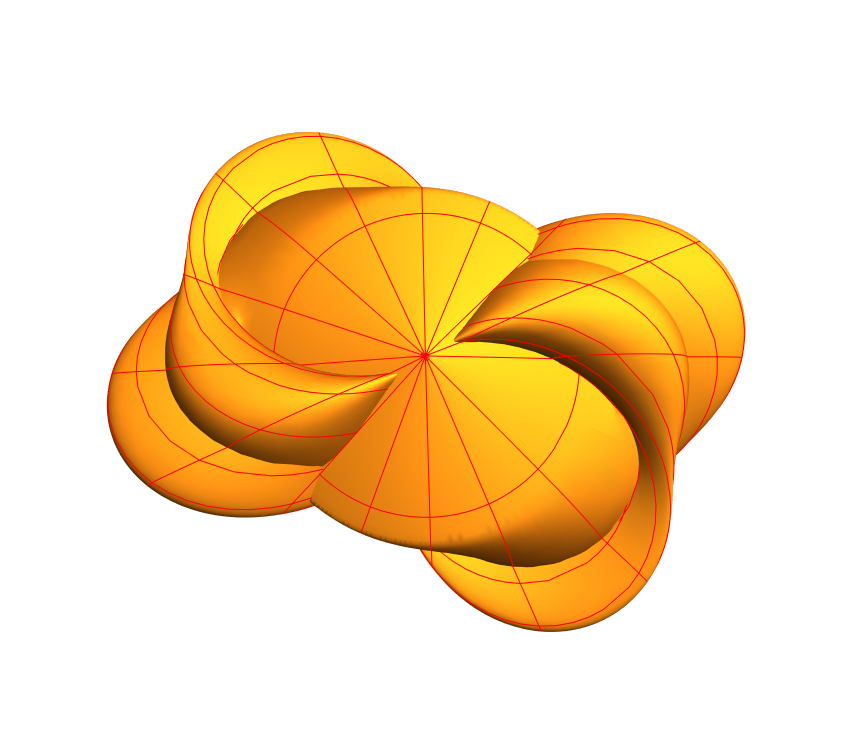
(a) Top view

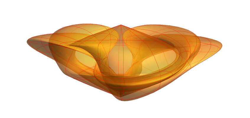
(b) Side view

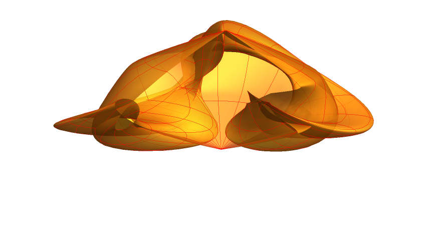
(c) $0\leq\theta\leq\frac{3\pi}{2}$

Figure 18. 2-twist spun trefoil

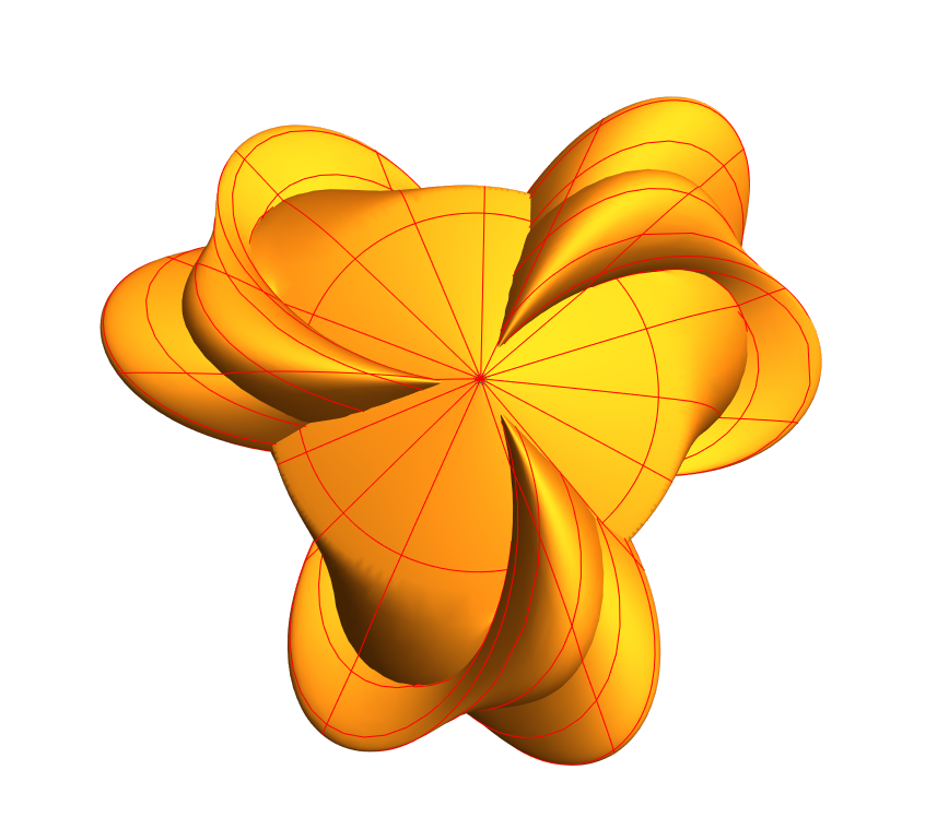
(a) Top view

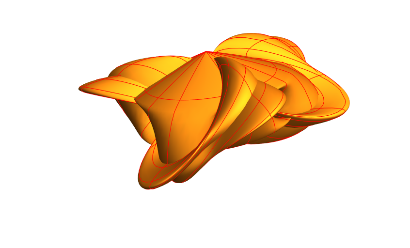
(b) Side view

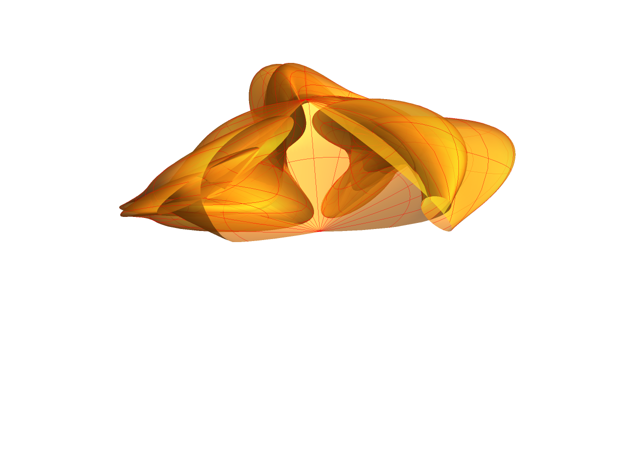
(c) $0\leq\theta\leq\frac{3\pi}{2}$

Figure 19. 3-twist spun trefoil

(a) Top view

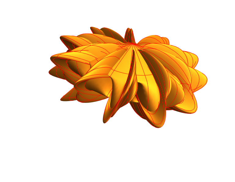
(b) Side view

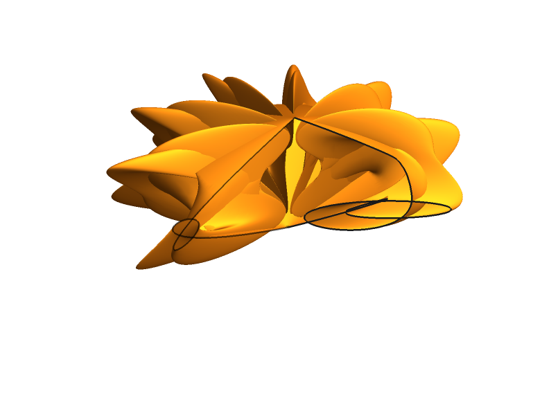
(c) $0\leq\theta\leq\frac{3\pi}{2}$

Figure 20. 10-twist spun trefoil

5. Conclusion:

A more general spinning construction is described by R.A.Litherland [7] called Deform Spinning, where roll-spun knot and twist-spun knots are special cases. We would like to find a way to parameterize these $2$ knots since these are obtained by deforming classical knotted arc using some transformations in $\mathbb{R}^{3}$ while spinning. Finding a general method to parameterize any $2$ knot will be a goal in the next project.

References

- [1] Abutheraa, M. A., Lester, D., & Ardil, C. (Ed.) (2007). Computable Function Representations Using Effective Chebyshev Polynomial. In C. Ardil (Ed.), Conference of the World-Academy-of-Science-Engineering-and-Technology (Vol. 25, pp. 103-109). World Academy of Science, Engineering and Technology.
- [2] Artin, E. (1925). Zur Isotopie zweidimensionaler Flächen imR4. Abhandlungen aus dem Mathematischen Seminar der Universität Hamburg, 4, 174-177.
- [3] Brown, A.N. (2004). Examples of polynomial knots.
- [4] Carter, J.S., & Saito, M. (1997). Knotted Surfaces and Their Diagrams.
- [5] Durfee, A., & O’Shea, D. (2006). Polynomial knots. arXiv preprint math/0612803.
- [6] Gluck, H. (1961). THE EMBEDDING OF TWO-SPHERES IN THE FOUR-SPHERE. Bulletin of the American Mathematical Society, 67, 586-589.
- [7] R.A. Litherland, Deforming twist-spun knots, Trans. Amer. Math. Soc. 250 (1979), 311–331
- [8] Mishra, R., & M.Prabhakar (2008). Polynomial representation for long knots. arXiv: Geometric Topology.
- [9] Mishra, R. (2000). Minimal Degree Sequence for Torus Knots. Journal of Knot Theory and Its Ramifications, 09, 759-769..”
- [10] Shastri A.R,Polynomial Representation of knots, Tohoku Math. J. (2) 44 (1992) 11-17.
- [11] Shukla, R. On polynomial isotopy of knot-types. Proc. Indian Acad. Sci. (Math. Sci.) 104, 543–548 (1994).
- [12] Kamada, S. (2002). Braid and Knot Theory in Dimension Four.
- [13] Rodrigues, O. (1840). Des lois géométriques qui régissent les déplacements d’un système solide dans l’espace, et de la variation des coordonnées provenant de ces déplacements considérés indépendamment des causes qui peuvent les produire. Journal de mathématiques pures et appliquées, 5, 380-440.
- [14] Stancu, D. D. (1963). A Method for Obtaining Polynomials of Bernstein type of two Variables. The American Mathematical Monthly, 70(3), 260–264. https://doi.org/10.2307/2313121
- [15] Rudin, W. (1953). Principles of mathematical analysis, International Series of Pure and Applied Mathematics.
- [16] Zeeman, E.C. (1965). Twisting spun knots. Transactions of the American Mathematical Society, 115, 471-495.