Multimodal Motion Conditioned Diffusion Model for Skeleton-based Video Anomaly Detection

Abstract

Anomalies are rare and anomaly detection is often therefore framed as One-Class Classification (OCC), i.e. trained solely on normalcy. Leading OCC techniques constrain the latent representations of normal¹ motions to limited volumes and detect as abnormal anything outside, which accounts satisfactorily for the openset’ness of anomalies. But normalcy shares the same openset’ness property since humans can perform the same action in several ways, which the leading techniques neglect.

We propose a novel generative model for video anomaly detection (VAD), which assumes that both normality and abnormality are multimodal. We consider skeletal representations and leverage state-of-the-art diffusion probabilistic models to generate multimodal future human poses. We contribute a novel conditioning on the past motion of people and exploit the improved mode coverage capabilities of diffusion processes to generate different-but-plausible future motions. Upon the statistical aggregation of future modes, an anomaly is detected when the generated set of motions is not pertinent to the actual future. We validate our model on 4 established benchmarks: UBnormal, HR-UBnormal, HR-STC, and HR-Avenue, with extensive experiments surpassing state-of-the-art results.

1 Introduction

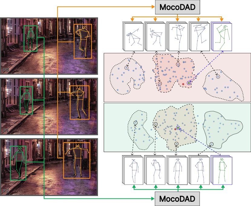
Figure 1: MoCoDAD detects anomalies by synthesizing and statistically aggregating multi-modal future motions, conditioned on past poses (frames on the left). Red (top) and green (bottom) distributions represent examples of anomaly and normality generations (2d mapped via t-SNE). Within the distribution modes (dashed-contoured), the red dots are the actual true futures corresponding to the conditioning past frames. In the case of normality, the true future lies within a main distribution mode, and the generated predictions are pertinent. In the case of abnormality, the true future lies in the tail of the distribution modes, which yields poorer predictions, highlighting anomalies.

Video Anomaly Detection (VAD) is a crucial task in computer vision and security applications. It enables early detection of unusual or abnormal events in videos, such as accidents, illnesses, or people’s behavior which may threaten public safety [45]. However, several aspects make VAD a challenging task. Firstly, the definition of anomaly is highly subjective and varies depending on the context and application, making it difficult to define it universally. Secondly, anomalies are intrinsically rare. To account for data scarcity, models generally learn from regular samples only (also known as One Class Classification - OCC) or have to cope with the data imbalance. Thirdly, anomaly detection is intrinsically an openset problem, and modeling anomalies needs to account for diversity beyond the training set.

An “ideal” model for anomaly detection should consider that there are infinitely many anomalous and non-anomalous ways of performing an action. Current state-of-the-art OCC techniques [9, 26, 27, 28] fail to address this issue. Indeed, they focus on learning either a single reconstruction or prediction of the input, or deriving a latent representation of normal actions, thereby constraining them to a limited latent volume. This last approach successfully accounts for the openset’ness of anomalies, i.e., anything mapped outside the normality region is considered abnormal. However, forcing normality into constrained volumes may not work for diverse-but-still-normal behaviors, i.e., OCC misclassifies as anomalous those not fitting in the volume.

We propose Motion Conditioned Diffusion Anomaly Detection - hereafter MoCoDAD - a novel generative model for VAD, which assumes that both normality and abnormality are multimodal. Given a motion sequence, be it normal or anomalous, the sequence is split and the later (future) frames are corrupted to become random noise. Conditioned on the first (past) clean input frames, MoCoDAD synthesizes multimodal reconstructions of the corrupted frames. MoCoDAD discerns normality from anomaly by comparing the multimodal distributions. In the case of normality, the generated motions are diverse but pertinent, i.e. they are biased towards the true uncorrupted frames. In the case of abnormality, the synthesized motion is also diverse, but it lacks pertinence, as shown in Fig. 1 and discussed in Sec. 5.

MoCoDAD is the first diffusion-based technique for video anomaly detection. We are inspired by Denoising Diffusion Probabilistic Models (DDPMs) [44, 15], state-of-the-art, among others, in image synthesis [35, 34, 37], motion synthesis [47, 54], and 3D generation tasks [59]. DDPMs are selected for their improved mode coverage [53], i.e. they generate diverse multimodal motions, which MoCoDAD statistically aggregates (see the respective ablative study in Sec. 5).

Besides multimodality, a crucial aspect of MoCoDAD is the choice of the conditioning strategy to guide the synthesis. We consider human motion as skeletal representations and propose corrupting the body joint coordinates at each frame by displacing them with random translations. Conditioning refers to the process that provides the model with the uncorrupted first part of the motion sequence (past) to guide the denoising of the corrupted second part (future). In this study, we compare three modeling choices to find the most suitable conditioning strategy. We experiment with (1) directly feeding the denoising module with the concatenation of the uncorrupted poses with the displaced sequence [39]. For the other two strategies, we get a latent representation of the input (via (2) an encoding module and (3) an autoencoder) and feed the network with this learned representation (cf. Sec. 3.2). The third strategy works best (cf. Sec. 5.3).

We evaluate MoCoDAD on three challenging benchmarks of human-related anomalies, namely, HR-UBnormal [1, 9], HR-ShanghaiTech Campus [25, 28] (HR-STC), and HR-Avenue [24, 28], and on the most recent VAD dataset UBnormal [1]. MoCoDAD achieves state-of-the-art (SoA) performance on all four datasets, which demonstrates the effectiveness of modeling multimodality for normal and abnormal motions. Notably, by not using appearance, MoCoDAD benefits increased privacy protection (no visual facial nor body features) and better computational efficiency, thanks to the lightweight body kinematic representations. We summarize our contributions as follows:

• A novel generative VAD model based on comparing the multimodality of normal and abnormal motion generations;

• The first probabilistic diffusion-based approach for VAD, which fully exploits the enhanced mode-coverage capabilities of diffusive probabilistic models;

• A novel motion-based conditioning on the clean input sequence to steer the synthesis towards diverse pertinent motion in the case of normality;

• A thorough validation on UBnormal, HR-UBnormal, HR-STC, and HR-Avenue benchmarks where we outperform the SoA by $5.1\%$, $4.4\%$, $.5\%$, $.8\%$, respectively.

2 Related Work

Previous work relates to ours from two main perspectives: Video Anomaly Detection methods (see Sec. 2.1), and diffusion models for motion synthesis (see Sec. 2.2).

2.1 Video Anomaly Detection Techniques

Pioneer works analyze the trajectory of the agents in the frames to discriminate those distant from normality [5, 17, 21]. Within recent literature, two major trends can be identified: latent- and reconstruction-based methods. VAD techniques also vary based on the type of input data they use, such as videos or human skeletal pose motions. MoCoDAD, as all the VAD works presented in this section, adheres to the OCC protocol, which simulates the scarcity of anomalies in real-world scenarios [19].

Latent-based VAD methods identify abnormality according to a score extracted from a learned latent space whereby normality is supposedly mapped into a constrained volume, and anomalies are those latents lying outside, with a larger score (see [38, 42, 46, 51] for an overview of latent-based AD). Sabokrou et al. [40] propose a two-staged cascade of deep neural networks. First, they employ a stack of autoencoders that detects points of interest (POIs) while excluding irrelevant patches (e.g., background). Second, they identify anomalies by densely extracting and modeling discriminative patches at POIs. Notice that this work constrains normality to belong to a single mode and anomalies outside, thus, addressing the openset’ness of anomalies, but it hampers the multimodal and diversity [57] aspect of normal motions. Contrarily, our work considers the multimodality of normal and abnormal motions.

Notably, Nguyen et al. [29] propose an image-based technique exploring multimodal anomaly detection via multi-headed VAEs. However, considering a fixed number of modes for reality amends multimodality only partially, as it misses to unleash its openset’ness. Differently, we adopt diffusion models for their improved mode coverage and generate multiple futures, not being constrained on a fixed number of heads (see Sec. 5).

Reconstruction-based VAD methods consider the original metric space of the input and leverage reconstruction as the proxy task to derive an anomaly score. These models are trained to encode and reconstruct the input from normal events, producing larger errors on anomalies not seen during training. [7, 14, 58] use sequences of frames and feed them to convolutional autoencoders. Gong et al. [12] “memorize” the most representative normal poses to discriminate new input samples. Liu et al. [23] tackle intensity and gradient loss, optical flow, and adversarial training. Luo et al. [25] use stacked RNNs with temporally-coherent sparse coding enforcing similar neighboring frames to be encoded with similar reconstruction coefficients. Barbalau et al. [3] builds upon [10] and integrates the reconstruction of the input frames, via multi-headed attention, into a multi-task learning framework. Besides [10, 23], all works rely on a single reconstruction proxy task via non-variational architectures that learn discrete manifolds. However, normality and abnormality are multimodal and diverse, making it hard for these techniques to have an exact match (reconstruction) over the GT. Additionally, GANs used in [23] suffer from mode collapse [48] lacking to represent the multimodality of reality. Similarly to [29], [3] can represent only a fixed number of modalities, which does represent the openset’ness of reality. MoCoDAD is a reconstruction-based approach and leverages diffusion processes [8] to account for the openset’ness of normalcy and anomalies in terms of pertinence to the GT.

Skeleton-based VAD methods exploit compact spatio-temporal skeletal representations of human motion instead of raw video frames. Morais et al. [28] use two GRU autoencoder branches to account for the global and local decomposition of the skeleton in a particular frame. Luo et al. [26] exploit stacked layers of ST-GCN [55] to accumulate joint information over the spatio-temporal dimensions of the frame and predict joints in the future. However, [55] uses a fixed adjacency matrix, depicting joint connections, for all ST-GCN layers, which hinders the exploration of intra-frame and intra-joint relationships, two factors that play a crucial role in improving the encoding of spatio-temporal features [43]. Markovitz et al. [27] utilize the encoder of an ST-GCN autoencoder to embed space-time skeletons into a latent vector. This vector is then fed to an end-to-end trainable deep-embedded clustering procedure which produces $k$ clusters representing the multimodality of normalcy and anomalies. Flaborea et al. [9] propose COSKAD and force the normal instances into the same latent region driving the distances to a common center. MoCoDAD is also a skeleton-based approach that mitigates the choice of $k$ a priori to cover the multimodality of reality.

2.2 Diffusion Models

Diffusion models have marked a revolution in generative tasks such as image and video synthesis [39, 47, 54], but they have not been employed for VAD. Saadatnejad et al. [39] propose a two-step framework based on temporal cascaded diffusion (TCD). First, they denoise imperfect observation sequences and, then, improve the predictions of the (frozen) model on repaired frames. Tevet et al. [47] use a transformer encoder to learn arbitrary length motions [2, 33] coherent with a particular conditioning signal $c$. They experiment with constrained synthesis where $c$ is a text prompt (i.e., text-to-motion) or a specific action class (i.e., action-to-motion) and unconstrained synthesis where $c$ is not specified. Chen et al. [54] design a transformer-based VAE [33] to learn a representative latent space for human motion sequences. They apply a diffusion model in this latent space to generate vivid motion sequences while obeying specific conditions similar to [47]. Differently, MoCoDAD is a diffusion-based model that uses conditioning over a portion of the input (e.g., previous frames condition the generation of future ones).

Wyatt et al. [52] propose AnoDDPM, a diffusion model on images, which does not require the entire Markov chain (noise/denoise) to take place. They use decaying octaves of simplex noising functions to distinguish the corruption rate of low-frequency components from high-frequency ones. However, they add and remove noise without conditioning, identifying anomalies when noise removal diverges from the input. Differently, MoCoDAD is based on generating and comparing multimodal motions against the GT in terms of pertinence. Our proposed model is the first to exploit the multimodal generative and improved mode-coverage capabilities of diffusive techniques, via forecasting tasks, further to being first in adopting them for detecting video anomalies. Hence, to transfer DDPMs from video-based Anomaly Detection to skeleton-based VAD we rely on a U-Net-shaped stack of STS-GCN [43, 41] layers, which includes the spatio-temporal aspects of joints in sequences of human poses.

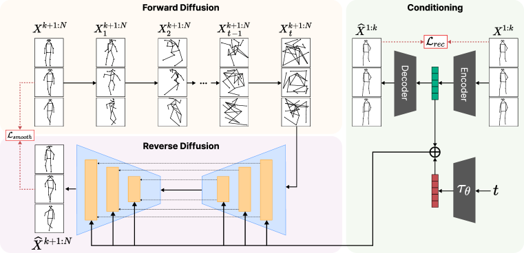
Figure 2: Overview of the proposed MoCoDAD. A sequence of $N$ skeletal motions ($N=6$ in the example) is split into past (top-right $X^{1:k}$ frames, $k=3$ in the example) and future (top-left $X^{k+1:N}$ frames). During training, the Forward Diffusion block adds noise to the future frames, shifting each joint by a random vector displacement of varying intensity (increasing with the diffusion timestep $t$). Then the Reverse Diffusion learns to estimate the noise. A key aspect of MoCoDAD is the conditioning, i.e. how to encode the past clean $k$ frames and guide the synthesis of relevant futures.

3 Methodology

MoCoDAD learns to reconstruct the later (future) corrupted poses by conditioning on the first (past) poses. Sec. 3.1 describes the training diffusion denoising process, how it generates multimodal reconstructions, and statistically aggregates them at inference to detect anomalies. Sec. 3.2 details conditioning on past frames, and Sec. 3.3 describes the architecture of MoCoDAD. For the sake of completeness, in Sec. A.1 of the Supplementary, we present preliminary concepts of DDPMs. Further, in Sec. C of the Supplementary we provide the pseudocode for training and evaluating our proposed MoCoDAD.

3.1 Diffusion on Trajectories

Training

We define a diffusion technique that learns to reconstruct corrupted future motion sequences conditioned on clean past ones.

Let $X_{a}=\{x_{a}^{1},\ldots,x_{a}^{N}\}$ be a sequence of $N$ time-contiguous poses belonging to a single actor $a$. Since our model considers one actor at a time, we use $X=\{x^{1},\dots,x^{N}\}$ for notation simplicity. Each pose $x^{i}$ can be seen as a graph $x^{i}=(J,A)$ where $J$ represents the set of joints, and $A$ is the adjacency matrix representing the joint connections. Notice that each joint is attributed with a set of spatial coordinates in $\mathbb{R}^{C}$, hence $x^{i}\in\mathbb{R}^{|J|\times C}$, and $X\in\mathbb{R}^{N\times|J|\times C}$. Here, we use $C=2$ as the person’s pose is extracted from images at each frame.

We divide $X$ into two parts: the past $X^{1:k}$ and the future sequence of poses $X^{k+1:N}$ with $k\in\{1,...,N\}$ .

During the forward process $q$, we corrupt the coordinates of the joints by adding random translation noise. We sample a random displacement map $\varepsilon^{k+1:N}\in\mathbb{R}^{(N-k)\times|J|\times C}$ from a distribution $\mathcal{N}(0,\mathbf{I})$ and add it to $X^{k+1:N}$ to randomly translate the position of its nodes.

The magnitude of the added displacement depends on a variance scheduler $\beta_{t}\in(0,1)$ and a diffusion timestep $t\sim\mathcal{U}_{[1,T]}$. As a result, $q$ increasingly corrupts the joints $x^{i}$ at each diffusion timestep $t$ (i.e., $x_{t=1}^{i}\rightarrow\dots\rightarrow x_{t=T}^{i}$) making $x_{t=T}^{i}$ indistinguishable from a pose with randomly sampled joints’ spatial coordinates.

The reverse process $p_{\theta}$ unrolls the corruption, estimating the spatial displacement map $\varepsilon^{k+1:N}$ via a U-Net-like architecture $\varepsilon_{\theta}$ (see Sec. 3.3 for more details). To achieve an approximation of $\varepsilon^{k+1:N}$, we train the network conditioned on the diffusion timestep $t$ (embedded through an MLP $\uptau_{\theta}$) and the embedding $h$ of the previous trajectory $X^{1:k}$.

In Eq. 1, similarly to [37], we define the displacement estimation objective.

$$\mathcal{L}_{disp}={\mathbb{E}_{t,X,\varepsilon}}\bigg{[}\big{|}\big{|}\varepsilon-\varepsilon_{\theta}(X_{t},t,h)\big{|}\big{|}\bigg{]}$$ (1)

Inspired by [11], we smooth $\mathcal{L}_{disp}$ as follows:

$$\mathcal{L}_{smooth}=\begin{cases}0.5\cdot(\mathcal{L}_{disp})^{2}&\text{ if }|\mathcal{L}_{disp}|<1\\ |\mathcal{L}_{disp}|-0.5&\text{ otherwise}\end{cases}$$ (2)

Inference

At inference time, MoCoDAD generates multimodal future sequences of poses from random displacement maps, conditioned on the past frames, then aggregates them statistically to detect anomalies.

We sample a random displacement $z\sim\mathcal{N}(0,\textbf{I})$ and consider it the starting point of the synthesis process that generates a future human motion via Eq. 3.

$$X_{t-1}=\frac{1}{\sqrt{\alpha_{t}}}\bigg{(}X_{t}-\frac{1-\alpha_{t}}{\sqrt{1-\alpha_{t}}}\varepsilon_{\theta}(X_{t},t,h)\bigg{)}+z\sqrt{\beta_{t}}$$ (3)

Note the motion conditioning $h$, encoding the past $k$ frames. We generate $m$ diverse future pose trajectories $Z_{1},\dots,Z_{m}$. For each $Z_{i}$, we compute the reconstruction error via the smoothed loss $s_{i}=\mathcal{L}_{smooth}(|X-Z_{i}|)$ used in training (cf. Eq. 2).

We aggregate all the scores from the generations $S=\{s_{1},\dots,s_{m}\}$ to distill a single anomaly score for that sequence. This score is subsequently assigned to the corresponding frames to assess their level of anomaly. In scenarios where multiple actors occupy the same frames, we assign the average anomaly score to those frames. See the Supplementary for a detailed description. We explore different strategies for distilling the anomaly score from $S$: (1) the diversity between the normal and anomalous generations and (2) aggregation statistics. To account for diversity, we consider the diversity metric $rF=\mathrm{mean}(\mathcal{L}_{smooth})/\min{(\mathcal{L}_{smooth})}$ introduced by [6, 31]. Diversity stems from testing whether anomalous generations are more diverse than normals, but the diversity score fails to detect anomalies, nearly dropping to random chance. We explain this by normalcy and anomaly having a similar degree of diversity, as we experimentally validate in Sec. 5.1.

We consider as aggregation statistics the mean, quantile robust statistics including the median, as well as maximum and minimum selectors, in terms of $\mathcal{L}_{smooth}$ distances between the $m$ generated and the GT future motion. Our analysis highlights that the minimum distance is the best on average. This reinforces the original hypothesis that normality-conditioned generated motions are as diverse as abnormal-conditioned ones but more biased to the actual motion, thus more likely to generate samples close to it. See Sec. 5.2 for the experimental evaluation.

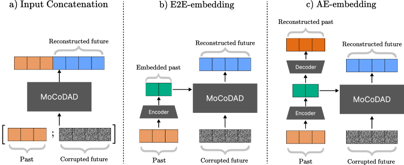
Figure 3: Comparison of the three conditioning strategies.

3.2 Motion Conditioning for multimodal Pose Forecasting

The choice of the conditioning strategy is a crucial factor for diffusion models, as it determines how the conditioning information is fed into the network, and it directly affects the quality of the outputs. In this work, we propose a thorough examination of different strategies for feeding the diffusion models with the conditioning information.

We identify three different modeling choices for conditioning the diffusion, illustrated in Fig. 3, i.e., input concatenation, E2E-embedding, and AE-embedding. Input concatenation refers to conditioning with a portion of the raw input motion. Here, we keep the past sequence of poses $X^{1:k}$ (the conditioning signal) uncorrupted and prepend it to the corrupted future sequence $X^{k+1:N}_{t}$. Input concatenation has been explored in previous work for pose forecasting reaching SoA performances in [39].

Table 1: Comparison of MoCoDAD against SoA in terms of AUC on the three Human-Related datasets (i.e., HR-STC, HR-Avenue and HR-UBnormal) and UBnormal. OCC skeleton-based techniques are marked with a $*$.

		HR-STC	HR-Avenue	HR-UBnormal	UBnormal
Conv-AE [14]	CVPR ’16	69.8	84.8	-	-
Pred [23]	CVPR ’18	72.7	86.2	-	-
MPED-RNN [28] $*$	CVPR ’19	75.4	86.3	61.2	60.6
GEPC [27] $*$	CVPR ’20	74.8	58.1	55.2	53.4
Multi-timescale Prediction [36] $*$	WACV ’20	77.0	88.3	-	-
Normal Graph [26]	Neurocomputing ’21	76.5	87.3	-	-
PoseCVAE [16] $*$	ICPR ’21	75.7	87.8	-	-
BiPOCO [18] $*$	Arxiv ’22	74.9	87.0	52.3	50.7
STGCAE-LSTM [22] $*$	Neurocomputing ’22	77.2	86.3	-	-
SSMTL++  [3]	CVIU ’23	-	-	-	62.1
COSKAD [9] $*$	Arxiv ’23	77.1	87.8	65.5	65.0
MoCoDAD $*$		77.6	89.0	68.4	68.3

Both embedding choices refer to passing the conditioning past frames through an encoder $E$, then providing them to all latent layers of the denoising model (cf. incoming vertical arrows into the orange layers in Fig. 2). Here, $E$ is a GCN [43] and it encodes sequences of poses $X^{1:k}$ into the representation $h=E(X^{1:k})$. In the case of E2E-embedding, $E$ is jointly learned with the rest of the architecture, leveraging the training $\mathcal{L}_{smooth}$ loss. The AE-embedding adds an auxiliary reconstruction loss $\mathcal{L}_{rec}$ to support training $E$, as it tasks a decoding network $D$ to reconstruct the conditioning past frames according to the following loss function:

$$\mathcal{L}_{rec}=\bigg{|}\bigg{|}D(E(X^{1:k}))-X^{1:k}\bigg{|}\bigg{|}^{2}_{2}$$ (4)

In the case of AE-embedding, the auxiliary is summed to the main loss, resulting in the following total loss:

$$\mathcal{L}_{tot}=\lambda_{1}\mathcal{L}_{smooth}+\lambda_{2}\mathcal{L}_{rec}$$ (5)

where $\lambda_{1}$,$\lambda_{2}\in[0,1]$ account for the contribution of each loss function respectively. Lastly, since DDPMs benefit from being conditioned on the timestep $t$, we add the embedding $\uptau_{\theta}(t)$ to the latent $h$ and feed the resulting motion-temporal signal to each layer of our network $\varepsilon_{\theta}$ [47].

The results of evaluation are discussed in Sec. 5.3, whereby applying an AE-embedding conditioning on $X^{1:k}$ emerges with results beyond the SoA.

3.3 Architecture Description

Fig. 2 illustrates the architecture of MoCoDAD. We distinguish two main blocks: a conditioning auto-encoder for the past motion, $X^{1:k}$, and a denoising model for $X^{k+1:N}$. The main diffusion model architecture is the neural network, represented with orange blocks, tasked with estimating the corrupting noise in the input motion, thus reconstructing the actual future motion. As done in [52], we rely on a U-Net like architecture. Our skeletal-motion diffusion network progressively contracts and then expands (rebuilds) the spatial dimension of the input sequence of poses. To account for the temporal dimension of the input sequences, we build the U-Net with space-time separable GCN (STS-GCN) layers proposed in [43]. The conditioning autoencoder relies on STS-GCN to reconstruct the past motion and embed it into a latent space used to condition the diffusion.

In detail, the U-Net takes in input $X^{k+1:N}$ and a motion-temporal conditioning signal $h+\uptau_{\theta}(t)$ which provides the network with the diffusion timestep and the encoded past-motion information. Furthermore, to align the dimensionality of this conditioning signal with that of the network’s layers, the former is fed into an embedding layer projecting it to the correct vector space. This embedded conditioning signal is then fed to each STS-GCN layer. The contracting process of the U-Net progressively aggregates the joints of the poses (i.e., $\mathbb{R}^{J}\rightarrow\mathbb{R}^{d}\text{ s.t. }d\leq J$) while the expansion part “deconvolutes” the joints’ vector space until it reaches the original space $\mathbb{R}^{J}$. Residual connections are present between specular layers.

4 Experiments

Here we compare MoCoDAD with SoA approaches and provide a detailed discussion on the achieved performances. In Sec. D of the Supplementary, we provide the reader with a thorough description of the implementation details.

As done in [1, 3, 9, 10, 23, 26, 27, 28], we report the Receiver Operating Characteristic Area Under the Curve (ROC-AUC) to assess the quality of MoCoDAD predictions on UBnormal [1], and the HR filtered [9] versions of STC [25], Avenue [24], and UBnormal.

4.1 Datasets

We use the UBnormal dataset [1] which contains 29 scenes synthesized from 2D natural images with the Cinema4D software. Each scene appears in 19 clips featuring both normal and abnormal events. The split into train, validation, and test adheres to the open-set policy, providing disjoint sets of types of anomalies for training, validation, and test; in accordance with the OCC setting, we only include normal actions for the training set. We also consider the processed poses and the human-related (HR) filtering of the dataset proposed by [9]. To compare with other state-of-the-art methods, we also experiment on the HR versions of the ShanghaiTech Campus (STC) [25] and the CUHK Avenue [24] datasets introduced by [28]. The former includes 13 scenes recorded with different cameras, for a total of about 300,000 frames, and 101 testing clips with 130 anomalous events. The latter consists of 16 training videos and 21 testing videos with a total of 47 anomalous events.

4.2 Comparison with state-of-the-art

Leading OCC techniques. We compare against SoA OCC techniques. Among these, MPED-RNN [28] combines the reconstruction and prediction errors of a two-branches-RNN to spot anomalies. Normal Graph [26] uses spatial-temporal GCNs (ST-GCN) to encode skeletal sequences. GEPC [27] encodes the input sequences with an ST-GCN, and clusters the embeddings in the latent space. Multi-timescale Prediction [36] encodes the observed input sequence and predicts future poses at different time scales through intermediate fully-connected layers. Both PoseCVAE [16] and BiPOCO [18] exploit a Conditioned Variational-Autoencoder to learn a posterior distribution of normal actions and use encoded past and future sequences to reconstruct the future one. The former uses an MLP-based architecture, while the latter is GRU-based. STGCAE-LSTM [22] reconstructs the past pose sequence and predicts the future one by an LSTM-based autoencoder. SSMTL++ [3] extends [10]; it replaces the convolutions with a transformer, changes the object detection backbone, and adds a few auxiliary proxy tasks. COSKAD [9] builds on STS-GCN to map the embeddings of normal poses into a narrow region in the latent space.

Results. In Table 1, we compare MoCoDAD and SoA methods on the three HR datasets and on UBnormal. MoCoDAD achieves the best AUC score of 77.6, 89.0, and 68.4 on HR-STC, HR-Avenue, and HR-UBnormal, respectively. Our proposed method outperforms the current best [9], up to $4.4\%$, demonstrating the importance of considering a range of different possible futures for each sample. Additionally, MoCoDAD achieves an AUC of 68.3 on the full UBnormal dataset, surpassing COSKAD by $5.1\%$. This can be due to the improved sensitivity that emerges from our proposed model: considering more than a single deterministic future smooths the prediction of MoCoDAD avoiding penalizing excessively hard-still-normal samples which would be considered anomalous based on the reconstruction error of a deterministic model.

Table 2: Comparison of MoCoDAD against supervised (${\dagger}$) and weakly supervised (${\ddagger}$) methods introduced in [1] in terms of AUC on the UBnormal dataset.

	Params	UBnormal
Sultani et al. [45] ${\dagger}$	-	50.3
AED-SSMTL [10] ${\dagger}$	$>$80M	61.3
TimeSformer [4] ${\dagger}$	121M	68.5
AED-SSMTL [10] ${\ddagger}$	$>$80M	59.3
MoCoDAD	142K	68.3

Results VS. Supervised and Weakly Supervised methods Table 2 evaluates MoCoDAD with supervised and weakly supervised methods reported in [1]. Notice that, despite the absence of supervision or visual information, MoCoDAD is competitive with methods exploiting a stronger form of supervision. In detail, MoCoDAD (68.3) outperforms the weakly supervised method [10] (59.3) and other fully supervised methods and is competitive with [4] (68.5). Further, our approach only presents a fraction of the parameters of its competitors. Notably, MoCoDAD is $\sim 852\times$ smaller than the current best [4].

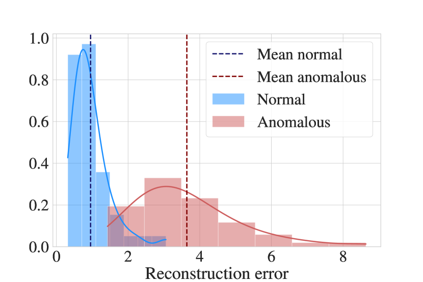
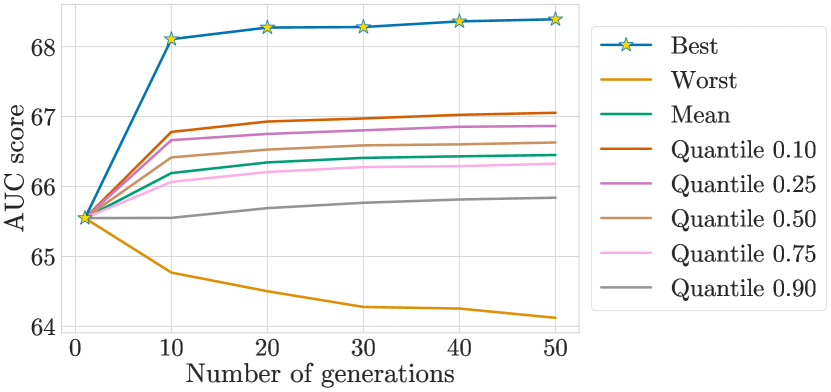
Figure 4: (left) Histograms of the reconstruction errors for 50 synthesized future motions, computed on the HR-UBnormal test set, for the case of conditioning on normal and abnormal past motions. (right) Correlation between the AUC scores and the number of generations, with each curve corresponding to a different aggregation statistic.

5 Discussion

Here, we delve into a detailed discussion about the multimodal future generations (cf Sec. 5.1), the influence of the statistical aggregation of multiple generations and the normal Vs. anomalous conditioning (cf. Sec. 5.2), the effect of different conditioning strategies (cf. Sec. 3.2). Additionally, we discuss forecasting proxy tasks (Sec. 5.4) and analyze MoCoDAD’s performances with the diffusion process applied to the latent space. (Sec. 5.5).

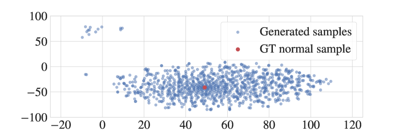
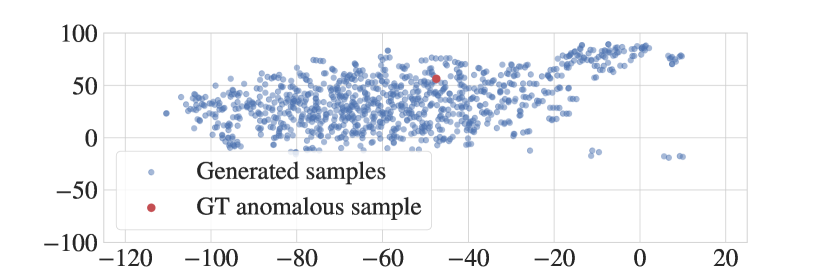
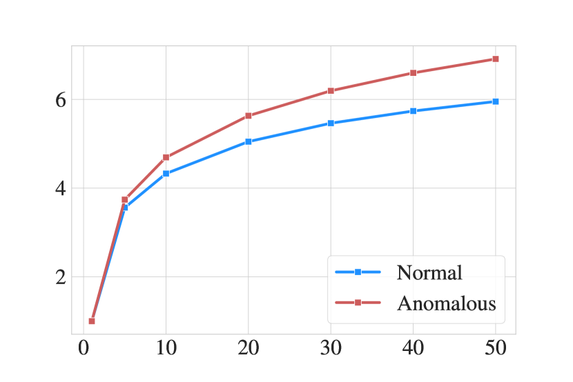
Figure 6: (left) Distribution of 1000 generated future motions, when conditioning on a normal past motion (top) and on an abnormal one (bottom). 2-dimensional projections are estimated via t-SNE [49]. Note how the true future motion (red dot) lies within a main distribution mode in the case of normality, but it lies in a marginal region for abnormality. (right) Plot of the diversity ratio $rF$ [31], measuring the diversity of the generated future motions for normal and anomalous conditioning pasts. Moving along the $x$-axis, with more generated motion, the $rF$ measures grow (MoCoDAD generates multimodal diverse motion) but they remain comparable (generating from normal and abnormal is anyhow multimodal).

5.1 Multimodality

We question whether MoCoDAD can generate diverse multimodal motions and whether conditioning on normal or abnormal motions affects diversity. We provide an example of generated future motions in Fig. 6 (left), where we project the samples in 2D with t-SNE [49] for better visualization. Notice that both sets of generations have similar variance, showing that MoCoDAD produces diverse samples with both normal and abnormal conditioning sequences. Motions stemming from normal conditioning are biased toward the true future since they are mapped around it. Whereas, in the case of abnormal conditioning, the ground truth motion lies on the edge of the predictions’ region, hence being correctly predicted with a lower chance.

We also measure diversity, employing the $rF$ diversity metric from literature [6, 31]. We visualize the $rF$ trend when increasing the number of generations in Fig. 6 (right). If the generated motion had no diversity, e.g., when generating only once, the $rF$ would be equal to 1. Rather, the diversity ratio monotonically increases with the number of generations for both normal and abnormal cases, i.e., the more generated samples, the larger the empirical mode coverage and the diversity. We note that, following intuition, the diversity for abnormal cases grows slightly larger than for normal cases, but the $rF$ measures remain comparable.

5.2 Statistical aggregations of generated motions

We evaluate the anomaly detection performance when varying the number of generations $m$ and the aggregation strategy for the anomaly score $S$ (cf. Sec. 3.1). Fig. 4 (right) shows that the AUC positively correlates with the number of generated future motions for quantiles $Q<0.5$, while the correlation is negative for the mean estimate and $Q>0.5$. Such correlation can be better understood by looking at Fig. 4 (left), which depicts the average reconstruction error probability density function (PDF) for $m=50$: when conditioned on normal past motions, MoCoDAD produces generations which are centered around the true future and, thus, is more likely to yield lower error scores than when generating with abnormal conditioning. The performance saturates for $m>50$.

5.3 Conditioning

Here, we provide the reader with the performances of our method with different encoding approaches of the past (i.e., how the past motion is provided to the model) from which the future is generated (see Table 3).

As illustrated in Sec. 3.2, Input Concatenation concatenates the clean past frames to the corrupted part of each motion sample and feeds it directly to the denoising module. This strategy surpasses recent baselines (cf. Table 1) with AUC scores of $64.96$ and $65.20$ on UBnormal and HR-UBnormal, respectively. We deem this strategy suboptimal since it does not allow the past motion conditioning to be injected at each layer (as with the embedding strategies), and, thus force the network to “remember” this information rather than focusing on the denoising of the future.

The E2E-embedding strategy encodes the motion history in the clean past frames and provides it to the latent layers of the denoising model, but it does not improve performance. We believe this happens because the learned embedding is not supervised, and it may not be representative enough of the original motion.

AE-embedding accounts for the best performances. It couples the encoder $E$ with a symmetric decoder $D$ and trains the whole model with an auxiliary loss $\mathcal{L}_{rec}$ which supervises the reconstruction of the first part of the motion (cf. Sec. 3.2). This past encoding strategy reaches $68.3$ and $68.4$ on UBnormal and HR-UBnormal, outperforming SoA techniques.

Table 3: Ablation study on the different methods for integrating conditioning information into the model.

	HR-UBnormal	UBnormal
Input Concatenation	65.2	65.0
E2E-embedding	64.4	64.2
AE-embedding (MoCoDAD)	68.4	68.3

Table 4: Ablation study on the type of conditioning information to feed into the model to generate the missing frame.

	HR-UBnormal	UBnormal
Random Imputation	65.2	65.1
In-between Imputation	65.7	65.7
Forecasting (MoCoDAD)	68.4	68.3

5.4 Proxy Task

In Table 4 we assess the effectiveness of the forecasting proxy task (cf. Sec. 3.1). To this end, instead of limiting ourselves towards a rigid past-future split of poses, we explore two additional proxy tasks: i.e., in-between and random imputation. For in-between imputation, we corrupt the central $N-k$ poses and reserve the start and end of the sequence to condition the diffusion. For random imputation, we randomly select $N-k$ poses out of the full motion and corrupt them; the rest of the sequence is used for conditioning. Table 4 shows that random imputation is the worst proxy task (AUC of $65.10$ and $65.21$ for UBnormal and HR-UBnormal, respectively). Randomly splitting the sequence into two parts introduces inter-pose temporal gaps. Hence, we believe that this makes the reconstruction of non-contiguous motion more cumbersome. In-between imputation reaches an AUC of $65.65$ and $65.72$, respectively. We think that “stitching” the central motion to its endpoints is an easier task leading both normal and abnormal motions to be equally well reconstructed. Finally, forecasting is the best-performing proxy task with an AUC of $68.3$ and $68.4$ for UBnormal and HR-UBnormal.

5.5 Latent space

Diffusion on latent space has been adopted to improve computational efficiency in various domains [37]. MLD [54] is one of the most recent works in motion forecasting that applies the diffusion process directly in the latent space.

Here, we propose an analysis that assesses the performance of MoCoDAD’s diffusion process in the latent space. Thus, we propose two latent variations of MoCoDAD: MoCoDAD+MLD and Latent-MoCoDAD. For MoCoDAD+MLD we use a VAE to produce a latent representation $Z\in\mathbb{R}^{d}$ of the uncorrupted sequence $X^{k+1:N}$ and we perform the diffusion process on $Z$ with the transformer-based denoising model as described in [54]. For Latent-MoCoDAD we rely on an STS-VAE to learn $Z$ given $X^{k+1:N}$ and use the diffusion process (discussed in Sec. 3.2) on $Z$. For both these variants, we feed the corrupted $Z$ to an MLP with conditioning signal $h+\uptau_{\theta}(t)$ to reverse the diffusion and leave the conditioning component as is in the original MoCoDAD (i.e., encoding of history poses $X^{1:k}$).

Although the described variants can be trained end-to-end, we achieved the best performances by pre-training the autoencoder and training the diffusion module in the learned latent space keeping the autoencoder module frozen. We set the latent space dimension to $d=16$ and the MLP blocks to $(16,8,16)$ interleaved with ReLU activations.

Table 5 illustrates the performances in terms of AUC-ROC of MoCoDAD and its latent variants on UBnormal and HR-UBnormal. Notice that the latent variants underperform w.r.t. the original MoCoDAD. We suspect that diffusion on latent spaces is not effective in skeleton-based VAD due to the lightweight encoding of the skeletons. This adheres with the literature since also MLD [54] shows that applying diffusion in the latent space underperforms w.r.t. the original proposal of the model.

Table 5: AUC-ROC performance of diffusion on latent vs original space.

	HR-UBnormal	UBnormal
MoCoDAD+MLD	58.1	58.1
Latent-MoCoDAD	62.6	62.5
MoCoDAD	68.4	68.3

6 Conclusion

We have presented a novel approach that models and exploits the diversity of normal and abnormal motions. In the former case, the forecast motions are multi-modal and pertinent to the observed portion of the sequence, as the model understands the underlying action. In the case of abnormal, the forecast motions do not show a bias towards the true future as the model does not expect any obvious outcome. Motivated by the improved mode coverage, this work has been the first to take advantage of probabilistic diffusion models for video anomaly detection, including a thorough analysis of the main design choices. MoCoDAD sets a novel SoA among OCC techniques, and it catches up with supervised techniques while not using anomaly training labels.

Supplementary Materials

We supplement the main paper by adding an ablation study on several features of the diffusion process and providing further insights into the conditioning strategies of our method. Additionally, we provide the pseudocode of our proposed framework and describe the implementation details. Finally, we qualitatively illustrate the inference diffusion process, the generated distribution manifolds, and pictograms of input poses with various corrupting types of noise.

Appendix A Diffusion Process

A.1 Background on Diffusion Models

A denoising diffusion probabilistic model (DDPM) [15, 56] exploits two Markov chains: i.e., a forward process and a reverse process. The forward process $q(x_{t}|x_{t-1})$ corrupts the data $x=x_{0}$ gradually adding noise according to a variance schedule $\beta_{t}\in(0,1)$ for $t={1,\ldots,T}$ , transforming any data distribution $q(x_{0})$ into a simple prior (e.g., Gaussian). The forward process can be expressed as

$$q(x_{t}|x_{t-1})=\mathcal{N}(x_{t};\sqrt{1-\beta_{t}}x_{t-1},\beta_{t}\mathbb{I})$$ (6)

To shift the data distribution $q(x_{0})$ toward $q(x_{t}|x_{t-1})$ in one single step, equation 6 can be reformulated as

$$q(x_{t}|x_{0})=\mathcal{N}(x_{t};\sqrt{\bar{\alpha_{t}}}x_{0},(1-\bar{\alpha_{t}})\mathbb{I})$$ (7)

with $\alpha_{t}:=1-\beta_{t}$ and $\bar{\alpha_{t}}:=\prod^{t}_{s=1}\alpha_{s}$.

The reverse process leans to roll back this degradation. More formally, the reverse process can be formulated as

$$p_{\theta}(x_{t-1}|x_{t})=\mathcal{N}\big{(}x_{t-1};\mu_{\theta}(x_{t},t),\beta_{t}\mathbb{I}\big{)}$$ (8)

where $\mu_{\theta}(x_{t},t)$ is a deep neural network that estimates the forward process posterior mean. [15] has shown that one obtains high-quality samples when optimizing the objective

$$\mathcal{L}_{simple}=\underset{t,x_{0},\varepsilon}{\mathbb{E}}\bigg{[}\big{|}\big{|}\varepsilon-\varepsilon_{\theta}\big{(}\sqrt{\bar{\alpha_{t}}}x_{0}+\sqrt{1-\bar{\alpha_{t}}}\;\varepsilon,t\big{)}\big{|}\big{|}^{2}_{2}\bigg{]}$$ (9)

where $\varepsilon\sim\mathcal{N}(0,\mathbb{I})$ is the noise used to corrupt the sample $x_{0}$, and $\varepsilon_{\theta}$ is a neural network trained to predict $\varepsilon$.

During inference, the sampling algorithm of [15] is used to iteratively denoise random Gaussian noise $x_{T}\sim\mathcal{N}(0,\mathbb{I})$, to generate a sample from the learned distribution. [35, 37] have shown that one may condition DDPMs on a signal $h$ by feeding it to the neural network $\epsilon_{\theta}$.

A.2 Diffusive steps

Sec. 3 in the main paper delineates a gradual corruption technique that employs a displacement map in accordance with a variance scheduler $\beta_{t}\in(0,1)$ to corrupt the input. The degree of displacement applied is determined by $\beta_{t}$ which follows a schedule based on the parameter $t$.

To further investigate the relationship between the diffusive steps and performance, we evaluate the impact of varying $t$ on the performance of MoCoDAD. As shown in Table 6, we consider five different steps $t\in\{2,5,10,25,50\}$. Our results demonstrate that optimal performances occur with 10 diffusive steps while deteriorating for any higher or lower value.

Note that this optimal $T$ value is significantly smaller than those used in other diffusion approaches [15, 30, 34, 47] which require a large number of steps to turn a noisy sample $x_{T}\in\mathcal{N}(0,I)$ into a semantically significant one.

On the contrary, our model’s strong inductive bias towards poses, together with its ability to leverage the invariant relationships and dependencies between intra-pose joints allows it to transform a set of random joint positions $x_{T}\in\mathcal{N}(0,I)$ into a pose-like structure in just one step, as illustrated in Figure 9. Furthermore, we highlight that a small $T$ can push the model to improve the quality of normal poses while failing to refine abnormal ones. Thereby, employing a $T=10$ we allow MoCoDAD to foster this trade-off and obtain optimal performances.

Additionally, to highlight the effectiveness of the iterative diffusion process we evaluate the model with $T=2$, that is, the case where the model only receives either clean or completely corrupted input poses: this means that during inference the model performs the denoising non-iteratively, e.g. in one single step. The resulting model underperforms w.r.t. MoCoDAD, confirming the importance of a multi-step diffusion process.

Table 6: AUC-ROC performance variation of MoCoDAD on the number of employed diffusive steps $t$ of the variance scheduler $\beta_{t}$.

Diffusive steps	HR-UBnormal	UBnormal
2	65.0	64.7
5	66.3	65.9
10	68.4	68.3
25	64.70	64.6
50	64.4	64.4

Appendix B Weaker forms of conditioning

In Table 7, we complement the experiments in Sec. 5.3 of the main paper with an additional discussion on the forms of conditioning. Following the approach proposed by [52], we investigate two aspects: applying an alternative sampling strategy and using a different corruption function instead of the Gaussian one. We also evaluate the effectiveness of MoCoDAD in the absence of conditioning past motion frames.

Regarding the alternative sampling strategy, we train our diffusion model to denoise a corrupted sample $x_{t}$, where $t\in\{1,\ldots,T\}$ and $T=10$, while, during inference, we perform sampling starting from partially corrupted samples $x_{\gamma}$ where $\gamma<T$. The partially corrupted signal acts as a weaker form of conditioning, i.e., generating by denoising the signal. Hence, the reverse diffusion process does not need to be conditioned on past frames.

Table 7: Impact of different noise distributions and sampling strategies on performance in terms of AUC-ROC. MoCo refers to Motion Condition; $T$ represents the diffusion step at which samples are completely corrupted; $\gamma$ represents the step up to which samples are corrupted during inference. The last row illustrates our proposed method, MoCoDAD.

$\gamma/T$	Corruption	MoCo	HR-UBnormal	UBnormal
3/10	Simplex	$\times$	53.0	52.0
3/10	Gaussian	$\times$	57.4	57.3
10/10	Gaussian	$\times$	55.0	54.1
10/10	Gaussian	✓	68.4	68.3

The first column of Table 7 refers to the timesteps used at inference time ($\gamma$) and the ones used at training ($T$). Following [52], we set $\gamma$ to be equal to a third of $T$. When the denoising process begins with a partially corrupted image (first and second rows), the results degrade to 52 and 57.35, respectively. We explain this since, even in the absence of prior motion, the starting point of the denoising process is more similar to the target signal, reducing the reconstruction error for both normal and abnormal samples.

We investigate this intuition by comparing two different noise distributions to randomly corrupt the poses, namely Gaussian and Simplex noise [32]. Fig. 8 compares the joint displacement at $t\in\{3,6,9\}$ for both these noise distributions. We see that Gaussian corrupts the input motion more since every joint is translated with a random intensity, whereas, Simplex acts as a weaker perturber maintaining a significant amount of information from the original motion. This reflects in performance. Table 7 shows that adding Simplex noise is not effective with motion sequences, deteriorating the overall performances to 52 (see row 1).

Next, we consider generating future motions without conditioning on the past. In the absence of conditioning past frames, the model is expected to provide samples from the learned training normal distribution. Therefore, it still makes sense to consider this approach for anomaly detection by comparing similarities of generated and true futures. In fact, the generated future frames will be normal, more similar to normal true futures, and less similar to abnormal true futures. Note, however, that missing to condition on the past will result in general futures unrelated to the specific past, just normal. The results in Table 7 support this observation, i.e. the performance reduces to 54.11, close to the chance level (50%).

To sum up, neither the Gaussian nor the Simplex noise provide comparable performance with MoCoDAD  confirming the need for a conditioning signal to govern the diffusion process.

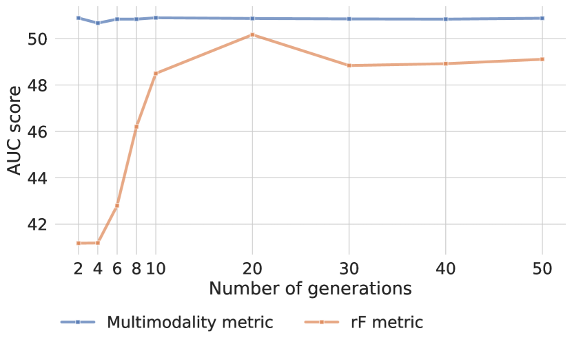
Figure 7: Anomaly detection performance trend when assuming a diversity metric as the anomaly score. It is worth noting that the $rF$ metric yields results that are below the chance level.

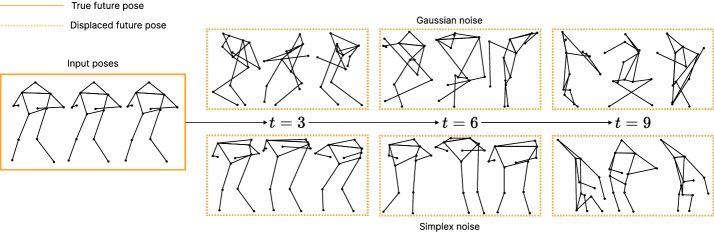
Figure 8: Comparison of Gaussian (up) vs Simplex (down) noises applied to a sequence of future poses.

Appendix C MoCoDAD Algorithms

In this section, we outline the algorithms designed for both the training and inference phases of our proposed model (cf. Sec. 3.2 of the main paper). In algorithms 1 and 2, we employ the following notation: $\bar{\cdot}$ denotes the objects that are encoded in a latent space, whereas $\hat{\cdot}$ signifies the predictions of our model.

Train. In Alg. 1 we describe the training process for a single sequence of poses $X^{1:N}$. The algorithm only requires the input sequence, the current timestep $t$, the parameters $\lambda_{1}$ and $\lambda_{2}$ governing the importance of the two losses, and the MoCoDAD modules introduced in Sec. 3.3 of the main paper.

Inference. Alg. 2 depicts how our proposed method assigns the anomaly score to each frame of a video. For readability purposes, we only examine the case of a single window $\mathcal{W}$, which encompasses the frames $f_{1},f_{2},...,f_{N}$. We adopt a sliding window procedure to analyze each video so that Alg. 2 can be further extended to assess all the frames of a video. First, we extract the poses of all the subjects whose motion lies in all the frames of $\mathcal{W}$, resulting in the set $\mathcal{A}$. Then, starting from random noise $\varepsilon$, we iteratively leverage MoCoDAD to draw $m$ possible futures in $T$ steps (see Fig. 9), which we subsequently compare with the GT future to distill $m$ scores for each sample $X_{a}^{1:N}$ (collected in the set $\mathcal{G}$). As discussed in Sec. 3.2 of the main paper, we then aggregate these scores in a single value ($\mathcal{H}_{a}$, which we interpret as the anomaly score of the subject $a$ for the frames in $\mathcal{W}$). Note that, when considering multiple overlapping time windows

$$\mathcal{W}^{(1)}[f_{1}:f_{N}],\mathcal{W}^{(2)}[f_{2}:f_{N+1}],...,\mathcal{W}^{(N)}[f_{N}:f_{2N-1}],$$

$\mathcal{H}_{a}$ is computed as $\max(\mathcal{H}_{a}^{(1)},...,\mathcal{H}_{a}^{(N)})$. Finally, we repeat this process for each actor appearing in the scene and accumulate these local scores in the set $\mathcal{S}$. We compute the mean, the maximum, and the minimum of $\mathcal{S}$ and attribute to each frame $f_{1},...,f_{N}$ the anomaly score (AS) defined as follows:

$$\mathrm{AS}[f_{1}:f_{N}]=\mathrm{mean}(\mathcal{S})+\log\frac{1+\max(\mathcal{S})}{1+\min(\mathcal{S})}.$$ (10)

While the $\mathrm{mean}(\mathcal{S})$ summarizes the distribution of the maximum errors of all actors within each frame, the second term takes into account the width of the errors range, as it is mathematically equivalent to:

$$\log\left(1+\max\left(\mathcal{S}\right)\right)-\log\left(1+\min\left({\mathcal{S}}\right)\right).$$ (11)

This increases the anomaly score for spread distributions, which likely correspond to anomalous frames; the logarithm function prevents this term from dominating the final anomaly score.

Algorithm 1 MoCoDAD Train

0:  $X^{1:N},t,\lambda_{1},\lambda_{2}$

  // Divide past from future poses

  $\mathcal{P},\ \mathcal{F}=X^{1:k},\ X^{k+1:N}$

  // Condition Encoding

  $\mathcal{\overline{P}}=\text{E}(\mathcal{P})\ ;\ \ \mathcal{\hat{P}}=\text{D}(\mathcal{\overline{P}})$

  $\tau=\uptau_{\theta}(t)$

  // Forward Diffusion

  $\mathcal{F}_{t}=q(\mathcal{F},t)$

  // Engender futures

  $\mathcal{\hat{F}}=\text{MoCoDAD}(\mathcal{F}_{t};\tau,\mathcal{\overline{P}})$

  // Loss

  $Loss=\lambda_{1}\mathcal{L}_{smooth}(\mathcal{\hat{F}},\mathcal{F})+\lambda_{2}\mathcal{L}_{rec}(\mathcal{\hat{P}},\mathcal{P})$

Algorithm 2 MoCoDAD Inference

0:  $\mathcal{W}=\{f_{1},...,f_{N}\}$, $\mathcal{A}=\{\text{actors}\;|\;\text{actors}\in f_{i}\ \forall f_{i}\in\mathcal{W}\}$, $m,\ T,\ \mathcal{G}=\varnothing,\ \mathcal{S}=\varnothing$

  for all $a\in\mathcal{A}$ do

     // Extract and embed past poses

     $\mathcal{P},\ \mathcal{F}=X^{1:k}_{a},\ X^{k+1:N}_{a}$

     $\mathcal{\overline{P}}=\text{E}(\mathcal{P})$

     // Sample random noise

     $\varepsilon\sim\mathcal{N}(0,\textbf{I})$

     // Engender futures

     for $j\leftarrow 0$ to $m$ do

        $\mathcal{F}_{j,T}\leftarrow\varepsilon$

        // Reverse diffusion

        for $t\leftarrow T$ to $1$ do

           $\tau=\uptau_{\theta}(t)$

           $\mathcal{\hat{F}}_{j}=\text{MoCoDAD}(\mathcal{F}_{j,t};\tau,\mathcal{\overline{P}})$

           // Forward Diffusion

           $\mathcal{F}_{j,t-1}=q(\mathcal{\hat{F}}_{j},t-1)$

        end for

        // Get generation anomaly score

        $\text{SCORE}_{j}=\mathcal{L}_{smooth}(\mathcal{\hat{F}}_{j},\mathcal{F})$

        $\mathcal{G}\leftarrow\mathcal{G}\cup\{\text{SCORE}_{j}\}$

     end for

     // Aggregate generations

     $\mathcal{H}_{a}=\text{AGGREGATE}(\mathcal{G})$

     $\mathcal{S}\leftarrow\mathcal{S}\cup\{\mathcal{H}_{a}\}$

  end for

  // Impute frames’ Anomaly Score

  $\text{AS}[f_{1}:f_{N}]=\mathrm{mean}(\mathcal{S})+\log\frac{1+\max(\mathcal{S})}{1+\min(\mathcal{S})}$

Appendix D Further notes on multimodality

We complement Sec. 5.2 of the main paper by showing that multimodality cannot be exploited for separating normal and abnormal classes, since both have a similar degree of diversity (cf. Sec. 3.2).

As for the diversity metrics, we employ the $rF$ metric [6, 31] (see Sec. 3.2) and the Multimodality metric proposed in [13].

Multimodality measures the variance among generated motions given the same conditioning sequence. For each sample $s$, let $\mathcal{S}$ be the set of all generated motions; then, two subsets $\mathcal{A}(s)=\{\mathbf{a}_{1},...,\mathbf{a}_{S_{m}}\}$ and $\mathcal{B}(s)=\{\mathbf{b}_{1},...,\mathbf{b}_{S_{m}}\}$ are sampled from $\mathcal{S}$. Finally, Multimodality is given by:

$$\mathrm{Multimodality}(s)=\frac{1}{S_{m}}\underset{i=1}{\overset{S_{m}}{\sum}}\|\mathbf{a}_{i}-\mathbf{b}_{i}\|_{2}$$ (12)

Comparing with Fig. 4 (right) of the main paper, the plot in Fig. 7 clearly shows that the anomaly detection performance dramatically drops when assuming a diversity metric as the anomaly score, nearly to random chance. It is worth noting that the performance drops even below random chance when evaluating with $rF$ for a number of generations less than 10.

Appendix E Implementation details

As in [9, 27, 28], we adopt a sliding window procedure for dividing each agent’s motion history. We use a window size of 6 frames for all the experiments, of which the first 3 are taken for the condition and the rest for the diffusion process. We adopt similar setups for the imputation proxy tasks (see Sec. 5.4). We set $\lambda_{1}=\lambda_{2}=1$. We train the network end-to-end with the Adam optimizer [20] and a learning rate of $1e^{-4}$ with exponential decay for 36 epochs. The diffusion process uses $\beta_{1}=1e^{-4}$ and $\beta_{T}=2e^{-2}$, $T=10$ and the cosine variance scheduler from [30].

Our U-Net-GCN downscales the joints from $17$ to $10$ and expands the channels from $2$ to $(32,32,64,64,128,64)$. The conditioning encoder has a channel sequence of $(32,16,32)$, with a bottleneck of $32$ and a latent projector of $16$. We encode the timestep with the positional encoding as defined in [50]. Our training took approximately 7 hours on an Nvidia Quadro P6000 GPU.

Appendix F Results on the UBnormal Validation set

Table 8: Comparison of MoCoDAD against SoA in terms of AUC-ROC on the validation set of UBnormal. OCC skeleton-based techniques ($*$) are directly comparable to MoCoDAD. Supervised (${\dagger}$) and weakly supervised (${\ddagger}$) methods are also reported, grayed-out since they leverage extra annotations.

	UBnormal
Sultani et al. [45] ${\dagger}$	51.8
AED-SSMTL [10] ${\dagger}$	68.2
TimeSformer [4] ${\dagger}$	86.1
AED-SSMTL [10] ${\ddagger}$	58.5
MPED-RNN [28] $*$	61.2
GEPC [27] $*$	47.0
COSKAD [9] $*$	76.4
MoCoDAD $*$	77.6

Validation performance is not reported in the main paper, as the validation set is used for hyperparameter fine-tuning. For completeness purposes, as done in [1], we report MoCoDAD’s performances vs SoA on the validation set of UBnormal.

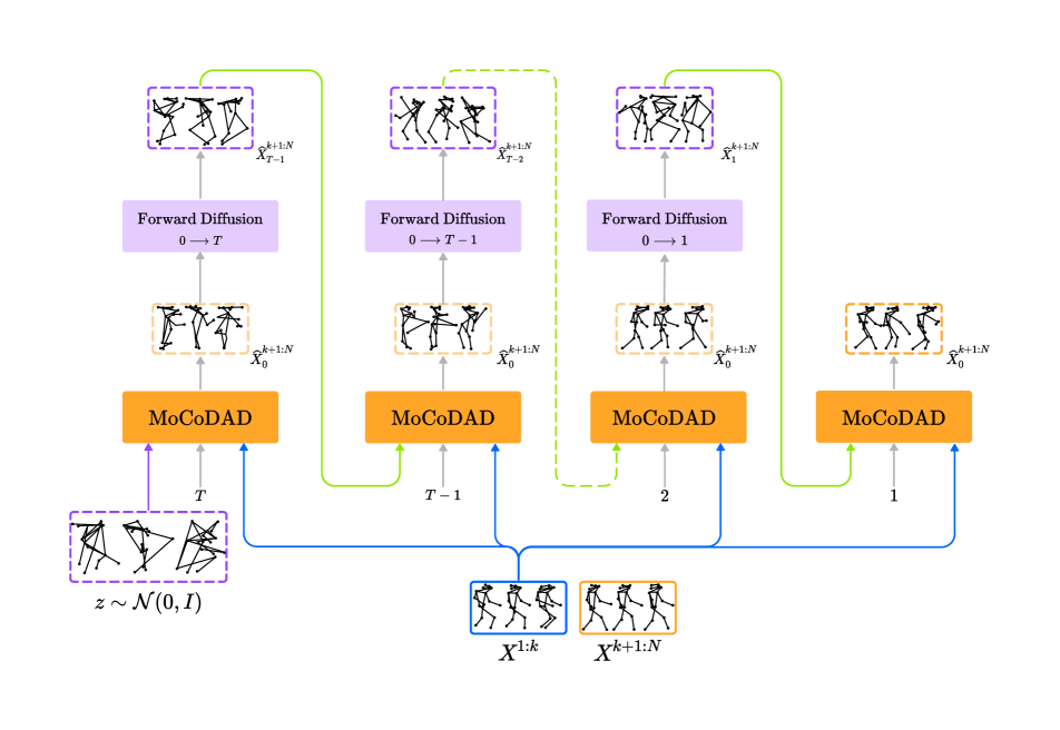
Figure 9: The iterative sampling process of our proposed method (cf. Sec. 3.2 in the main paper). At each step, MoCoDAD generates a prediction (light orange dashed boxes) employing a pose (purple dashed boxes) displaced proportionally to the current timestep $t$ (when $t=T$ we just sample from random noise), together with a prior motion encoding $X^{1:k}$ and the current timestep $t$. The current prediction is then fed to the Forward Diffusion module, which adds a displacement map to it, anew corrupting the pose proportionally to a smaller timestep. This process is iteratively repeated from $T$ to $1$, continuously refining the prediction which is then compared with the actual future (orange box).

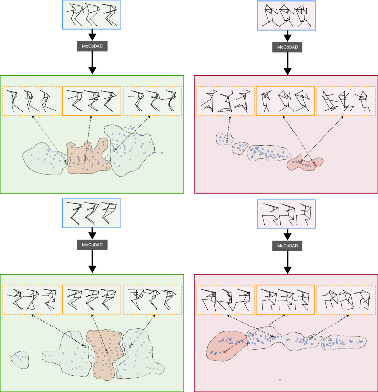
Figure 10: MoCoDAD detects anomalies by synthesizing and statistically aggregating multimodal future motions, conditioned on past frames. Red (right) and green (left) represent examples of anomaly and normality. At the bottom, 100 futures (2d mapped via t-SNE) are generated (dashed-orange rectangles) via a diffusion probabilistic model, conditioned on the past frames (blue-outlined rectangles). Within the distribution modes (highlighted contours), the red dots are the actual true futures corresponding to the sequence of future poses (orange-outlined rectangles). In the case of normality, the true future lies within a main distribution mode, and the generated predictions are pertinent. In the case of abnormality, the true future lies in the tail of the distribution modes, which yields poorer predictions, highlighting anomalies.

Table 8 shows that the validation set results are in line with those on the test sets reported in Table 1 of the main paper. Notice that MoCoDAD outperforms all the other OCC approaches reaching an AUC of $77.6$. Additionally, considering (weakly) supervised approaches that require labeled data (anomalies included), MoCoDAD is only second to TimeSformer [4].

Appendix G Generating motion sequences

This section visually illustrates how a sample is generated using the reverse procedure (Fig. 9). This supplements the discussion presented in Sec. 3 (main paper), providing a visual explanation of Eq. 7. MoCoDAD generates motion sequences depending on a particular conditioning signal, as explained in Section 3 of the main paper. This process is shown graphically in Fig. 9. Random noise $x_{T}$ in the dimensions corresponding to the desired motion is initially sampled. The process then proceeds iteratively from step $T$ to $1$. MoCoDAD predicts a clean sample $x_{0}$ at each step $t$, then diffuses back to the previous $X_{t-1}$.

Appendix H Qualitative results

Fig. 10 reveals that the generations produced with normal conditioning are biased towards the true future. The figure illustrates the t-SNE [49] 2D-embeddings of the generated future frames (orange rectangles), conditioned on the past (blue rectangles). Here, we present two groups of illustrations based on normal (green) and abnormal (red) past, respectively. When the conditioning is normal, the generations (dashed-orange rectangles) are nearby the true motion which lies at the center of the distribution. However, when the past is anomalous, the true future is significantly distant from the center of the distribution produced. Since the diffusion process can generate multiple plausible futures - contoured shapes in the figure - this enforces our assertion that MoCoDAD is multimodal in both normal and anomalous contexts. In the former case, it is capable of generating samples that are much more pertinent to the actual future; while, in the latter, the generated samples yield poorer predictions, highlighting anomalies (e.g., the first generation in the upper-right corner, and the second generation in the lower-right corner).

References

- [1] Andra Acsintoae, Andrei Florescu, Mariana-Iuliana Georgescu, Tudor Mare, Paul Sumedrea, Radu Tudor Ionescu, Fahad Shahbaz Khan, and Mubarak Shah. Ubnormal: New benchmark for supervised open-set video anomaly detection. In Proceedings of the IEEE/CVF Conference on Computer Vision and Pattern Recognition, pages 20143–20153, 2022.
- [2] Emre Aksan, Manuel Kaufmann, Peng Cao, and Otmar Hilliges. A spatio-temporal transformer for 3d human motion prediction. In 2021 International Conference on 3D Vision (3DV), pages 565–574. IEEE, 2021.
- [3] Antonio Barbalau, Radu Tudor Ionescu, Mariana-Iuliana Georgescu, Jacob Dueholm, Bharathkumar Ramachandra, Kamal Nasrollahi, Fahad Shahbaz Khan, Thomas B. Moeslund, and Mubarak Shah. Ssmtl++: Revisiting self-supervised multi-task learning for video anomaly detection. Computer Vision and Image Understanding, 229:103656, 2023.
- [4] Gedas Bertasius, Heng Wang, and Lorenzo Torresani. Is space-time attention all you need for video understanding? In Proceedings of the International Conference on Machine Learning (ICML), page 4, 2021.
- [5] Simone Calderara, Uri Heinemann, Andrea Prati, Rita Cucchiara, and Naftali Tishby. Detecting anomalies in people’s trajectories using spectral graph analysis. Computer Vision and Image Understanding, 115(8):1099–1111, 2011.
- [6] Laura Calem, Hedi Ben-Younes, Patrick Pérez, and Nicolas Thome. Diverse probabilistic trajectory forecasting with admissibility constraints. In 2022 26th International Conference on Pattern Recognition (ICPR), pages 3478–3484, 2022.
- [7] Yong Shean Chong and Yong Haur Tay. Abnormal event detection in videos using spatiotemporal autoencoder. In Advances in Neural Networks-ISNN 2017: 14th International Symposium, ISNN 2017, Sapporo, Hakodate, and Muroran, Hokkaido, Japan, June 21–26, 2017, Proceedings, Part II 14, pages 189–196. Springer, 2017.
- [8] Prafulla Dhariwal and Alexander Nichol. Diffusion models beat gans on image synthesis. Advances in Neural Information Processing Systems, 34:8780–8794, 2021.
- [9] Alessandro Flaborea, Guido D’Amely, Stefano D’Arrigo, Marco Aurelio Sterpa, Alessio Sampieri, and Fabio Galasso. Contracting skeletal kinematics for human-related video anomaly detection, 2023.
- [10] Mariana-Iuliana Georgescu, Antonio Barbalau, Radu Tudor Ionescu, Fahad Shahbaz Khan, Marius Popescu, and Mubarak Shah. Anomaly detection in video via self-supervised and multi-task learning. In Proceedings of the IEEE/CVF Conference on Computer Vision and Pattern Recognition (CVPR), pages 12742–12752, June 2021.
- [11] Ross Girshick. Fast r-cnn. In Proceedings of the IEEE international conference on computer vision, pages 1440–1448, 2015.
- [12] Dong Gong, Lingqiao Liu, Vuong Le, Budhaditya Saha, Moussa Reda Mansour, Svetha Venkatesh, and Anton van den Hengel. Memorizing normality to detect anomaly: Memory-augmented deep autoencoder for unsupervised anomaly detection. In Proceedings of the IEEE/CVF International Conference on Computer Vision, pages 1705–1714, 2019.
- [13] Chuan Guo, Xinxin Zuo, Sen Wang, Shihao Zou, Qingyao Sun, Annan Deng, Minglun Gong, and Li Cheng. Action2motion: Conditioned generation of 3d human motions. In Proceedings of the 28th ACM International Conference on Multimedia, pages 2021–2029, 2020.
- [14] Mahmudul Hasan, Jonghyun Choi, Jan Neumann, Amit K Roy-Chowdhury, and Larry S Davis. Learning temporal regularity in video sequences. In Proceedings of the IEEE conference on computer vision and pattern recognition, pages 733–742, 2016.
- [15] Jonathan Ho, Ajay Jain, and Pieter Abbeel. Denoising diffusion probabilistic models. In Proceedings of the 34th International Conference on Neural Information Processing Systems, NIPS’20, Red Hook, NY, USA, 2020. Curran Associates Inc.
- [16] Yashswi Jain, Ashvini Kumar Sharma, Rajbabu Velmurugan, and Biplab Banerjee. Posecvae: Anomalous human activity detection. In 2020 25th International Conference on Pattern Recognition (ICPR), pages 2927–2934. IEEE, 2021.
- [17] Fan Jiang, Junsong Yuan, Sotirios A Tsaftaris, and Aggelos K Katsaggelos. Anomalous video event detection using spatiotemporal context. Computer Vision and Image Understanding, 115(3):323–333, 2011.
- [18] Asiegbu Miracle Kanu-Asiegbu, Ram Vasudevan, and Xiaoxiao Du. Bipoco: Bi-directional trajectory prediction with pose constraints for pedestrian anomaly detection. arXiv preprint arXiv:2207.02281, 2022.
- [19] Shehroz S Khan and Michael G Madden. One-class classification: taxonomy of study and review of techniques. The Knowledge Engineering Review, 29(3):345–374, 2014.
- [20] Diederik P. Kingma and Jimmy Ba. Adam: A method for stochastic optimization. CoRR, abs/1412.6980, 2015.
- [21] Ce Li, Zhenjun Han, Qixiang Ye, and Jianbin Jiao. Visual abnormal behavior detection based on trajectory sparse reconstruction analysis. Neurocomputing, 119:94–100, 2013.
- [22] Nanjun Li, Faliang Chang, and Chunsheng Liu. Human-related anomalous event detection via spatial-temporal graph convolutional autoencoder with embedded long short-term memory network. Neurocomputing, 490:482–494, 2022.
- [23] Wen Liu, Weixin Luo, Dongze Lian, and Shenghua Gao. Future frame prediction for anomaly detection–a new baseline. In Proceedings of the IEEE conference on computer vision and pattern recognition, pages 6536–6545, 2018.
- [24] Cewu Lu, Jianping Shi, and Jiaya Jia. Abnormal event detection at 150 fps in matlab. In Proceedings of the IEEE international conference on computer vision, pages 2720–2727, 2013.
- [25] Weixin Luo, Wen Liu, and Shenghua Gao. A revisit of sparse coding based anomaly detection in stacked rnn framework. In Proceedings of the IEEE international conference on computer vision, pages 341–349, 2017.
- [26] Weixin Luo, Wen Liu, and Shenghua Gao. Normal graph: Spatial temporal graph convolutional networks based prediction network for skeleton based video anomaly detection. Neurocomputing, 444:332–337, 2021.
- [27] Amir Markovitz, Gilad Sharir, Itamar Friedman, Lihi Zelnik-Manor, and Shai Avidan. Graph embedded pose clustering for anomaly detection. In Proceedings of the IEEE/CVF Conference on Computer Vision and Pattern Recognition, pages 10539–10547, 2020.
- [28] Romero Morais, Vuong Le, Truyen Tran, Budhaditya Saha, Moussa Mansour, and Svetha Venkatesh. Learning regularity in skeleton trajectories for anomaly detection in videos. In Proceedings of the IEEE/CVF conference on computer vision and pattern recognition, pages 11996–12004, 2019.
- [29] Duc Tam Nguyen, Zhongyu Lou, Michael Klar, and Thomas Brox. Anomaly detection with multiple-hypotheses predictions. In International Conference on Machine Learning, pages 4800–4809. PMLR, 2019.
- [30] Alexander Quinn Nichol and Prafulla Dhariwal. Improved denoising diffusion probabilistic models. In International Conference on Machine Learning, pages 8162–8171. PMLR, 2021.
- [31] Seong Hyeon Park, Gyubok Lee, Jimin Seo, Manoj Bhat, Minseok Kang, Jonathan Francis, Ashwin Jadhav, Paul Pu Liang, and Louis-Philippe Morency. Diverse and admissible trajectory forecasting through multimodal context understanding. In Computer Vision–ECCV 2020: 16th European Conference, Glasgow, UK, August 23–28, 2020, Proceedings, Part XI 16, pages 282–298. Springer, 2020.
- [32] Ken Perlin. Improving noise. In Proceedings of the 29th annual conference on Computer graphics and interactive techniques, pages 681–682, 2002.
- [33] Mathis Petrovich, Michael J Black, and Gül Varol. Action-conditioned 3d human motion synthesis with transformer vae. In Proceedings of the IEEE/CVF International Conference on Computer Vision, pages 10985–10995, 2021.
- [34] Aditya Ramesh, Prafulla Dhariwal, Alex Nichol, Casey Chu, and Mark Chen. Hierarchical text-conditional image generation with CLIP latents. CoRR, abs/2204.06125, 2022.
- [35] Aditya Ramesh, Mikhail Pavlov, Gabriel Goh, Scott Gray, Chelsea Voss, Alec Radford, Mark Chen, and Ilya Sutskever. Zero-shot text-to-image generation. In Marina Meila and Tong Zhang, editors, Proceedings of the 38th International Conference on Machine Learning, volume 139 of Proceedings of Machine Learning Research, pages 8821–8831. PMLR, 18–24 Jul 2021.
- [36] Royston Rodrigues, Neha Bhargava, Rajbabu Velmurugan, and Subhasis Chaudhuri. Multi-timescale trajectory prediction for abnormal human activity detection. In The IEEE Winter Conference on Applications of Computer Vision (WACV), March 2020.
- [37] Robin Rombach, Andreas Blattmann, Dominik Lorenz, Patrick Esser, and Björn Ommer. High-resolution image synthesis with latent diffusion models. In 2022 IEEE/CVF Conference on Computer Vision and Pattern Recognition (CVPR), pages 10674–10685, 2022.
- [38] Lukas Ruff, Robert Vandermeulen, Nico Goernitz, Lucas Deecke, Shoaib Ahmed Siddiqui, Alexander Binder, Emmanuel Müller, and Marius Kloft. Deep one-class classification. In International conference on machine learning, pages 4393–4402. PMLR, 2018.
- [39] Saeed Saadatnejad, Ali Rasekh, Mohammadreza Mofayezi, Yasamin Medghalchi, Sara Rajabzadeh, Taylor Mordan, and Alexandre Alahi. A generic diffusion-based approach for 3d human pose prediction in the wild. In NeurIPS 2022 Workshop on Score-Based Methods, 2022.
- [40] Mohammad Sabokrou, Mohsen Fayyaz, Mahmood Fathy, and Reinhard Klette. Deep-cascade: Cascading 3d deep neural networks for fast anomaly detection and localization in crowded scenes. IEEE Transactions on Image Processing, 26(4):1992–2004, 2017.
- [41] Alessio Sampieri, Guido Maria D’Amely di Melendugno, Andrea Avogaro, Federico Cunico, Francesco Setti, Geri Skenderi, Marco Cristani, and Fabio Galasso. Pose forecasting in industrial human-robot collaboration. In Computer Vision – ECCV 2022, pages 51–69, Cham, 2022. Springer Nature Switzerland.
- [42] Bernhard Schölkopf, John C Platt, John Shawe-Taylor, Alex J Smola, and Robert C Williamson. Estimating the support of a high-dimensional distribution. Neural computation, 13(7):1443–1471, 2001.
- [43] Theodoros Sofianos, Alessio Sampieri, Luca Franco, and Fabio Galasso. Space-time-separable graph convolutional network for pose forecasting. In Proceedings of the IEEE/CVF International Conference on Computer Vision, pages 11209–11218, 2021.
- [44] Jascha Sohl-Dickstein, Eric Weiss, Niru Maheswaranathan, and Surya Ganguli. Deep unsupervised learning using nonequilibrium thermodynamics. In Francis Bach and David Blei, editors, Proceedings of the 32nd International Conference on Machine Learning, volume 37 of Proceedings of Machine Learning Research, pages 2256–2265, Lille, France, 07–09 Jul 2015. PMLR.
- [45] Waqas Sultani, Chen Chen, and Mubarak Shah. Real-world anomaly detection in surveillance videos. In Proceedings of the IEEE conference on computer vision and pattern recognition, pages 6479–6488, 2018.
- [46] David MJ Tax and Robert PW Duin. Support vector data description. Machine learning, 54:45–66, 2004.
- [47] Guy Tevet, Sigal Raab, Brian Gordon, Yoni Shafir, Daniel Cohen-or, and Amit Haim Bermano. Human motion diffusion model. In The 11th International Conference on Learning Representations, 2023.
- [48] Hoang Thanh-Tung and Truyen Tran. Catastrophic forgetting and mode collapse in gans. In 2020 international joint conference on neural networks (ijcnn), pages 1–10. IEEE, 2020.
- [49] Laurens Van der Maaten and Geoffrey Hinton. Visualizing data using t-sne. Journal of machine learning research, 9(11), 2008.
- [50] Ashish Vaswani, Noam Shazeer, Niki Parmar, Jakob Uszkoreit, Llion Jones, Aidan N Gomez, Ł ukasz Kaiser, and Illia Polosukhin. Attention is all you need. In I. Guyon, U. Von Luxburg, S. Bengio, H. Wallach, R. Fergus, S. Vishwanathan, and R. Garnett, editors, Advances in Neural Information Processing Systems, volume 30. Curran Associates, Inc., 2017.
- [51] Zhiwei Wang, Zhengzhang Chen, Jingchao Ni, Hui Liu, Haifeng Chen, and Jiliang Tang. Multi-scale one-class recurrent neural networks for discrete event sequence anomaly detection. In Proceedings of the 27th ACM SIGKDD conference on knowledge discovery & data mining, pages 3726–3734, 2021.
- [52] Julian Wyatt, Adam Leach, Sebastian M. Schmon, and Chris G. Willcocks. Anoddpm: Anomaly detection with denoising diffusion probabilistic models using simplex noise. In Proceedings of the IEEE/CVF Conference on Computer Vision and Pattern Recognition (CVPR) Workshops, pages 650–656, June 2022.
- [53] Zhisheng Xiao, Karsten Kreis, and Arash Vahdat. Tackling the generative learning trilemma with denoising diffusion GANs. In International Conference on Learning Representations (ICLR), 2022.
- [54] Chen Xin, Biao Jiang, Wen Liu, Zilong Huang, Bin Fu, Tao Chen, Jingyi Yu, and Gang Yu. Executing your commands via motion diffusion in latent space. In Proceedings of the IEEE/CVF Conference on Computer Vision and Pattern Recognition (CVPR), June 2023.
- [55] Sijie Yan, Yuanjun Xiong, and Dahua Lin. Spatial temporal graph convolutional networks for skeleton-based action recognition. In Proceedings of the AAAI conference on artificial intelligence, volume 32, 2018.
- [56] Ling Yang, Zhilong Zhang, Yang Song, Shenda Hong, Runsheng Xu, Yue Zhao, Yingxia Shao, Wentao Zhang, Ming-Hsuan Yang, and Bin Cui. Diffusion models: A comprehensive survey of methods and applications. CoRR, abs/2209.00796, 2022.
- [57] Ye Yuan and Kris Kitani. Dlow: Diversifying latent flows for diverse human motion prediction. In Proceedings of the European Conference on Computer Vision (ECCV), 2020.
- [58] Yiru Zhao, Bing Deng, Chen Shen, Yao Liu, Hongtao Lu, and Xian-Sheng Hua. Spatio-temporal autoencoder for video anomaly detection. In Proceedings of the 25th ACM international conference on Multimedia, pages 1933–1941, 2017.
- [59] Linqi Zhou, Yilun Du, and Jiajun Wu. 3d shape generation and completion through point-voxel diffusion. In Proceedings of the IEEE/CVF International Conference on Computer Vision (ICCV), pages 5826–5835, October 2021.