\Qcircuit@C=0.3em@R=.4em\Qcircuit@𝐶0.3𝑒𝑚@𝑅.4𝑒𝑚\displaystyle\Qcircuit@C=0.3em@R=.4em layer $l$
$\displaystyle\lstick{|0\rangle}\qw$ $\displaystyle\gate{R_{y}(\theta^{l}_{1})}$ $\displaystyle\ctrl{1}$ $\displaystyle\qw$ $\displaystyle\qw$ $\displaystyle\qw$ $\displaystyle\qw$ $\displaystyle\qw$ $\displaystyle\qw$ $\displaystyle\qw$ $\displaystyle\gate{R_{y}(\theta^{n_{l}}_{1})}$ $\displaystyle\qw$
$\displaystyle\lstick{|0\rangle}\qw$ $\displaystyle\gate{R_{y}(\theta^{l}_{2})}$ $\displaystyle\targ$ $\displaystyle\ctrl{1}$ $\displaystyle\qw$ $\displaystyle\qw$ $\displaystyle\qw$ $\displaystyle\qw$ $\displaystyle\qw$ $\displaystyle\qw$ $\displaystyle\gate{R_{y}(\theta^{n_{l}}_{2})}$ $\displaystyle\qw$
$\displaystyle\lstick{|0\rangle}\qw$ $\displaystyle\gate{R_{y}(\theta^{l}_{3})}$ $\displaystyle\qw$ $\displaystyle\targ$ $\displaystyle\ctrl{1}$ $\displaystyle\qw$ $\displaystyle\qw$ $\displaystyle\qw$ $\displaystyle\qw$ $\displaystyle\qw$ $\displaystyle\gate{R_{y}(\theta^{n_{l}}_{3})}$ $\displaystyle\qw$
$\displaystyle\targ$ $\displaystyle\qw$
$\displaystyle\lstick{\vdots}$ $\displaystyle\vdots$ $\displaystyle\ddots$ $\displaystyle\vdots$
$\displaystyle\ctrl{1}$ $\displaystyle\qw$ $\displaystyle\qw$ $\displaystyle\qw$
$\displaystyle\lstick{|0\rangle}\qw$ $\displaystyle\gate{R_{y}(\theta^{l}_{n})}$ $\displaystyle\qw$ $\displaystyle\qw$ $\displaystyle\qw$ $\displaystyle\qw$ $\displaystyle\targ$ $\displaystyle\qw$ $\displaystyle\qw$ $\displaystyle\qw$ $\displaystyle\gate{R_{y}(\theta^{n_{l}}_{n})}$ $\displaystyle\qw\gategroup{3}{3}{11}{10}{.3em}$
(a)
(b)

(c)
(d)
(e) Real-amplitude ansatz formed by repeating parameterized blocks with either linear (a,b) or circular (c,d) entanglement. (a,c): Final layer $n_{l}$ is unentangled. (d): This full circular ansatz outperforms the other ansätze and is used throughout the study. Source: Figure by authors.

We note that the circular entanglement with a final unentangled layer (Eq. 13c) is a popular choice of an ansatz for VQS [alghassi2022, kubo2021]. For benchmarking, we perform numerical experiments on the various ansätze (Eq. 13) to solve a simple 1D heat or diffusion equation, expressed in Dirac notation as

$$\frac{\partial}{\partial t}\left|u(t)\right\rangle=\frac{\partial^{2}}{\partial x^{2}}\left|u(t)\right\rangle+\left|f(t)\right\rangle,\ \ \left|u(0)\right\rangle=\left|u_{0}\right\rangle,$$ (13)

in space $x\in[0,1]$ and time $t\in[0,T]$.

The initial trial state is set as a reverse step function [sato2021variational],

$$\left|u_{0}\right\rangle=H^{\otimes n}\left(X\otimes I^{\otimes n-1}\right)\left|0\right\rangle,$$ (14)

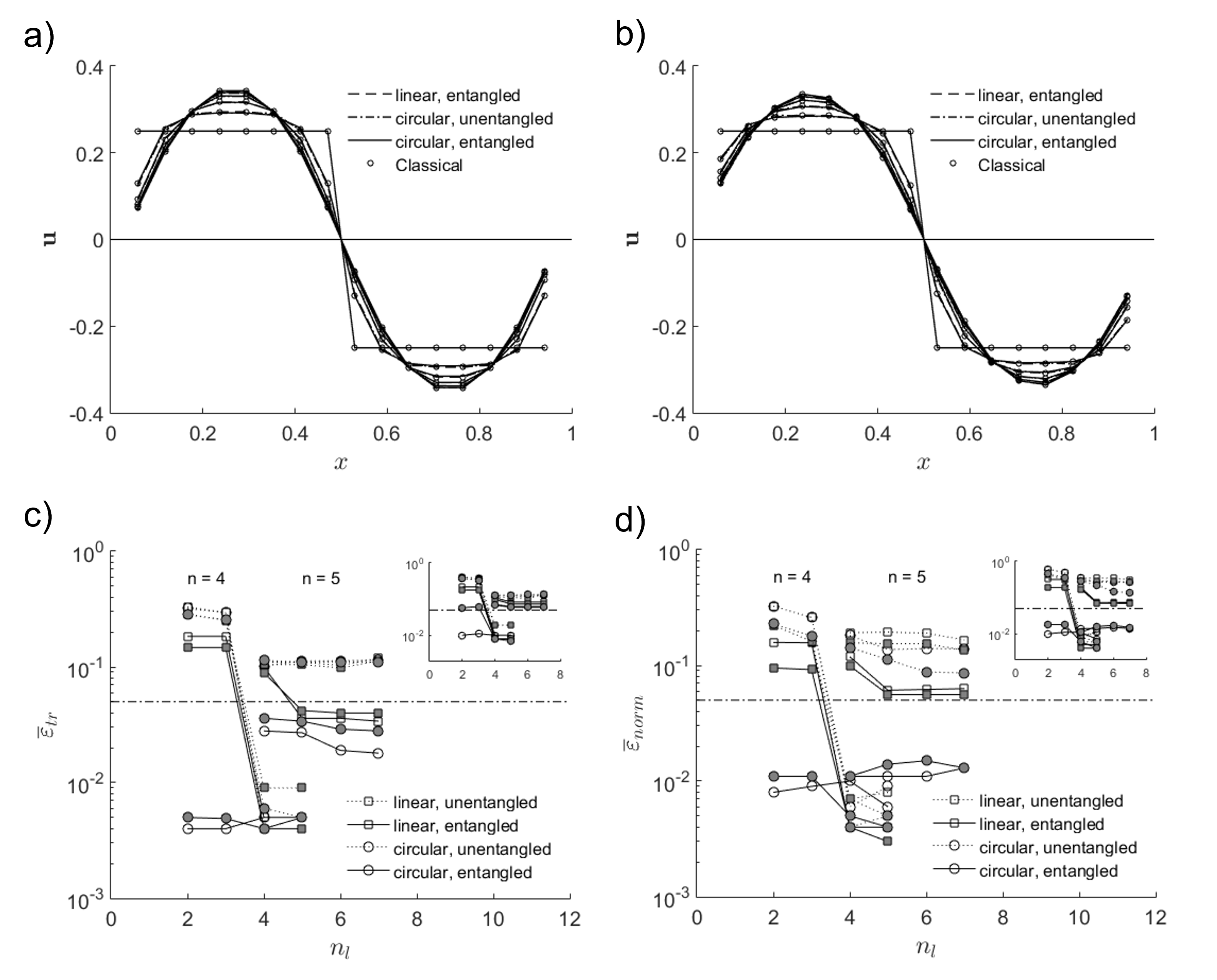
which can be implemented in practice by setting the final parameterized layer $l$ as ${R_{Y}\left(-\frac{\pi}{2}\right)}^{\otimes n}$ with entanglement, or $R_{Y}\left(-\frac{\pi}{2}\right)\otimes{R_{Y}\left(\frac{\pi}{2}\right)}^{\otimes n-1}$ without. Figure 1(a,b) show the time evolution of the step function for four-qubit real-amplitude ansätze with four layers using time-step $\Delta t=10^{-4}$ up to $T=10^{-2}$.

We measure the fidelity of the VQS solution obtained from each ansatz compared to the classical solution, and define the trace error as

$$\varepsilon_{\operatorname{tr}}(t)=\sqrt{1-\left|\langle\widehat{u}_{c}(t)\left|u(t)\right\rangle\right|^{2}},$$ (15)

Similarly, we define the norm error as

$$\varepsilon_{\mathrm{norm}}(t)=\left\lvert 1-\frac{\theta_{0}(t)}{\left\|\mathbf{u}_{c}(t)\right\|}\right\rvert,$$ (16)

where $\theta_{0}(t)$ is the normalization parameter as previously defined. Figure 1(c,d) shows the mean trace and norm errors depending on the number of ansatz layers $n_{l}$ using time-step $\Delta t=10^{-4}$ up to $T=0.01$, for periodic and Dirichlet boundary condition, the latter shown as closed symbols for $\left|\mathbf{f}(t)\right\rangle=0$.

The circular, fully entangled ansatz (Eq. 13d), here termed full circular ansatz for short, was found to outperform other ansätze, requiring fewer parameters for the same solution fidelity. For four qubits, the full circular ansatz is the only one able to produce a solution overlap with only two or three layers, which is less than the minimum required for convergence $n_{l}<2^{n}/n$. For five qubits, it delivered reduced solution and norm errors compared to other ansätze, independent of the number of layers. In this benchmark, the additional term introduced by the Dirichlet boundary condition does not diminish the superior performance of the full circular ansatz.

Refer to caption
Figure 1: Initial step evolves under (a) periodic and (b) Dirichlet boundary condition on a $2^{n}=16$ grid for a real-amplitude ansatz with four layers using time-step $\Delta t=10^{-4}$ plotted in increments of $2\times 10^{-3}$. Mean (c) trace and (d) norm error plotted on a semi-log scale against the number of ansatz layers for various real-amplitude designs under periodic (open symbols) and Dirichlet (closed symbols) boundary conditions up to $T=10^{-2}$ (insets show peak error). The data is grouped into four qubits (two to five layers) and five qubits (four to seven layers). Dash-dot line represents 5% reference error. Source: Figure by authors.

2.4 Initialization

An initial quantum state $|u(0)\rangle$ can be prepared through classical optimization and accepting converged solutions whose norms fall below a specified threshold [alghassi2022, fontanela2021quantum], or direct encoding using quantum generative adversarial networks [Zoufal2019]. In most cases, quantum encoding is cost-prohibitive, and sub-exponential encoding can be achieved only under limiting conditions [Nakaji2022, mitsuda2022approximate].

The Dirac delta function is a popular initial probability distribution found in Fokker-Planck equations [alghassi2022, kubo2021]. To encode the state $|x\rangle$ in the computational basis $\left\{|\boldsymbol{x}\rangle=\bigotimes_{i}^{n}|x_{i}\rangle\right\}$ with $x_{i}\in\left\{0,1\right\}$, one seeks a parameterized ansatz $|\widetilde{u}(\boldsymbol{\theta}(0))\rangle$ for an input state $|0\rangle$.

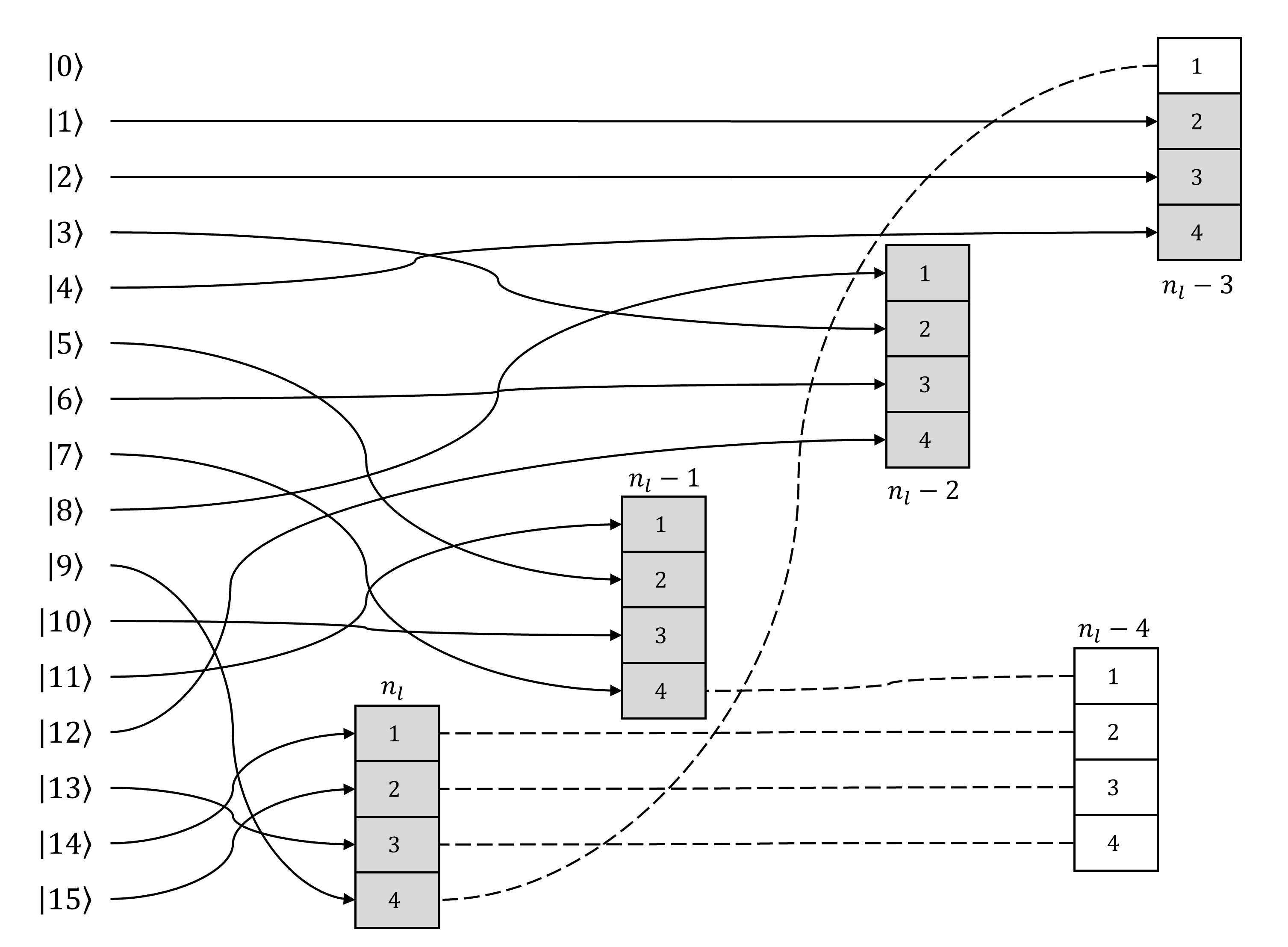
It turns out that for a full circular ansatz (Eq. 13d), encoding $|\boldsymbol{x}\rangle$ does not necessarily require costly optimization. To access a given state $|x\rangle$, one can search for a parameterized layer $n_{l}-k$ such that a $\pi$ bit-flip rotation on an $R_{y}(\theta^{n_{l}-k}_{[1,n]})$ gate (or gates) yields an input state $|x_{0}\rangle$ which transforms to the output state after $k$ circular entangling layers, i.e. $C^{k}_{n}|x_{0}\rangle=|x\rangle$, where the matrix $C_{n}$ represents a single circular entangling layer (Appendix LABEL:sec:B).

Figure 2 shows that for a four-qubit full circular ansatz, all $2^{4}-1=15$ $|x\rangle$ states can be encoded by a single $\pi$ bit-flip rotation of an $R_{y}$ gate within four parameterized layers.

Refer to caption
Figure 2: Mapping state $|x\rangle$ to an input state $|x_{0}\rangle$ at the $n_{l}-k$ layer of a four-qubit full circular ansatz. All $2^{4}-1=15$ $|x\rangle$ states can be mapped within four parameterized layers (grey boxes). For example, $|10\rangle$ can be encoded via a single bit-flip rotation at the $R_{y}(\theta^{n_{l}-1}_{3}=\pi)$ gate, which yields $|x_{0}\rangle=|0100\rangle$ at the $n_{l}-1$ layer. Source: Figure by authors.

2.5 Time Complexity

To assess the time complexity of the VQS algorithm, we estimate the number of quantum circuits required per time step as

$$n_{q}^{\mathrm{VQS}}\approx\left(n_{p}+1\right)\left(\frac{n_{p}}{2}+n_{h}\right),$$ (17)

where $n_{p}$ is the number of ansatz parameters ($n_{p}=n_{l}n$ for a real-amplitude ansatz) and $n_{h}$ is the number of terms in the Hamiltonian (LABEL:eqT12). Likewise, the number of circuits required per time step for a VQE implementation [leong2022Quantum] can be estimated as

$$n_{q}^{\mathrm{VQE}}\approx n_{\mathrm{it}}\left(n_{p}+n_{h}\right),$$ (18)

where $n_{\mathrm{it}}$ is the number of iterations taken by the classical optimizer. Hence, the VQS algorithm is comparable with VQE in terms of circuit counts, if the number of ansatz parameters is roughly double the expected number of iterations required for VQE, i.e. $n_{p}\approx 2n_{\mathrm{it}}\gg n_{h}$.

For each circuit, the time complexity scales as [sato2021variational]

$$t_{q}^{\mathrm{VQS}}\sim\mathcal{O}\left(\frac{d_{\mathrm{ansatz}}+d_{\mathrm{shift}}}{\varepsilon^{2}}\right),$$ (19)

where $d_{\mathrm{ansatz}}\sim\mathcal{O}(n_{l})$ is the depth of the ansatz, $d_{\mathrm{shift}}\sim\mathcal{O}(n^{2})$ is the depth of the shift operator, and the denominator $\mathcal{O}(\varepsilon^{2})$ reflects the number of shots required for estimated expectation values up to a mean squared error of $\varepsilon^{2}$. Another consideration is the depth for amplitude encoding $d_{\mathrm{enc}}$, which can range from $\mathcal{O}(n^{2})$ to $\mathcal{O}(2^{n})$. For VQS, encoding is performed once during initialization, but unlike VQE, repeated encoding is not necessary for time-stepping [leong2022Quantum].

To solve an evolution PDE (e.g. LABEL:eqT1), a classical algorithm iterates a matrix of size $2^{n}\times 2^{n}$, compared to a $n_{p}\times n_{p}$ matrix for VQS, suggesting comparable performance at $n_{l}\approx 2^{n}/n$.

3 Colloidal Transport

With the VQS framework in place, one can explore applications in solving PDEs, such as heat, Black-Scholes and Fokker-Planck equations listed in [alghassi2022]. In this study, we focus on colloidal transport as an application of choice, as the governing Smoluchowski equation involves deep interaction potential energy wells which can be modelled as a component of the Hamiltonian operator (LABEL:eqT10), an aspect oft-neglected in quantum simulations.

3.1 Smoluchowski equation

Consider a spherical colloidal particle of radius $a$ near a planar wall [TorresDiaz2019]. The generalized Smoluchowski equation [Smoluchowski1916] describes the probability $p(h,t)$ of locating the particle at $h$, the distance of the particle center from the wall at time $t$, as

$$\frac{\partial p\left(h,t\right)}{\partial t}=\nabla\cdot D\left(\nabla+\nabla U(h)\right)p\left(h,t\right),$$ (20)

where $D$ is the diffusivity matrix. $U(h)$ is the Derjaguin-Landau-Verwey-Overbeek (DLVO) sphere-wall interaction energy [bhattacharjee1998dlvo], which is the sum of the electric double-layer and van der Waal’s interaction energies, expressed as

$$\boldsymbol{U}=Ze^{-\kappa H}-\frac{A}{H},$$ (21)

where $\boldsymbol{U}=U(h)$ and $H=(h-a)/a$ is the dimensionless separation distance between the particle and wall. The electric double-layer coefficient, normalized inverse Debye length and van der Waal’s coefficient are respectively,

$\displaystyle\begin{gathered}Z=\frac{64\pi\varepsilon\varepsilon_{0}ak_{\mathrm{B}}T}{\left(z_{v}e\right)^{2}}\tanh{\left(\frac{z_{v}e\zeta_{p}}{k_{\mathrm{B}}T}\right)}\tanh{\left(\frac{z_{v}e\zeta_{w}}{k_{\mathrm{B}}T}\right),}\\ \kappa=a\sqrt{\frac{2\left(z_{v}e\right)^{2}I}{\varepsilon\varepsilon_{0}k_{\mathrm{B}}T}},\\ A=\frac{A_{\mathrm{H}}}{6k_{\mathrm{B}}T},\end{gathered}$ (25)

where $\varepsilon$ is the relative permittivity of the medium, $\varepsilon_{0}$ is the permittivity of free space, $z_{v}$ is the ionic valence, $e$ is the electron charge, $k_{\mathrm{B}}$ is the Boltzmann’s constant, and $T$ is the temperature. $\zeta_{p}$ and $\zeta_{w}$ are the zeta potentials on the colloidal particle and wall respectively. $I$ is the ionic strength and $A_{\mathrm{H}}$ is the Hamaker constant.

With that, the first and second derivatives of the interaction energy in separation distance are

$\displaystyle\begin{gathered}\boldsymbol{U}^{\prime}=-Z\kappa e^{-\kappa H}+\frac{A}{H^{2}},\\ \boldsymbol{U}^{\prime\prime}=Z\kappa^{2}e^{-\kappa H}-\frac{2A}{H^{3}}.\\ \end{gathered}$ (29)

Rescaling time $\tau=tD/a^{2}$, we rewrite Eq. 20 in dimensionless form, which gives the evolution of the probability $\boldsymbol{p}(\tau)=p(H,\tau)$ as

$$\frac{\partial\boldsymbol{p}(\tau)}{\partial\tau}=\frac{\partial^{2}\boldsymbol{p}(\tau)}{\partial H^{2}}+\boldsymbol{U}^{\prime}\frac{\partial\boldsymbol{p}(\tau)}{\partial H}+\boldsymbol{U}^{\prime\prime}\boldsymbol{p}(\tau),$$ (30)

which follows from LABEL:eqT1 where $\mathfrak{a}=1$, $\mathfrak{b}=\boldsymbol{U}^{\prime}$, $\mathfrak{c}=\boldsymbol{U}^{\prime\prime}$ and $\mathfrak{f}=0$. Suitable boundary conditions are the absorbing condition on the surface at $\boldsymbol{p}\left(0\right)=0$ (Dirichlet) and the no-flux condition in the far field $\partial\boldsymbol{p}\left(\infty\right)/\partial H\rightarrow 0$ (Neumann) [TorresDiaz2019].

Substituting ${\boldsymbol{p}}(\tau)=\boldsymbol{\rho}(\tau)e^{-\boldsymbol{U}/2}$ [fontanela2021quantum], we express in Dirac notation,

$$\frac{\partial}{\partial\tau}\left|\left.{\rho}\left(\tau\right)\right\rangle\right.=\mathcal{H}\left|\left.\rho\left(\tau\right)\right\rangle\right.,\ \ \left|\left.\rho\left(0\right)\right\rangle\right.=\left|\left.\rho_{0}\right\rangle\right.,$$ (31)

with the Hamiltonian operator

$$\mathcal{H}=\frac{\partial^{2}}{\partial H^{2}}+\boldsymbol{\varphi}^{T}\circ\mathbb{I},$$ (32)

and the potential term

$$\boldsymbol{\varphi}=\frac{{\boldsymbol{U}}^{\prime\prime}}{2}-\left(\frac{{\boldsymbol{U}}^{\prime}}{2}\right)^{2},$$ (33)

which can be evaluated classically (Eq. 29) and implemented as a quantum observable $\boldsymbol{\varphi}^{T}\circ\mathbb{I}$. With Dirichlet-Neumann boundary conditions enforced, the Hamiltonian operator is decomposed as

$\displaystyle\begin{split}\mathcal{H}&=\left[\boldsymbol{\varphi}-\frac{1}{\Delta x^{2}}(\textbf{1}-e_{2^{n}})\right]^{T}\circ\underbrace{I^{\otimes n}}_{H_{1}}+\frac{1}{\Delta x^{2}}\Bigg{\{}\underbrace{I^{\otimes n-1}\otimes X}_{H_{2}}+S^{\dagger}\bigg{[}-\underbrace{I^{\otimes n}}_{H_{3}}+\underbrace{I^{\otimes n-1}\otimes X}_{H_{4}}-\underbrace{I^{\otimes n-1}_{0}\otimes X}_{H_{5}}\bigg{]}S\Bigg{\}},\end{split}$ (34)

where $e_{2^{n}}=(0,0,\ldots,0,1)$.

3.1.1 Potential-free case $(\boldsymbol{\varphi}=\boldsymbol{0})$

Consider first the potential-free case where colloid-wall interactions are absent ($\varphi=0$). The probability density state evolves in space $H\in\left[0,1\right]$ and time $\tau\in\left[0,T\right]$ as

$$\frac{\partial}{\partial\tau}|\rho(\tau)\rangle=\frac{\partial^{2}}{\partial H^{2}}|\rho(\tau)\rangle,\ \ |\rho(0)\rangle=|\rho_{0}\rangle,$$ (35)

where the initial impulse state is centered at $|\rho_{0}\rangle=|2^{n-1}\rangle$. Using a full circular ansatz with 6–8 layers, we evolve the initial pulse on a $2^{n}=16$ grid using time-step $\Delta\tau=10^{-4}$ for early times up to ${10}^{-2}$ (Fig. 3a) and late times up to $T={10}^{-1}$ (Fig. 3b). The former is characterized by the spreading of the probability density due to diffusion, and the latter by the constraints imposed by the asymmetric boundary conditions, which reduces solution fidelity.

To assess the costs of over-parameterization, we calculate the mean trace error (Fig. 3c) and norm error (Fig. 3d) depending on the total number of circuits required $N_{q}$ for the VQS with a run-time of $T={10}^{-1}$. Fig. 3c shows that the mean trace error is insensitive to number of ansatz layers up to six and time-steps up to $5{\times 10}^{-4}$; it is reduced only with further increase in the number of ansatz layers $n_{l}>6$, leading to optimal scaling of ${\bar{\varepsilon}}_{\mathrm{tr}}\sim N_{q}^{-2}$. Closed symbols show results using a higher-order Runge-Kutta time-stepping in place of first-order Euler time-stepping (LABEL:eqT9). We see that the cost scaling of the mean trace error is relatively unaffected by higher-order time-stepping, due to the additional circuit count required for four Runge-Kutta iterations per time-step. The peak trace errors follow a weaker scaling of $\max\left(\varepsilon_{\operatorname{tr}}\right)\sim N_{q}^{-0.8}$.

Refer to caption
Figure 3: Normalized colloidal probability density $\widehat{\rho}(H)$ profiles without interaction ($\boldsymbol{U}=0$) on a $2^{n}=16$ grid using time-step $\Delta\tau=10^{-4}$ plotted in increments of (a) $2\times 10^{-3}$ and (b) $2\times 10^{-2}$ up to $T=10^{-1}$. Lines show VQS solutions based on full circular ansatz with 6–8 layers, and circles show classical solutions based on the same discretization. Mean (c) trace and (d) norm errors plotted on log scale vs. the total number of circuits ${N}_{q}$ for run-time up to ${T}=10^{-1}$ (insets show peak values). Data are grouped by the number of ansatz layers, each set using time-step $\Delta\tau\in\{10,5,2,1\}\times 10^{-4}$. Closed symbols represent Runge-Kutta solutions using time-step $\Delta\tau\in\{10,5,2\}\times 10^{-4}$. Horizontal reference line: $0.05$. Source: Figure by authors.

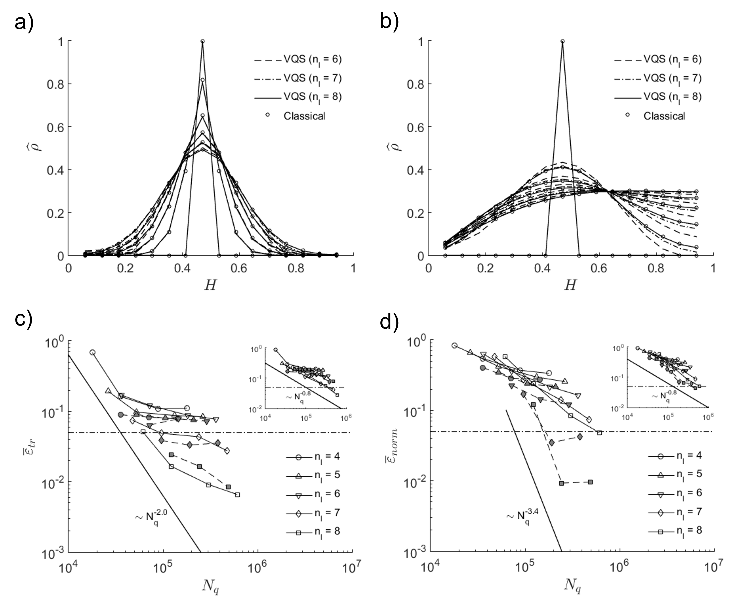
Using Euler time-stepping, the mean norm error scales as $\bar{\varepsilon}_{\mathrm{norm}}\sim N_{q}^{-0.8}$, regardless of $n_{l}$ (Fig. Fig. 3d). This cost scaling improves significantly up to $\bar{\varepsilon}_{\mathrm{norm}}\sim N_{q}^{-3.4}$ using Runge-Kutta time-stepping for circuits with $n_{l}>6$. Note however that this improvement does not extend to the peak norm errors, whose cost scaling remain as $\max(\varepsilon_{\mathrm{norm}})\sim N_{q}^{-0.8}$, regardless of time-stepping scheme.

3.1.2 DLVO potential $\boldsymbol{\varphi}(A,Z,\kappa)$

In the presence of colloid-wall interactions, the DLVO potential term $\varphi$ depends minimally on three parameters, specifically $A$, $Z$ and $\kappa$ (Eq. 25). Following the potential-free case ($n=4,H\in\left[0,1\right],\Delta\tau=10^{-4}$), we perform VQS including $\varphi$ using 8 ansatz layers in time $\tau\in\left[0,T\right]$.

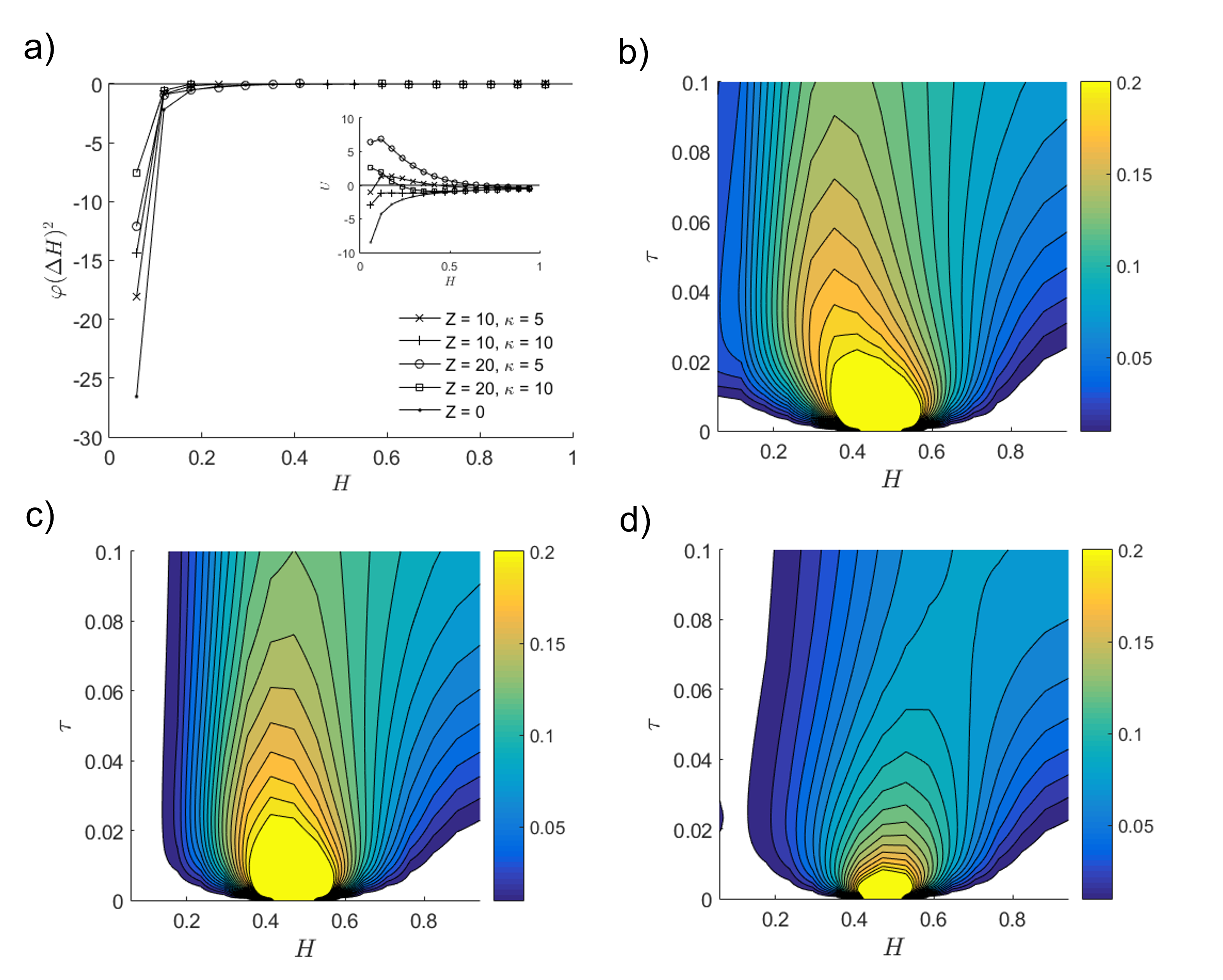
In the absence of the electric double layer $(Z=0)$, the DLVO potential $\varphi(A)$ depends on only the van der Waal’s interaction energy, assumed here to be attractive. Figure 4a shows that the DLVO potential $\varphi(H)$ profiles scaled by the square of the interval $\Delta H^{2}$ for $A\in\{0.05,0.1,0.2,0.5\}$ is only short-ranged in $H$, so the quantum solution $|\rho\rangle$ is insensitive to $A$. Recall however the earlier substitution ${\boldsymbol{p}}(\tau)=\boldsymbol{\rho}(\tau)e^{-\boldsymbol{U}/2}$, such that the actual solution $p$ depends on the longer-ranged interaction energy $\boldsymbol{U}(H)$ (Eq. 21) as shown in Fig. 4a (inset). Indeed, space-time plots show that the colloidal probability density $p(H,\tau)$ for $A=0.05$ up to $T=0.1$ is depleted near wall (Fig. 4c) compared to the potential-free ($\varphi=0$) case (Fig. 4b). Increasing $A$ further increases the depletion range (Fig. 4d).
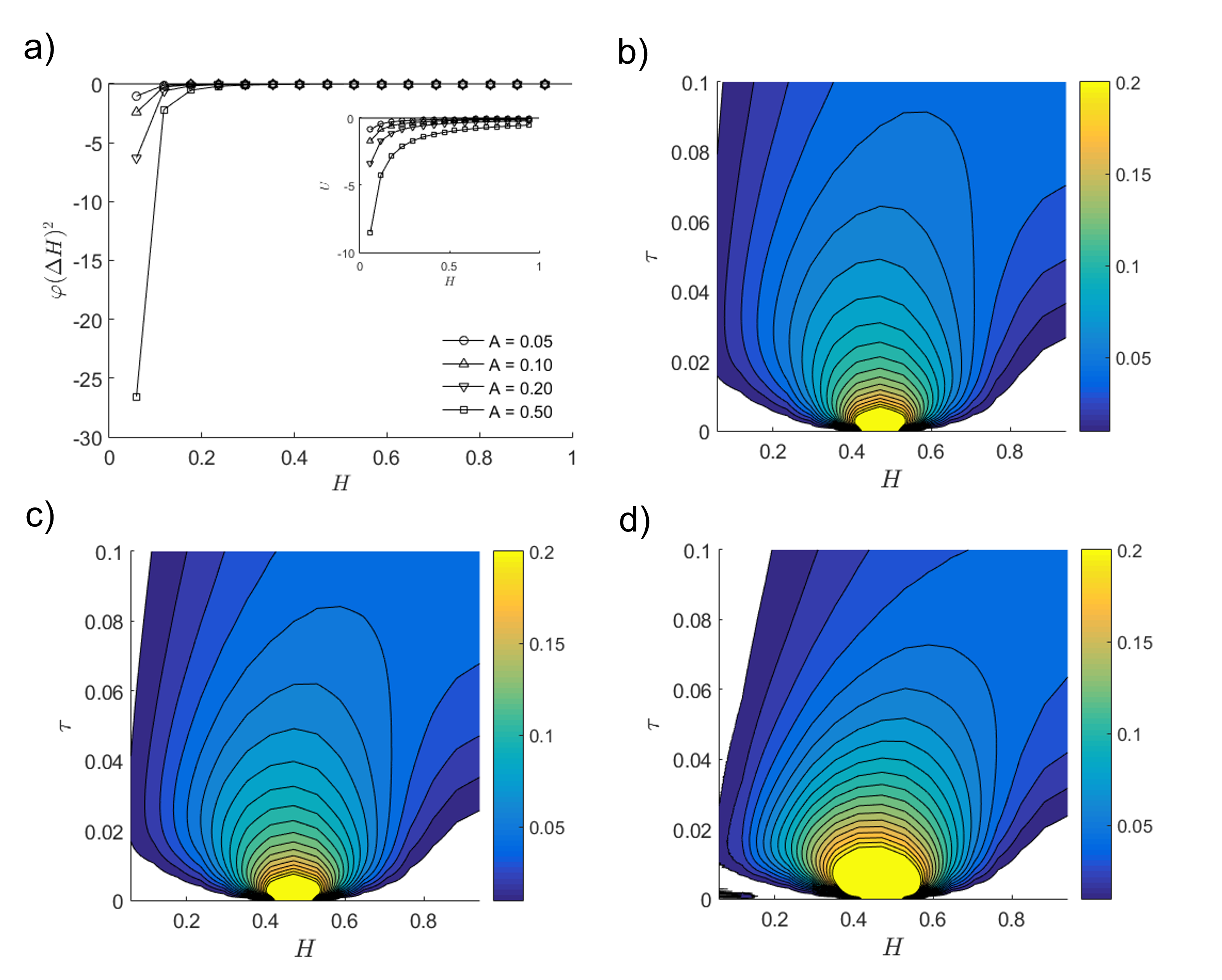
Refer to caption
Figure 4: (a) DLVO potential $\varphi(H)$ profiles scaled by $\Delta H^{2}$ using a full circular ansatz with 8 layers for $Z=0$ varying $A$. Inset shows interaction energy $\boldsymbol{U}(H)$. (b–d) Space-time plots of colloidal probability density $p(H,\tau)\in[\Delta p,0.2]$ with contour interval $\Delta p=0.01$. Given $Z=0$, (b) $\varphi=0$, (c) $A=0.05$ and (d) $A=0.5$. Source: Figure by authors.

Otherwise, the DLVO potential $\varphi(A,K,\kappa)$ includes the electric double layer interaction energy, assumed here to be repulsive. For $A=0.5$, Fig. 5a shows that the DLVO potential shows short-ranged dependence on $Z$ and $\kappa$. However, $p$ depends on the longer-ranged interaction energy $\boldsymbol{U}(H)$ that can be either attractive or repulsive as shown in Fig. 5a (inset). A space-time plot of the colloidal probability density $p(H,\tau)$ for $\{Z,\kappa\}=\{10,10\}$ shows long-ranged influence of the electric double-layer interaction. Parametric analyses of $\{Z,\kappa\}$ holding $A=0.5$ shows that $Z$ depletes $p(H,\tau)$ near wall (Fig. 5c), and a decrease in $\kappa$ increases the deposition flux and depletion range (Fig. 5d).

Refer to caption
Figure 5: (a) DLVO potential $\varphi(H)$ profiles scaled by $\Delta H^{2}$ using a full circular ansatz with 8 layers with $A=0.5$ varying $Z$ and $\kappa$. Inset shows interaction energy $\boldsymbol{U}(H)$. (b–d) Space-time plots of colloidal probability density $p(H,\tau)\in[\Delta p,0.2]$ with contour interval $\Delta p=0.01$. Given $A=0.5$, $\{Z,\kappa\}$ are (b) $\{10,10\}$, (c) $\{20,10\}$ and (d) $\{10,5\}$. Source: Figure by authors.

3.1.3 Trace and norm errors

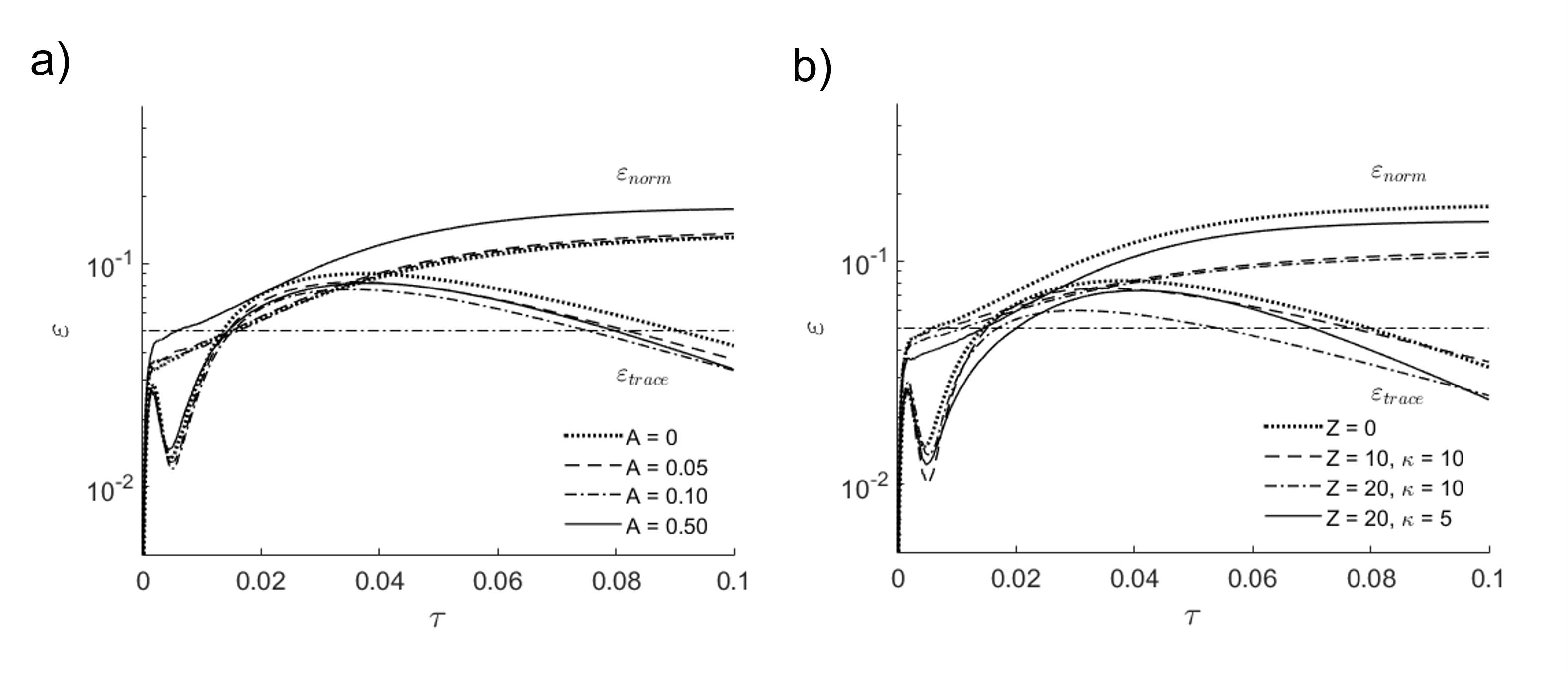
Here we characterize the effect of DLVO potential on the solution fidelity in time using the trace error $\varepsilon_{\mathrm{trace}}(\tau)$ (Eq. 15) and the norm error $\varepsilon_{\mathrm{norm}}(\tau)$ (Eq. 16). Figure 6 shows that $\varepsilon_{\mathrm{trace}}(\tau)$ peaks and decreases during the early diffusion phase (Fig. 3a), then peaks and decreases again as the normalized probability density $\widehat{\rho}$ approaches a steady state profile constrained by the imposed asymmetric boundary conditions (Fig. 3b). Parametric analyses suggest that the electric double layer coefficient $Z$ has the strongest effect on $\varepsilon_{\mathrm{trace}}(\tau)$ (Fig. 6b). In contrast, $\varepsilon_{\mathrm{norm}}(\tau)$ tends towards a steady state regardless of the evolution of probability density. Parametric analyses suggest that $\varepsilon_{\mathrm{norm}}$ is affected by the local depletion of $\widehat{\rho}$ but insensitive to the magnitudes of $A$ (Fig. 6a) and $Z$ (Fig. 6b).

Refer to caption
Figure 6: Trace error $\varepsilon_{\mathrm{trace}}$ and norm error $\varepsilon_{\mathrm{norm}}$ in time $\tau$ for (a) $Z=0$, varying $A$, and (b) $A=0.5$, varying $Z$ and $\kappa$. Horizontal reference line: $0.05$. Source: Figure by authors.

Thus concludes our analysis of the potential term in Eq. 34 in Smoluchowski equation. What usually follows are calculations of survival probability, the probability that the colloidal particle has not reached the wall, and the mean first passage time distribution, the mean rate of change of survival probability. Since they do not involve any quantum computation, they are outside the scope of this study. Interested readers are referred to [TorresDiaz2019].

3.2 Einstein-Smoluchowski equation

The general PDE introduced in LABEL:eqT1 includes a non-homogeneous source term $\boldsymbol{f}$, which is not admissible in Smoluchowski’s description of colloidal probability density. To explore the effects of a source term, we switch over to the analogous Einstein-Smoluchowski equation [Cejas2019, Leong2023],

$$\frac{\partial c\left(h,t\right)}{\partial t}=\nabla\cdot D\left(\nabla+\nabla\boldsymbol{U}\left(h\right)\right)c\left(h,t\right),$$ (36)

which describes the concentration of colloidal particles $c(h,t)$ instead of probability density, but is otherwise identical to the Smoluchowski equation (Eq. 20). The difference here is that a continuous concentration source can be imposed as a far-field Dirichlet boundary condition. Rescaling $c(H,\tau)$ in space $H\in[0,1]$ and time $\tau\in[0,T]$, we perform a change of variables ${\boldsymbol{c}}(\tau)=\boldsymbol{\varsigma}(\tau)e^{-\boldsymbol{U}/2}$ as before, and write

$$\frac{\partial}{\partial\tau}\left|\left.{\varsigma}\left(\tau\right)\right\rangle\right.=\mathcal{H}\left|\left.\varsigma\left(\tau\right)\right\rangle\right.+\mathcal{F}\left|0\right\rangle,\ \ \left|\left.\varsigma\left(0\right)\right\rangle\right.=\left|\left.\varsigma_{0}\right\rangle\right.,$$ (37)

where the operator $\mathcal{F}=X^{\otimes n}$ imposes a unit source in the far field, increasing the required number of quantum circuits by $n_{p}+1$ (Eq. 17) per time step. The number of additional circuits scales with the number of unitaries required to express $\mathcal{F}$.

3.2.1 Initialization

We seek a parameterized ansatz that encodes a Heaviside step function centered at $|2^{n-1}\rangle$,

$$\left|\varsigma_{0}\right\rangle=\left(X\otimes H^{\otimes n-1}\right)\left|0\right\rangle.$$ (38)

For a full circular ansatz (Fig. 13d), this can be encoded on a minimum of two $R_{Y}$ parameterized layers by setting the final layer as $\theta^{n_{l}}_{[1,n]}=\frac{\pi}{2}$ and the second $R_{Y}$ of the preceding layer as $\theta^{n_{l}-1}_{2}=\frac{(-1)^{n-1}\pi}{2}$, where a reversal in the sign produces a step-down function instead.

3.2.2 Solutions and errors
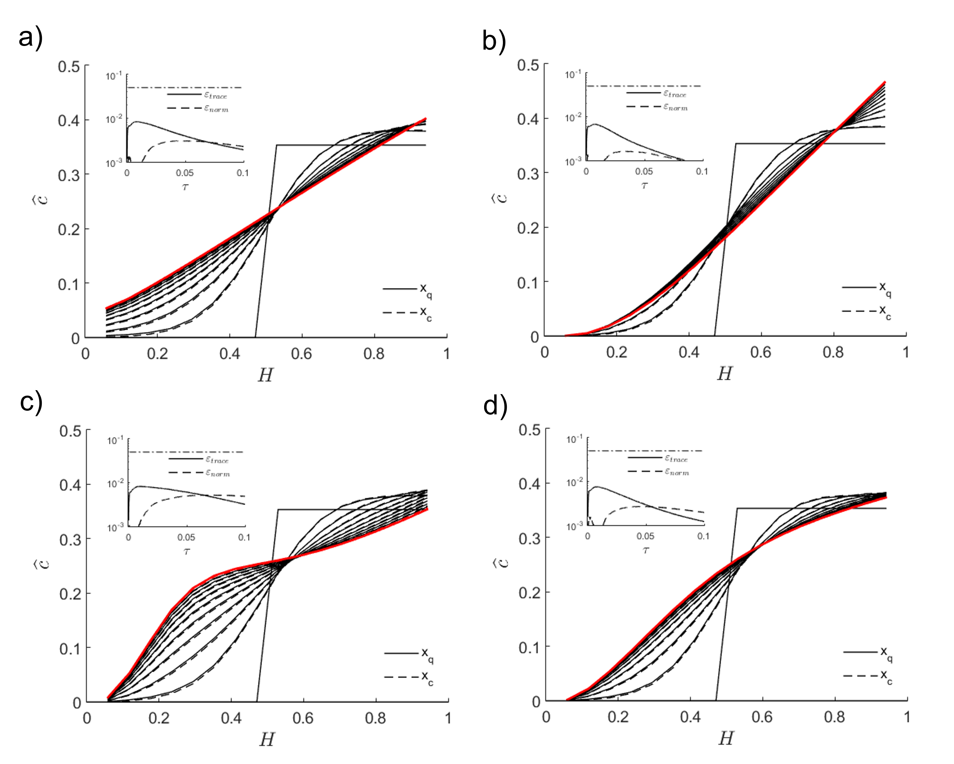
We perform VQS on a $2^{n}=16$ grid using time-step $\Delta\tau=10^{-4}$ as before, but on a full circular ansatz with 5 layers, which is already shown to yield high-fidelity solutions (Fig. 1c,d). Figure 7a shows how the normalized concentration $\widehat{c}$ evolves from the initial step function for the potential-free case ($\boldsymbol{U}=0$). In the absence of an electric double layer ($Z=0$), strong attractive van der Waal’s energy leads to fast convergence towards steady state profile (Fig. 7b). Increasing $Z$ shifts the steady state concentration profile near wall (Fig. 7c) whereas decreasing $\kappa$ increases the depletion range (Fig. 7d). Both trace and norm errors (Fig. 7 insets) decay in time $\tau$ towards convergence with $\varepsilon_{\mathrm{trace}}$ peaking earlier than $\varepsilon_{\mathrm{norm}}$.

Refer to caption
Figure 7: Normalized colloidal concentration $\widehat{c}(H)$ profiles on a $2^{n}=16$ grid using time-step $\Delta\tau=10^{-4}$ plotted in increments of $10^{-2}$ up to $T=10^{-1}$ (bold red). Lines show VQS solutions based on the full circular ansatz with 5 layers. (a) $\boldsymbol{U}=0$ and (b) $A=0.05,Z=0$. Given $A=0.05$, (c) $Z=20,\kappa=10$ and (d) $Z=10,\kappa=5$. Insets show trace error $\varepsilon_{\mathrm{trace}}$ and norm error $\varepsilon_{\mathrm{norm}}$ in time $\tau$. Horizontal reference line: $0.05$. Source: Figure by authors.

4 Conclusion

Currently, neither variational quantum optimization nor simulation is capable of realizing an advantage for solving PDEs over classical methods [Anschuetz2022], but that gap is closing fast [tosti2022review]. For VQS, significant progress has been made since the advent of imaginary time evolution [mcArdle2019variational] notably in the field of quantum finance [kubo2021, fontanela2021quantum, miyamoto2021pricing].

Here we list a formal approach to solving a 1D evolution PDE (LABEL:eqT1):

  • $\{\partial_{t}\boldsymbol{u}(t),\partial_{xx}\boldsymbol{u}(t)\}$ terms handled using variational quantum imaginary time evolution.

  • $\partial_{x}\boldsymbol{u}(t)$ term eliminated through substitution methods, such as $\boldsymbol{u}(t)=e^{g}\boldsymbol{v}(t)$.

  • $\boldsymbol{u}(t)$ term included in the Hamiltonian $\mathcal{H}$ without additional complexity cost.

  • $\boldsymbol{f}(t)$ term realized by an additional set of complementary circuits, whose complexity depends on $\mathcal{F}$.

Superior performance of VQS is contingent on two factors: selection of ansatz and initialization of parameters. Comparing real-amplitude ansatze (Sec. LABEL:sec2.3), we found that the full circular ansatz significantly outperformed not only linear entangled ansatze, but also the popular circularly entangled ansatz but with the final parameterized layer unentangled [alghassi2022, kubo2021]. The advantage in solution fidelity persists over multiple parametric layers, which suggests that unentangled parameterized gates reduce overlap with quantum states that are characteristic of PDE solutions. For an initial state resembling a Dirac delta function (Sec. 2.4), we found that full circular ansatz can be mapped parametrically to a desired state $|x\rangle$, thus reducing subsequent impulse encodings to only a trivial lookup.

As a proof-of-concept, we performed VQS to simulate the transport of colloidal particle to an absorbing wall as described by the Smoluchowski equation (Sec. 3.1), and found high solution fidelity during the initial spreading of the probability distribution. However, to satisfy the asymmetric boundary conditions, additional parameter layers are required, for example up to 6-8 layers for a four-qubit problem. Higher order time-stepping such as Runge-Kutta method can reduce norm errors more effectively than over-parameterization for the same time complexity.

With near-wall DLVO potentials, we found that the van der Waal’s interaction impacts VQS mainly through the potential $\varphi(A)$ of the Hamiltonian, whereas the electric double layer interaction affects the solution mainly through the factor $e^{-\boldsymbol{U}/2}$ obtained from change of variables. Simulations of colloidal concentration with unit boundary source in the far field (Sec. 3.2) requires additional circuit evaluations equal to approximately half the number of parameters. Interestingly, this cost is offset by the fact that fewer parameters are required, here for example, 5 layers for a four-qubit problem.

Overall, we find VQS an efficient tool for applications in colloidal transport since DLVO potentials do not incur additional costs in terms of quantum complexity. Compared to VQE [leong2022Quantum], VQS enjoys significant advantages in that it does not require repeated encodings and iterative optimization loops. In terms of scalability, we found that the accuracy of quantum simulation not only depends on the number of qubits, but also on the imposed boundary and the initial conditions. As with other gradient-based neural networks, VQS potentially suffers from barren plateau problems, which are exemplified by vanishing gradients on flat energy landscapes [mcclean2018barren] and exacerbated by quantum circuits with high expressivity [Holmes2022]. Mitigation strategies for barren plateaus remain an active area of research [Patti2021].

Future work can include extension to 2D model for non-spherical colloids [TorresDiaz2019], optimal ansatz architecture [Tang2021] and initial state preparation [Nakaji2022, Zoufal2020]

Appendix A Quantum circuits to evaluate $A$ and $C$

The elements of matrix $A$ (LABEL:eqT6) and vector $C$ (LABEL:eqT7) can be evaluated via sampling the expectation of an observable $Z$ using quantum circuits shown in LABEL:fig:figA1 [Zoufal2021]. The derivative of the trial state $|\tilde{u}(\boldsymbol{\theta}(t))\rangle$ with respect to $\theta_{k}$ is

$\displaystyle\frac{\partial|\tilde{u}(\boldsymbol{\theta}(t))\rangle}{\partial\theta_{k}}=f_{k}\left[\theta_{0}(t)R_{1}(\theta_{1}(t))R_{2}(\theta_{2}(t))\cdots\sigma_{k}R_{k}(\theta_{k})\cdots R_{N}(\theta_{N}(t))\right]|0\rangle,$ (39)

such that for a single-qubit rotation gate $R_{Y}(\theta_{k})=e^{-i\theta_{k}\sigma_{Y}/2}$, the gate derivative $\partial R_{k}(\theta_{k})/\partial\theta_{k}=-(i/2)\sigma_{Y}e^{-i\theta_{k}\sigma_{Y}/2}$ is measurable with coefficient $f_{k}=-i/2$ and a Pauli-Y gate $\sigma_{k}=\sigma_{Y}$ inserted in the trial state. Accordingly, the quantum circuit may incur a global phase $e^{-i\alpha}$, where $\alpha=0$ and $\pi/2$ for $A$ and $C$ respectively, which may be rectified through an additional phase gate222not to be confused with the cyclic shift operator in LABEL:eqT13, also denoted by $S$., $S=\sigma_{Z}^{1/2}$ on the ancilla qubit.

Conversion to HTML had a Fatal error and exited abruptly. This document may be truncated or damaged.