22email: gabriel.mancino.ball@gmail.com
Y. Xu 33institutetext: Department of Mathematical Sciences, Rensselaer Polytechnic Institute, Troy, NY
33email: xuy21@rpi.edu
Variance-reduced accelerated methods for decentralized stochastic double-regularized nonconvex strongly-concave minimax problems
Abstract
In this paper, we consider the decentralized, stochastic nonconvex strongly-concave (NCSC) minimax problem with nonsmooth regularization terms on both primal and dual variables, wherein a network of computing agents collaborate via peer-to-peer communications. We consider when the coupling function is in expectation or finite-sum form and the double regularizers are convex functions, applied separately to the primal and dual variables. Our algorithmic framework introduces a Lagrangian multiplier to eliminate the consensus constraint on the dual variable. Coupling this with variance-reduction (VR) techniques, our proposed method, entitled VRLM, by a single neighbor communication per iteration, is able to achieve an sample complexity under the general stochastic setting, with either a big-batch or small-batch VR option, where is the condition number of the problem and is the desired solution accuracy. With a big-batch VR, we can additionally achieve communication complexity. Under the special finite-sum setting, our method with a big-batch VR can achieve an sample complexity and communication complexity, where is the number of components in the finite sum. All complexity results match the best-known results achieved by a few existing methods for solving special cases of the problem we consider. To the best of our knowledge, this is the first work which provides convergence guarantees for NCSC minimax problems with general convex nonsmooth regularizers applied to both the primal and dual variables in the decentralized stochastic setting. Numerical experiments are conducted on two machine learning problems. Our code is downloadable from https://github.com/RPI-OPT/VRLM.
Keywords: Stochastic optimization, decentralized optimization, minimax problems, variance reduction
Mathematics Subject Classification: 90C15, 90C26, 90C47, 65K05
1 Introduction
In this paper, we consider the following minimax-structured problem
| (1.1) |
where is a smooth, nonconvex strongly-concave (NCSC) function governed by for each . In the special case where is a discrete uniform distribution, we recover the finite-sum problem setting, and without lose of generality, we can assume each involves the same number of scenarios, i.e.,
| (1.2) |
Thus (1.1) encompasses a broad class of problems. We assume and are closed convex functions, often serving as regularizers, hence we refer to (1.1) as a double-regularized minimax problem. Problem (1.1) has received a lot of research attention recently due to its application in many machine learning settings such as adversarial training Goodfellow2014 ; Mingrui2020 , distributionally robust optimization Namkoong2016 ; Wenhan2021 , and reinforcement learning Xin2021 . It has also been used to study fairness in machine learning Nouiehed2019 and improving generalization error foret2021sharpnessaware .
Motivated by scenarios where data are distributed over many different computing devices Xin2021HSGD , we are interested in the case where is owned privately by the -th one among agents that are connected over a communication network . Here, denotes the set of agents and denotes the set of feasible communication links between the agents. We assume the network is connected. Furthermore, in a stochastic setting, we assume that each agent can only access local stochastic gradients, rather than exact gradients. Such a scheme is close to a real-world setting where agents may not have access to a global communication protocol (either due to privacy restrictions Verbraeken2020 or high communication overhead Lian2017 ), nor access to the entire local gradient (e.g., when data arrives in a stream xu2023-PSTORM ).
In order for the agents to collaboratively solve (1.1), each agent will maintain a copy of the primal-dual variable , denoted as . With the introduction of local variables , we can formulate (1.1) equivalently into the following decentralized consensus minimax problem
| (1.3) |
To ensure that the consensus constraint is satisfied for all , agents exchange their information with their 1-hop neighbors via the communication links in . Mathematically, this communication is represented as multiplication with a mixing matrix, , which serves as an inexact averaging operation among the agents.
The efficiency of a method to solve (1.3) will be measured by the number of samples and neighbor communications required to achieve an -accurate solution; see Definition 3.1. We refer to these quantities as sample and communication complexities, respectively. In this work, we propose the VRLM method which serves as a framework for applying state-of-the-art variance-reduction (VR) techniques to achieve low sample and communication complexities when solving (1.3). Our framework is based on a reformulation of (1.3) which allows for exploitation of the strong-concavity of . We summarize our contributions below.
1.1 Contributions
Our contributions are three-fold. They are summarized as follows.
-
•
First, we provide one decentralized method with two VR options for solving stochastic double-regularized NCSC minimax problems in the form of (1.1) or the equivalent form (1.3). Our method is based on a reformulation of (1.3) introduced in xu2023dgdm , by removing the consensus constraint on the dual variable with the introduction of a Lagrangian multiplier. One VR option of our method uses large-batch sampling, while the other needs only samples for each update per agent. To the best of our knowledge, this is the first decentralized stochastic method for solving the structured problem (1.1), while a few existing methods can only be applied to certain special cases; see more details in the section of related work. Compared to most existing decentralized stochastic methods that even can only solve special cases of (1.1), our method can take times larger stepsize, where is the condition number defined in (3.8). This can potentially lead to better empirical performance; see Remark 3.4.
-
•
Second, we show a last-iterate convergence in probability result for our method with the large-batch VR option on solving finite-sum structured problems. Also, we establish complexity results of our method with either VR option to produce an -stationary solution for any given ; see Definition 3.1. Utilizing just a single neighbor communication per iteration, we prove that both versions of our method can achieve a sample complexity of in the general stochastic setting. The small-batch version attains the same communication complexity, while the large-batch one only needs communication rounds. In addition, for the finite-sum structured problem, our method with the large-batch VR option can achieve a sample complexity of and communication complexity of . These complexity results are optimal in terms of the dependence on arjevani2023lower ; lu2021optimal and match the best-known results of decentralized methods for solving special cases of (1.1). Moreover, our complexity results are graph-topology independent in certain regimes; see Remarks 3.4 and 3.5. Furthermore, when specialized to the single-agent setting, i.e., in (1.1), our method also improves over a few state-of-the-art methods for NCSC finite-sum or stochastic minimax problems. With large-batch sampling, our method achieves the same-order complexity result as SREDA Luo2020 , which requires double loops and only applies to the special case of (1.1) with and for a convex set . If samples are available for each update, our method achieves a lower-order complexity than Acc-MDA huang2022accelerated , which needs sample gradients to produce an -stationary solution.
-
•
Third, we verify the performance of our proposed method on two machine learning problems in a real decentralized computing environment. Additionally, we make our code open source at https://github.com/RPI-OPT/VRLM.
1.2 Related work
| Method | Stoch./F.S. | (, ) | S.C. | Samp. Comp. | Comm. Comp. |
| GT-DA Tsaknakis2020 | F.S. | (0, ) | ✓ | ||
| GT-SRVR Xin2021 | F.S. | (0, 0) | ✓ | ||
| PRECISION liu2023precision ¶ | F.S. | (convex, ) | ✓ | ||
| DREAM Chen2022 | F.S. | (0, ) | ✗ | ||
| Stoch. | |||||
| VRLM-STORM† | Stoch. | (convex, convex) | ✓ | ||
| VRLM-SPIDER‡ | F.S. | (convex, convex) | ✓ | ||
| Stoch. |
A few decentralized methods have been proposed for solving minimax problems. However, most of them focus on deterministic or finite-sum structured problems. We list a few representative methods in Table 1.
The recent D-GDMax method xu2023dgdm is very closely related to our proposed method, as both rely on a reformulation of (1.3) by the introduction of a Lagrangian multiplier to facilitate convergence. A key difference is that D-GDMax requires exact gradients. Thus it is not applicable to the general stochastic problem setting that we consider. Though D-GDMax can be applied to the special finite-sum case, its complexity will be significantly higher than ours if is big and the desired accuracy is small. GT-DA Tsaknakis2020 is also a deterministic gradient method. It solves a variant of (1.3) by only enforcing consensus on either the or variables, but not both simultaneously.
The PRECISION method in liu2023precision is designed for solving (1.3) under the finite-sum setting, and in addition, it assumes for some convex set . Similar to one option of our method, it utilizes the SPIDER-type fang18spider variance reduction. In order to produce an -accurate point, it needs samples and communications rounds without giving an explicit dependence on the problem’s condition number ; the dependence on and is the best-known for the finite-sum setting. A preceding method of PRECISION, called GT-SRVR in Xin2021 , considers a more special case of (1.3) under the finite-sum setting. It assumes and and achieves the same-order complexity results by the SPIDER-type variance reduction. DSGDA Gao2022 solves the same-structured problem as GT-SRVR and also enjoys the same-order complexity results. Different from GT-SRVR, DSGDA uses a SAGA-type acceleration technique defazio2014saga . It does not need to take large-batch samples for each update but requires a large memory to maintain component gradients.
Like our method, DREAM Chen2022 can be applied to both the stochastic and finite-sum settings of (1.3). It employs a loopless version of the SPIDER-type VR method. However, it assumes and . In addition, it performs multiple communications per update, and its convergence results rely on the multi-communication trick. This is fundamentally different from our method. With a multi-communication trick, our results can have a lower-order dependence on the spectral of the communication network; see Remark 3.4. However, we can have guaranteed convergence with a single communication per update, while the analysis of DREAM requires the multi-communication trick to prove convergence. The requirement of multiple communications can be too restrictive and even impractical in a real computing setting, as it needs more coordinations between agents Lian2017 . All the aforementioned methods require either large-batch samplings or a large number of maintained component gradients. In contrast, DM-HSGD Wenhan2021 , by the STORM-type cutkosky2019momentum VR technique, only needs samples per update per agent, except for a possible large-batch sampling at the initial step. However, there is one critical error with its convergence analysis. It turns out that Eqn. (28) in Wenhan2021 does not hold with the given choice of . In fact, must be instead of the given , where is the smoothness constant of and the strong-concavity constant of . With the correct , it is unclear if its final claimed convergence results will hold111With , the coefficient for becomes positive but it is required to be negative in the analysis for DM-HSGD..
All the methods we mentioned above assume strong concavity about the dual variable and also convexity of the regularization terms or constraint sets, if there are any. A few existing decentralized methods for minimax problems make weaker or different assumptions. For example, DPOSG Mingrui2020 is designed to solve smooth stochastic nonconvex nonconcave decentralized minimax problems. Instead of concavity structure, the Minty VI condition is assumed by DPOSG in order to have guaranteed convergence. However, its complexity has a high-order dependence on a given accuracy, reaching to produce an -stationary solution. In addition, it cannot handle problems with nonsmooth regularization terms or a hard constraint. This is another fundamental difference from our method.
Though our focus is on decentralized computation, our method is also applicable in the single-agent (or non-distributed) setting, i.e., the problem (1.1) with . In this case, many methods have been proposed under various settings of . The GDA lin2020gradient method can be applied to dual-constrained smooth deterministic NCSC minimax problems, i.e., and in (1.1). To achieve an -accurate solution, it requires gradient evaluations, which was later reduced to by the Minimax-PPA lin2020near method. When or , proximal-AltGDAm chen2021accelerated can achieve a complexity result of . In the stochastic setting, GDA utilizes large-batch sampling and can achieve a sample complexity of . SREDA Luo2020 considers both stochastic and finite-sum structured minimax problems. Similar to one choice of our method in the single-agent setting, it adopts the SPIDER-type VR. However, different from our method, SREDA needs an inner loop to approximately solve the dual maximization problem, and thus it is a double-loop method. It achieves a sample complexity of for the finite-sum case and for the stochastic case. All aforementioned single-agent methods require a large batch-size: either all samples in a deterministic/finite-sum setting or as many as in a stochastic setting where SPIDER-type VR is used. In contrast, Acc-MDA huang2022accelerated can achieve a complexity of by samples per update through the STORM-type variance reduction. SAPD+ zhang2022sapd can also have convergence guarantees by small-batch sampling and achieves a complexity of . When big-batch sampling is performed, SAPD+ can have a complexity of by variance reduction. However, different from Acc-MDA and our method in a single-agent setting, SAPD+ is a double-loop method. A comprehensive literature review for single-agent methods designed for solving (1.1) is out of the scope of this work. The interested readers can refer to the references therein of previously mentioned works for a more thorough treatment of this subject, including whether or not each method can handle or . For readers interested in works that handle the nonconvex concave or nonconvex nonconcave settings, see e.g., ostrovskii2021efficient ; thekumparampil2019efficient ; zhang2022sapd ; jin2020local ; lin2020gradient ; yang2022faster ; xu2023unified ; zheng2023doubly .
1.3 Notation
We denote as the set . We let and be the joint variable and domain. For each , let be a local copy of on agent . Then we denote
| (1.4a) | |||
| (1.4b) | |||
We use the superscript (t) for the -th iteration. For a set , we denote its indicator function by , i.e., if and otherwise. For a closed convex function , we define its proximal mapping as . Finally, given a set of random samples , we denote
| (1.5) |
1.4 Outline
2 Proposed method
The primary challenges with providing convergence guarantees for decentralized methods that solve (1.3) are caused by the non-linearity of the proximal mapping associated with the non-smooth terms and , the nonconvexity of , and the stochasticity of gradient information.
To address these challenges, we adopt a reformulation of (1.3), introduced in the recent work xu2023dgdm , by using a Lagrangian multiplier to remove the consensus constraint on . Formally, we define
| (2.1) |
such that when has nonempty relative interior, the problem (1.3) can be reformulated equivalently into
| (2.2) |
In addition, we incorporate VR techniques to facilitate a better estimate of the true local gradients. Specifically, we provide convergence guarantees when agents utilize either the SPIDER fang18spider ; nguyen2017sarah or STORM-type cutkosky2019momentum ; xu2023-PSTORM VR technique. By additionally using gradient tracking lorenzo16 ; nedic17 ; songtao19 ; zhang20gradtrack ; koloskova21 in the -variable, we make the least restrictive assumptions on the data distribution among the agents tang18 , namely, heterogeneous data is allowed. Combining all of the above ideas leads to our Variance Reduced Lagrangian Multiplier based method for decentralized double-regularized minimax problems, VRLM. Its pseudocode is summarized in Algorithm 1.
| (2.3) |
| (2.4) |
The updates in (2.3) utilize the SPIDER-type VR technique, which requires large-batch sampling, meaning that the number of samples at each iteration to compute a local gradient estimator depends on a desired solution accuracy . As shown in the next section and in Table 1, the large batches can lead to an improved communication complexity result, but may lead to poor generalization on some machine learning tasks keskar17 . Furthermore, in scenarios where the data arrives in a stream it may be impractical to wait for enough samples to compute a large-batch gradient estimator. Hence, we also allow for agents to utilize the STORM VR technique in (2.4). By the STORM technique, agents only need samples to compute a stochastic gradient estimator, except for a possible large-batch sampling at the initial step. We find in practice (see Section 4) that the STORM estimator outperforms the SPIDER estimator on more complex tasks. Nevertheless, we will provide convergence analysis for both methods.
3 Convergence results
In this section, we give the convergence results of Algorithm 1 for two VR options (by setting the VR-tag in Algorithm 1). The following definitions are used throughout our analysis with given in (2.1).
| (3.1) | |||
| (3.2) | |||
| (3.3) | |||
| (3.4) | |||
| (3.5) |
By Danskin’s theorem Danskin1966 , with , we have
| (3.6) |
The analysis will be conducted based on the following assumptions, which are standard in the minimax and decentralized optimization literature Xin2021 ; shi15 .
Assumption 3.1
The function is -strongly convex with , for each ; there exists such that for all where is defined in (3.2); has a nonempty relative interior.
Assumption 3.2
The mixing matrix satisfies the conditions: and ; ; .
Assumption 3.3
For each , is -smooth. In addition, in the stochastic case, satisfies (i) , (ii) there exists such that , and (iii) for any , it holds .
Throughout this paper, we denote the condition number by
| (3.8) |
To quantify the sample and communication complexities, we are interested in finding a near-stationary point of (2.2), defined below.
Definition 3.1
For any , a random point is called an -stationary point in expectation of (2.2) if there is some such that
| (3.9) |
Remark 3.1
Notice that is the objective function of the primal problem of (2.2). The stationarity measure in Definition 3.1 is sometimes called optimization stationarity zheng2022doubly . Another related notion is the so-called game stationarity, which also involves the dual variable . In addition, xu2023dgdm shows that if is an -stationary point of (2.2), then is an -stationary point of the original decentralized formulation (1.3) when is smooth. This claim can actually be extended to the case where the function defined in (3.1) satisfies a quadratic-growth condition drusvyatskiy2018error for all . Hence, we adopt the notion in Definition 3.1.
3.1 Preparatory results
We begin with the following preparatory propositions. The first one is directly from xu2023dgdm .
Proposition 3.1
Let and be defined in (3.1). Then with , it holds
| (3.10a) | |||
| (3.10b) | |||
| (3.10c) | |||
Proposition 3.2
Let be defined in (3.1). Then with , it holds
| (3.12) |
Proof
The inequality in (3.12) indicates the smoothness of under a weighted norm. By (nesterov2013gradient, , Eqn. 2.12), we have that for any with and any ,
| (3.13) |
3.2 One-iteration progress inequality
Our analysis relies on establishing a one-iteration progress inequality about based on the updates in lines 8-10 in Algorithm 1. Its proof is deferred to Appendix B.
Lemma 3.2
3.3 Consensus and dual error bounds.
The following proof can be found in Lemma C.7 of mancino2022proximal .
Lemma 3.3
Finally, we provide upper bounds to the dual errors. The proofs are given in Appendix C.
Lemma 3.5
3.4 Convergence results by SPIDER-type variance reduction
In this subsection, we set VR-tag = SPIDER in Algorithm 1, and we consider both the general stochastic case and the special finite-sum setting. The proofs of all the lemmas are given in Appendix D. We first bound the consensus error of the tracked gradient and the error of the gradient estimator.
Lemma 3.7
Remark 3.2
Notice that for any , we have . Therefore
| (3.26) |
The relation in (3.26) is standard in the analysis of SPIDER-type methods; e.g., see (xin2021proxgt, , Eqn. (85)).
In the rest of this subsection, we set
| (3.27) |
Lemma 3.8
Below we show the square summability of the generated sequence, which is crucial to obtain our convergence and complexity results.
Theorem 3.1
Proof
We first take the expectation of (3.16), apply (3.19), and plug in the values of and to have
| (3.32) |
where the coefficient of is obtained by the arguments
Next, for any and , we add to both sides of (3.32) and use the results of Lemmas 3.3 and 3.7 to obtain
| (3.33) | ||||
Sum up (3.33) over to , utilize (3.26), and recall to have
| (3.34) | ||||
Now plug (3.28) and (3.29) into (3.4) and also bound by (3.7) to have
| (3.35) | ||||
Set and to
| (3.36) | |||
| (3.37) |
By and , it is straightforward to have . Then we have from (3.36) and (3.37) that
| (3.38) |
In addition, by the choice of in (3.37), it follows
| (3.39) |
By the choice of and , it follows that
| (3.40) |
Also, , and by , it holds
Hence from (3.40), we have . Thus follows from (3.37), and we have
| (3.41) |
where the last inequality can be verified by plugging the value of given in (3.30a). Similarly, by the choice of in (3.30b), it is straightforward to have
| (3.42) |
Moreover, by , it holds
| (3.43) |
Therefore, we obtain (3.1) from (3.4) by using (3.4)-(3.43), the lower bounds and , the upper bounds and , and .
By Theorem 3.1, we first show a last-iterate convergence in probability for the finite-sum case.
Theorem 3.2 (Convergence in probability for finite-sum case)
Proof
Remark 3.3
In order to show the last-iterate convergence in probability for the general stochastic case, we need to increase periodically such that the cumulated variance is finite. This requires us to make dependent on the number of periods, which will cause confusion on the notation. We do not extend the analysis here. In addition, Theorem 3.2 together with Remark 3.1 implies that satisfies the convergence in probability for (1.3) when (1.2) holds and in Algorithm 1, i.e.,
where is defined in (3.2).
Moreover, by Theorem 3.1, we have the expected convergence rate result below.
Theorem 3.3
Proof
By the selection of , we have . Hence, it follows from (3.28) and (3.1) that
| (3.47) | ||||
Similarly, we have from (3.29) and (3.1) that
| (3.48) |
Below we give the total sample and communication complexity result. The proof is given in Appendix D.
Corollary 1
Let be given and assume . Under the same assumptions as in Theorem 3.3, suppose
Then Algorithm 1 with VR-tag = SPIDER, for the general stochastic case and for the special finite-sum case, and can find an -stationary point in expectation of (2.2) by stochastic gradients and local neighbor communications, where
and for the finite-sum case and for the general stochastic case.
Remark 3.4
The assumption on and is mild and can easily hold if is not small. Otherwise, multiple communications can be performed at the initial step to satisfy the condition. In addition, when , the complexity results will be independent of the graph topology. In this case, our stepsize and in (3.30) are both in the order of , matching to that used by a centralized method for NCSC minimax problems, e.g., the GDA in lin2020gradient . This can be significantly larger than the stepsize in the order of taken by state-of-the-art decentralized methods for minimax problems, e.g., PRECISION liu2023precision and DSGDA Gao2022 . When , then linearly depends on , which is worse than existing results with a dependence of for decentralized methods with a single communication per iteration on solving composite nonconvex problems; see scutari2019distributed for example. To improve the dependence, we can again perform multiple communications in the initial step to have . Moreover, if the multi-communication trick, which needs more coordinations between agents, is applied for every update, we can change the mixing matrix in our analysis to a polynomial in , denoted by . If is symmetric, we can apply the Chebyshev polynomial (e.g., see mancino2023decentralized ) to have an accelerated averaging. This way, the sample complexity will be independent of and the communication complexity will linearly depend on .
3.5 Convergence results by STORM-type variance reduction
In this subsection, we set VR-tag = STORM in Algorithm 1. The general proof structure mimics that of Section 3.4. The proofs of all lemmas are given in Appendix E.
Lemma 3.9
In the rest of this subsection, we set
| (3.53) |
With Lemma 3.9, we can use (3.16) to show a result similar to Theorem 3.1.
Lemma 3.10
We have the following convergence rate result by Lemma 3.10.
Theorem 3.4
Proof
Based on Theorem 3.4, we give, in the following corollary, the complexity results of VRLM-STORM. For simplicity, we focus on the high-accuracy regime, i.e., is sufficiently small.
Corollary 2
A few remarks are in order regarding the above corollary.
Remark 3.5
First, similar to other recent works Xin2021HSGD ; mancino2022proximal , our complexity results are stated for the high-accuracy regime (i.e. small enough ). Technically, this accuracy requirement removes the final dependence of VRLM-STORM on the spectrum of the graph. Second, the initialization requirements in Corollary 2 are akin to those in mancino2022proximal . If necessary, e.g., when is much smaller than , we can perform multiple communications at the initial step to have . Third, the recent Acc-MDA huang2022accelerated method can attain a convergence rate of , however, this is only in the single-agent setting where and further, this result only holds when When , we have , which eliminates the variable , as well as the consensus constraint on . Hence, (2.2) is actually identical to (1.1) which indicates our analysis provides a better dependence on , as well proves convergence on a broader class of problems (i.e., and/or ).
4 Numerical experiments
In this section, we empirically validate our proposed methods on two benchmark problems which fit (1.3). We compare our methods to three methods: DPSOG Mingrui2020 , DM-HSGD Wenhan2021 , and GT-SRVR Xin2021 ; since these methods are only presented for the case of (1.3) with , we simply wrap their updates with For our experiments, we use agents, where each agent is an NVIDIA Tesla V100 GPU. The agents are connected via a ring structured graph, where self-weighting and neighbor weighting are . Our code is made available at https://github.com/RPI-OPT/VRLM.
4.1 Sparse distributionally robust optimization
We test our proposed method on the decentralized distributionally robust optimization problem xu2023dgdm using both the MNIST lecun98 and Fashion-MNIST xiao17fashion datasets. Each agent maintains a local dataset, , where is the -th image on the -th agent and is the corresponding label among classes. The total number of data points is given by and we let be an index set which contains the indices of data points on agent . The agents’ local objective functions are given by
| (4.1) |
Here, denotes the -th component of , is the cross-entropy loss function taken over each class, is a neural network governed by the parameter , and is a parameter controling the deviation from the uniform distribution. The set is the standard probability simplex. The regularizer induces sparsity on the variable. We choose to be a two-layer neural network with 200 hidden units and Tanh activation function. Further, we let and .
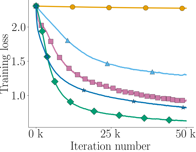
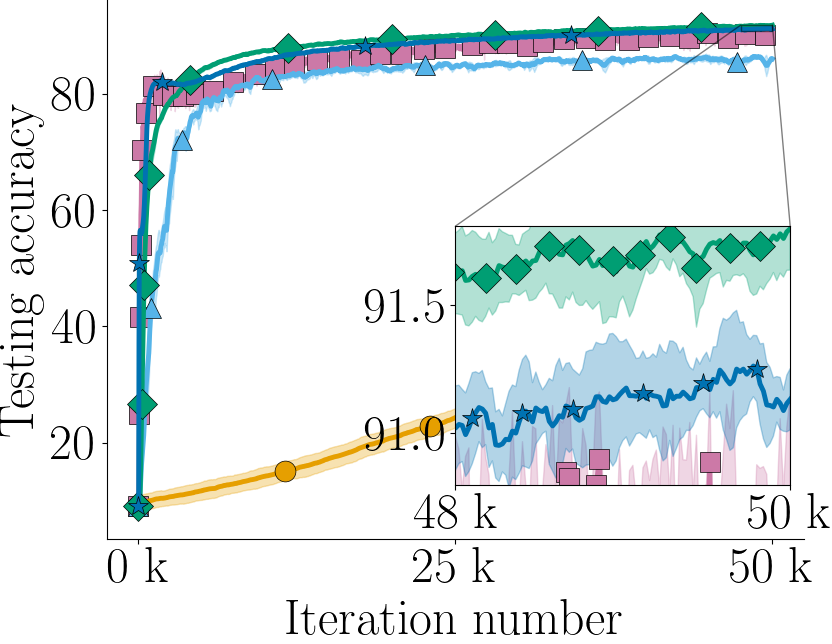
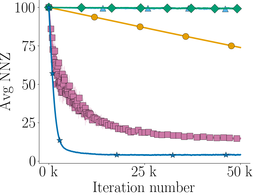
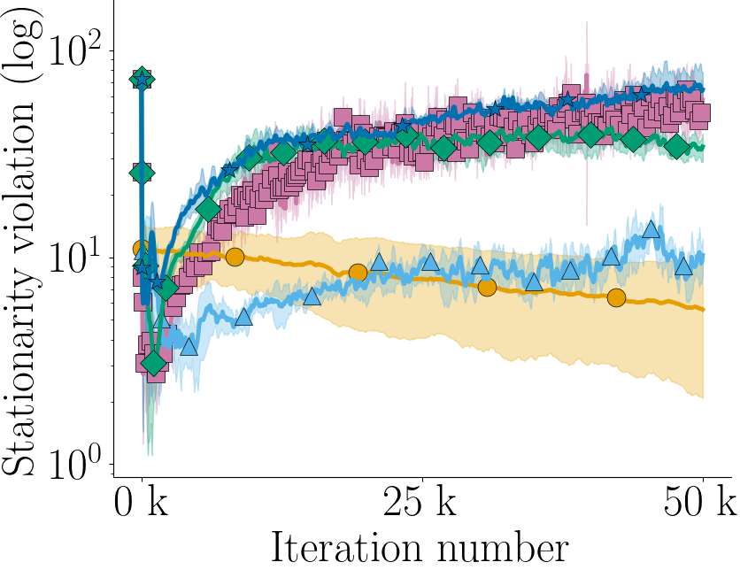
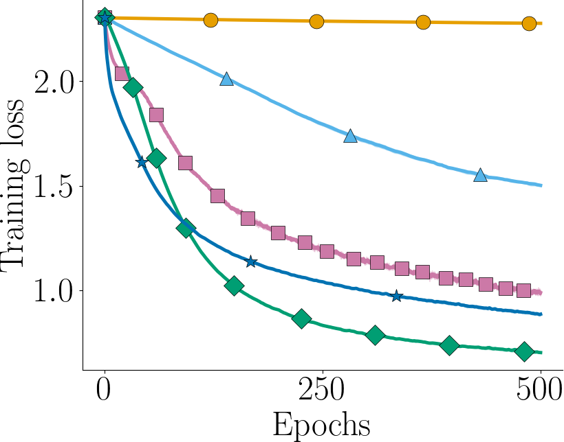
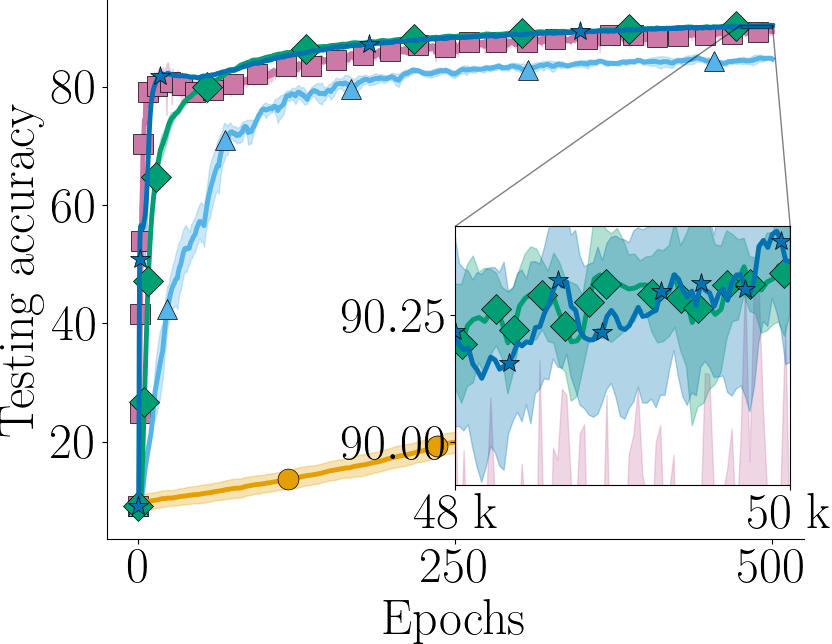
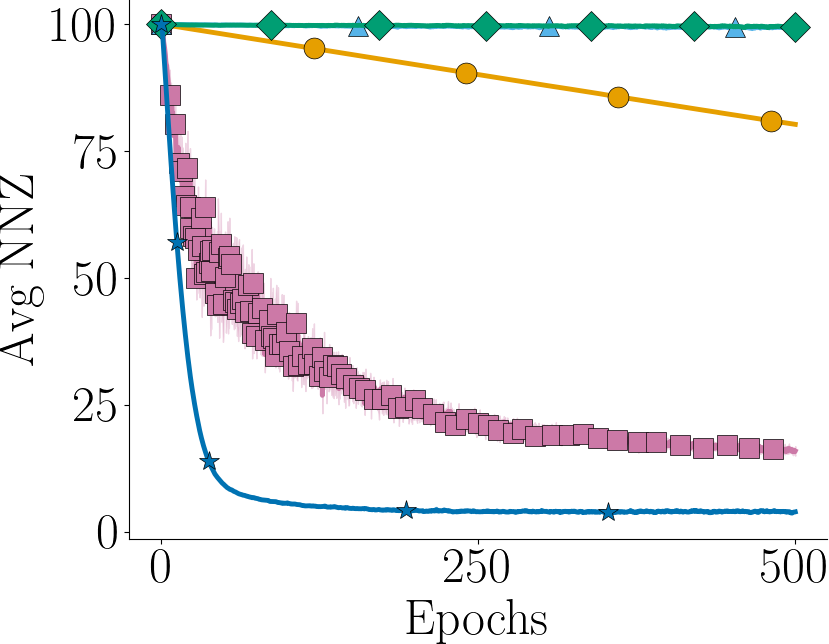
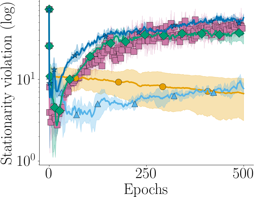
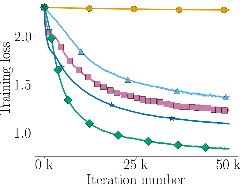
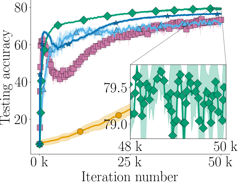
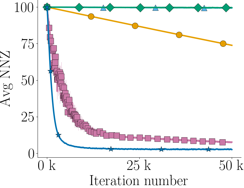
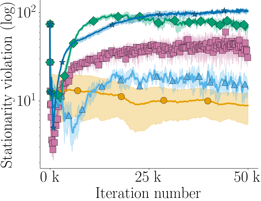
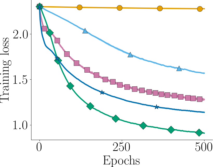
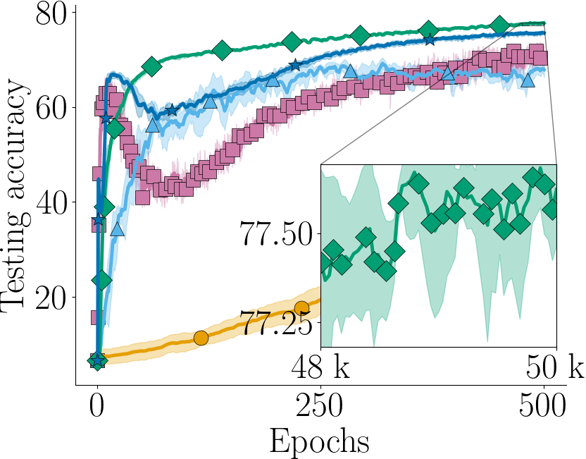
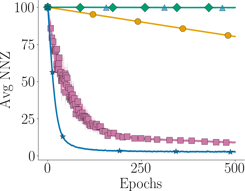
The dataset is split uniformly at random among the agents, hence each agent receives local data points. We let the mini-batch size for all methods be 100 and tune and . For DM-HSGD, we tune following the paper guidelines and set the initial batch-size to 3000. For GT-SRVR, we tune and the large mini-batch size from . For VRLM-STORM we let , , and . For VRLM-SPIDER, we tune and the large mini-batch size from and let and . We run all methods to iterations and compare the training loss value (as if performing centralized training; note this is not the objective value), testing accuracy, average number of non-zeros, and stationarity violation, where the stationarity violation is computed as
| (4.2) |
where for . We run each experiment with 5 different initial seeds and report the average results across both iterations and epochs.
 |
 |
 |
 |
 |
 |
 |
 |
 |
 |
 |
 |
 |
 |
 |
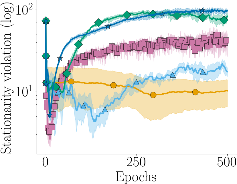 |
From Figure 1, we can see that VRLM (both variants) outperform all competing methods in terms of training loss and testing accuracy, while VRLM-STORM can additionally find sparser solutions. For this problem, DM-HSGD is not competitive when . All methods appear to struggle with reducing (4.2) for both datasets, but we remark that this does not appear to affect each method’s ability to minimize the training loss and obtain reasonable testing accuracy.
4.2 Fair Classification
We also test our method on the Fair Classification problem Mohri2019 using the CIFAR-10 krizhevsky09 dataset. Each agent maintains a local dataset, , where is the -th image on the -th agent and is the corresponding label. The agents’ local objective functions are given by
| (4.3) |
where denotes the -th component of , is the cross-entropy loss function which computes the average loss over each class, is a neural network governed by the parameter , is a parameter to tune, and is the standard probability simplex. We choose to be the All-CNN network springenberg15 and let .
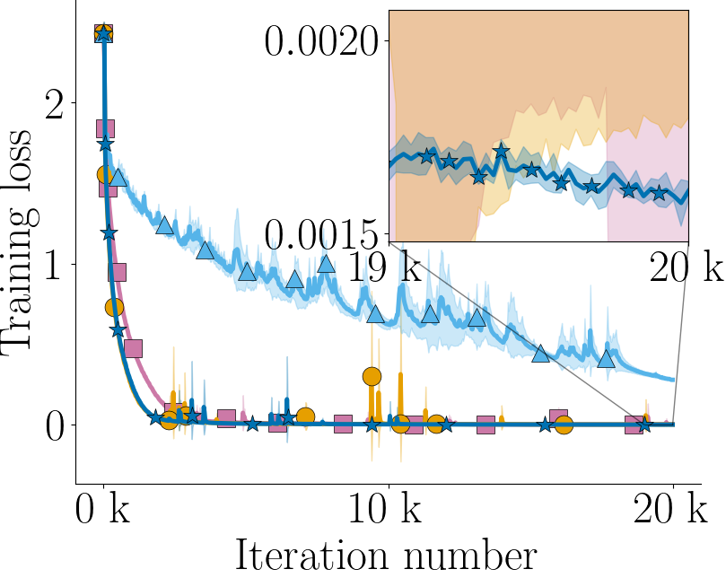
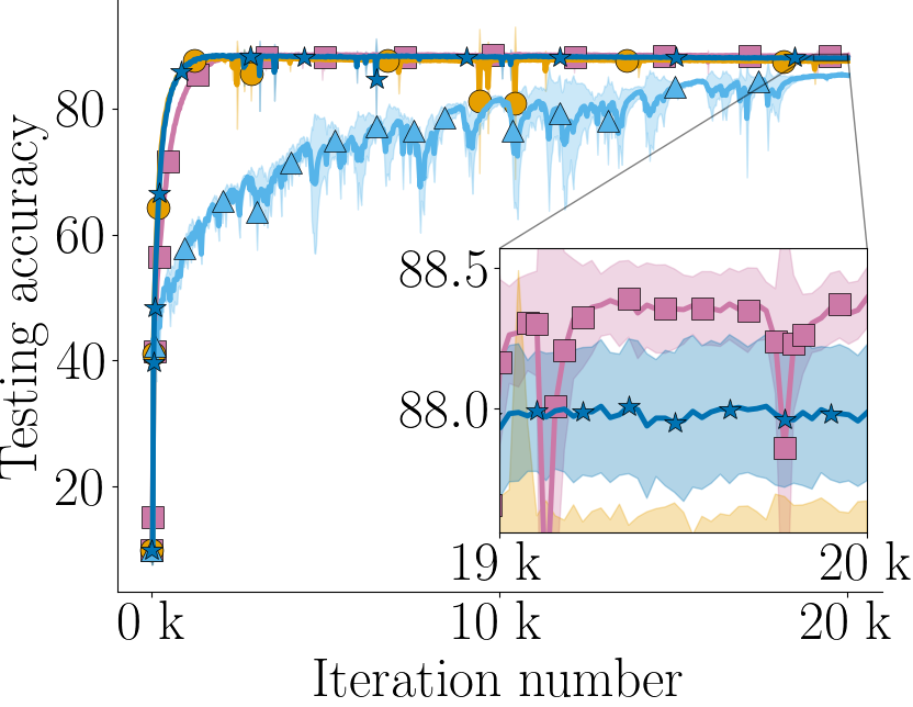
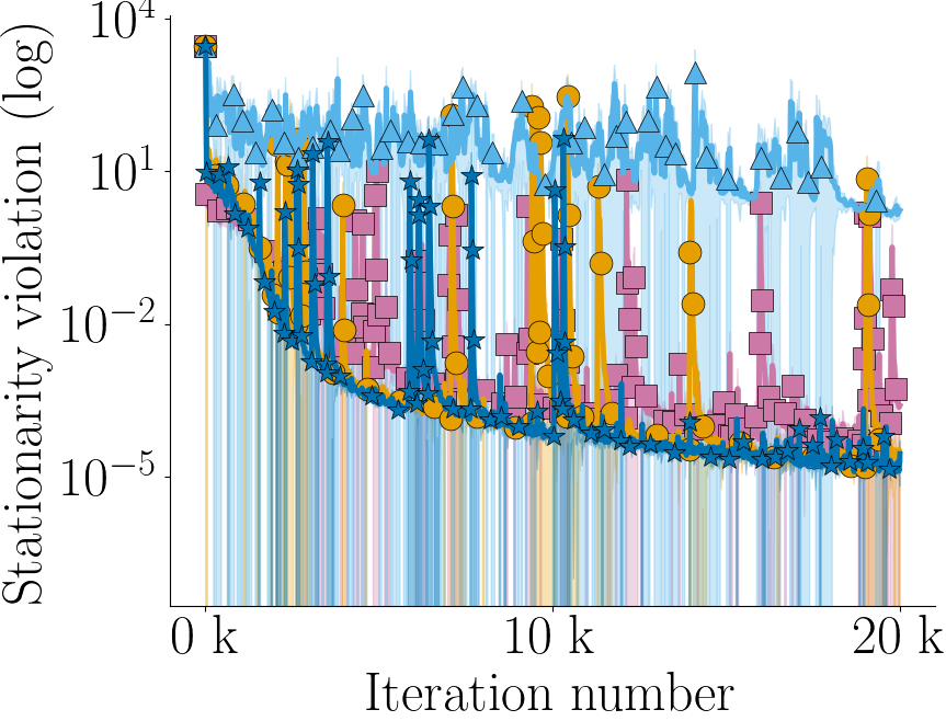
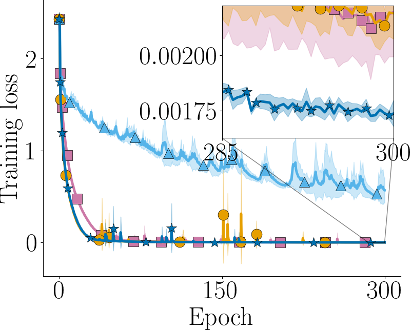
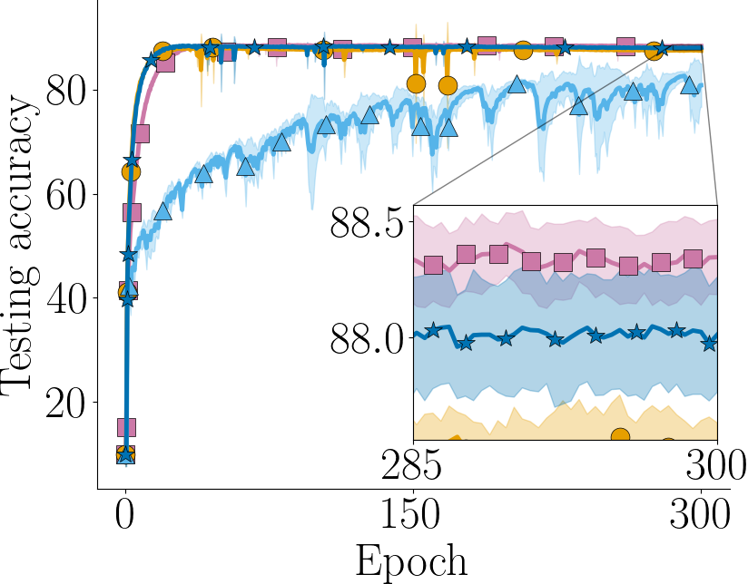
The dataset is split uniformly at random among the agents, hence each agent receives local data points. We let the mini-batch size for all methods be 100 and tune and . For DM-HSGD, we tune and set the initial batch-size to 3000. For GT-SRVR, we tune and the large mini-batch size from . For VRLM-STORM, we tune and let and . We found VRLM-SPIDER noncompetitive on this instance, and the results are omitted. We run all methods to iterations and compare the training loss value (as if performing centralized training; note this is not the objective value), testing accuracy, and stationarity violation, where the stationarity violation is computed as
| (4.4) |
where for . We use (4.4) instead of (4.2) due to the memory constraint of our computing environment which prohibits us from putting all the data on one machine. Again, we run each experiment with 5 different initial seeds and report the average results across both iterations and epochs.
 |
 |
 |
 |
 |
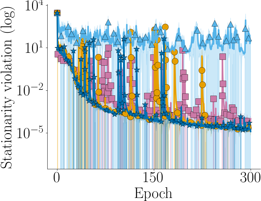 |
From Figure 2, we can see that DM-HSGD and our proposed method perform similarly in terms of stationarity violation. However, our method can achieve higher testing accuracy and lower training loss. DPOSG yields high testing accuracy, but its convergence for the double-regularized problem (2.2) has not been studied. The GT-SRVR method is not competitive on this problem, which could be due to the lack of theoretical guarantees for the double-regularized problem (2.2), or due to the periodic large-batch stochastic gradient computation. Overall, we find our proposed method to be competitive against other state-of-the-art methods, while providing improved theoretical guarantees.
5 Conclusions
In this work, we have presented the Variance Reduced Lagrangian Multiplier (VRLM) based method for solving the decentralized, double-regularized, stochastic nonconvex strongly-concave minimax problem. We analyzed VRLM with both big-batch and small-batch variance-reduction techniques. Under mild assumptions, both versions are able to achieve the best-known complexity results that are achieved by existing methods for solving special cases of the problem we consider. Finally, we demonstrated the effectiveness of our proposed methods in a real decentralized computing environment on two benchmark machine learning problems.
Appendix A Proof of Lemma 3.1
By the definition of in (3.3) and (3.6), we have
| (A.1) | ||||
where the first inequality follows from the triangle inequality and the nonexpansiveness of , the second inequality uses the update of and the triangle inequality, and the last inequality holds by for all . Squaring both sides of (A), using Young’s inequality, and summing over with the definition of in (3.4) yields
| (A.2) |
where we have used to have . By multiplying to (A.2), adding , and using , we obtain
| (A.3) |
This completes the proof of (3.14). Again, by the definition of in (3.3), in conjunction with (3.6) and Young’s inequality, we have
| (A.4) |
where we have used (2.7), by Assumption 3.2, and (3.11). This completes the proof.
Appendix B Proof of Lemma 3.2
To prove Lemma 3.2, we first state a few supporting lemmas. The following lemma can be proved in the same way as the proof of (mancino2022proximal, , Lemma C.3).
Lemma B.1
For all and for all ,
| (B.1) |
Lemma B.2
For all and arbitrary constants , the following inequality holds
| (B.2) |
Proof
By the -smoothness of defined in (3.1), it holds that
| (B.3) | ||||
where the second inequality uses the convexity of to have and (B.1). By the definition of in (3.6) and the definition of in (3.3), we have
| (B.4) |
By the -smoothness of and the Peter-Paul inequality, we further have
| (B.5) | ||||
where the last inequality uses (3.10b). Additionally, by the Peter-Paul inequality,
| (B.6) |
where the last inequality uses (3.10b). Plugging (B) and (B) into (B.4) results in
| (B.7) |
Lemma B.3
For all , it holds that
| (B.8) |
where is an arbitrary constant.
Proof
Notice
Then the desired result follows from the Peter-Paul inequality.
Appendix C Proofs of Lemmas in Section 3.3
Proof (Of Lemma 3.4)
By Young’s inequality, it holds that
where the second inequality follows from Jensen’s inequality and . Taking the expectation yields (3.19).
Proof (Of Lemma 3.5)
By the update defined in (2.8), it holds for all that
| (C.1) |
and hence for some and any , it holds that
| (C.2) |
By the convexity of , we further have
| (C.3) |
Summing (C.3) over and taking for all gives
| (C.4) |
Now by the definition of from (3.5) and the update for from (2.6), it holds that
| (C.5) |
By Assumption 3.3, is -smooth for all and hence
| (C.6) |
where we have used the definition of from (3.4). Next, we compute
| (C.7) | ||||
where the inequality uses Assumption 3.3 and is defined in (3.3) for all By
we obtain from (3.13) that
| (C.8) |
Applying (C.8) to (C) and rearranging results in
| (C.9) |
Adding times of (C.9) to (C) results in
| (C.10) |
Applying (C.10) to (C.4), using the definition of from (3.21), and rearranging terms results in
| (C.11) | ||||
By the Peter-Paul inequality, we have that for any ,
| (C.12) | |||
| (C.13) | |||
| (C.14) |
where we have used Assumption 3.3 in (C.13) and Assumption 3.2 in (C.14). Applying (C.12)-(C.14) to (C.11) results in
| (C.15) |
By , it holds that and hence
| (C.16) |
Applying completes the proof.
Proof (Of Lemma 3.6)
By the definition of in (3.3), it holds that
| (C.17) |
Defining , we have for all ,
| (C.18) |
where denotes the -th row of . Hence,
| (C.19) |
By the non-expansiveness of the proximal operator,
| (C.20) |
Utilizing the -update (2.6) in (C) and the Peter-Paul inequality we obtain
| (C.21) |
where is an arbitrary constant. By the -smoothness and -strong convexity of , it holds for all that
| (C.22) |
where the second to last inequality uses the strong concavity of and the last uses to have . Hence, by the Peter-Paul inequality and utilizing (C) within (C.21), we have
| (C.23) | ||||
where is an arbitrary constant. Setting and in (C) and utilizing , it holds that
| (C.24) | |||
| (C.25) | |||
| (C.26) |
Applying the bounds in (C.24)-(C.26) to (C) and utilizing completes the proof.
Appendix D Proofs of Lemmas and Corollary in Section 3.4
Proof (Of Lemma 3.7)
We first prove (3.24), for which we break the proof into two cases. For the first case, we assume , i.e., is divisible by . Then for all , we have by the definition of that
| (D.1) |
where the second equality uses the law of total expectation and the inequality uses Assumption 3.3(ii) and . Next, we assume and compute
| (D.2) |
where the inequality comes from Eqn. (A.4) in fang18spider . Recursively utilizing (D.2) for and using (D.1) with yields
| (D.3) |
For (3.23), we utilize the technique from Lemma C.7 in mancino2022proximal to have
| (D.4) |
By , we use Young’s inequality to have
| (D.5) |
where the last inequality further uses Assumption 3.3. Take the expectation of (D) and utilize (3.24) to have
| (D.6) |
Applying (D.6) to the expectation of (D.4) and further using the non-negativity of the 2-norm completes the proof.
Proof (Of Lemma 3.8)
Proof (Of Corollary 1)
By the choice of initialization and the definition of from Theorem 3.1, we have
Additionally by (3.30) and , the stepsizes in (3.30) are and . Thus we have from (3.45) that
and similarly
Thus for the finite-sum setting, since , we can produce an -stationary point as defined in Definition 3.1 by iterations, with
| (D.9) |
For the general case, , and an -stationary point can be produced with and in the same order as that in (D.9). For both general case and finite-sum case, we set . Noticing the total number of communication is and the total number of sample gradients , we complete the proof.
Appendix E Proofs of Lemmas and Corollary in Section 3.5
Proof (Of Lemma 3.9)
For (3.51), we use (D.4). When VR-tag == STORM in Algorithm 1, it holds
| (E.1) |
Using Young’s inequality and taking the expectation with respect to the samples and then the full expectation yields
| (E.2) |
where is defined as the -th row of for all and we have additionally used Assumption 3.3(ii). Taking the full expectation of (D.4) and applying (E.1) with (E.2) summed over yields (3.51). The proof of (3.52) follows from the same arguments of the proof of (mancino2022proximal, , Lemma C.9).
Proof (Of Lemma 3.10)
We first take the expectation of (3.16), apply (3.19), and plug in the values of and specified in (3.53) to have
| (E.3) |
where the coefficient of is obtained by using and to have
Next, for any , we add to both sides of (E.3) and upper bound the right-hand side using Lemmas 3.3, 3.6, and 3.9 to obtain
| (E.4) | ||||
We apply and (3.20) to (E) to have
| (E.5) | ||||
Next, we utilize (3.7) to bound . Then we subtract from both sides of (E) with
| (E.6) |
to have
| (E.7) |
Set
| (E.8a) | |||
| (E.8b) | |||
| (E.8c) | |||
| (E.8d) | |||
By the definition of and , we can easily have and thus . Then by the choice of , , and , it follows that
| (E.9) |
where the last inequality uses Hence by the choice of , , , and (E.9), we additionally have
| (E.10) |
Moreover, applying , , (E.9), and (E.10) to (E.8c) yields Thus by the upper bounds of and together with yields
| (E.11) |
Hence, from the definition of in (E.6) and (E.10), (E.11), it follows
| (E.12) |
where the last inequality follows from the definition of In addition, by , , (E.10), and (E.11), we have
By the above equation and the choice of , we have
| (E.13) |
On the other hand, from (E) and the definition of , it follows
| (E.14) |
Additionally, by the definition of and , (3.39) holds, and thus
| (E.15) |
Also, by the choice of and and , it holds that
| (E.16) |
Furthermore, from and the formula of , it holds that
| (E.17) |
Applying (E.13)-(E) to (E.7), summing over to , and finally using and the upper bounds on completes the proof.
Proof (Of Corollary 2)
By the choice of in (3.59) and the upper bound of , it holds that . Thus a straight-forward comparison of the two fractions in (3.54a) and (3.54b) yields
References
- [1] Y. Arjevani, Y. Carmon, J. C. Duchi, D. J. Foster, N. Srebro, and B. Woodworth. Lower bounds for non-convex stochastic optimization. Mathematical Programming, 199(1-2):165–214, 2023.
- [2] L. Chen, H. Ye, and L. Luo. A simple and efficient stochastic algorithm for decentralized nonconvex-strongly-concave minimax optimization. arXiv preprint arXiv:2212.02387, 2022.
- [3] Z. Chen, S. Ma, and Y. Zhou. Accelerated proximal alternating gradient-descent-ascent for nonconvex minimax machine learning. arXiv preprint arXiv:2112.11663, 2021.
- [4] A. Cutkosky and F. Orabona. Momentum-based variance reduction in non-convex sgd. Advances in neural information processing systems, 32, 2019.
- [5] J. M. Danskin. The theory of max-min, with applications. Siam Journal on Applied Mathematics, 14:641–664, 1966.
- [6] A. Defazio, F. Bach, and S. Lacoste-Julien. SAGA: A fast incremental gradient method with support for non-strongly convex composite objectives. Advances in neural information processing systems, 27, 2014.
- [7] D. Drusvyatskiy and A. S. Lewis. Error bounds, quadratic growth, and linear convergence of proximal methods. Mathematics of Operations Research, 43(3):919–948, 2018.
- [8] C. Fang, C. J. Li, Z. Lin, and T. Zhang. Spider: Near-optimal non-convex optimization via stochastic path integrated differential estimator. In Proceedings of the 32nd International Conference on Neural Information Processing Systems, page 687–697, Red Hook, NY, USA, 2018. Curran Associates Inc.
- [9] P. Foret, A. Kleiner, H. Mobahi, and B. Neyshabur. Sharpness-aware minimization for efficiently improving generalization. In International Conference on Learning Representations, 2021.
- [10] H. Gao. Decentralized stochastic gradient descent ascent for finite-sum minimax problems. arXiv preprint arXiv:2212.02724, 2022.
- [11] I. Goodfellow, J. Pouget-Abadie, M. Mirza, B. Xu, D. Warde-Farley, S. Ozair, A. Courville, and Y. Bengio. Generative adversarial nets. In Z. Ghahramani, M. Welling, C. Cortes, N. Lawrence, and K. Weinberger, editors, Advances in Neural Information Processing Systems, volume 27. Curran Associates, Inc., 2014.
- [12] F. Huang, S. Gao, J. Pei, and H. Huang. Accelerated zeroth-order and first-order momentum methods from mini to minimax optimization. Journal of Machine Learning Research, 23(36):1–70, 2022.
- [13] C. Jin, P. Netrapalli, and M. Jordan. What is local optimality in nonconvex-nonconcave minimax optimization? In International Conference on Machine Learning, pages 4880–4889. PMLR, 2020.
- [14] N. S. Keskar, D. Mudigere, J. Nocedal, M. Smelyanskiy, and P. T. P. Tang. On large-batch training for deep learning: Generalization gap and sharp minima. In 5th International Conference on Learning Representations, ICLR 2017, Toulon, France, April 24-26, 2017, Conference Track Proceedings. OpenReview.net, 2017.
- [15] A. Koloskova, T. Lin, and S. U. Stich. An improved analysis of gradient tracking for decentralized machine learning. In A. Beygelzimer, Y. Dauphin, P. Liang, and J. W. Vaughan, editors, Advances in Neural Information Processing Systems, 2021.
- [16] A. Krizhevsky. Learning multiple layers of features from tiny images. Technical report, 2009.
- [17] Y. Lecun, L. Bottou, Y. Bengio, and P. Haffner. Gradient-based learning applied to document recognition. Proceedings of the IEEE, 86(11):2278–2324, 1998.
- [18] J. Li, L. Zhu, and A. M.-C. So. Global convergence rate analysis of nonsmooth nonconvex-nonconcave minimax optimization. arXiv preprint arXiv:2209.10825v2, 2023.
- [19] X. Lian, C. Zhang, H. Zhang, C.-J. Hsieh, W. Zhang, and J. Liu. Can decentralized algorithms outperform centralized algorithms? a case study for decentralized parallel stochastic gradient descent. In I. Guyon, U. V. Luxburg, S. Bengio, H. Wallach, R. Fergus, S. Vishwanathan, and R. Garnett, editors, Advances in Neural Information Processing Systems, volume 30, pages 5330–5340. Curran Associates, Inc., 2017.
- [20] T. Lin, C. Jin, and M. Jordan. On gradient descent ascent for nonconvex-concave minimax problems. In International Conference on Machine Learning, pages 6083–6093. PMLR, 2020.
- [21] T. Lin, C. Jin, and M. I. Jordan. Near-optimal algorithms for minimax optimization. In Conference on Learning Theory, pages 2738–2779. PMLR, 2020.
- [22] M. Liu, W. Zhang, Y. Mroueh, X. Cui, J. Ross, T. Yang, and P. Das. A decentralized parallel algorithm for training generative adversarial nets. In H. Larochelle, M. Ranzato, R. Hadsell, M. Balcan, and H. Lin, editors, Advances in Neural Information Processing Systems, volume 33, pages 11056–11070. Curran Associates, Inc., 2020.
- [23] Z. Liu, X. Zhang, S. Lu, and J. Liu. Precision: Decentralized constrained min-max learning with low communication and sample complexities. arXiv preprint arXiv:2303.02532, 2023.
- [24] P. D. Lorenzo and G. Scutari. Next: In-network nonconvex optimization. IEEE Transactions on Signal and Information Processing over Networks, 2(2):120–136, 2016.
- [25] S. Lu, X. Zhang, H. Sun, and M. Hong. Gnsd: a gradient-tracking based nonconvex stochastic algorithm for decentralized optimization. In 2019 IEEE Data Science Workshop (DSW), pages 315–321, 2019.
- [26] Y. Lu and C. De Sa. Optimal complexity in decentralized training. In International Conference on Machine Learning, pages 7111–7123. PMLR, 2021.
- [27] L. Luo, H. Ye, Z. Huang, and T. Zhang. Stochastic recursive gradient descent ascent for stochastic nonconvex-strongly-concave minimax problems. In H. Larochelle, M. Ranzato, R. Hadsell, M. Balcan, and H. Lin, editors, Advances in Neural Information Processing Systems, volume 33, pages 20566–20577. Curran Associates, Inc., 2020.
- [28] G. Mancino-Ball, S. Miao, Y. Xu, and J. Chen. Proximal stochastic recursive momentum methods for nonconvex composite decentralized optimization. arXiv preprint arXiv:2211.11954, 2022.
- [29] G. Mancino-Ball, Y. Xu, and J. Chen. A decentralized primal-dual framework for non-convex smooth consensus optimization. IEEE Transactions on Signal Processing, 71:525–538, 2023.
- [30] M. Mohri, G. Sivek, and A. T. Suresh. Agnostic federated learning. In K. Chaudhuri and R. Salakhutdinov, editors, Proceedings of the 36th International Conference on Machine Learning, volume 97 of Proceedings of Machine Learning Research, pages 4615–4625. PMLR, 09–15 Jun 2019.
- [31] H. Namkoong and J. C. Duchi. Stochastic gradient methods for distributionally robust optimization with f-divergences. In D. Lee, M. Sugiyama, U. Luxburg, I. Guyon, and R. Garnett, editors, Advances in Neural Information Processing Systems, volume 29. Curran Associates, Inc., 2016.
- [32] A. Nedic, A. Olshevsky, and W. Shi. Achieving geometric convergence for distributed optimization over time-varying graphs. SIAM Journal on Optimization, 27:2597 – 2633, 2017.
- [33] Y. Nesterov. Gradient methods for minimizing composite functions. Mathematical Programming, 140(1):125–161, 2013.
- [34] L. M. Nguyen, J. Liu, K. Scheinberg, and M. Takáč. SARAH: A novel method for machine learning problems using stochastic recursive gradient. In International conference on machine learning, pages 2613–2621. PMLR, 2017.
- [35] M. Nouiehed, M. Sanjabi, T. Huang, J. D. Lee, and M. Razaviyayn. Solving a class of non-convex min-max games using iterative first order methods. In Advances in Neural Information Processing Systems, volume 32. Curran Associates, Inc., 2019.
- [36] D. M. Ostrovskii, A. Lowy, and M. Razaviyayn. Efficient search of first-order nash equilibria in nonconvex-concave smooth min-max problems. SIAM Journal on Optimization, 31(4):2508–2538, 2021.
- [37] G. Scutari and Y. Sun. Distributed nonconvex constrained optimization over time-varying digraphs. Mathematical Programming, 176:497–544, 2019.
- [38] W. Shi, Q. Ling, G. Wu, and W. Yin. Extra: An exact first-order algorithm for decentralized consensus optimization. SIAM Journal on Optimization, 25:944 – 966, 2015.
- [39] J. T. Springenberg, A. Dosovitskiy, T. Brox, and M. Riedmiller. Striving for simplicity: The all convolutional net. arXiv preprint arXiv:1412.6806, 2015.
- [40] H. Tang, X. Lian, M. Yan, C. Zhang, and J. Liu. : Decentralized training over decentralized data. In J. Dy and A. Krause, editors, Proceedings of the 35th International Conference on Machine Learning, volume 80 of Proceedings of Machine Learning Research, pages 4848–4856, Stockholmsmässan, Stockholm Sweden, 10–15 Jul 2018. PMLR.
- [41] K. K. Thekumparampil, P. Jain, P. Netrapalli, and S. Oh. Efficient algorithms for smooth minimax optimization. Advances in Neural Information Processing Systems, 32, 2019.
- [42] I. Tsaknakis, M. Hong, and S. Liu. Decentralized min-max optimization: Formulations, algorithms and applications in network poisoning attack. In ICASSP 2020 - 2020 IEEE International Conference on Acoustics, Speech and Signal Processing (ICASSP), pages 5755–5759, 2020.
- [43] J. Verbraeken, M. Wolting, J. Katzy, J. Kloppenburg, T. Verbelen, and J. S. Rellermeyer. A survey on distributed machine learning. ACM Comput. Surv., 53(2), mar 2020.
- [44] W. Xian, F. Huang, Y. Zhang, and H. Huang. A faster decentralized algorithm for nonconvex minimax problems. In M. Ranzato, A. Beygelzimer, Y. Dauphin, P. Liang, and J. W. Vaughan, editors, Advances in Neural Information Processing Systems, volume 34, pages 25865–25877. Curran Associates, Inc., 2021.
- [45] H. Xiao, K. Rasul, and R. Vollgraf. Fashion-mnist: a novel image dataset for benchmarking machine learning algorithms. arXiv preprint arXiv:1708.07747, 2017.
- [46] R. Xin, S. Das, U. A. Khan, and S. Kar. A stochastic proximal gradient framework for decentralized non-convex composite optimization: Topology-independent sample complexity and communication efficiency. arXiv preprint, arXiv:2110.01594, 2021.
- [47] R. Xin, U. Khan, and S. Kar. A hybrid variance-reduced method for decentralized stochastic non-convex optimization. In Proceedings of the 38th International Conference on Machine Learning, volume 139 of Proceedings of Machine Learning Research, pages 11459–11469. PMLR, 18–24 Jul 2021.
- [48] Y. Xu. Decentralized gradient descent maximization method for composite nonconvex strongly-concave minimax problems. arXiv preprint arXiv:2304.02441, 2023.
- [49] Y. Xu and Y. Xu. Momentum-based variance-reduced proximal stochastic gradient method for composite nonconvex stochastic optimization. Journal of Optimization Theory and Applications, 196(1):266–297, 2023.
- [50] Z. Xu, H. Zhang, Y. Xu, and G. Lan. A unified single-loop alternating gradient projection algorithm for nonconvex–concave and convex–nonconcave minimax problems. Mathematical Programming, pages 1–72, 2023.
- [51] J. Yang, A. Orvieto, A. Lucchi, and N. He. Faster single-loop algorithms for minimax optimization without strong concavity. In International Conference on Artificial Intelligence and Statistics, pages 5485–5517. PMLR, 2022.
- [52] J. Zhang and K. You. Decentralized stochastic gradient tracking for non-convex empirical risk minimization. arXiv preprint arXiv:1909.02712, 2020.
- [53] X. Zhang, N. Aybat, and M. Gurbuzbalaban. SAPD+: An accelerated stochastic method for nonconvex-concave minimax problems. In A. H. Oh, A. Agarwal, D. Belgrave, and K. Cho, editors, Advances in Neural Information Processing Systems, 2022.
- [54] X. Zhang, Z. Liu, J. Liu, Z. Zhu, and S. Lu. Taming communication and sample complexities in decentralized policy evaluation for cooperative multi-agent reinforcement learning. In M. Ranzato, A. Beygelzimer, Y. Dauphin, P. Liang, and J. W. Vaughan, editors, Advances in Neural Information Processing Systems, volume 34, pages 18825–18838. Curran Associates, Inc., 2021.
- [55] T. Zheng, L. Zhu, A. M.-C. So, J. Blanchet, and J. Li. Doubly smoothed gda: Global convergent algorithm for constrained nonconvex-nonconcave minimax optimization. arXiv preprint arXiv:2212.12978, 2022.